Tracing the Filamentary Structure of the Galaxy Distribution at $z\sim 0.8$

Abstract

We study filamentary structure in the galaxy distribution at $z\sim 0.8$ using data from the Deep Extragalactic Evolutionary Probe 2 (DEEP2) Redshift Survey and its evolution to $z\sim 0.1$ using data from the Sloan Digital Sky Survey (SDSS). We trace individual filaments for both surveys using the Smoothed Hessian Major Axis Filament Finder, an algorithm which employs the Hessian matrix of the galaxy density field to trace the filamentary structures in the distribution of galaxies. We extract 33 subsamples from the SDSS data with a geometry similar to that of DEEP2. We find that the filament length distribution has not significantly changed since $z\sim 0.8$, as predicted in a previous study using a $\Lambda$CDM cosmological N-body simulation. However, the filament width distribution, which is sensitive to the non-linear growth of structure, broadens and shifts to smaller widths for smoothing length scales of $5-10$ $h^{-1}$ Mpc from $z\sim 0.8$ to $z\sim 0.1$, in accord with N-body simulations.

1 Introduction

The observed large-scale distribution of galaxies shows dense linear features: filaments of galaxies which surround huge voids that appear largely empty, while rich clusters are found at their intersection (Davis et al., 1982; de Lapparent, Geller, & Huchra, 1986; Bond & Myers, 1996; Gott et al., 2005). These structures are widely believed to have evolved through gravitational instability from small density fluctuations in the early universe. The evolution of large scale structure with cosmic time can probe the complex physics that governs the creation of galaxies in their host dark matter potential wells. A number of studies (e.g. Cohen et al., 1996; Connolly et al., 1996; Giavalisco et al., 1998; Brown et al., 2003; Phleps & Meisenheimer, 2003; Coil et al., 2004b; Ouchi et al., 2004; Le Fèvre et al., 2005; Meneux et al., 2006) have focused on the redshift dependence of the galaxy two point correlation function as a critical test of both cosmological and galaxy evolution models. The comoving correlation length of galaxies is observed to be almost constant with redshift, which is interpreted as a consequence of the increasing bias of galaxies with redshift.

The two-point correlation function is a complete statistical measure of galaxy clustering only in the linear regime. Statistics of galaxy filaments, such as their lengths and widths, can be used as another useful tool to measure the large scale structure and test both cosmology and galaxy formation models. Filaments, with a typical length of $50-70$ $h^{-1}$ Mpc (Bharadwaj, Bhavsar & Sheth, 2004), have been seen in every wide-field redshift survey, from the Great Wall of the CFA2 (de Lapparent, Geller, & Huchra, 1986; Geller & Huchra, 1989) to the very long filaments found (Gott et al., 2005) in the Sloan Digital Sky Survey (SDSS) (York et al., 2000). Features qualitatively similar to the observed filamentary structures are also seen in numerical cosmological simulations. Various techniques have been proposed to identify and characterize filaments in observational and simulated samples (e.g. Moody, Turner & Gott, 1983; Eriksen et al., 2004; Stoica et al., 2005; Lacoste et al., 2005; Novikov, Colombi & Doré, 2006; Aragón-Calvo et al., 2007; Sousbie et al., 2008a, b; Soubie, Colombi & Pichon, 2009; Forero-Romero et al., 2009). Bond, Strauss, & Cen (2009, 2010, hereafter Paper I and II, repectively) use the eigenvectors of the Hessian matrix of the smoothed galaxy density field to identify and quantify filamentary structures. The filament length and width distributions of the observed local galaxy distribution from SDSS are consistent with those from N-body simulations at $z\sim 0$ adopting a standard cosmology. The time evolution of the filament network was studied in Paper II using cosmological N-body simulations; they found that the backbone of the filamentary structure is in place at $z=3$. These simulations show that non-linear growth of structure has little impact on the length of filamentary structures, but a great deal on the width. The dark matter filament width distribution evolves from $z\sim 3$ to $z\sim 0$, broadening and peaking at smaller widths as the universe expands.

Although many recent papers have studied the filamentary structures of local galaxy surveys (Stoica et al., 2007; Sousbie et al., 2008a, b; Gay et al., 2009), no study has been done on the evolution of filaments in redshift survey data. This is mainly due to the small volumes and the resulting severe cosmic variance of existing high redshift surveys. However, thanks to the successful completion of the Deep Extragalactic Evolutionary Probe 2 (DEEP2) Galaxy Redshift Survey (Davis et al., 2003), we can study the galaxy distribution at $z\sim 1$ over a large comoving volume ($5\times 10^{6}$ $h^{-3}\rm Mpc^{3}$) over four widely separated fields.

In this study, we present measurements of filament statistics both for the galaxy distribution at $z\sim 0.8$ using the DEEP2 Galaxy Redshift Survey (Davis et al., 2003), which is an R-band-selected survey with a sampling density comparable to local surveys, and for the local galaxy distribution from the SDSS. We identify filaments in the galaxy distribution in DEEP2 using the Hessian matrix method of Paper I and II, and draw subsamples from the SDSS redshift survey with the DEEP2 geometry and sampling, to make a direct comparison between the two.

This paper is organized as follows: § 2 summarizes the methods we use to find filamentary structures and measure their properties, referring the reader to Paper I and Paper II for more details. In § 3, we provide details of the data samples used here. § 4 presents our results and § 5 discusses their meaning and implications. We assume a flat concordance $\Lambda$CDM cosmology with $\Omega_{m}=0.3$, $\Omega_{\Lambda}=1-\Omega_{m}=0.7$ and $H_{0}=100$ $h$ km s^-1 Mpc^-1 throughout this paper.

2 Methods

In this paper, we use the Smoothed Hessian Major Axis Filament Finder (SHMAFF), an algorithm that uses the eigenvectors of the Hessian matrix of the smoothed galaxy distribution to identify filamentary structures of galaxy data. The detailed methodology of SHMAFF and its applications are described in Papers I and II; Paper I quantifies the prominence and shapes of structures in the galaxy distribution using the Hessian matrix, while Paper II describes a method to find individual filaments, and compares their properties in cosmological N-body simulations to those in the SDSS galaxy distribution. We summarize the basics here. Since the geometry of the DEEP2 fields allows us to study filamentary structures best in two dimensions, we use a two-dimensional version of SHMAFF in this study.

2.1 Smoothed density field and its Hessian

To trace individual filaments in the galaxy distribution, we generate the density field and its second derivatives; filaments will be defined as regions with one eigenvalue of the Hessian matrix much larger than the other two. The density field is smoothed with a Gaussian kernel with smoothing length $l$,

$$\tilde{\rho}({\bf x})=\int f({\bf x}-{\bf x^{\prime}})\rho({\bf x^{\prime}}){\rm d}^{2}{\bf x^{\prime}},$$ (1)

where $\rho(x)$ is the unsmoothed density field, and $f(x)$ is the smoothing kernel. In this study we use Gaussian smoothing,

$$f({\bf x})=\frac{1}{\sqrt{2\pi l^{2}}}e^{\frac{-|{\bf x}|^{2}}{2l^{2}}},$$ (2)

where $l$ is the smoothing length and the smoothing is performed over a two-dimensional box. The unsmoothed density field is given as a sum of delta functions at the positions of the galaxies and the smoothed Hessian (the matrix of second partial derivatives) is given by

$$\tilde{H}_{{\rm ij}}({\bf x})=\int f({\bf x}-{\bf x^{\prime}})\frac{{\rm\partial}^{2}\rho({\bf x^{\prime}})}{{\rm\partial}x_{\rm i}^{\prime}{\rm\partial}x_{\rm j}^{\prime}}{\rm d}^{2}{\bf x^{\prime}}=-\int\frac{{\rm\partial}^{2}f({\bf x}-{\bf x^{\prime}})}{{\rm\partial}x_{\rm i}^{\prime}{\rm\partial}x_{\rm j}^{\prime}}\rho({\bf{\bf x^{\prime}}}){\rm d}^{2}{\bf x^{\prime}}.$$ (3)

Since the filamentary structures can appear on a variety of scales, it is important to smooth on a series of length scales $l$ when searching for filaments.

The Hessian matrix describes the local curvature of the density field, that is, the major axis is aligned along the direction of lowest concavity. We compute the eigenvalues, $\lambda_{i}$ of the Hessian matrix defined such that $\lambda_{1}<\lambda_{2}$, and eigenvectors, $\bf A_{i}$, which give the orientation of the structure at a given grid cell. The direction of lowest concavity is expected to be along the filament itself. We thus simply need to find the major axis of the Hessian ellipsoid in order to find the direction of a filament at a given point in space.

2.2 Filament-Finding Parameters

We trace filaments over those grid cells that satisfy the criteria $\lambda_{1}<0$, $\rho>\bar{\rho}$, where $\bar{\rho}$ is the mean density of the smoothed density field. We choose a starting point at the local maximum density, and trace out the filament both parallel and antiparallel to the $\bf A_{2}$ axis until its local curvature exceeds a given threshold. Along a filament, if the angular rate of change of the axis of structure exceeds a value $C$, filament tracing is stopped and the point will be marked as a filament end. The stopping condition at pixel $m$ is given by

$$|{\bf A_{2,m}}\times{\bf A_{2,m-1}}|>{\rm sin}(C\Delta),$$ (4)

where $\Delta$ is the distance between pixels.

As each filament is found, the pixels associated with it are removed from further consideration as filament starting points. In particular, we introduce another input parameter $K$ and define a removal width $W_{i}$ at grid cell $i$ as

$$W_{i}=K\sqrt{\frac{-\rho_{i}}{\lambda_{1,i}}}.$$ (5)

All pixels within a removal width $W_{i}$ of the most recently chosen filament element are excluded in the next iteration of the filament finding procedure, which prevents filaments from being multiply counted. Here, a filament element is defined to be a segment of the filament with length equal to the distance between pixels.

This process depends on three input parameters: the smoothing length $l$ ($h^{-1}$ Mpc), the curvature criterion $C$ (${}^{\circ}l^{-1}$) and the width of filament removal $K$. For tracing filaments in the large-scale galaxy distribution, the best values of the input parameters suggested by Paper II are $C=30^{\circ}l^{-1}$ and $40^{\circ}l^{-1}$ on smoothing scales of $l=5$ and 10 $h^{-1}$ Mpc respectively, and $K=1$ for all smoothing scales. These parameters were determined in three dimension; we adopt these values here in two dimension.

2.3 Filament Measurement

The length of each filament is defined as the distance along the filament between its two ends, which are specified by Eq. 4 or where the density no longer exceeds the threshold. As discussed in Paper II, the filament finder would identify an isolated spherical over-dense region as a ”filament” of length of order the smoothing length. Thus in this paper, we exclude ”filaments” whose lengths are shorter than the smoothing length $l$.

The width of a filament element ($W$) is defined to be the root mean squared perpendicular offset of galaxies within a smoothing length $l$:

$$W=\sqrt{\frac{\Sigma_{i=1}^{N}|{\rm\bf R}_{i}|^{2}}{N}},$$ (6)

where the sum is over the $N$ galaxies within a smoothing length of the filament element. Here, ${\rm\bf R}_{i}$ is the perpendicular offset of nearby points from the filament axis, and is defined as

$${\rm\bf R}_{i}={\rm\bf\hat{A}}_{j}\times({\rm\bf\hat{A}}_{i}\times({\rm\bf x}_{j}-{\rm\bf x}_{i})),$$ (7)

where ${\rm\bf\hat{A}}_{j}$ is the unit vector along the axis of structure.

3 DATA

The main data analyzed in this paper come from the DEEP2 and SDSS surveys. We now describe these two surveys to understand the samples and their selection funtions.

3.1 DEEP2 Galaxy Redshift Survey

The high-redshift galaxy sample used in this paper is from the DEEP2 Galaxy Redshift Survey (Davis et al., 2003), which used the Deep Imaging and Multi-Object Spectrograph (DEIMOS) (Faber et al., 2003) on the 10 m Keck II telescope to obtain spectra of optically selected galaxies at $z\sim 1$. The selection was done from deep BRI photometry drawn from images taken with the CFHT12k camera on the Canada-France-Hawaii Telescope (CFHT) (Coil et al., 2004b). The DEEP2 spectra have a resolution of $R\sim 5000$, and rms redshift errors, which are determined from repeated observations, are $\sim 30$ $\rm km~{}s^{-1}$. The survey has measured high-confidence redshifts for $\sim 28,100$ galaxies in the redshift range of $0.7<z<1.5$ down to a limiting magnitude of $R_{AB}=24.1$. The survey spans a comoving volume of approximately $5\times 10^{6}$$h^{-3}\rm Mpc^{3}$, covering $\sim 3~{}\rm deg^{2}$ over four widely separated fields to limit the effect of cosmic variance. The DEEP2 observations, catalog construction, and data reduction are described in more detail in Davis et al. (2003); Coil et al. (2004a) and Davis, Gerke, & Newman (2004).

In fields 2, 3, and 4, the spectroscopic target galaxies are preselected using a color cut in $(B-R)$-$(R-I)$ space to ensure that most galaxies have redshifts greater than 0.75. With this color cut, $\sim 90$% of the targeted galaxies are at $z>0.75$, and only $\sim 3$% of the $z>0.75$ galaxies brighter than the magnitude limit are not selected (Davis et al., 2003). A fourth field, the extended Groth Strip (EGS), does not have this redshift preselection. We use the absolute B-band magnitudes ($M_{B}$) and restframe $U-B$ colors that are derived in Willmer et al. (2006); we apply no corrections for luminosity evolution. We create volume-limited samples as a function of $M_{B}$ in three fields covering $\sim 2.2~{}\rm deg^{2}$. The DEEP2 sample is not complete, and has a complicated angular mask. Details of sample definitions are discussed in Section  3.3.

3.2 SDSS

Figure 1: Aitoff projection in equatorial coordinates of the angular coverage of the SDSS Data Release 7 galaxy catalog (Abazajian et al., 2009). Marked with a black solid line is the region from which samples used in this paper were drawn ($8^{\rm h}\leq\alpha\leq 16^{\rm h}$ and $0^{\circ}\leq\delta\leq 60^{\circ}$).

We will compare the DEEP2 filamentary structures to those obtained from the SDSS at redshifts of $z\la 0.1$. The SDSS is an extensive photometric and spectroscopic survey, which has obtained photometry of a quarter of the sky and spectra of over 1.6 million objects. Imaging is obtained in the $u$, $g$, $r$, $i$, and $z$ bands (Fukugita et al., 1996; Smith et al., 2002; Ivezić et al., 2004) with a drift-scan camera with 30 2048$\times$2048 CCDs (Gunn et al., 1998) on a dedicated 2.5 m telescope (Gunn et al., 2006). Spectra are measured with two fiber-fed digital spectrographs on the same telescope. Galaxies are selected for spectroscopy based on a magnitude limit (Strauss et al., 2002). An overview of the data pipelines and data products is provided in the Early Data Release paper (Stoughton et al., 2002). The galaxy sample used in this paper are constructed from the SDSS Data Release 7 (Abazajian et al., 2009, hereafter DR7). As of DR7, the spectra of $\sim 930,000$ galaxies have been measured, covering 9380 $\rm deg^{2}$. Galaxy redshift errors are typically $\sim 30\rm km~{}s^{-1}$, which is similar to DEEP2.

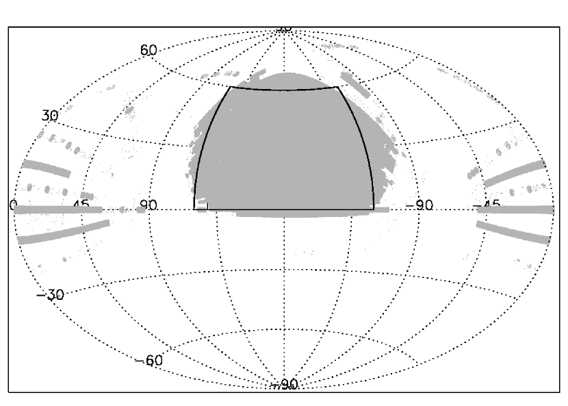
For this analysis, we make use of the New York University Value Added Galaxy Catalog (NYU-VAGC), which is a compilation of the galaxy catalog from the SDSS DR7, publicly available at http://sdss.physics.nyu.edu/vagc/. A detailed description can be found in Blanton et al. (2005). We construct volume-limited samples from the northern portion ($8^{\rm h}\leq\alpha\leq 16^{\rm h}$ and $0^{\circ}\leq\delta\leq 60^{\circ}$) of the survey as shown in Figure 1. We use $M_{{}^{0.1}r}$, the $r$-band absolute magnitude corrected to its $z=0.1$ value using the K-correction code of Blanton et al. (2003b) and the luminosity evolution model of Blanton et al. (2003c) to define volume-limited samples. We will define 33 subsamples from this SDSS sample volume shown in Figure 1 to match the geometry of the DEEP2 samples. Details of SDSS sample definitions and redshift range are discussed in Section 3.3.

3.3 Galaxy Sample Definitions

3.3.1 Absolute magnitude cut

Figure 2: (Top) Absolute B-band magnitude (in AB magnitudes, with $h=1$) vs. redshift of the DEEP2 galaxy catalog. The magnitude and redshift limits of the sample used here are shown in solid lines ($0.75\leq z\leq 0.92$ and $M_{B}\leq-19.47$). (Bottom) Absolute $M_{{}^{0.1}r}$ magnitude (with $h=1$) of SDSS DR7 galaxy catalog as a function of redshift. The magnitude and redshift limits of the main sample used here are shown as solid lines ($0.02\leq z\leq 0.10$ and $M_{{}^{0.1}r}$ $\leq-19.7$). The limits for the sparser sample used to study the effect of the direction of sample extraction (§3.3.2) are shown as dotted lines ($0.02\leq z\leq 0.15$ and $M_{{}^{0.1}r}$ $\leq-20.6$).

As explained in Paper II, sparse sampling of the galaxy density field can impact the filament detection rate. A small number of galaxies per smoothing volume can create false filament detections and cause real filaments to be missed. In order to make the most direct comparison of the DEEP2 and SDSS galaxy distribution, we need to make sure they have the same densities.

The mean galaxy comoving number density of galaxies with absolute magnitudes below an absolute magnitude $M_{cut}$ is:

$$n_{\Phi}=\int_{-\infty}^{M_{cut}}\Phi(M)dM,$$ (8)

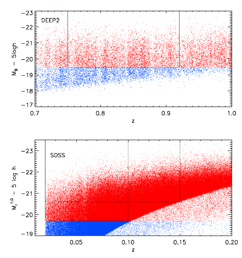
where $\Phi(M)$ is the luminosity function of the galaxy survey in question. We adopt Schechter (1976) fits from Blanton et al. (2003a) for the SDSS galaxy luminosity function and from Faber et al. (2007) for the DEEP2 luminosity function. We adjust the magnitude cut of each survey to define galaxy samples with matched number densities. We adopt the K-corrected rest-frame absolute magnitude cut $M_{B}=-19.47$ for DEEP2 and $M_{{}^{0.1}r}$ =$-19.7$ for SDSS with $h=1.0$, and for which the two samples have comparable mean number densities of $n_{\Phi}\sim 0.008$ $h^{3}\rm Mpc^{-3}$. These magnitude cuts are $\sim 1$ magnitude fainter than the characteristic magnitude $M^{*}$ of each survey. In Figure 2, we show the B-band absolute magnitude $M_{B}$ and redshift of each galaxy in the DEEP2 catalog and the regions from which our samples were drawn. The DEEP2 sample is volume-limited for blue galaxies, but not for red galaxies, due to the selection in the observed R band, which corresponds to the rest-frame UV (see Willmer et al. (2006) for more details on selection effects in the sample). Due to this selection effect and the lower sampling density beyond $z\sim 1$, we limit our filamentary study in this paper to $z<0.92$.

Figure 2 shows the absolute magnitude $M_{{}^{0.1}r}$ of each galaxy from the SDSS catalog and cuts in magnitude and redshift with solid lines. Our SDSS sample consists of 528343 main sample galaxies (Strauss et al., 2002) with $0.02<z<0.1$ and $M_{{}^{0.1}r}$ $<-19.7$.

The magnitude cuts were chosen to make the two samples have comparable number density $n_{\Phi}$ based on the luminosity functions. However, the DEEP2 redshift sample is roughly $35$% incomplete to its magnitude limit and redshift limit $0.75<z<0.92$, due to unobserved galaxies and redshift failures (Willmer et al., 2006) (this is in addition to the 3 % incompleteness of the color selection, as described in § 3.1). We thus apply the DEEP2 angular completeness window function to the SDSS sample to have the same number density ($n=0.005$ $h^{3}\rm Mpc^{-3}$) as the observed DEEP2 sample. We do this by selecting subsamples of SDSS with the same geometry as DEEP2, as we describe in Section 3.3.3 after we describe the DEEP2 geometry.

3.3.2 Subsample definition

Figure 3: Example of the subsample extraction from the DEEP2 $\it(top)$ and SDSS $\it(bottom)$ data. $\it Top:$ Redshift-space distribution of galaxies in Region 2 of DEEP2, shown as a function of redshift and comoving distance along the projected distance across the line of sight, assuming a $\Lambda$CDM cosmology. We extract one subsample from each region with dimensions of $320\times 40\times 14$ $\rm(h^{-1}Mpc)^{3}$ (in red). $\it Bottom:$ One slice with thickness of 14 $h^{-1}$ Mpc from SDSS: extracted subsamples are shown in red. We draw 33 such subsamples from the SDSS sample volume.

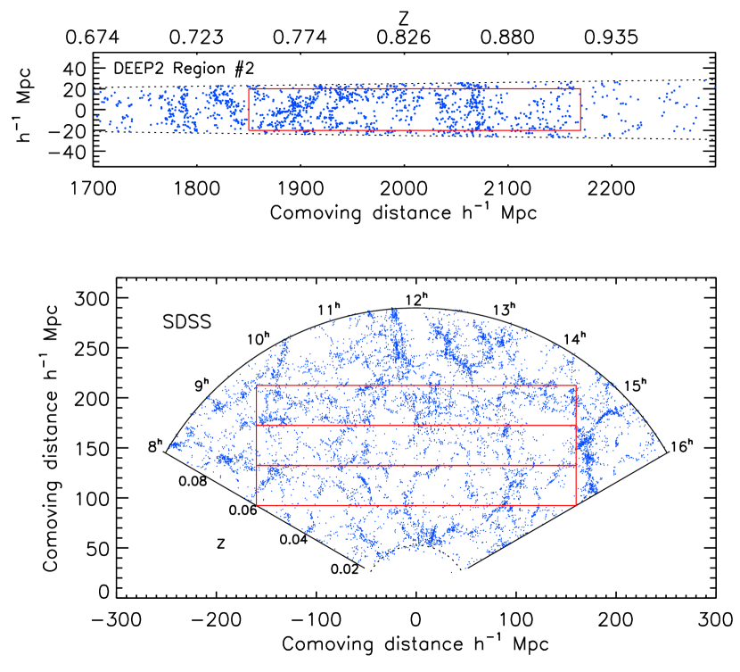
Each DEEP2 field is much longer in the redshift direction than on the sky; the $1-2\times 0.5$ deg² fields used for this work span $40-80\times 20$ $h^{-1}$ Mpc in transverse comoving extent, while the range $0.7<z<1.0$ corresponds to $560$ $h^{-1}$ Mpc comoving in the redshift direction. From this comoving volume, we select subsamples with dimension of $\rm L_{1}\times L_{2}\times L_{3}$ = $320\times 40\times 14$ $\rm(h^{-1}Mpc)^{3}$ =$179,200$ $h^{-3}\rm Mpc^{3}$, and define this as a standard box size. The comoving distance of the samples along the line of sight spans 1850 - 2170 $h^{-1}$ Mpc, which corresponds to $0.75<z<0.92$. We extract three subsamples, one from each region (see the example in the upper panel of Figure 3). We exclude the fourth field, the extended Groth Strip (EGS), which has a narrower width than other fields.

We can extract a larger number of subsamples with the standard box size out of the SDSS sample volume. We divide the volume into slices of thickness 14 $h^{-1}$ Mpc, and place as many rectangles into each slice as possible. Using this method, we obtain 33 subsamples in the redshift range of $0.02<z<0.10$. The bottom panel of Figure 3 shows an example of subsample extraction in an SDSS slice.

Figure 4: The width distributions (top) and the length distribution (bottom) of filaments of subsamples perpendicular (in blue) and parallel (in red) to the line of sight found with the smoothing length $l=5$ $\rm h^{-1}Mpc$, $C=30^{\circ}l^{-1}$, and $K=1$.

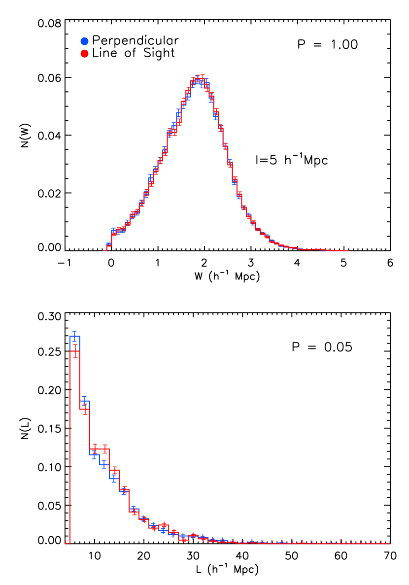
The long axis of the DEEP2 subsamples is along the redshift direction, while it is perpendicular to it in SDSS. One might be concerned that redshift distortions due to peculiar velocities along the line of sight would affect the filamentary statistics differently in the SDSS and DEEP2 subsamples. We were forced to do this, as the volume-limited SDSS sample has an extent in the radial direction less than the length of the standard box. We test the effect of the direction of sample extraction by comparing the filamentary properties from the subsamples extracted perpendicular to the line of sight to those extracted parallel to the line of sight. To do this, we build another sparser sample from the SDSS over the redshift range of $0.02<z<0.15$, with an absolute magnitude cut $M_{r^{0.1}}<-20.6$ (Figure 2). We extracted 135 subsamples perpendicular to the line of sight and 58 subsamples parallel to the line of sight. The filaments are found with the smoothing length $l=5$ $\rm h^{-1}Mpc$, $C=30^{\circ}l^{-1}$, and $K=1$. We derive the length and width distributions for each subsample and calculate the composite distributions and its error by calculating the mean and a standard deviation at each bin. As shown in Figure 4, we found that the filament width distributions are essentially indistinguishable between the perpendicular and parallel subsamples. This is confirmed by the Kolmogorov-Smirnov two-sample test (K-S test), which we applied to the two distributions. The length distributions of the two are essentially identical, differing by only 2 $\sigma$ by the K-S test. The effect of the direction of the subsample extraction on the filament finder and filamentary properties are negligible presumably because we smooth the density field with a smoothing length that is much larger than typical galaxy peculiar velocities.

Table 1: Summary of filamentary property

Smoothing length	5 $h^{-1}$ Mpc		10 $h^{-1}$ Mpc
data	DEEP2	SDSS	DEEP2	SDSS
Total number of filaments	97	958	24	245
mean $\#$ of filaments per subsample	$32.3\pm 4.7$	$29.0\pm 4.9$	$8.0\pm 1.7$	$7.42\pm 2.2$
mean total length of filaments ($h^{-1}$ Mpc)	$404.0\pm 29.5$	$376.1\pm 53.8$	$216.6\pm 20.0$	$186.5\pm 43.4$
width distribution peak $\mu$ ($h^{-1}$ Mpc)	$2.021\pm 0.009$	$1.924\pm 0.006$	$3.963\pm 0.023$	$3.802\pm 0.017$
width distribution $\sigma$ ($h^{-1}$ Mpc)	$0.508\pm 0.005$	$0.544\pm 0.004$	$0.580\pm 0.016$	$0.808\pm 0.011$

3.3.3 Survey completeness

We have to consider the survey completeness. The DEEP2 survey spectroscopically targets $\sim$60% of objects that pass the apparent magnitude and color cuts mentioned above. The redshift success is $73\%$ of those targeted galaxies (Willmer et al., 2006). Therefore, we have successful redshifts for $\sim 50$% of all galaxies in the surveyed fields with apparent magnitude of $R<24.1$. The sampling rate is a complex function of position across each field. In order to model this effect, we use the angular window function of the DEEP2 survey. The mask gives the completeness at each angular position; in unobserved regions such as around bright stars, the completeness is zero. We project the angular window function covering the three DEEP2 regions onto the geometry of each box to generate three-dimensional completeness maps. Then each SDSS subsample with the geometry of the DEEP2 standard box is diluted with a completeness map randomly selected among the three DEEP2 samples.

We have further complications because the sampling rate is non-uniform due to the necessities of slitmask design. Spectra of objects are not allowed to overlap on the CCD when observing with multi-object slit masks, therefore, objects that lie near each other in the direction on the sky that maps to the wavelength direction on the CCD cannot be observed simultaneously. This results in under-sampling in the highest density regions on the plane of the sky. In order to reduce the effect of this bias, adjoining slit masks are positioned approximately a half-mask width apart, giving each galaxy at least two chances to be on a mask (Coil et al., 2008). Despite this, the probability that a target with nearest neighbor $<10"$ away is selected for spectroscopy is diminished by $\sim 25\%$. Many DEEP2 related papers (Coil et al., 2004a; Conroy et al., 2005) model this effect by applying the actual DEEP2 mask-making algorithm to the mock galaxy catalogs, which throws out some galaxies located close to other galaxies in the sky. This effect on the filamentary properties is negligible, as it is more relevant on small scales $\la 2$ $\rm h^{-1}Mpc$ (Coil et al., 2006). In particular, Coil et al. (2008) have studied the bias in the two-point correlation function due to the slitmask effect; they found it was 3.5 % at 1 $h^{-1}$ Mpc, 1 % at 5 $h^{-1}$ Mpc (the minimum smoothing length we use), and under a percent by 10 $h^{-1}$ Mpc.

The final SDSS subsamples have a mean of 992 galaxies each, with a standard deviation of 220, comparable to the DEEP2 values (1259, 616, and 1095 galaxies in each field). The mean number density of galaxies in the DEEP2 and SDSS subsamples is $n\sim 0.0055$ $h^{3}\rm Mpc^{-3}$ with a standard deviation of $\sim 0.001$ $h^{3}\rm Mpc^{-3}$.

4 Results

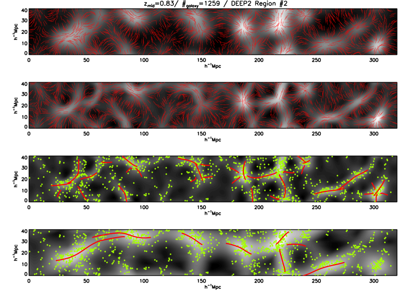
We project the galaxy distribution in each of the three DEEP2 subsamples and 33 SDSS subsamples along the short axis and measure a two-dimensional density field. We smooth each subsample with smoothing lengths $l=5$ and $10$ $h^{-1}$ Mpc and run the filament finder on them using $C=30^{\circ}l^{-1}$ and $40^{\circ}l^{-1}$ respectively. The width of filament removal is given as $K=1$ for all smoothing scales. Figure 5 shows the density field smoothed with $l=5$ $h^{-1}$ Mpc, maps of $\lambda_{1}$ and the identified filaments for DEEP2 Region 2. In the top two panels, the red bars indicate the direction of the axis of structure at each point. The axis of structure aligns with the local filamentary structure, and we identify individual filaments using the curvature criterion $C=30^{\circ}l^{-1}$ and $K=1$. In the bottom two panels of Figure 5, we show the identified filaments along with the galaxy distribution itself in green dots for the two smoothing lengths.

After excluding filaments shorter than a smoothing length $l$, we found 97 filaments in the three DEEP2 subsamples, and 958 filaments in the 33 SDSS subsamples, with smoothing length of $l=5$$h^{-1}$ Mpc. The mean total length of filaments of each subsample is $404.0$ $h^{-1}$ Mpc with a standard deviation of $29.5$ $h^{-1}$ Mpc for DEEP2, and $376.1$ $h^{-1}$ Mpc with a standard deviation of $53.8$ $h^{-1}$ Mpc for SDSS. This gives a total filament length per unit area of $3.16\times 10^{-2}$ $h$ $\rm Mpc^{-1}$ for DEEP2 subsamples, and $2.94\times 10^{-2}$ $h$ $\rm Mpc^{-1}$ for SDSS. These results are in excellent agreement; the overall length of filaments in the two cases is indistinguishable. We summarize the filamentary properties of DEEP2 and SDSS at the two smoothing length scales in Table 1.

Figure 5: The filament finder algorithm is shown in action for the subsample that corresponds to DEEP2 Region 2, a $320\times 40\times 14$ $\rm(h^{-1}Mpc)^{3}$ slice in the redshift range $0.75<z<0.92$. The smoothing length is $l=5$ $\rm h^{-1}Mpc$. (a) An inverted grayscale density map (lighter=more dense) along with a 20% random sample of bars that indicate the direction of the axis of structure at each point. (b) a grayscale map of $\lambda_{1}$ (lighter=more negative), the first eigenvalue of the second partial derivative of the density field. (c) The galaxy distribution (green dots) and filaments (in red) are shown with the grayscale map of $\lambda_{1}$ (lighter=more negative). The filaments are found with parameters $C=30^{\circ}l^{-1}$ and $K=1.0$. (d) Same as (c) but for the smoothing length $l=10$ $\rm h^{-1}Mpc$. The filaments are found with parameters $C=40^{\circ}l^{-1}$ and $K=1.0$.

Figure 6: The distribution of filaments in the DEEP2 (upper two panels) and two randomly chosen SDSS subsamples (lower two panels). The smoothing length is $l=5$ $\rm h^{-1}Mpc$ and the filaments are found with filament-finding parameters $C=30^{\circ}l^{-1}$ and $K=1.0$. The grayscale map of $\lambda_{1}$ (lighter=more negative) is shown along with the galaxy distribution (green dots) and filaments (in red).

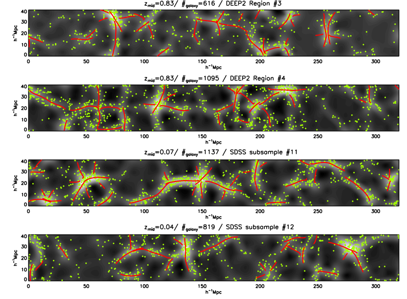
In Figure 6, we show the filaments in Region 3 and 4 of DEEP2 and two selected subsamples of SDSS. The grayscale map of $\lambda_{1}$ is shown with the identified filaments in red and the galaxy distribution in green dots. The filament distributions of DEEP2 and SDSS subsamples look qualitatively similar. We count how many galaxies lie within one smoothing length ($l$) of a filament, and thus calculate the fraction of galaxies within a smoothing length of a filament for two surveys. With smoothing length $l=5$ $\rm h^{-1}Mpc$, $81.2\pm 1.9$% of DEEP2 galaxies and $82.1\pm 0.5$% for SDSS galaxies lie within one smoothing length of filaments; the fraction of filament galaxies is almost identical in the two surveys.

Figure 7: The composite length distributions of the filaments of three DEEP2 subsamples (in blue) and 33 SDSS subsamples (in red).

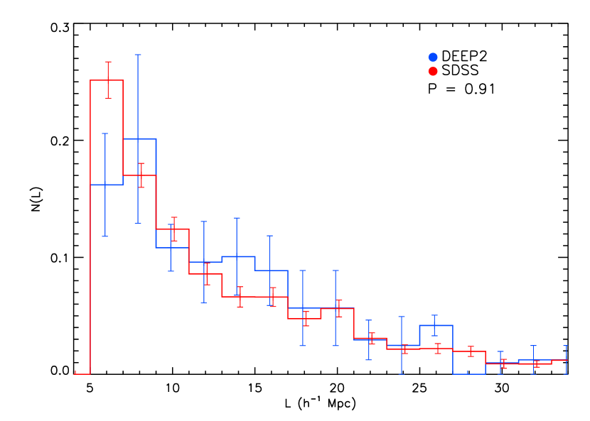
Figure 7 shows the length distribution of filament for SDSS and DEEP2 with $l=5$ $h^{-1}$ Mpc smoothing. There are too few filaments at 10 $h^{-1}$ Mpc smoothing to make a useful comparison. We derive the length distribution for each subsample and calculate the composite distribution and its error by calculating the mean and a standard deviation at each bin. The length distributions found in DEEP2 are similar to those found in SDSS. The numerical simulations in Bond (2008) showed that dark matter filaments have an exponential length distribution at large filament lengths that very closely matched that found in a Gaussian random field with the same power spectrum. This means that even if the filaments in the two galaxy distributions are at different stages of their evolution, the length distribution should be similar between the two.

Figure 8: The composite width distributions of the filaments of three DEEP2 subsamples (in blue) and 33 SDSS subsamples (in red).

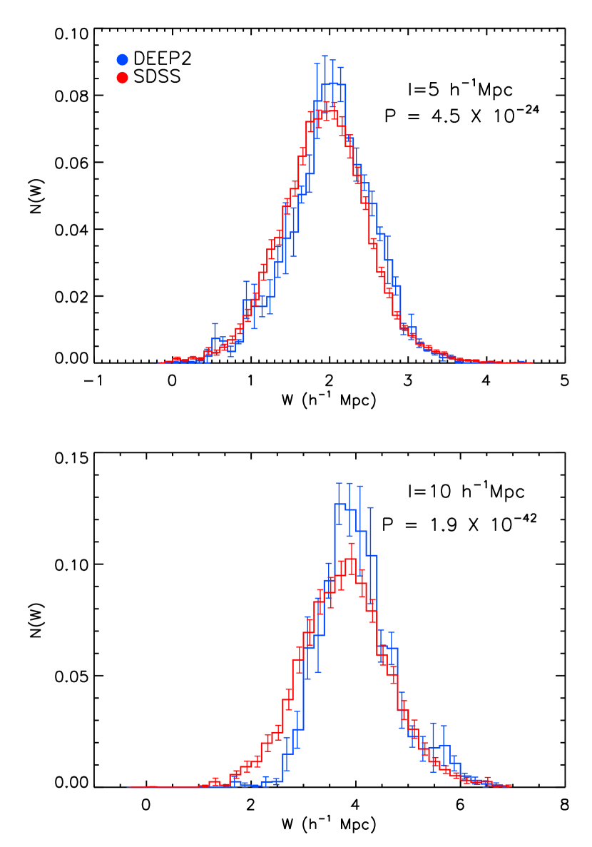
However, the width distribution of filament elements changes significantly as non-linear evolution proceeds (Paper II): it broadens and peaks at smaller widths with cosmic time, according to N-body simulations. We show the width distributions of filament elements for DEEP2 and SDSS in Figure 8 for the two smoothing lengths. We applied a K-S two-sample test to compare the two; the calculated probability that the two are drawn from the same distribution is shown in each panel in Figure 8. In both cases, the probability is negligibly small. We make Gaussian fits to the distributions to compare the two surveys. For $l=5$ $h^{-1}$ Mpc, DEEP2 has a width distribution that peaks at $\mu=2.021\pm 0.009$ $h^{-1}$ Mpc with $\sigma=0.508\pm 0.005$$h^{-1}$ Mpc, and SDSS has $\mu=1.924\pm 0.006$ $h^{-1}$ Mpc with $\sigma=0.544\pm 0.004$ $h^{-1}$ Mpc. In case of $l=10$ $h^{-1}$ Mpc, the distribution has $\mu=3.963\pm 0.0023$ $h^{-1}$ Mpc with $\sigma=0.580\pm 0.016$ $h^{-1}$ Mpc for DEEP2, and $\mu=3.802\pm 0.017$ $h^{-1}$ Mpc and $\sigma=0.808\pm 0.011$ $h^{-1}$ Mpc for SDSS. For both smoothing lengths, the filament element width distributions broaden and shift to smaller widths from $z\sim 0.8$ to $z\sim 0.1$. Figure 8 shows better match between the width distributions of SDSS and DEEP2 at high widths than low, in agreement with the simulations shown by Bond (2008). Thus, the widest filaments narrow more slowly than do the narrowest ones, as one would expect in the ellipsoidal collapse model (Zel’Dovich, 1970), in which overdensities sequentially contract along their principal axes, in order of increasing length.

5 Summary

We study the time evolution of the filament network in the galaxy distribution by comparing the filamentary structure at $z\sim 0.8$ from the Deep Extragalactic Evolutionary Probe 2 (DEEP2) Redshift Survey and those at $z\sim 0.1$ from the Sloan Digital Sky Survey (SDSS). We trace individual filaments for both surveys using SHMAFF, an algorithm which employs the Hessian matrix to trace the filamentary structures in the distribution of structure. We define three subsamples from DEEP2 and 33 subsamples from SDSS, with the same sampling and geometry, namely a box of $320\times 40\times 14$ $\rm(h^{-1}Mpc)^{3}$. We smooth the galaxy distribution with length scales of $l=5$ and $10$ $h^{-1}$ Mpc, and trace individual filaments along the axis of structure, and mark the end of filaments when the axis orientation changes more rapidly than a preset threshold of $C=30$ and $40$${}^{\circ}l^{-1}$ respectively. We found 97 filaments in DEEP2 subsamples and 957 filaments in SDSS subsamples with smoothing length $l=5$ $h^{-1}$ Mpc, and 24 filaments for DEEP2 and 230 for SDSS for $l=10$$h^{-1}$ Mpc. Thus the number of filaments per unit volume is unchanged from high to low redshift. We find that filament length distribution has not changed significantly since $z\sim 1$, however, the filament width distribution, which is sensitive to non-linear growth of structure, broadens and shifts to smaller widths for smoothing length scales of $5$ and $10$ $h^{-1}$ Mpc from $z\sim 0.8$ to $z\sim 0.1$. The evolution in the length and width distributions is consistent with predictions from a $\Lambda$CDM cosmological N-body simulation. As found in Paper II, non-linear growth of structure has a great impact on the width of filamentary structures.

We restricted our study to two-dimensional analysis due to the the geometry of the DEEP2 survey. In order to better show the filamentary evolution, however, the filamentary structures should be studied in larger volumes and analyzed in three dimensions. The next generation of galaxy surveys, which will target the early universe with larger volume and depth can open up the possibility of detailed study of filamentary structures and their evolution. These surveys include the Advanced Dark Energy Physics Telescope (ADEPT), a space-based spectroscopic survey that promises to determine the location of 100 million galaxies at $1<z<2$, the BigBOSS (Schlegel et al., 2009), a proposed ground-based wide field spectroscopic survey at $0.2<z<3.5$, and all hemisphere HI redshift surveys with the Square Kilometer Array (SKA) (Rawlings et al., 2004).

References

- Abazajian et al. (2009) Abazajian, K. N. et al., 2009, ApJS, 182, 543
- Aragón-Calvo et al. (2007) Aragón-Calvo, M. A., Jones, B. J. T., van de Weygaert, R., & van der Hulst, J. M. 2007, A&A, 474, 315
- Bharadwaj, Bhavsar & Sheth (2004) Bharadwaj, S., Bhavsar, S. P., & Sheth, J. V. 2004, ApJ, 606, 25
- Blanton et al. (2003a) Blanton M. R., et al. 2003a, ApJ, 592, 819
- Blanton et al. (2003b) Blanton, M. R., et al. 2003b, AJ, 125, 2276
- Blanton et al. (2003c) Blanton M. R., et al. 2003c, AJ, 125, 2348
- Blanton et al. (2005) Blanton M. R., et al. 2005, AJ, 129, 2562
- Bond & Myers (1996) Bond, J. R., & , Myers, S. T. 1996, ApJS, 103, 1
- Bond (2008) Bond, N. A. 2008, Ph.D. thesis, Princeton University
- Bond, Strauss, & Cen (2009) Bond, N. A., Strauss, M. A., & Cen, R. 2009, submitted to MNRAS (arXiv:0903.3601) (Paper I)
- Bond, Strauss, & Cen (2010) Bond, N. A., Strauss, M. A., & Cen, R. 2010, submitted to MNRAS (Paper II)
- Brown et al. (2003) Brown, M. J. I., Dey, A., Jannuzi, B. T., Lauer, T. R., Tiede, G. P., & Mikles, V. J. 2003, ApJ, 597, 225
- Cohen et al. (1996) Cohen, J. G., Hogg, D. W., Pahre, M. A., & Blandford, R. 1996, ApJ, 462, L9
- Coil et al. (2004a) Coil, A. et al. 2004, ApJ, 609, 525
- Coil et al. (2004b) Coil, A. et al. 2004, ApJ, 617, 765
- Coil et al. (2006) Coil, A. et al. 2006, ApJ, 638, 668
- Coil et al. (2008) Coil, A. et al. 2008, ApJ, 672, 153
- Connolly et al. (1996) Connolly, A.et al. 1996, ApJ, 473, L67
- Conroy et al. (2005) Conroy, C. et al. 2005, ApJ, 625, 990
- Davis et al. (1982) Davis, M., Huchra, J., Latham, D. W., & Tonry, J. 1982, ApJ, 253, 423
- Davis et al. (2003) Davis, M. et al. 2003, Proc. SPIE, 4834, 161
- Davis, Gerke, & Newman (2004) Davis, M., Gerke B. F., & Newman, J. A. 2004, preprint (arXiv:astro-ph/0408344)
- de Lapparent, Geller, & Huchra (1986) de Lapparent, V., Geller, M. J., & Huchra, J. P., 1986, ApJ, 302, L1
- Eriksen et al. (2004) Eriksen, H. K., Novikov, D. I., Lilje, P. B., Banday, A. J., & Górski, K. M. 2004, ApJ, 612, 64
- Faber et al. (2003) Faber, S., et al. 2003, Proc. SPIE, 4841, 1657
- Faber et al. (2007) Faber, S., et al. 2007, ApJ, 665, 265
- Forero-Romero et al. (2009) Forero-Romero, J. E., Hoffman, Y., Gottloeber, S., Klypin, A., & Yepes, G. 2009, MNRAS, 396, 1815
- Fukugita et al. (1996) Fukugita, M., Ichikawa, T., Gunn, J. E., Doi, M., Shimasaku, K., & Schneider, D. P. 1996, AJ, 111, 1748
- Gay et al. (2009) Gay, C., Pichon, C., Le Borgne, D., Teyssier, R., Sousbie, T., & Devriendt, J. 2009, arXiv:0910.1728
- Geller & Huchra (1989) Geller, M. J., & Huchra, J. P. 1989, Science, 246, 897
- Giavalisco et al. (1998) Giavalisco, M. et al. 1998, ApJ, 503, 543
- Gott et al. (2005) Gott, J. R., III, et al. 2005, ApJ, 624, 463
- Gunn et al. (1998) Gunn, J. E., et al. 1998, AJ, 116, 3040
- Gunn et al. (2006) Gunn, J. E., et al. 2006, AJ, 131, 2332
- Ivezić et al. (2004) Ivezić, Ž., et al. 2004, Astron. Nachr., 325, 583
- Lacoste et al. (2005) Lacoste, C., Descombes, X., & Zerubia, J. 2005, IEEE Trans. Pattern Analysis and Machine Intelligence, 27, 1568
- Le Fèvre et al. (2005) Le Fèvre, O., et al. 2005, A&A, 439, 877
- Meneux et al. (2006) Meneux, B. et al. 2006, A&A, 452, 387
- Moody, Turner & Gott (1983) Moody, J. E., Turner, E. L., & Gott, J. R. 1983, ApJ, 273, 16
- Novikov, Colombi & Doré (2006) Novikov, D., Colombi, S., & Doré, O. 2006, MNRAS, 366, 1201
- Ouchi et al. (2004) Ouchi, M. et al. 2004, ApJ, 611, 685
- Phleps & Meisenheimer (2003) Phleps, S. & Meisenheimer, K. 2003, A&A, 407, 855
- Rawlings et al. (2004) Rawlings, S. et al. 2004, arXiv:astro-ph/0409479
- Schechter (1976) Schechter, P. 1976, ApJ, 203, 297
- Schlegel et al. (2009) Schlegel, D. J. et al. 2009, arXiv:0904.0468
- Smith et al. (2002) Smith J. A. et al. 2002, AJ, 123, 2121
- Sousbie et al. (2008a) Sousbie, T., Pichon, C., Colombi, S., Novikov, D., & Pogosyan, D. 2008a, MNRAS, 383, 1655
- Sousbie et al. (2008b) Sousbie, T., Pichon, C., Courtois, H., Colombi, S., & Novikov, D. 2008b, ApJ, 672, L1
- Soubie, Colombi & Pichon (2009) Sousbie, T., Colombi, S., & Pichon, C. 2009, MNRAS, 393, 457
- Stoica et al. (2005) Stoica, R. S., Martinez, V. J., Mateu, J., & Saar, E. 2005, ApJ, 434, 423
- Stoica et al. (2007) Stoica, R. S., Martinez, V. J., & Saar, E. 2007, Journal of the Royal Statistical Society : Series C (Applied Statistics), 55, 189
- Stoughton et al. (2002) Stoughton C., et al. 2002, AJ, 123, 485
- Strauss et al. (2002) Strauss, M A., et al. 2002, AJ, 124, 1810
- Willmer et al. (2006) Willmer, C. N. A. et al. 2006, ApJ, 647, 853
- York et al. (2000) York D. G. et al. 2000, AJ, 120, 1579
- Zel’Dovich (1970) Zel’Dovich Y. B. 1970, A&A, 5, 84