Universal Regularizers For Robust Sparse Coding and Modeling
Abstract
Sparse data models, where data is assumed to be well represented as a linear combination of a few elements from a dictionary, have gained considerable attention in recent years, and their use has led to state-of-the-art results in many signal and image processing tasks. It is now well understood that the choice of the sparsity regularization term is critical in the success of such models. Based on a codelength minimization interpretation of sparse coding, and using tools from universal coding theory, we propose a framework for designing sparsity regularization terms which have theoretical and practical advantages when compared to the more standard or ones. The presentation of the framework and theoretical foundations is complemented with examples that show its practical advantages in image denoising, zooming and classification.
I Introduction
Sparse modeling calls for constructing a succinct representation of some data as a combination of a few typical patterns (atoms) learned from the data itself. Significant contributions to the theory and practice of learning such collections of atoms (usually called dictionaries or codebooks), e.g., [1, 14, 33], and of representing the actual data in terms of them, e.g., [8, 11, 12], have been developed in recent years, leading to state-of-the-art results in many signal and image processing tasks [24, 26, 27, 34]. We refer the reader for example to [4] for a recent review on the subject.
A critical component of sparse modeling is the actual sparsity of the representation, which is controlled by a regularization term (regularizer for short) and its associated parameters. The choice of the functional form of the regularizer and its parameters is a challenging task. Several solutions to this problem have been proposed in the literature, ranging from the automatic tuning of the parameters [20] to Bayesian models, where these parameters are themselves considered as random variables [17, 20, 51]. In this work we adopt the interpretation of sparse coding as a codelength minimization problem. This is a natural and objective method for assessing the quality of a statistical model for describing given data, and which is based on the Minimum Description Length (MDL) principle [37]. In this framework, the regularization term in the sparse coding formulation is interpreted as the cost in bits of describing the sparse linear coefficients used to reconstruct the data. Several works on image coding using this approach were developed in the 1990’s under the name of “complexity-based” or “compression-based” coding, following the popularization of MDL as a powerful statistical modeling tool [9, 31, 40]. The focus on these early works was in denoising using wavelet basis, using either generic asymptotic results from MDL or fixed probability models, in order to compute the description length of the coefficients. A later, major breakthrough in MDL theory was the adoption of universal coding tools to compute optimal codelengths. In this work, we improve and extend on previous results in this line of work by designing regularization terms based on such universal codes for image coefficients, meaning that the codelengths obtained when encoding the coefficients of any (natural) image with such codes will be close to the shortest codelengths that can be obtained with any model fitted specifically for that particular instance of coefficients. The resulting framework not only formalizes sparse coding from the MDL and universal coding perspectives but also leads to a family of universal regularizers which we show to consistently improve results in image processing tasks such as denoising and classification. These models also enjoy several desirable theoretical and practical properties such as statistical consistency (in certain cases), improved robustness to outliers in the data, and improved sparse signal recovery (e.g., decoding of sparse signals from a compressive sensing point of view [5]) when compared with the traditional and -based techniques in practice. These models also yield to the use of a simple and efficient optimization technique for solving the corresponding sparse coding problems as a series of weighted subproblems, which in turn, can be solved with off-the-shelf algorithms such as LARS [12] or IST [11]. Details are given in the sequel.
Finally, we apply our universal regularizers not only for coding using fixed dictionaries, but also for learning the dictionaries themselves, leading to further improvements in all the aforementioned tasks.
The remainder of this paper is organized as follows: in Section II we introduce the standard framework of sparse modeling. Section III is dedicated to the derivation of our proposed universal sparse modeling framework, while Section IV deals with its implementation. Section V presents experimental results showing the practical benefits of the proposed framework in image denoising, zooming and classification tasks. Concluding remarks are given in Section VI.
II Sparse modeling and the need for better models
Let be a set of column data samples , a dictionary of column atoms , and , a set of reconstruction coefficients such that . We use to denote the -th row of , the coefficients associated to the -th atom in . For each we define the active set of as , and as its cardinality. The goal of sparse modeling is to design a dictionary such that for all or most data samples , there exists a coefficients vector such that and is small (usually below some threshold ). Formally, we would like to solve the following problem
| (1) |
where is a regularization term which induces sparsity in the columns of the solution . Usually the constraint , is added, since otherwise we can always decrease the cost function arbitrarily by multiplying by a large constant and dividing by the same constant. When is fixed, the problem of finding a sparse for each sample is called sparse coding,
| (2) |
Among possible choices of are the pseudo-norm, , and the norm. The former tries to solve directly for the sparsest , but since it is non-convex, it is commonly replaced by the norm, which is its closest convex approximation. Furthermore, under certain conditions on (fixed) and the sparsity of , the solutions to the and -based sparse coding problems coincide (see for example [5]). The problem (1) is also usually formulated in Lagrangian form,
| (3) |
along with its respective sparse coding problem when is fixed,
| (4) |
Even when the regularizer is convex, the sparse modeling problem, in any of its forms, is jointly non-convex in . Therefore, the standard approach to find an approximate solution is to use alternate minimization: starting with an initial dictionary , we minimize (3) alternatively in via (2) or (4) (sparse coding step), and (dictionary update step). The sparse coding step can be solved efficiently when using for example ist [11] or lars [12], or with omp [28] when . The dictionary update step can be done using for example mod [14] or k-svd [1].
II-A Interpretations of the sparse coding problem
We now turn our attention to the sparse coding problem: given a fixed dictionary , for each sample vector , compute the sparsest vector of coefficients that yields a good approximation of . The sparse coding problem admits several interpretations. What follows is a summary of these interpretations and the insights that they provide into the properties of the sparse models that are relevant to our derivation.
II-A1 Model selection in statistics
Using the norm as in (4) is known in the statistics community as the Akaike’s Information Criterion (aic) when , or the Bayes Information Criterion (bic) when , two popular forms of model selection (see [22, Chapter 7]). In this context, the regularizer was introduced in [43], again as a convex approximation of the above model selection methods, and is commonly known (either in its constrained or Lagrangian forms) as the Lasso. Note however that, in the regression interpretation of (4), the role of and is very different.
II-A2 Maximum a posteriori
Another interpretation of (4) is that of a maximum a posteriori (map) estimation of in the logarithmic scale, that is
| (5) | |||||
where the observed samples are assumed to be contaminated with additive, zero mean, iid Gaussian noise with variance , and a prior probability model on with the form is considered. The energy term in Equation (4) follows by plugging the previous two probability models into (5) and factorizing into . According to (5), the regularizer corresponds to an iid Laplacian prior with mean and inverse-scale parameter , , which has a special meaning in signal processing tasks such as image or audio compression. This is due to the widely accepted fact that representation coefficients derived from predictive coding of continuous-valued signals, and, more generally, responses from zero-mean filters, are well modeled using Laplacian distributions. For example, for the special case of dct coefficients of image patches, an analytical study of this phenomenon is provided in [25], along with further references on the subject.
II-A3 Codelength minimization
Sparse coding, in all its forms, has yet another important interpretation. Suppose that we have a fixed dictionary and that we want to use it to compress an image, either losslessly by encoding the reconstruction coefficients and the residual , or in a lossy manner, by obtaining a good approximation and encoding only . Consider for example the latter case. Most modern compression schemes consist of two parts: a probability assignment stage, where the data, in this case , is assigned a probability , and an encoding stage, where a code of length bits is assigned to the data given its probability, so that is as short as possible. The techniques known as Arithmetic and Huffman coding provide the best possible solution for the encoding step, which is to approximate the Shannon ideal codelength [10, Chapter 5]. Therefore, modern compression theory deals with finding the coefficients that maximize , or, equivalently, that minimize . Now, to encode lossily, we obtain coefficients such that each data sample is approximated up to a certain distortion , . Therefore, given a model for a vector of reconstruction coefficients, and assuming that we encode each sample independently, the optimum vector of coefficients for each sample will be the solution to the optimization problem
| (6) |
which, for the choice coincides with the error constrained sparse coding problem (2). Suppose now that we want lossless compression. In this case we also need to encode the reconstruction residual . Since , the combined codelength will be
| (7) |
Therefore, obtaining the best coefficients amounts to solving , which is precisely the map formulation of (5), which in turn, for proper choices of and , leads to the Lagrangian form of sparse coding (4).111Laplacian models, as well as Gaussian models, are probability distributions over , characterized by continuous probability density functions, , . If the reconstruction coefficients are considered real numbers, under any of these distributions, any instance of will have measure , that is, . In order to use such distributions as our models for the data, we assume that the coefficients in are quantized to a precision , small enough for the density function to be approximately constant in any interval , so that we can approximate . Under these assumptions, , and the effect of on the codelength produced by any model is the same. Therefore, we will omit in the sequel, and treat density functions and probability distributions interchangeably as . Of course, in real compression applications, needs to be tuned.
As one can see, the codelength interpretation of sparse coding is able to unify and interpret both the constrained and unconstrained formulations into one consistent framework. Furthermore, this framework offers a natural and objective measure for comparing the quality of different models and in terms of the codelengths obtained.
II-A4 Remarks on related work
As mentioned in the introduction, the codelength interpretation of signal coding was already studied in the context of orthogonal wavelet-based denoising. An early example of this line of work considers a regularization term which uses the Shannon Entropy function to give a measure of the sparsity of the solution [9]. However, the Entropy function is not used as measure of the ideal codelength for describing the coefficients, but as a measure of the sparsity (actually, group sparsity) of the solution. The MDL principle was applied to the signal estimation problem in [40]. In this case, the codelength term includes the description of both the location and the magnitude of the nonzero coefficients. Although a pioneering effort, the model assumed in [40] for the coefficient magnitude is a uniform distribution on , which does not exploit a priori knowledge of image coefficient statistics, and the description of the support is slightly wasteful. Furthermore, the codelength expression used is an asymptotic result, actually equivalent to bic (see Section II-A1) which can be misleading when working with small sample sizes, such as when encoding small image patches, as in current state of the art image processing applications. The uniform distribution was later replaced by the universal code for integers [38] in [31]. However, as in [40], the model is so general that it does not perform well for the specific case of coefficients arising from image decompositions, leading to poor results. In contrast, our models are derived following a careful analysis of image coefficient statistics. Finally, probability models suitable to image coefficient statistics of the form (known as generalized Gaussians) were applied to the MDL-based signal coding and estimation framework in [31]. The justification for such models is based on the empirical observation that sparse coefficients statistics exhibit “heavy tails” (see next section). However, the choice is ad hoc and no optimality criterion is available to compare it with other possibilities. Moreover, there is no closed form solution for performing parameter estimation on such family of models, requiring numerical optimization techniques. In Section III, we derive a number of probability models for which parameter estimation can be computed efficiently in closed form, and which are guaranteed to optimally describe image coefficients.
II-B The need for a better model

As explained in the previous subsection, the use of the regularizer implies that all the coefficients in share the same Laplacian parameter . However, as noted in [25] and references therein, the empirical variance of coefficients associated to different atoms, that is, of the different rows of , varies greatly with . This is clearly seen in Figures 1(a-c), which show the empirical distribution of dct coefficients of patches. As the variance of a Laplacian is , different variances indicate different underlying . The histogram of the set of estimated Laplacian parameters for each row , Figure 1(d), shows that this is indeed the case, with significant occurrences of values of in a range of to .
The straightforward modification suggested by this phenomenon is to use a model where each row of has its own weight associated to it, leading to a weighted regularizer. However, from a modeling perspective, this results in parameters to be adjusted instead of just one, which often results in poor generalization properties. For example, in the cases studied in Section V, even with thousands of images for learning these parameters, the results of applying the learned model to new images were always significantly worse (over 1dB in estimation problems) when compared to those obtained using simpler models such as an unweighted . 222Note that this is the case when the weights are found by maximum likelihood. Other applications of weighted regularizers, using other types of weighting strategies, are known to improve over -based ones for certain applications (see e.g. [51]). One reason for this failure may be that real images, as well as other types of signals such as audio samples, are far from stationary. In this case, even if each atom is associated to its own (), the optimal value of can have significant local variations at different positions or times. This effect is shown in Figure 1(e), where, for each , each was re-estimated several times using samples from different regions of an image, and the histogram of the different estimated values of was computed. Here again we used the dct basis as the dictionary .
The need for a flexible model which at the same time has a small number of parameters leads naturally to Bayesian formulations where the different possible are “marginalized out” by imposing an hyper-prior distribution on , sampling using its posterior distribution, and then averaging the estimates obtained with the sampled sparse-coding problems. Examples of this recent line of work, and the closely related Bayesian Compressive Sensing, are developed for example in [23, 44, 49, 48]. Despite of its promising results, the Bayesian approach is often criticized due to the potentially expensive sampling process (something which can be reduced for certain choices of the priors involved [23]), arbitrariness in the choice of the priors, and lack of proper theoretical justification for the proposed models [48].
In this work we pursue the same goal of deriving a more flexible and accurate sparse model than the traditional ones, while avoiding an increase in the number of parameters and the burden of possibly solving several sampled instances of the sparse coding problem. For this, we deploy tools from the very successful information-theoretic field of universal coding, which is an extension of the compression scenario summarized above in Section II-A, when the probability model for the data to be described is itself unknown and has to be described as well.
III Universal models for sparse coding
Following the discussion in the preceding section, we now have several possible scenarios to deal with. First, we may still want to consider a single value of to work well for all the coefficients in , and try to design a sparse coding scheme that does not depend on prior knowledge on the value of . Secondly, we can consider an independent (but not identically distributed) Laplacian model where the underlying parameter can be different for each atom , . In the most extreme scenario, we can consider each single coefficient in to have its own unknown underlying and yet, we would like to encode each of these coefficients (almost) as if we knew its hidden parameter.
The first two scenarios are the ones which fit the original purpose of universal coding theory [29], which is the design of optimal codes for data whose probability models are unknown, and the models themselves are to be encoded as well in the compressed representation.
Now we develop the basic ideas and techniques of universal coding applied to the first scenario, where the problem is to describe as an iid Laplacian with unknown parameter . Assuming a known parametric form for the prior, with unknown parameter , leads to the concept of a model class. In our case, we consider the class of all iid Laplacian models over , where
and . The goal of universal coding is to find a probability model which can fit as well as the model in that best fits after having observed it. A model with this property is called universal (with respect to the model ).
For simplicity, in the following discussion we consider the coefficient matrix to be arranged as a single long column vector of length , . We also use the letter without sub-index to denote the value of a random variable representing coefficient values.
First we need to define a criterion for comparing the fitting quality of different models. In universal coding theory this is done in terms of the codelengths required by each model to describe .
If the model consists of a single probability distribution , we know from Section II-A3 that the optimum codelength corresponds to . Moreover, this relationship defines a one-to-one correspondence between distributions and codelengths, so that for any coding scheme , . Now suppose that we are restricted to a class of models , and that we need choose the model that assigns the shortest codelength to a particular instance of . We then have that is the model in that assigns the maximum probability to . For a class parametrized by , this corresponds to , where is the maximum likelihood estimator (mle) of the model class parameter given (we will usually omit the argument and just write ). Unfortunately, we also need to include the value of in the description of for the decoder to be able to reconstruct it from the code . Thus, we have that any model inducing valid codelengths will have . The overhead of with respect to is known as the codelength regret,
A model (or, more precisely, a sequence of models, one for each data length ) is called universal if grows sublinearly in for all possible realizations of , that is so that the codelength regret with respect to the mle becomes asymptotically negligible.
There are a number of ways to construct universal probability models. The simplest one is the so called two-part code, where the data is described in two parts. The first part describes the optimal parameter and the second part describes the data according to the model with the value of the estimated parameter , . For uncountable parameter spaces , such as a compact subset of , the value of has to be quantized in order to be described with a finite number of bits . We call the quantized parameter . The regret for this model is thus
The key for this model to be universal is in the choice of the quantization step for the parameter , so that both its description , and the difference , grow sublinearly. This can be achieved by letting the quantization step shrink as [37], thus requiring bits to describe each dimension of . This gives us a total regret for two-part codes which grows as , where is the dimension of the parameter space .
Another important universal code is the so called Normalized Maximum Likelihood (nml) [42]. In this case the universal model corresponds to the model that minimizes the worst case regret,
which can be written in closed form as , where the normalization constant
is the value of the minimax regret and depends only on and the length of the data .333The minimax optimality of derives from the fact that it defines a complete uniquely decodable code for all data of length , that is, it satisfies the Kraft inequality with equality. Since every uniquely decodable code with lengths must satisfy the Kraft inequality (see [10, Chapter 5]), if there exists a value of such that (that is ), then there exists a vector for which for the Kraft inequality to hold. Therefore the regret of for is necessarily greater than , which shows that is minimax optimal. Note that the nml model requires to be finite, something which is often not the case.
The two previous examples are good for assigning a probability to coefficients that have already been computed, but they cannot be used as a model for computing the coefficients themselves since they depend on having observed them in the first place. For this and other reasons that will become clearer later, we concentrate our work on a third important family of universal codes derived from the so called mixture models (also called Bayesian mixtures). In a mixture model, is a convex mixture of all the models in , indexed by the model parameter , , where specifies the weight of each model. Being a convex mixture implies that and , thus is itself a probability measure over . We will restrict ourselves to the particular case when is considered a sequence of independent random variables,444More sophisticated models which include dependencies between the elements of are out of the scope of this work.
| (8) |
where the mixing function can be different for each sample . An important particular case of this scheme is the so called Sequential Bayes code, in which is computed sequentially as a posterior distribution based on previously observed samples, that is [21, Chapter 6]. In this work, for simplicity, we restrict ourselves to the case where is the same for all . The result is an iid model where the probability of each sample is a mixture of some probability measure over ,
| (9) |
A well known result for iid mixture (Bayesian) codes states that their asymptotic regret is , thus stating their universality, as long as the weighting function is positive, continuous and unimodal over (see for example [21, Theorem 8.1],[41]). This gives us great flexibility on the choice of a weighting function that guarantees universality. Of course, the results are asymptotic and the terms can be large, so that the choice of can have practical impact for small sample sizes.
In the following discussion we derive several iid mixture models for the Laplacian model class . For this purpose, it will be convenient to consider the corresponding one-sided counterpart of the Laplacian, which is the exponential distribution over the absolute value of the coefficients, , and then symmetrize back to obtain the final distribution over the signed coefficients .
III-A The conjugate prior
In general, (9) can be computed in closed form if is the conjugate prior of . When is an exponential (one-sided Laplacian), the conjugate prior is the Gamma distribution,
where and are its shape and scale parameters respectively. Plugging this in (9) we obtain the Mixture of exponentials model (moe), which has the following form (see Appendix Derivation of the MOE model for the full derivation),
| (10) |
With some abuse of notation, we will also denote the symmetric distribution on as moe,
| (11) |
Although the resulting prior has two parameters to deal with instead of one, we know from universal coding theory that, in principle, any choice of and will give us a model whose codelength regret is asymptotically small.
Furthermore, being iid models, each coefficient of itself is modeled as a mixture of exponentials, which makes the resulting model over very well suited to the most flexible scenario where the “underlying” can be different for each . In Section V-B we will show that a single moe distribution can fit each of the rows of better than separate Laplacian distributions fine-tuned to these rows, with a total of parameters to be estimated. Thus, not only we can deal with one single unknown , but we can actually achieve maximum flexibility with only two parameters ( and ). This property is particular of the mixture models, and does not apply to the other universal models presented.
Finally, if desired, both and can be easily estimated using the method of moments (see Appendix Derivation of the MOE model). Given sample estimates of the first and second non-central moments, and , we have that
| (12) |
When the moe prior is plugged into (5) instead of the standard Laplacian, the following new sparse coding formulation is obtained,
| (13) |
where . An example of the moe regularizer, and the thresholding function it induces, is shown in Figure 2 (center column) for . Smooth, differentiable non-convex regularizers such as the one in in (13) have become a mainstream robust alternative to the norm in statistics [16, 51]. Furthermore, it has been shown that the use of such regularizers in regression leads to consistent estimators which are able to identify the relevant variables in a regression model (oracle property) [16]. This is not always the case for the regularizer, as was proved in [51]. The moe regularizer has also been recently proposed in the context of compressive sensing [6], where it is conjectured to be better than the -term at recovering sparse signals in compressive sensing applications.555In [6], the logarithmic regularizer arises from approximating the pseudo-norm as an -normalized element-wise sum, without the insight and theoretical foundation here reported. This conjecture was partially confirmed recently for non-convex regularizers of the form with in [39, 18], and for a more general family of non-convex regularizers including the one in (13) in [47]. In all cases, it was shown that the conditions on the sensing matrix (here ) can be significantly relaxed to guarantee exact recovery if non-convex regularizers are used instead of the norm, provided that the exact solution to the non-convex optimization problem can be computed. In practice, this regularizer is being used with success in a number of applications here and in [7, 46].666While these works support the use of such non-convex regularizers, none of them formally derives them using the universal coding framework as in this paper. Our experimental results in Section V provide further evidence on the benefits of the use of non-convex regularizers, leading to a much improved recovery accuracy of sparse coefficients compared to and . We also show in Section V that the moe prior is much more accurate than the standard Laplacian to model the distribution of reconstruction coefficients drawn from a large database of image patches. We also show in Section V how these improvements lead to better results in applications such as image estimation and classification.
III-B The Jeffreys prior
The Jeffreys prior for a parametric model class , is defined as
| (14) |
where is the determinant of the Fisher information matrix
| (15) |
The Jeffreys prior is well known in Bayesian theory due to three important properties: it virtually eliminates the hyper-parameters of the model, it is invariant to the original parametrization of the distribution, and it is a “non-informative prior,” meaning that it represents well the lack of prior information on the unknown parameter [3]. It turns out that, for quite different reasons, the Jeffreys prior is also of paramount importance in the theory of universal coding. For instance, it has been shown in [2] that the worst case regret of the mixture code obtained using the Jeffreys prior approaches that of the nml as the number of samples grows. Thus, by using Jeffreys, one can attain the minimum worst case regret asymptotically, while retaining the advantages of a mixture (not needing hindsight of ), which in our case means to be able to use it as a model for computing via sparse coding.
For the exponential distribution we have that . Clearly, if we let , the integral in (14) evaluates to . Therefore, in order to obtain a proper integral, we need to exclude and from (note that this was not needed for the conjugate prior). We choose to define , , leading to
The resulting mixture, after being symmetrized around , has the following form (see Appendix Derivation of the constrained Jeffreys (JOE) model):
| (16) |
We refer to this prior as a Jeffreys mixture of exponentials (joe), and again overload this acronym to refer to the symmetric case as well. Note that although is not defined for , its limit when is finite and evaluates to . Thus, by defining , we obtain a prior that is well defined and continuous for all . When plugged into (5), we get the joe-based sparse coding formulation,
| (17) |
where, according to the convention just defined for , we define . According to the map interpretation we have that , coming from the Gaussian assumption on the approximation error as explained in Section II-A.
As with moe, the joe-based regularizer, , is continuous and differentiable in , and its derivative converges to a finite value at zero, . As we will see later in Section IV, these properties are important to guarantee the convergence of sparse coding algorithms using non-convex priors. Note from (17) that we can rewrite the joe regularizer as
so that for sufficiently large , , , and we have that . Thus, for large , the joe regularizer behaves like with . In terms of the probability model, this means that the tails of the joe mixture behave like a Laplacian with , with the region where this happens determined by the value of . The fact that the non-convex region of is confined to a neighborhood around could help to avoid falling in bad local minima during the optimization (see Section IV for more details on the optimization aspects). Finally, although having Laplacian tails means that the estimated will be biased [16], the sharper peak at allows us to perform a more aggressive thresholding of small values, without excessively clipping large coefficients, which leads to the typical over-smoothing of signals recovered using an regularizer. See Figure 2 (rightmost column) for an example regularizer based on joe with parameters , and the thresholding function it induces.

The joe regularizer has two hyper-parameters which define and that, in principle, need to be tuned. One possibility is to choose and based on the physical properties of the data to be modeled, so that the possible values of never fall outside of the range . For example, in modeling patches from grayscale images with a limited dynamic range of in a dct basis, the maximum variance of the coefficients can never exceed . The same is true for the minimum variance, which is defined by the quantization noise.
Having said this, in practice it is advantageous to adjust to the data at hand. In this case, although no closed form solutions exist for estimating using mle or the method of moments, standard optimization techniques can be easily applied to obtain them. See Appendix Derivation of the constrained Jeffreys (JOE) model for details.
III-C The conditional Jeffreys
A recent approach to deal with the case when the integral over in the Jeffreys prior is improper, is the conditional Jeffreys [21, Chapter 11]. The idea is to construct a proper prior, based on the improper Jeffreys prior and the first few samples of , , and then use it for the remaining data. The key observation is that although the normalizing integral in the Jeffreys prior is improper, the unnormalized prior can be used as a measure to weight ,
| (18) |
It turns out that the integral in (18) usually becomes proper for small in the order of . In our case we have that for any , the resulting prior is a distribution with and (see Appendix Derivation of the conditional Jeffreys (CMOE) model for details). Therefore, using the conditional Jeffreys prior in the mixture leads to a particular instance of moe, which we denote by cmoe (although the functional form is identical to moe), where the Gamma parameters and are automatically selected from the data. This may explain in part why the Gamma prior performs so well in practice, as we will see in Section V.
Furthermore, we observe that the value of obtained with this approach () coincides with the one estimated using the method of moments for moe if the in moe is fixed to . Indeed, if computed from samples, the method of moments for moe gives , with , which gives us . It turns out in practice that the value of estimated using the method of moments gives a value between and for the type of data that we deal with (see Section V), which is just above the minimum acceptable value for the cmoe prior to be defined, which is . This justifies our choice of when applying cmoe in practice.
As becomes large, so does , and the Gamma prior obtained with this method converges to a Kronecker delta at the mean value of the Gamma distribution, . Consequently, when , the mixture will be close to . Moreover, from the definition of and we have that is exactly the mle of for the Laplacian distribution. Thus, for large , the conditional Jeffreys method approaches the mle Laplacian model.
Although from a universal coding point of view this is not a problem, for large the conditional Jeffreys model will loose its flexibility to deal with the case when different coefficients in have different underlying . On the other hand, a small can lead to a prior that is overfitted to the local properties of the first samples, which for non-stationary data such as image patches, can be problematic. Ultimately, defines a trade-off between the degree of flexibility and the accuracy of the resulting model.
IV Optimization and implementation details
All of the mixture models discussed so far yield non-convex regularizers, rendering the sparse coding problem non-convex in . It turns out however that these regularizers satisfy certain conditions which make the resulting sparse coding optimization well suited to be approximated using a sequence of successive convex sparse coding problems, a technique known as Local Linear Approximation (lla) [52] (see also [46, 19] for alternative optimization techniques for such non-convex sparse coding problems). In a nutshell, suppose we need to obtain an approximate solution to
| (19) |
where is a non-convex function over . At each lla iteration, we compute by doing a first order expansion of around the elements of the current estimate ,
and solving the convex weighted problem that results after discarding the constant terms ,
| (20) | |||||
where we have defined . If is continuous in , and right-continuous and finite at , then the lla algorithm converges to a stationary point of (19) [51]. These conditions are met for both the moe and joe regularizers. Although, for the joe prior, the derivative is not defined at , it converges to the limit when , which is well defined for . If , the joe mixing function is a Kronecker delta and the prior becomes a Laplacian with parameter . Therefore we have that for all of the mixture models studied, the lla method converges to a stationary point. In practice, we have observed that iterations are enough to converge. Thus, the cost of sparse coding, with the proposed non-convex regularizers, is at most times that of a single sparse coding, and could be less in practice if warm restarts are used to begin each iteration.
Of course we need a starting point , and, being a non-convex problem, this choice will influence the approximation that we obtain. One reasonable choice, used in this work, is to define , where is a scalar so that , that is, so that the first sparse coding corresponds to a Laplacian regularizer whose parameter is the average value of as given by the mixing prior .
Finally, note that although the discussion here has revolved around the Lagrangian formulation to sparse coding of (4), this technique is also applicable to the constrained formulation of sparse-coding given by Equation (1) for a fixed dictionary .
Expected approximation error: Since we are solving a convex approximation to the actual target optimization problem, it is of interest to know how good this approximation is in terms of the original cost function. To give an idea of this, after an approximate solution is obtained, we compute the expected value of the difference between the true and approximate regularization term values. The expectation is taken, naturally, in terms of the assumed distribution of the coefficients in . Since the regularizers are separable, we can compute the error in a separable way as an expectation over each -th coefficient, , where is the approximation of around the final estimate of . For the case of , the expression obtained is (see Appendix)
In the moe case, for and fixed, the minimum of occurs when . We also have .
The function can be evaluated on each coefficient of to give an idea of its quality. For example, in the experiments from Section V, we obtained an average value of , which lies between and . Depending on the experiment, this represents 6% to 7% of the total sparse coding cost function value, showing the efficiency of the proposed optimization.
Comments on parameter estimation: All the universal models presented so far, with the exception of the conditional Jeffreys, depend on hyper-parameters which in principle should be tuned for optimal performance (remember that they do not influence the universality of the model). If tuning is needed, it is important to remember that the proposed universal models are intended for reconstruction coefficients of clean data, and thus their hyper-parameters should be computed from statistics of clean data, or either by compensating the distortion in the statistics caused by noise (see for example [30]). Finally, note that when is linearly dependent and , the coefficients matrix resulting from an exact reconstruction of will have many zeroes which are not properly explained by any continuous distribution such as a Laplacian. We sidestep this issue by computing the statistics only from the non-zero coefficients in . Dealing properly with the case is beyond the scope of this work.
V Experimental results
In the following experiments, the testing data are patches drawn from the Pascal VOC2006 testing subset,777http://pascallin.ecs.soton.ac.uk/challenges/VOC/databases.html#VOC2006 which are high quality rgb images with 8 bits per channel. For the experiments, we converted the 2600 images to grayscale by averaging the channels, and scaled the dynamic range to lie in the interval. Similar results to those shown here are also obtained for other patch sizes.
V-A Dictionary learning
For the experiments that follow, unless otherwise stated, we use a “global” overcomplete dictionary with atoms trained on the full VOC2006 training subset using the method described in [35, 36], which seeks to minimize the following cost during training,888While we could have used off-the-shelf dictionaries such as dct in order to test our universal sparse coding framework, it is important to use dictionaries that lead to the state-of-the-art results in order to show the additional potential improvement of our proposed regularizers.
| (21) |
where denotes Frobenius norm. The additional term, , encourages incoherence in the learned dictionary, that is, it forces the atoms to be as orthogonal as possible. Dictionaries with lower coherence are well known to have several theoretical advantages such as improved ability to recover sparse signals [11, 45], and faster and better convergence to the solution of the sparse coding problems (1) and (3) [13]. Furthermore, in [35] it was shown that adding incoherence leads to improvements in a variety of sparse modeling applications, including the ones discussed below.
V-B moe as a prior for sparse coding coefficients
We begin by comparing the performance of the Laplacian and moe priors for fitting a single global distribution to the whole matrix . We compute using (1) with and then, following the discussion in Section IV, restrict our study to the nonzero elements of .
The empirical distribution of is plotted in Figure 3(a), along with the best fitting Laplacian, moe, joe, and a particularly good example of the conditional Jeffreys (cmoe) distributions.999To compute the empirical distribution, we quantized the elements of uniformly in steps of , which for the amount of data available, gives us enough detail and at the same time reliable statistics for all the quantized values. The mle for the Laplacian fit is (here is the number of nonzero elements in ). For moe, using (12), we obtained and . For joe, and . According to the discussion in Section III-C, we used the value obtained using the method of moments for moe as a hint for choosing (), yielding , which coincides with the obtained using the method of moments. As observed in Figure 3(a), in all cases the proposed mixture models fit the data better, significantly better for both Gamma-based mixtures, moe and cmoe, and slightly better for joe. This is further confirmed by the Kullback-Leibler divergence (kld) obtained in each case. Note that joe fails to significantly improve on the Laplacian mode due to the excessively large estimated range . In this sense, it is clear that the joe model is very sensitive to its hyper-parameters, and a better and more robust estimation would be needed for it to be useful in practice.
Given these results, hereafter we concentrate on the best case which is the moe prior (which, as detailed above, can be derived from the conditional Jeffreys as well, thus representing both approaches).
From Figure 1(e) we know that the optimal varies locally across different regions, thus, we expect the mixture models to perform well also on a per-atom basis. This is confirmed in Figure 3(b), where we show, for each row , the difference in kld between the globally fitted moe distribution and the best per-atom fitted moe, the globally fitted Laplacian, and the per-atom fitted Laplacians respectively. As can be observed, the kld obtained with the global moe is significantly smaller than the global Laplacian in all cases, and even the per-atom Laplacians in most of the cases. This shows that moe, with only two parameters (which can be easily estimated, as detailed in the text), is a much better model than Laplacians (requiring critical parameters) fitted specifically to the coefficients associated to each atom. Whether these modeling improvements have a practical impact is explored in the next experiments.
V-C Recovery of noisy sparse signals
Here we compare the active set recovery properties of the moe prior, with those of the -based one, on data for which the sparsity assumption holds exactly for all . To this end, we obtain sparse approximations to each sample using the -based Orthogonal Matching Pursuit algorithm (omp) on [28], and record the resulting active sets as ground truth. The data is then contaminated with additive Gaussian noise of variance and the recovery is performed by solving (1) for with and either the or the moe-based regularizer for . We use , which is a standard value in denoising applications (see for example [27]).
For each sample , we measure the error of each method in recovering the active set as the Hamming distance between the true and estimated support of the corresponding reconstruction coefficients. The accuracy of the method is then given as the percentage of the samples for which this error falls below a certain threshold . Results are shown in Figure 3(c) for and respectively, for various values of . Note the very significant improvement obtained with the proposed model.

Given the estimated active set , the estimated clean patch is obtained by projecting onto the subspace defined by the atoms that are active according to , using least squares (which is the standard procedure for denoising once the active set is determined). We then measure the psnr of the estimated patches with respect to the true ones. The results are shown in Figure 3(d), again for various values of . As can be observed, the moe-based recovery is significantly better, specially in the high snr range. Notoriously, the more accurate active set recovery of moe does not seem to improve the denoising performance in this case. However, as we will see next, it does make a difference when denoising real life signals, as well as for classification tasks.
V-D Recovery of real signals with simulated noise
This experiment is an analogue to the previous one, when the data are the original natural image patches (without forcing exact sparsity). Since for this case the sparsity assumption is only approximate, and no ground truth is available for the active sets, we compare the different methods in terms of their denoising performance.
A critical strategy in image denoising is the use of overlapping patches, where for each pixel in the image a patch is extracted with that pixel as its center. The patches are denoised independently as -dimensional signals and then recombined into the final denoised images by simple averaging. Although this consistently improves the final result in all cases, the improvement is very different depending on the method used to denoise the individual patches. Therefore, we now compare the denoising performance of each method at two levels: individual patches and final image.
To denoise each image, the global dictionary described in Section V-A is further adapted to the noisy image patches using (21) for a few iterations, and used to encode the noisy patches via (2) with . We repeated the experiment for two learning variants ( and moe regularizers), and two coding variants ((2) with the regularizer used for learning, and via omp. The four variants were applied to the standard images Barbara, Boats, Lena, Man and Peppers, and the results summarized in Table I. We show sample results in Figure 4. Although the quantitative improvements seen in Table I are small compared to , there is a significant improvement at the visual level, as can be seen in Figure 4. In all cases the PSNR obtained coincides or surpasses the ones reported in [1].101010Note that in [1], the denoised image is finally blended with the noisy image using an empirical weight, providing an extra improvement to the final PSNR in some cases. The results in I are already better without this extra step.
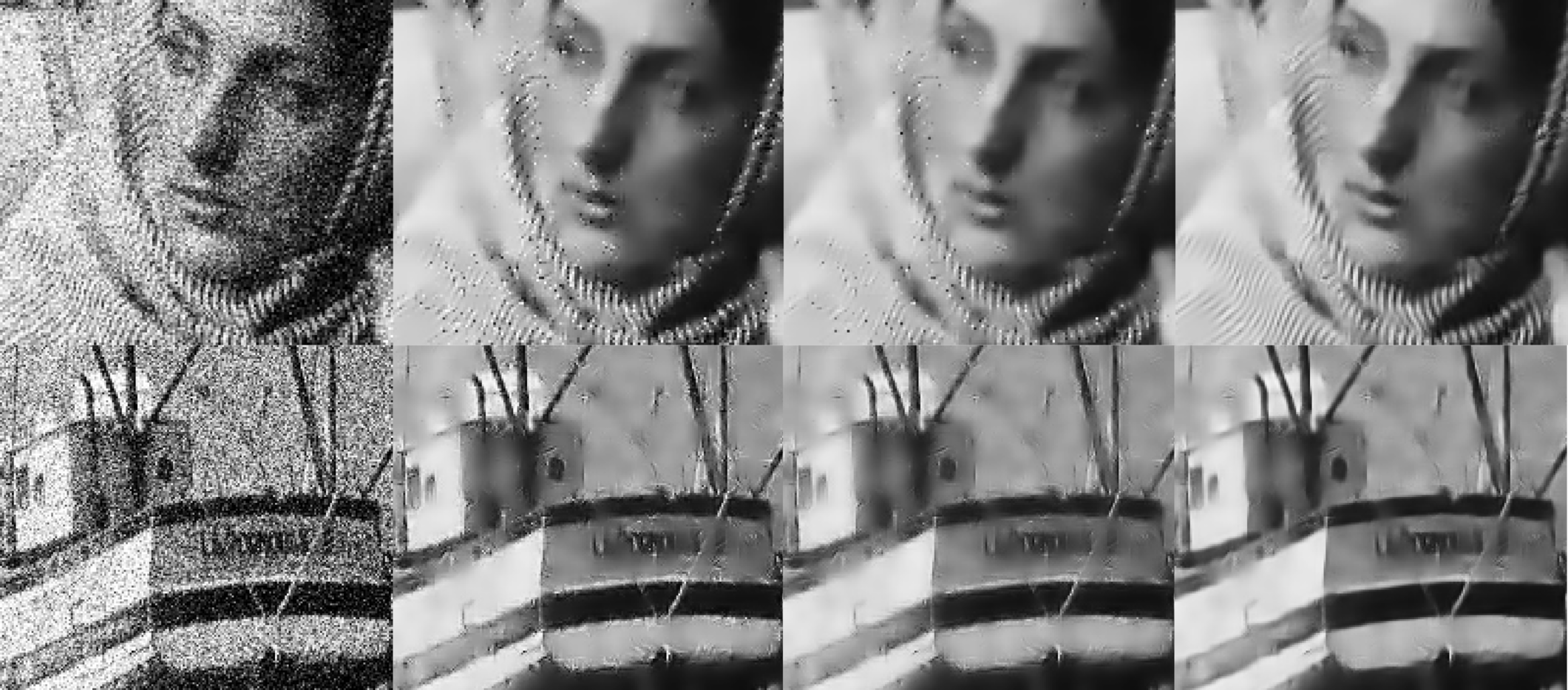
learning moe [1] coding moe barbara 30.4/34.4 31.2/33.8 30.5/34.4 30.9/34.4 34.4 boat 30.4/33.7 30.9/33.4 30.5/33.7 30.8/33.8 33.7 lena 31.8/35.5 32.4/35.1 32.1/35.6 32.3/35.6 35.5 peppers 31.6/34.8 32.1/34.6 31.8/34.9 32.0/34.9 34.8 man 29.6/33.0 30.6/32.9 29.7/33.0 30.2/33.1 32.8 AVERAGE 30.7/34.2 31.4/33.9 30.8/34.2 31.1/34.3 34.1 moe [1] moe 26.5/30.6 26.9/30.2 26.8/30.7 27.0/30.9 30.8 26.9/30.2 27.2/30.1 27.1/30.3 27.3/30.4 30.3 28.3/32.3 28.6/32.0 28.7/32.3 28.8/32.4 32.4 28.3/31.9 28.7/31.8 28.6/31.9 28.7/32.0 31.9 25.8/28.8 26.3/28.9 26.0/28.9 26.2/29.0 28.8 27.0/30.6 27.4/30.4 27.3/30.6 27.5/30.8 30.6 moe [1] moe 24.5/28.2 24.8/28.2 24.8/28.3 24.9/28.5 28.4 25.0/28.1 25.2/28.2 25.3/28.2 25.4/28.3 28.2 26.4/30.1 26.6/30.2 26.7/30.3 26.8/30.4 30.3 26.3/29.8 26.6/29.9 26.6/29.9 26.7/29.9 - 23.9/26.5 24.2/26.8 24.1/26.6 24.2/26.7 26.5 25.1/28.3 25.4/28.5 25.4/28.4 25.5/28.5 28.4
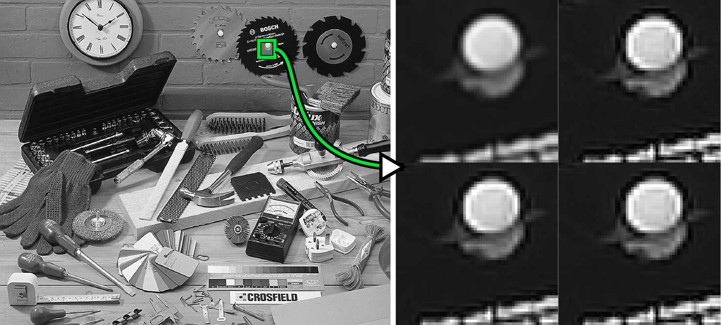
| image | cubic | moe | ||
|---|---|---|---|---|
| barbara | 25.0 | 25.6 | 25.5 | 25.6 |
| boat | 28.9 | 29.8 | 29.8 | 29.9 |
| lena | 32.7 | 33.8 | 33.8 | 33.9 |
| peppers | 32.0 | 33.4 | 33.4 | 33.4 |
| man | 28.4 | 29.4 | 29.3 | 29.4 |
| tools | 21.0 | 22.3 | 22.2 | 22.3 |
| AVER | 22.8 | 24.0 | 24.0 | 24.1 |
V-E Zooming
As an example of signal recovery in the absence of noise, we took the previous set of images, plus a particularly challenging one (Tools), and subsampled them to half each side. We then simulated a zooming effect by upsampling them and estimating each of the 75% missing pixels (see e.g., [50] and references therein). We use a technique similar to the one used in [32]. The image is first interpolated and then deconvoluted using a Wiener filter. The deconvoluted image has artifacts that we treat as noise in the reconstruction. However, since there is no real noise, we do not perform averaging of the patches, using only the center pixel of to fill in the missing pixel at . The results are summarized in Figure 5, where we again observe that using moe instead of and improves the results.
V-F Classification with universal sparse models
In this section we apply our proposed universal models to a classification problem where each sample is to be assigned a class label , which serves as an index to the set of possible classes, . We follow the procedure of [36], where the classifier assigns each sample by means of the maximum a posteriori criterion (5) with the term corresponding to the assumed prior, and the dictionaries representing each class are learned from training samples using (21) with the corresponding regularizer . Each experiment is repeated for the baseline Laplacian model, implied in the regularizer, and the universal model moe, and the results are then compared. In this case we expect that the more accurate prior model for the coefficients will result in an improved likelihood estimation, which in turn should improve the accuracy of the system.
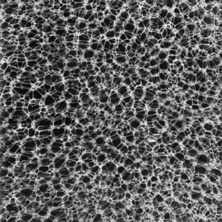
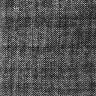
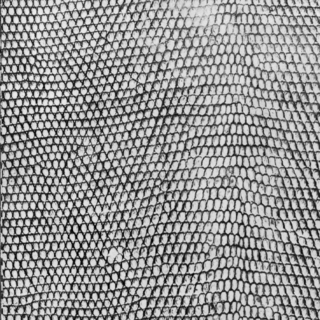
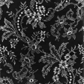
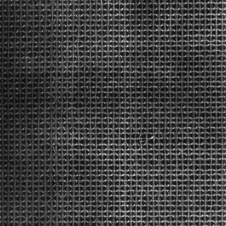
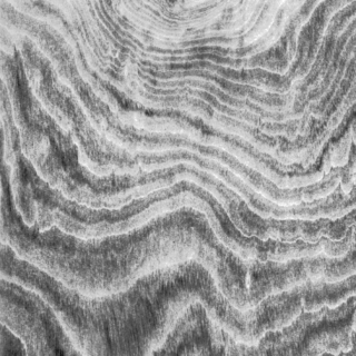
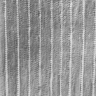
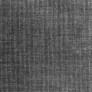
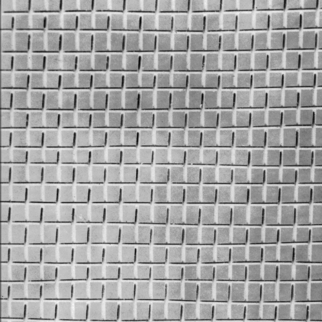
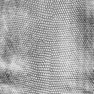
We begin with a classic texture classification problem, where patches have to be identified as belonging to one out of a number of possible textures. In this case we experimented with samples of and textures drawn at random from the Brodatz database,111111http://www.ux.uis.no/~tranden/brodatz.html, the ones actually used shown in Figure 6. In each case the experiment was repeated times. In each repetition, a dictionary of atoms was learned from all patches of the leftmost halves of each sample texture. We then classified the patches from the rightmost halves of the texture samples. For the we obtained an average error rate of using against when using moe, which represents a reduction of in classification error. For the average error rate obtained was using and using moe, which is lower. Thus, using the universal model instead of yields a significant improvement in this case (see for example [26] for other results in classification of Brodatz textures).

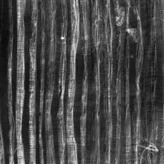
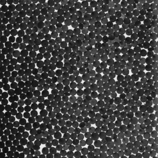
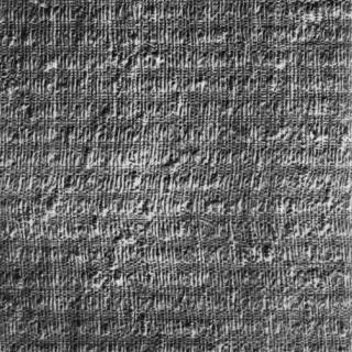
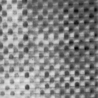
The second sample problem presented is the Graz’02 bike detection problem,121212http://lear.inrialpes.fr/people/marszalek/data/ig02/ where each pixel of each testing image has to be classified as either background or as part of a bike. In the Graz’02 dataset, each of the pixels can belong to one of two classes: bike or background. On each of the training images (which by convention are the first 150 even-numbered images), we are given a mask that tells us whether each pixel belongs to a bike or to the background. We then train a dictionary for bike patches and another for background patches. Patches that contain pixels from both classes are assigned to the class corresponding to the majority of their pixels.
In Figure 7 we show the precision vs. recall curves obtained with the detection framework when either the or the moe regularizers were used in the system. As can be seen, the moe-based model outperforms the in this classification task as well, giving a better precision for all recall values.
In the above experiments, the parameters for the prior (), the moe model () and the incoherence term () were all adjusted by cross validation. The only exception is the moe parameter , which was chosen based on the fitting experiment as .

VI Concluding remarks
A framework for designing sparse modeling priors was introduced in this work, using tools from universal coding, which formalizes sparse coding and modeling from a MDL perspective. The priors obtained lead to models with both theoretical and practical advantages over the traditional and -based ones. In all derived cases, the designed non-convex problems are suitable to be efficiently (approximately) solved via a few iterations of (weighted) subproblems. We also showed that these priors are able to fit the empirical distribution of sparse codes of image patches significantly better than the traditional iid Laplacian model, and even the non-identically distributed independent Laplacian model where a different Laplacian parameter is adjusted to the coefficients associated to each atom, thus showing the flexibility and accuracy of these proposed models. The additional flexibility, furthermore, comes at a small cost of only parameters that can be easily and efficiently tuned (either in the moe model, or in the joe model), instead of (dictionary size), as in weighted models. The additional accuracy of the proposed models was shown to have significant practical impact in active set recovery of sparse signals, image denoising, and classification applications. Compared to the Bayesian approach, we avoid the potential burden of solving several sampled sparse problems, or being forced to use a conjugate prior for computational reasons (although in our case, a fortiori, the conjugate prior does provide us with a good model). Overall, as demonstrated in this paper, the introduction of information theory tools can lead to formally addressing critical aspects of sparse modeling.
Future work in this direction includes the design of priors that take into account the nonzero mass at that appears in overcomplete models, and online learning of the model parameters from noisy data, following for example the technique in [30].
Acknowledgments
Work partially supported by nga, onr, aro, nsf, nsseff, and fundaciba-antel. We wish to thank Julien Mairal for providing us with his fast sparse modeling toolbox, SPAMS.131313http://www.di.ens.fr/willow/SPAMS/ We also thank Federico Lecumberry for his participation on the incoherent dictionary learning method, and helpful comments.
Derivation of the MOE model
In this case we have and which, when plugged into (9), gives
After the change of variables (, ), the integral can be written as
obtaining since the integral on the second line is precisely the definition of . The symmetrization is obtained by substituting by and dividing the normalization constant by two,
The mean of the moe distribution (which is defined only for ) can be easily computed using integration by parts,
In the same way, it is easy to see that the non-central moments of order are
The mle estimates of and can be obtained using any nonlinear optimization technique such as Newton method, using for example the estimates obtained with the method of moments as a starting point. In practice, however, we have not observed any significant improvement in using the mle estimates over the moments-based ones.
Expected approximation error in cost function
As mentioned in the optimization section, the LLA approximates the moe regularizer as a weighted . Here we develop an expression for the expected error between the true function and the approximate convex one, where the expectation is taken (naturally) with respect to the moe distribution. Given the value of the current iterate , (assumed positive, since the function and its approximation are symmetric), the approximated regularizer is . We have
Derivation of the constrained Jeffreys (JOE) model
In the case of the exponential distribution, the Fisher Information Matrix in (15) evaluates to
By plugging this result into (14) with , we obtain We now derive the (one-sided) joe probability density function by plugging this in (9),
Although cannot be evaluated at , the limit for exists and is finite, so we can just define as this limit, which is
Again, if desired, parameter estimation can be done for example using maximum likelihood (via nonlinear optimization), or using the method of moments. However, in this case, the method of moments does not provide a closed form solution for . The non-central moments of order are
| (22) |
For , both integrals in (22) are trivially evaluated, yielding . For , these integrals can be solved using integration by parts:
where the first term in the right hand side of both equations evaluates to for . Therefore, for we obtain the recursions which, combined with the result for , give the final expression for all the moments of order
In particular, for and we have which, when combined, give us
| (23) |
One possibility is to solve the nonlinear equation for by finding the roots of the nonlinear equation and choosing one of them based on some side information. Another possibility is to simply fix the ratio beforehand and solve for and using (23).
Derivation of the conditional Jeffreys (CMOE) model
The conditional Jeffreys method defines a proper prior by assuming that samples from the data to be modeled were already observed. Plugging the Fisher information for the exponential distribution, , into (18) we obtain
Denoting and performing the change of variables we obtain
where the last equation derives from the definition of the Gamma function, . We see that the resulting prior is a Gamma distribution Gamma with and .
References
- [1] M. Aharon, M. Elad, and A. Bruckstein. The K-SVD: An algorithm for designing of overcomplete dictionaries for sparse representations. IEEE Trans. SP, 54(11):4311–4322, Nov. 2006.
- [2] A. Barron, J. Rissanen, and B. Yu. The minimum description length principle in coding and modeling. IEEE Trans. IT, 44(6):2743–2760, 1998.
- [3] J. Bernardo and A. Smith. Bayesian Theory. Wiley, 1994.
- [4] A. Bruckstein, D. Donoho, and M. Elad. From sparse solutions of systems of equations to sparse modeling of signals and images. SIAM Review, 51(1):34–81, Feb. 2009.
- [5] E. J. Candès. Compressive sampling. Proc. of the International Congress of Mathematicians, 3, Aug. 2006.
- [6] E. J. Candès, M. Wakin, and S. Boyd. Enhancing sparsity by reweighted minimization. J. Fourier Anal. Appl., 14(5):877–905, Dec. 2008.
- [7] R. Chartrand. Fast algorithms for nonconvex compressive sensing: MRI reconstruction from very few data. In IEEE ISBI, June 2009.
- [8] S. Chen, D. Donoho, and M. Saunders. Atomic decomposition by basis pursuit. SIAM Journal on Scientific Computing, 20(1):33–61, 1998.
- [9] R. Coifman and M. Wickenhauser. Entropy-based algorithms for best basis selection. IEEE Trans. IT, 38:713–718, 1992.
- [10] T. Cover and J. Thomas. Elements of information theory. John Wiley and Sons, Inc., 2 edition, 2006.
- [11] I. Daubechies, M. Defrise, and C. De Mol. An iterative thresholding algorithm for linear inverse problems with a sparsity constraint. Comm. on Pure and Applied Mathematics, 57:1413–1457, 2004.
- [12] B. Efron, T. Hastie, I. Johnstone, and R. Tibshirani. Least angle regression. Annals of Statistics, 32(2):407–499, 2004.
- [13] M. Elad. Optimized projections for compressed-sensing. IEEE Trans. SP, 55(12):5695–5702, Dec. 2007.
- [14] K. Engan, S. Aase, and J. Husoy. Multi-frame compression: Theory and design. Signal Processing, 80(10):2121–2140, Oct. 2000.
- [15] M. Everingham, A. Zisserman, C. Williams, and L. Van Gool. The PASCAL Visual Object Classes Challenge 2006 (VOC2006) Results. http://www.pascal-network.org/challenges/VOC/voc2006/results.pdf.
- [16] J. Fan and R. Li. Variable selection via nonconcave penalized likelihood and its oracle properties. Journal Am. Stat. Assoc., 96(456):1348–1360, Dec. 2001.
- [17] M. Figueiredo. Adaptive sparseness using Jeffreys prior. In Thomas G. Dietterich, Suzanna Becker, and Zoubin Ghahramani, editors, Adv. NIPS, pages 697–704. MIT Press, Dec. 2001.
- [18] S. Foucart and M. Lai. Sparsest solutions of underdetermined linear systems via -minimization for . Applied and Computational Harmonic Analysis, 3(26):395–407, 2009.
- [19] G. Gasso, A. Rakotomamonjy, and S. Canu. Recovering sparse signals with non-convex penalties and DC programming. IEEE Trans. SP, 57(12):4686–4698, 2009.
- [20] R. Giryes, Y. Eldar, and M. Elad. Automatic parameter setting for iterative shrinkage methods. In IEEE 25-th Convention of Electronics and Electrical Engineers in Israel (IEEEI’08), Dec. 2008.
- [21] P. Grünwald. The Minimum Description Length Principle. MIT Press, June 2007.
- [22] T. Hastie, R. Tibshirani, and J. Friedman. The Elements of Statistical Learning: Data Mining, Inference and Prediction. Springer, 2 edition, Feb. 2009.
- [23] S. Ji, Y. Xue, and L. Carin. Bayesian compressive sensing. IEEE Trans. SP, 56(6):2346–2356, 2008.
- [24] B. Krishnapuram, L. Carin, M. Figueiredo, and A. Hartemink. Sparse multinomial logistic regression: Fast algorithms and generalization bounds. IEEE Trans. PAMI, 27(6):957–968, 2005.
- [25] E. Lam and J. Goodman. A mathematical analysis of the DCT coefficient distributions for images. IEEE Trans. IP, 9(10):1661–1666, 2000.
- [26] J. Mairal, F. Bach, J. Ponce, G. Sapiro, and A. Zisserman. Supervised dictionary learning. In D. Koller, D. Schuurmans, Y. Bengio, and L. Bottou, editors, Adv. NIPS, volume 21, Dec. 2009.
- [27] J. Mairal, G. Sapiro, and M. Elad. Learning multiscale sparse representations for image and video restoration. SIAM MMS, 7(1):214–241, April 2008.
- [28] S. Mallat and Z. Zhang. Matching pursuit in a time-frequency dictionary. IEEE Trans. SP, 41(12):3397–3415, 1993.
- [29] N. Merhav and M. Feder. Universal prediction. IEEE Trans. IT, 44(6):2124–2147, Oct. 1998.
- [30] G. Motta, E. Ordentlich, I. Ramirez, G. Seroussi, and M. Weinberger. The DUDE framework for grayscale image denoising. Technical report, HP laboratories, 2009. http://www.hpl.hp.com/techreports/2009/HPL-2009-252.html.
- [31] P. Moulin and J. Liu. Analysis of multiresolution image denoising schemes using generalized-Gaussian and complexity priors. IEEE Trans. IT, April 1999.
- [32] R. Neelamani, H. Choi, and R. Baraniuk. Forward: Fourier-wavelet regularized deconvolution for ill-conditioned systems. IEEE Trans. SP, 52(2):418–433, 2004.
- [33] B. Olshausen and D. Field. Sparse coding with an overcomplete basis set: A strategy employed by V1? Vision Research, 37:3311–3325, 1997.
- [34] R. Raina, A. Battle, H. Lee, B. Packer, and A. Ng. Self-taught learning: transfer learning from unlabeled data. In ICML, pages 759–766, June 2007.
- [35] I. Ramirez, F. Lecumberry, and G. Sapiro. Universal priors for sparse modeling. In CAMSAP, Dec. 2009.
- [36] I. Ramírez, P. Sprechmann, and G. Sapiro. Classification and clustering via dictionary learning with structured incoherence and shared features. In CVPR, June 2010.
- [37] J. Rissanen. Universal coding, information, prediction and estimation. IEEE Trans. IT, 30(4), July 1984.
- [38] J. Rissanen. Stochastic complexity in statistical inquiry. Singapore: World Scientific, 1992.
- [39] R. Saab, R. Chartrand, and O. Yilmaz. Stable sparse approximation via nonconvex optimization. In ICASSP, April 2008.
- [40] N. Saito. Simultaneous noise suppression and signal compression using a library of orthonormal bases and the MDL criterion. In E. Foufoula-Georgiou and P. Kumar, editors, Wavelets in Geophysics, pages 299––324. New York: Academic, 1994.
- [41] G. Schwartz. Estimating the dimension of a model. Annals of Statistics, 6(2):461–464, 1978.
- [42] Y. Shtarkov. Universal sequential coding of single messages. Probl. Inform. Transm., 23(3):3–17, July 1987.
- [43] R. Tibshirani. Regression shrinkage and selection via the LASSO. Journal of the Royal Statistical Society: Series B, 58(1):267–288, 1996.
- [44] M. Tipping. Sparse bayesian learning and the relevance vector machine. Journal of Machine Learning, 1:211–244, 2001.
- [45] J. Tropp. Greed is good: Algorithmic results for sparse approximation. IEEE Trans. IT, 50(10):2231–2242, Oct. 2004.
- [46] J. Trzasko and A. Manduca. Highly undersampled magnetic resonance image reconstruction via homotopic -minimization. IEEE Trans. MI, 28(1):106–121, Jan. 2009.
- [47] J. Trzasko and A. Manduca. Relaxed conditions for sparse signal recovery with general concave priors. IEEE Trans. SP, 57(11):4347–4354, 2009.
- [48] D. Wipf, J. Palmer, and B. Rao. Perspectives on sparse bayesian learning. In Adv. NIPS, Dec. 2003.
- [49] D. Wipf and B. Rao. An empirical bayesian strategy for solving the simultaneous sparse approximation problem. IEEE Trans. IP, 55(7-2):3704–3716, 2007.
- [50] G. Yu, G. Sapiro, and S. Mallat. Solving inverse problems with piecewise linear estimators: From Gaussian mixture models to structured sparsity. Preprint arXiv:1006.3056.
- [51] H. Zou. The adaptive LASSO and its oracle properties. Journal Am. Stat. Assoc., 101:1418–1429, 2006.
- [52] H. Zou and R. Li. One-step sparse estimates in nonconcave penalized likelihood models. Annals of Statistics, 36(4):1509–1533, 2008.