Self-Calibration of Radio Astronomical Arrays With Non-Diagonal Noise Covariance Matrix

Abstract

The radio astronomy community is currently building a number of phased array telescopes. The calibration of these telescopes is hampered by the fact that covariances of signals from closely spaced antennas are sensitive to noise coupling and to variations in sky brightness on large spatial scales. These effects are difficult and computationally expensive to model. We propose to model them phenomenologically using a non-diagonal noise covariance matrix. The parameters can be estimated using a weighted alternating least squares (WALS) algorithm iterating between the calibration parameters and the additive nuisance parameters. We demonstrate the effectiveness of our method using data from the low frequency array (LOFAR) prototype station.

1 Introduction

The radio astronomical community is currently constructing a number of large scale phased array telescopes such as the low-frequency array (LOFAR) [1] and the Murchison wide field array (MWA) [2]. These instruments need to be calibrated regularly to track variations in the electronics of the antennas and receivers, as well as direction dependent variations of the ionosphere [3]. E.g., LOFAR will consist of order 50 stations (distributed over an area of a hundred kilometers or more), where each station consists of 96 “low band” dual-polarized dipole antennas (10–90 MHz) and 96 “high band” antennas (110–240 MHz). The latter antennas are in turn composed of 16 beamformed dual-polarized droopy dipole antennas. Each station provides a number of beamformed outputs, which in turn are correlated at a central location to form images and other astronomy products.

In this paper we focus on the calibration of the station antennas. The general aim is to estimate the direction independent gains and phases of each sensor, as well as the direction dependent gains corresponding to each source. This is done for the 2–10 brightest sources in the sky, assuming a point source model. The problem is complicated by the fact that the covariances of signals from closely spaced antennas within a station are sensitive to noise coupling (for the lowest frequencies, the antennas are spaced closer than half a wavelength). Also, the point source model does not entirely hold because of bright emission from the plane of the galaxy, extending over the entire sky. Fortunately, this emission is spatially smooth, which implies that it is dominant on the short spatial scales in the array aperture, i.e. on the short baselines. In this paper we propose to model both short baseline effects by an additive noise covariance matrix, which in this case is not diagonal and has unknown entries for each short baseline. If we can estimate this matrix, a simple point source model will be sufficient to calibrate the array, which reduces the problem to a problem for which solutions are readily available [4, 5, 6].

Direction finding problems for calibrated arrays in the presence of unknown correlated noise have been extensively studied in the 1990s. It was proven that the general problem is not tractable without imposing some appropriate constraints on the noise covariance matrix or exploiting differences in temporal characteristics between source and noise signals [7]. Radio astronomical signals generally behave like noise, thus temporal techniques (instrumental variables) are not applicable. Instead, we should rely on an appropriately constrained parameterized model of the noise covariance matrix. Starting with [8], a series of papers were published; see [9] for an overview. ML estimators for the source and instrument parameters under a generalized noise covariance parameterization is provided in [10, 9], whereas nonlinear least squares estimators were studied in [10, 11, 12]. In either case, an analytic source and instrument parameter dependent solution is derived for the noise model parameters which is substituted back into the cost function. This cost function then has to be minimized using a generalized solving technique, such as Newton iterations. This approach works well if the number of instrument and source parameters is small. For larger problems (we consider 100 antenna/source parameters and over 750 noise covariance parameters), it is convenient to exploit suboptimal but closed-form analytic solutions, at least for initialization. We therefore propose a weighted alternating least squares (WALS) approach which iterates over noise, source and instrument parameters. The proposed method can thus be regarded as an extension to the methods proposed in [6]

Notation: The transpose operator is denoted by ^T, the complex conjugate (Hermitian) transpose by ^H, complex conjugation by $\overline{(\cdot)}$ and the pseudo-inverse by ^†. An estimated value is denoted by $\widehat{(\cdot)}$. $\otimes$ denotes the Kronecker product and $\circ$ is used to denote the Khatri-Rao or column-wise Kronecker product of two matrices. $\mathrm{vec}(\cdot)$ converts a matrix to a vector by stacking the columns of the matrix.

2 Data Model and problem statement

We consider an array of $P$ antennas. The measured $P\times P$ array covariance matrix can be modeled as

$$\mathbf{R}=\mathbf{R}_{0}\left(\mbox{\boldmath{$\theta$}}\right)+\mbox{\boldmath{$\Sigma$}}_{n}$$ (1)

where $\mathbf{R}_{0}\left(\mbox{\boldmath{$\theta$}}\right)$ is the signal model for an ideal noise free array, which depends on a number of unknown real valued parameters accumulated in a column vector $\theta$, and $\mbox{\boldmath{$\Sigma$}}_{n}$ is a $P\times P$ matrix describing the noise corruption. Note that $\mbox{\boldmath{$\Sigma$}}_{n}$ must be Hermitian, since the array covariance matrix is a Hermitian matrix. In our application, the data covariance model is

$$\mathbf{R}_{0}\left(\mbox{\boldmath{$\theta$}}\right)=\mathbf{G}_{1}\mathbf{A}\mathbf{G}_{2}\mbox{\boldmath{$\Sigma$}}_{s}\mathbf{G}_{2}^{H}\mathbf{A}^{H}\mathbf{G}_{1}^{H}$$ (2)

where $\mbox{\boldmath{$\Sigma$}}_{s}$ is the covariance of the point sources (assumed to be known from tables), $\mathbf{A}$ contains the direction vectors, $\mathbf{G}_{1}$ a (diagonal) instrumental gain/phase matrix, and $\mathbf{G}_{2}$ a (diagonal) direction dependent gain matrix [6]. If the direction dependent gains are unknown, we can introduce $\mbox{\boldmath{$\Sigma$}}=\mathbf{G}_{2}\mbox{\boldmath{$\Sigma$}}_{s}\mathbf{G}_{2}^{H}$, which implies that we should estimate the apparent source powers. The direction dependent gains follow directly from the apparent source powers if the actual source powers are known, e.g. from tables. If the source positions are unknown or perturbed by propagation conditions, $\mathbf{A}$ may be parameterized [6]. The contents of the parameter vector $\theta$ therefore strongly depend on the available knowledge on the instrument, the propagation conditions and the sources.

As in [8] and subsequent papers, the unknown noise covariance matrix is modeled as a linear sum of known matrices, in this case simple selection matrices $\mathbf{E}_{ij}$ which are zero everywhere except for a ’1’ in entry $(i,j)$,

$$\mbox{\boldmath{$\Sigma$}}_{n}=\sum_{(i,j)\in\cal{S}}\sigma_{ij}\mathbf{E}_{ij}\,.$$

The set $\cal{S}$ contains the index pairs of the short baselines, including the autocorrelation entries $(i,i)$. The unknown coefficients $\sigma_{ij}$ are the nuisance parameters.

In the absence of the noise corruptions, i.e., $\mathbf{R}=\mathbf{R}_{0}\left(\mbox{\boldmath{$\theta$}}\right)$, the estimation problem to find the parameter vector $\theta$ is commonly formulated either as a ML problem, or as a generalized least squares estimation problem

$$\widehat{\mbox{\boldmath{$\theta$}}}=\underset{\mbox{\boldmath{$\theta$}}}{\mathrm{argmin}}\left\Arrowvert\mathbf{W}\left(\widehat{\mathbf{R}}-\mathbf{R}_{0}\left(\mbox{\boldmath{$\theta$}}\right)\right)\mathbf{W}\right\Arrowvert_{F}^{2},$$ (3)

where $\widehat{\mathbf{R}}$ is the measured array covariance matrix. It is known that with $\mathbf{W}=\mathbf{R}^{-1/2}$ this estimator is asymptotically unbiased and asymptotically efficient [10, 12]. Indeed, the simulations in [10] show only a small improvement of the ML solution as compared to the WLS solution. For $\mathbf{R}_{0}(\mbox{\boldmath{$\theta$}})$ given in (2), this problem, as well as the case with an unknown diagonal noise covariance, was studied by us in [6], in the present paper, we will assume that a solution to this problem is available.

In the presence of correlated noise on the short baselines, the problem is extended to

$$\left\{\widehat{\mbox{\boldmath{$\theta$}}},\widehat{\mbox{\boldmath{$\sigma$}}}_{n}\right\}=\underset{\mbox{\boldmath{$\theta$}},\mbox{\boldmath{$\sigma$}}_{n}}{\mathrm{argmin}}\left\Arrowvert\mathbf{W}\left(\widehat{\mathbf{R}}-\mathbf{R}_{0}\left(\mbox{\boldmath{$\theta$}}\right)-\mbox{\boldmath{$\Sigma$}}_{n}\right)\mathbf{W}\right\Arrowvert_{F}^{2},$$ (4)

where $\mbox{\boldmath{$\sigma$}}_{n}$ is a vector containing all unique real valued parameters required to describe the nonzero entries of $\mbox{\boldmath{$\Sigma$}}_{n}$. This vector can be related to $\mbox{\boldmath{$\Sigma$}}_{n}$ using a selection matrix $\mathbf{I}_{s}$ such that $\mathrm{vec}\left(\mbox{\boldmath{$\Sigma$}}_{n}\right)=\mathbf{I}_{s}\mbox{\boldmath{$\sigma$}}_{n}$. By choosing the selection matrix appropriately, we can ensure that the estimated $\mbox{\boldmath{$\Sigma$}}_{n}$ is Hermitian.

3 Parameter estimation

3.1 Weighted Alternating Least Squares

We propose to solve the problem in Eq. (4) by alternating between weighted least squares (WLS) estimation of the desired parameters $\theta$ and WLS estimation of the nuisance parameters $\mbox{\boldmath{$\sigma$}}_{n}$. The first WLS problem can be formulated as

$$\widehat{\mbox{\boldmath{$\theta$}}}=\underset{\mbox{\boldmath{$\theta$}}}{\mathrm{argmin}}\left\Arrowvert\mathbf{W}\left(\left(\widehat{\mathbf{R}}-\mbox{\boldmath{$\Sigma$}}_{n}\right)-\mathbf{R}_{0}\left(\mbox{\boldmath{$\theta$}}\right)\right)\mathbf{W}\right\Arrowvert_{F}^{2}.$$ (5)

which is identical in form to Eq. (3) for which a solution is assumed to be available.

The second WLS problem can be formulated as

$$\widehat{\mbox{\boldmath{$\sigma$}}}_{n} = \underset{\mbox{\boldmath{$\sigma$}}_{n}}{\mathrm{argmin}}\left\Arrowvert\mathbf{W}\left(\left(\widehat{\mathbf{R}}-\mathbf{R}_{0}\left(\mbox{\boldmath{$\theta$}}\right)\right)-\mbox{\boldmath{$\Sigma$}}_{n}\right)\mathbf{W}\right\Arrowvert_{F}^{2}$$ (6)

$$= \underset{\mbox{\boldmath{$\sigma$}}_{n}}{\mathrm{argmin}}\Big{\Arrowvert}\left(\overline{\mathbf{W}}\otimes\mathbf{W}\right)\mathrm{vec}\left(\widehat{\mathbf{R}}-\mathbf{R}_{0}\left(\mbox{\boldmath{$\theta$}}\right)\right)-$$

$$\left(\overline{\mathbf{W}}\otimes\mathbf{W}\right)\mathbf{I}_{s}\mbox{\boldmath{$\sigma$}}_{n}\Big{\Arrowvert}_{F}^{2}.$$

The solution to this problem is given by

$$\widehat{\mbox{\boldmath{$\sigma$}}}_{n}=\left(\left(\overline{\mathbf{W}}\otimes\mathbf{W}\right)\mathbf{I}_{s}\right)^{\dagger}\left(\overline{\mathbf{W}}\otimes\mathbf{W}\right)\mathrm{vec}\left(\widehat{\mathbf{R}}-\mathbf{R}_{0}\left(\mbox{\boldmath{$\theta$}}\right)\right).$$ (7)

In section 2 it was mentioned that $\mathbf{W}=\mathbf{R}^{-1/2}$ provides optimal weighting for the LS cost function. Since $\mathbf{R}$ is not known, $\widehat{\mathbf{R}}$ is used instead in many applications. It can be shown that this may lead to a bias in the estimate of $\widehat{\mbox{\boldmath{$\sigma$}}}_{n}$ for a finite number of samples [6]. This bias can be avoided by using the best available model $\mathbf{R}\left(\widehat{\mbox{\boldmath{$\theta$}}},\widehat{\mbox{\boldmath{$\sigma$}}}_{n}\right)$ instead of $\widehat{\mathbf{R}}$.

Estimation of receiver noise powers is a special case of the general problem treated here. In this case $\mbox{\boldmath{$\Sigma$}}_{n}$ is a diagonal, and $\mathbf{I}_{s}=\mathbf{I}\circ\mathbf{I}$ where $\mathbf{I}$ is the $P\times P$ identity matrix. This form of selection matrix simplifies Eq. (7) considerably [6]. In some problems, for example in estimating the receiver based gains, it is then possible to simply ignore the diagonal entries instead of including nuisance parameters [5]. It can further be shown that ignoring the corrupted entries instead of including them using nuisance parameters does not change the Cramèr-Rao bound of the parameters of interest [13]. This can be explained intuitively by regarding the matrix equation describing the WLS problem as a set of scalar equations. If a unique nuisance parameter is added to one of those scalar equations, that equation is required to solve for the nuisance parameter and can thus not be used to solve any other parameters. This implies that this equation could have been ignored if one would only focus on the parameters of interest. In practice, however, it may be hard to develop an algorithm that ignores the corrupted entries in a statistically efficient way.

3.2 Algorithm

The resulting algorithm is as follows:

1. Initialization Set the iteration counter $i=1$ and initialize $\widehat{\mbox{\boldmath{$\sigma$}}}_{n}^{[0]}$ based on any prior information if available, otherwise initialize $\widehat{\mbox{\boldmath{$\sigma$}}}_{n}^{[0]}$ to zero. Initially use $\mathbf{W}=\widehat{\mathbf{R}}^{-1/2}$.

2. Estimate $\widehat{\mbox{\boldmath{$\theta$}}}^{[i]}$ by solving the WLS problem formulated in Eq. (5) using $\widehat{\mbox{\boldmath{$\sigma$}}}_{n}^{[i-1]}$ as prior knowledge.

3. Estimate $\widehat{\mbox{\boldmath{$\sigma$}}}_{n}^{[i]}$ using Eq. (7) using $\widehat{\mbox{\boldmath{$\theta$}}}^{[i]}$ as prior knowledge.

4. Update $\mathbf{W}=\mathbf{R}^{-1/2}$ to avoid the bias mentioned in the previous section.

5. Check for convergence, otherwise continue with step 2.

An algorithm that alternatingly optimizes for distinct groups of parameters, in our case $\theta$ and $\mbox{\boldmath{$\sigma$}}_{n}$, can be proven to converge if the value of the cost function decreases in each iteration. We assume that a suitable method is available to find $\theta$. Since we propose to estimate $\mbox{\boldmath{$\sigma$}}_{n}$ using the well known standard solution for least squares estimation problems, the value of the cost function will decrease in both steps, thus ensuring convergence. Although there is no guarantee that the algorithm will converge to the global optimum, practical experience with LOFAR and results from Monte Carlo simulations in this paper and in earlier papers [5, 6] indicate that the proposed method produces good results for most reasonable initial estimates.

4 Experimental results

4.1 The LOFAR prototype station

Figure 1: Array configuration of the 48 antenna LOFAR prototype station.

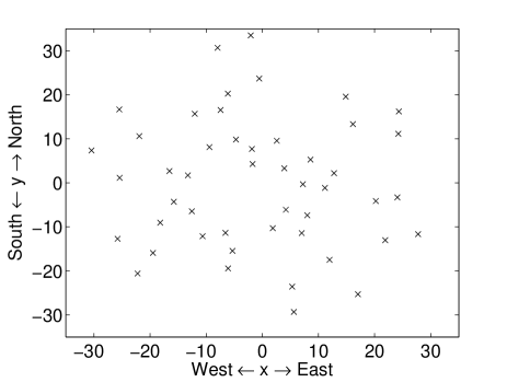
The first full-scale LOFAR prototype station with real-time backend became operational in the second quarter of 2006 [14]. This station consisted of 48 dual-polarization antennas operating between 10 and 90 MHz arranged in a randomized configuration based on rings with exponentially increasing radii as shown in Fig. 1. Each of the two signals from every antenna was filtered and digitized using a 12-bit 200 MHz ADC. A real-time FPGA based digital processing backend splits the 100 MHz Nyquist sampled base band in 512 subbands, each 195 kHz wide, using a polyphase filter. The backend also provides a correlator which can correlate in real-time the data from the 96 input channels for a single subband. This subband may be any of the 512 available subbands and this choice may change every second.

4.2 Results

For the demonstration in this paper we used data from a single 1 s snapshot observation in the 195 kHz subband centered at 50 MHz. This observation was done on 14 February 2008 at 1:42:07 UTC. We will calibrate the data using the method described in Sec. 3.2, where we will model correlated noise terms on all baselines shorter than four wavelengths. The complete WLS problem thus implies estimation of the amplitudes (48 parameters) and phases (47 parameters) of the antenna based complex gains, the source power ratio of the two brightest sources (1 parameter) and 764 real valued nuisance parameters describing all non-zero entries of the noise covariance matrix for a total of 860 free real valued parameters per polarization. In this experiment we show that use of such nuisance parameters can reduce the complex source structure on the sky to a simple model with just two point sources.

Figure 2: Calibrated all-sky map for a single polarization at 50 MHz from the 48-element LOFAR prototype station. The image shows the sky projected on the horizon plane of the station.

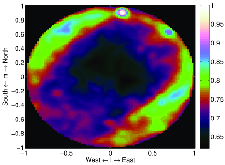
Figure 2 shows a calibrated all sky map for a single polarization. There are two bright point sources near the northeastern horizon. The image also shows a lot of extended emission from the galactic plane (on the northwestern horizon) and the north polar spur (on the eastern horizon). This extended emission is hard to model accurately, but only affects the short baselines since short distances in the aperture plane of a phased array correspond to low spatial frequencies, which describe the structure on large spatial scales.

Figure 3: Calibrated all-sky map of extended emission observed at baselines shorter than four wavelengths for a single polarization at 50 MHz.

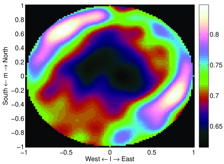
It was found that most of this extended emission is captured by the correlations on baselines shorter than four wavelengths. This affects 358 crosscorrelations and the 48 autocorrelations resulting in the aforementioned 764 real valued parameters to describe the non-zero entries of $\mbox{\boldmath{$\Sigma$}}_{n}$. Using the procedure outlined in the previous section, $\widehat{\mbox{\boldmath{$\sigma$}}}_{n}$ was estimated simultaneously with $\widehat{\mbox{\boldmath{$\theta$}}}$ containing the other parameters. $\widehat{\mbox{\boldmath{$\Sigma$}}}_{n}$ can therefore be interpreted as an estimate of the extended source structure, noise coupling and receiver noise powers. This is nicely demonstrated in Fig. 3 which shows an image based on $\widehat{\mbox{\boldmath{$\Sigma$}}}_{n}$ after the calibration was completed.

Figure 4: Difference between the calibrated all-sky map shown in Fig. 2 and the contribution of extended emission shown in Fig. 3 showing that the remainder can be accurately modeled using a model with just two point sources.

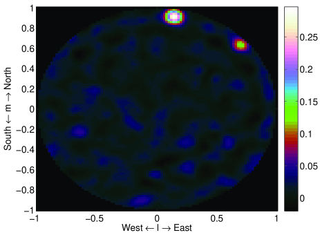
Figure 4 shows the difference between the maps shown in Figs. 2 and 3. This shows that $\mbox{\boldmath{$\Sigma$}}_{n}$ provides a description of the extended emission that is sufficiently accurate to reduce $\widehat{\mathbf{R}}-\widehat{\mbox{\boldmath{$\Sigma$}}}_{n}$ to an array covariance matrix that can be described by a model consisting of only two point sources. This thus reduces our original problem to one that has been discussed extensively in the array signal processing literature.

5 Improving the computational efficiency

The calculation of $\widehat{\mbox{\boldmath{$\sigma$}}}_{n}$ using Eq. 7 forms the most expensive part of the algorithm in terms of CPU and memory usage due to the Kronecker products. These Kronecker products can only be reduced to simpler Khatri-Rao or Hadamard products in a number of special cases, such as a diagonal noise covariance matrix treated in [6]. However, the parameterization of $\mbox{\boldmath{$\Sigma$}}_{n}$ chosen here implies that each entry of the array covariance matrix with a contribution from $\mbox{\boldmath{$\Sigma$}}_{n}$ is affected by a unique additive parameter. Intuitively, one would therefore expect that the weighting in Eq. (7) would not make much difference. Omitting this would reduce the CPU and memory requirements considerably, since the Kronecker products and the inverse increase the numerical complexity from $o\left(NP^{2}\right)$ to $o\left(N^{3}+P^{6}\right)$ and the size of the largest matrix from $P^{2}\times N$ to $P^{2}\times P^{2}$, where $N$ is the number of noise parameters stacked in $\mbox{\boldmath{$\sigma$}}_{n}$.

#	$l$	$m$	$\sigma_{q}^{2}$
1	0.24651	-0.71637	1.00000
2	-0.34346	0.76883	0.88051
3	-0.13125	-0.31463	0.79079
4	-0.29941	-0.52339	0.74654
5	0.39290	0.58902	0.69781

Table 1: Source powers and source locations used in the simulations

This idea was therefore tested in Monte Carlo simulations. For these simulations, a five armed array was defined, each arm being an eight-element, one wavelength spaced ULA. The first element of each arm formed an equally spaced circular array with half wavelength spacing between the elements. The source model is presented in Table 1. This source model was generated with a random number generator to verify that the proposed approach works for arbitrary source models.

Figure 5: Comparison of the variance on the direction independent complex gain and the source power estimates obtained in Monte Carlo simulations with weighted LS estimation of $\widehat{\mbox{\boldmath{$\sigma$}}}_{n}$ and unweighted LS estimation of $\widehat{\mbox{\boldmath{$\sigma$}}}_{n}$.

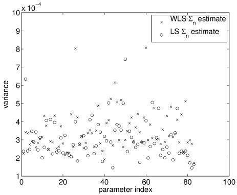
Figure 5 compares the variance on the estimates for the omnidirectional complex gains of the receiving elements and the source powers obtained after 100 runs of a Monte Carlo simulation with weighted LS estimation of $\widehat{\mbox{\boldmath{$\sigma$}}}_{n}$ and the computationally more efficient unweighted LS estimation of $\widehat{\mbox{\boldmath{$\sigma$}}}_{n}$. The complex receiving element gains and the source powers, stacked in $\theta$, were estimated using weighted least squares in both cases. Both algorithms generally converged within three iterations to relative error per parameter of $\sim 10^{-4}$, i.e. well below the Cramèr-Rao bound. The convergence rate in these simulations was one digit per iteration down to the numerical accuracy provided by double precision floating point numbers.

The results indicate that the variance on these estimates is the same in both cases within the accuracy provided by the simulations. We therefore conclude that it is viable to discard the weighting in Eq. (7). With this modification all 860 free parameters in the experiment described in the previous section could be extracted from the actual data using Matlab running on a standard dual core 2.4 GHz CPU in only 0.4 seconds. This implies that a single 2.4 GHz core can keep up with the data from the correlator at the LOFAR station, which real-time correlates the antenna signals for a single subband with one second integration time. This update rate is required to track variations in the electronic gains and the ionosphere.

6 Conclusions

We have demonstrated using data from a LOFAR prototype station that the effects of noise coupling, receiver noise powers and extended emission on a radio astronomical phased array can be phenomenologically described by a non-diagonal noise covariance matrix with non-zero entries on short baselines. These entries can be computationally efficient and accurately estimated by a WALS algorithm alternating between estimation of the correlated noise parameters and calibration parameters.

References

- [1] M. de. Vos, A. W. Gunst and R. Nijboer, “The LOFAR Telescope: System Architecture and Signal Processing,” IEEE Proceedings, 2009, accepted for publication.
- [2] C. Lonsdale, “The Murchison Widefield Array,” in Proceedings of the XXIXth General Assembly of the International Union of Radio Science (URSI GA), Chicago (Ill.), USA, 7-16 Aug. 2008.
- [3] S. van der Tol, B. Jeffs and A. J. van der Veen, “Self Calibration for the LOFAR Radio Astronomical Array,” IEEE Trans. Signal Processing, vol. 55, no. 9, pp. 4497–4510, Sept. 2007.
- [4] D. R. Fuhrmann, “Estimation of Sensor Gain and Phase,” IEEE Trans. Signal Processing, vol. 42, no. 1, pp. 77–87, Jan. 1994.
- [5] S. J. Wijnholds and A. J. Boonstra, “A Multisource Calibration Method for Phased Array Radio Telescopes,” in Fourth IEEE Workshop on Sensor Array and Multi-channel Process ing (SAM), Waltham (MA), 12-14 July 2006.
- [6] S. J. Wijnholds and A. J. van der Veen, “Multisource Self-Calibration for Sensor Arrays,” IEEE Trans. Signal Processing, 2009, in press.
- [7] P. Stoica and T. Söderström, “On Array Signal Processing in Spatially Correlated Noise Fields,” IEEE Trans. Circuits and Systems - II: Analog and Digital Signal Processing, vol. 39, no. 12, pp. 879–882, Dec. 1992.
- [8] J. F. Bohme and D. Kraus, “On Least Squares Methods for Direction of Arrival Estimation in the Presence of Unknown Noise Fields,” in IEEE International Conference on Acoustics, Speech and Signal Processing (ICASSP), 1988, pp. 2833–2836.
- [9] B. Göransson and B. Ottersten, “Direction Estimation in Partially Unknown Noise Fields,” IEEE Trans. Signal Processing, vol. 47, no. 9, pp. 2375–2385, Sept. 1999.
- [10] B. Friedlander and A. J. Weiss, “Direction Finding Using Noise Covariance Modeling,” IEEE Trans. Signal Processing, vol. 43, no. 7, pp. 1557–1567, July 1995.
- [11] M. Wax, J, Sheinvald and A. J. Weiss, “Detection and Localization in Colored Noise via Generalized Least Squares,” IEEE Trans. Signal Processing, vol. 44, no. 7, pp. 1734–1743, July 1996.
- [12] B. Ottersten, P. Stoica and R. Roy, “Covariance Matsching Estimation Techniques for Array Signal Processing Applications,” Digital Signal Processing, A Review Journal, vol. 8, pp. 185–210, July 1998.
- [13] S. van der Tol and S. J. Wijnholds, “CRB Analysis of the Impact of Unknown Receiver Noise on Phased Array Calibration,” in Fourth IEEE Workshop on Sensor Array and Multi-channel Processing (SAM), Waltham (MA), 12-14 July 2006.
- [14] A. W. Gunst and M. J. Bentum, “The Current Design of the LOFAR Instrument,” in Proceedings of the 2007 IEEE International Conference on Signal Processing and Communications (ICSPC 2007), Dubai, United Arab Emirates, 24-27 Nov. 2007.