THE SM AND NLO MULTILEG WORKING GROUP:
Summary Report

Report of the SM and NLO Multileg Working Group for the Workshop “Physics at TeV Colliders”, Les Houches, France, 8–26 June, 2009.

1 INTRODUCTION

After years of waiting, and after six Les Houches workshops, the era of LHC running is finally upon us, albeit at a lower initial center-of-mass energy than originally planned. Thus, there has been a great sense of anticipation from both the experimental and theoretical communities. The last two years, in particular, have seen great productivity in the area of multi-parton calculations at leading order (LO), next-to-leading order (NLO) and next-to-next-to-leading order (NNLO), and this productivity is reflected in the proceedings of the NLM group. Both religions, Feynmanians and Unitarians, as well as agnostic experimenters, were well-represented in both the discussions at Les Houches, and in the contributions to the write-up.

Next-to-leading order (NLO) is the first order at which the normalization, and in some cases the shape, of perturbative cross sections can be considered reliable [1]. This can be especially true when probing extreme kinematic regions, as for example with boosted Higgs searches considered in several of the contributions to this writeup. A full understanding for both standard model and beyond the standard model physics at the LHC requires the development of fast, reliable programs for the calculation of multi-parton final states at NLO. There have been many advances in the development of NLO techniques, standardization and automation for such processes and this is reflected in the contributions to the first section of this writeup.

Many calculations have previously been performed with the aid of semi-numerical techniques. Such techniques, although retaining the desired accuracy, lead to codes which are slow to run. Advances in the calculation of compact analytic expressions for Higgs + 2 jets (see for example the contribution of S. Badger and R. Britto to these proceedings) have resulted in the development of much faster codes, which extend the phenomenology that can be conducted, as well as making the code available to the public for the first time.

A prioritized list of NLO cross sections was assembled at Les Houches in 2005 [2] and added to in 2007 [3]. This list includes cross sections which are experimentally important, and which are theoretically feasible (if difficult) to calculate. Basically all $2\rightarrow 3$ cross sections of interest have been calculated, with the frontier now extending to $2\rightarrow 4$ calculations. Often these calculations exist only as private codes. That wishlist is shown below in Table 1. Since 2007, two additional calculations have been completed: $t\bar{t}b\bar{b}$ and $W$ + 3 jets, reflecting the advance of the NLO technology to $2\rightarrow 4$ processes. In addition, the cross section for $b\bar{b}b\bar{b}$ has been calculated for the $q\bar{q}$ initial state with the $gg$ initial state calculation in progress (see the contribution of T. Binoth et al).

Final states of such complexity usually lead to multi-scale problems, and the correct choice of scales to use can be problematic not only at LO, but also at NLO. The size of the higher order corrections and of the residual scale dependence at NLO can depend strongly on whether the considered cross section is inclusive, or whether a jet veto cut has been applied .

Depending on the process, dramatically different behavior can be observed upon the application of a jet veto. There is a trade-off between suppressing the NLO cross section and increasing the perturbative uncertainty, with application of a jet veto sometimes destroying the cancellation between infra-red logs of real and virtual origin, and sometimes just suppressing large (and very scale-sensitive) tree-level contributions. So far, there is no general rule predicting the type of behavior to be expected, but this is an important matter for further investigation.

Process ($V\in\{Z,W,\gamma\}$)	Comments
Calculations completed since Les Houches 2005
1. $pp\to VV$jet	$WW$jet completed by Dittmaier/Kallweit/Uwer [4, 5];
	Campbell/Ellis/Zanderighi [6].
	$ZZ$jet completed by
	Binoth/Gleisberg/Karg/Kauer/Sanguinetti [7]
2. $pp\to$ Higgs+2jets	NLO QCD to the $gg$ channel
	completed by Campbell/Ellis/Zanderighi [8];
	NLO QCD+EW to the VBF channel
	completed by Ciccolini/Denner/Dittmaier [9, 10]
3. $pp\to V\,V\,V$	$ZZZ$ completed by Lazopoulos/Melnikov/Petriello [11]
	and $WWZ$ by Hankele/Zeppenfeld [12]
	(see also Binoth/Ossola/Papadopoulos/Pittau [13])
4. $pp\to t\bar{t}\,b\bar{b}$	relevant for $t\bar{t}H$ computed by
	Bredenstein/Denner/Dittmaier/Pozzorini [14, 15]
	and Bevilacqua/Czakon/Papadopoulos/Pittau/Worek [16]
5. $pp\to V$+3jets	calculated by the Blackhat/Sherpa [17]
	and Rocket [18] collaborations
Calculations remaining from Les Houches 2005
6. $pp\to t\bar{t}$+2jets	relevant for $t\bar{t}H$ computed by
	Bevilacqua/Czakon/Papadopoulos/Worek  [19]
7. $pp\to VV\,b\bar{b}$,	relevant for VBF $\rightarrow H\rightarrow VV$, $t\bar{t}H$
8. $pp\to VV$+2jets	relevant for VBF $\rightarrow H\rightarrow VV$
	VBF contributions calculated by
	(Bozzi/)Jäger/Oleari/Zeppenfeld [20, 21, 22]
NLO calculations added to list in 2007
9. $pp\to b\bar{b}b\bar{b}$	$q\bar{q}$ channel calculated by Golem collaboration [23]
NLO calculations added to list in 2009
10. $pp\to V$+4 jets	top pair production, various new physics signatures
11. $pp\to Wb\bar{b}j$	top, new physics signatures
12. $pp\to t\bar{t}t\bar{t}$	various new physics signatures
Calculations beyond NLO added in 2007
13. $gg\to W^{*}W^{*}$ ${\cal O}(\alpha^{2}\alpha_{s}^{3})$	backgrounds to Higgs
14. NNLO $pp\to t\bar{t}$	normalization of a benchmark process
15. NNLO to VBF and $Z/\gamma$+jet	Higgs couplings and SM benchmark
Calculations including electroweak effects
16. NNLO QCD+NLO EW for $W/Z$	precision calculation of a SM benchmark

Table 1: The updated experimenter’s wishlist for LHC processes

From the experimental side, an addition to the above wish-list that will be crucial is the determination of the accuracy to which each of the calculations needs to be known. This is clearly related to the experimental accuracy at which the cross sections can be measured at the LHC, and can determine, for example, for what processes it may be necessary to calculate electo-weak corrections, in addition to the higher order QCD corrections. On the theoretical side, it would also be interesting to categorize the impact of a jet veto on the size and stability of each of the NLO cross sections.

The technology does exist to carry out a calculation for $W/Z$ production at NNLO (QCD) and at NLO (EW). This process was placed on the wish-list in 2007 and it is unfortunate that the combined calculation has not yet been carried out, as this precision benchmark will be very useful and important at the LHC.

To reach full utility, the codes for any of these complex NLO calculations should be made public and/or the authors should generate ROOT ntuples providing the parton level event information from which experimentalists can assemble any cross sections of interest. Where possible, decays (with spin correlations) should be included. A general format for the storage of the output of NLO programs in ROOT ntuples was developed at Les Houches (see the contribution from J. Campbell et al). The goal is for this to be a semi-official standard. Of course the ultimate goal will be the ability to link any NLO calculation to a parton shower Monte Carlo. A general framework for this linkage, the Binoth Les Houches Accord was developed at this workshop [24] and a first example of its useage is also included in these proceedings (see the contribution of J. Archibald et al).

A measurement of Higgs production in the $t\bar{t}H$ channel is important for a precision determination of the Higgs Yukawa couplings; for the Higgs decay into $b\bar{b}$, the measurement suffers from a sizeable background from $t\bar{t}b\bar{b}$ production. Knowledge of the NLO cross sections for both signal and background can allow analysis strategies to be developed taking into account differences in the two processes, as for example differences in the transverse momentum distributions of the $b$ quarks. Vetoing on the presence of an extra jet reduces the size of the NLO corrections, but at the possible expense of an increase in the scale dependence of the resulting exclusive cross sections.The application of a jet veto has a similar effect for the size of the NLO corrections for $t\bar{t}H$ as for $t\bar{t}b\bar{b}$, but results in a smaller increase in the scale uncertainty. The use of $\it traditional$ scales for this process, such as $m_{t}+m_{b\bar{b}}/2$, result in a K-factor close to 2, suggesting the presence of large logarithms that may spoil the convergence of the perturbative expansion. New choices of scale can reduce the size of the higher order corrections. Two contributions to these proceedings discuss $t\bar{t}b\bar{b}$ calculations (see G. Bevilacqua et al, and A. Bredenstein et al).

There were three additions to the wishlist:

• $V(W,Z)$ + 4 jets

• $Wb\bar{b}j$ (with massive b)

• $t\bar{t}t\bar{t}$

In addition,there is the need/desire to have $Z$ + 3 jets to accompany the existing calculation of $W$ + 3 jets.

Experimentalists typically deal with leading order (LO) calculations, especially in the context of parton shower Monte Carlos. Some of the information from a NLO calculation can be encapsulated in the K-factor, the ratio of the NLO to LO cross section for a given process, with the caveat that the value of the K-factor depends upon a number of variables, including the values of the renormalization and factorization scales, as well as the parton distribution functions (PDFs) used at LO and NLO. In addition, the NLO corrections often result in a shape change, so that one K-factor is not sufficient to describe the impact of the NLO corrections on the LO cross section. Even with these caveats, it is still useful to calculate the K-factors for interesting processes at the Tevatron and LHC. A K-factor table, originally shown in the CHS review article [1] and then later expanded in the Les Houches 2007 proceedings [3], is shown below. The K-factors are shown for several different choices of scale and with the use of either LO or NLO PDFs for the LO calculation. Also shown are the K-factors when the CTEQ modified LO PDFs are used [25].

	Fact. scales		Tevatron K-factor			LHC K-factor
Process	$\mu_{0}$	$\mu_{1}$	${\cal K}(\mu_{0})$	${\cal K}(\mu_{1})$	${\cal K}^{\prime}(\mu_{0})$	${\cal K}(\mu_{0})$	${\cal K}(\mu_{1})$	${\cal K}^{\prime}(\mu_{0})$	${\cal K}^{\prime\prime}(\mu_{0})$
$W$	$m_{W}$	$2m_{W}$	1.33	1.31	1.21	1.15	1.05	1.15	0.95
$W$+1 jet	$m_{W}$	$p_{T}^{\rm jet}$	1.42	1.20	1.43	1.21	1.32	1.42	0.99
$W$+2 jets	$m_{W}$	$p_{T}^{\rm jet}$	1.16	0.91	1.29	0.89	0.88	1.10	0.90
$WW$+1 jet	$m_{W}$	$2m_{W}$	1.19	1.37	1.26	1.33	1.40	1.42	1.10
$t{\bar{t}}$	$m_{t}$	$2m_{t}$	1.08	1.31	1.24	1.40	1.59	1.19	1.09
$t{\bar{t}}$+1 jet	$m_{t}$	$2m_{t}$	1.13	1.43	1.37	0.97	1.29	1.10	0.85
$b{\bar{b}}$	$m_{b}$	$2m_{b}$	1.20	1.21	2.10	0.98	0.84	2.51	–
Higgs	$m_{H}$	$p_{T}^{\rm jet}$	2.33	–	2.33	1.72	–	2.32	1.43
Higgs via VBF	$m_{H}$	$p_{T}^{\rm jet}$	1.07	0.97	1.07	1.23	1.34	0.85	0.83
Higgs+1 jet	$m_{H}$	$p_{T}^{\rm jet}$	2.02	–	2.13	1.47	–	1.90	1.33
Higgs+2 jets	$m_{H}$	$p_{T}^{\rm jet}$	–	–	–	1.15	–	–	1.13

Table 2: K-factors for various processes at the LHC (at 14 TeV) calculated using a selection of input parameters. In all cases, for NLO calculations, the CTEQ6M PDF set is used. For LO calculations, ${\cal K}$ uses the CTEQ6L1 set, whilst ${\cal K}^{\prime}$ uses the same PDF set, CTEQ6M, as at NLO, and ${\cal K}^{\prime\prime}$ uses the LO-MC (2-loop) PDF set CT09MC2. For Higgs+1 or 2 jets, a jet cut of $40\ \mathrm{GeV}/c$ and $|\eta|<4.5$ has been applied. A cut of $p_{T}^{\mathrm{jet}}>20\ \mathrm{GeV}/c$ has been applied to the $t\bar{t}$+jet process, and a cut of $p_{T}^{\mathrm{jet}}>50\ \mathrm{GeV}/c$ to the $WW$+jet process. In the $W$(Higgs)+2 jets process, the jets are separated by $\Delta R>0.4$ (with $R_{sep}=1.3$), whilst the vector boson fusion (VBF) calculations are performed for a Higgs boson of mass $120$ GeV. In each case the value of the K-factor is compared at two often-used scale choices, $\mu_{0}$ and $\mu_{1}$.

Several patterns can be observed in the K-factor table. NLO corrections appear to be larger for processes in which there is a great deal of color annihilation, such as $gg\rightarrow$ Higgs in which two color octet gluons produce a color singlet Higgs boson. NLO corrections also tend to decrease as more final-state legs are added . The K-factors at the LHC are similar to the K-factors for the same processes at the Tevatron, but have a tendency to be smaller.

The cross section for the production a W boson and 3 jets has recently been calculated at NLO [17], [26]. As expected, the scale dependence for this cross section shows a monotonic behavior at LO and a greatly reduced scale dependence at NLO. It can be observed that, using a scale of $m_{W}$, the K-factor at the Tevatron is approximately unity, while at the LHC it is less than 0.6.

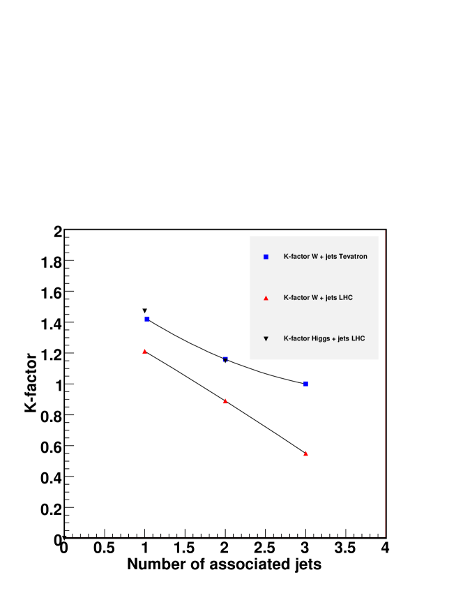
The K-factors for W + 1, 2 or 3 jets, at a renormalization/factorization scale of $m_{W}$, are plotted in Figure 1 (along with similar K-factors for Higgs + 1 or 2 jets)  [28]. In this plot, a pattern becomes obvious. The K-factors appear to decrease linearly as the number of final state jets increases, with a similar slope at the Tevatron as at the LHC (but with an offset). A similar slope is observed for Higgs boson+ jets at the LHC. To further understand this pattern (in addition to the color flow argument discussed in the previous section), we first have to review jet algorithms at LO and NLO.

At LO, one parton equals one jet. By choosing a jet algorithm with size parameter D, we are requiring any two partons to be a distance D or greater apart. The matrix elements have $1/\Delta R$ poles, so a larger value of D means smaller cross sections. At NLO, there can be two partons in a jet, and jets for the first time can have some structure. No $\Delta R$ cut is needed since the virtual corrections cancel the collinear singularity from the gluon emission (but there are residual logs that can become important if the value of D is too small). Increasing the size parameter D increases the phase space for including an extra gluon in the jet, and thus increases the cross section at NLO (in most cases). The larger the number of final state partons, the greater the differences will be between the LO and NLO dependence on jet size. The other factors mentioned above (such as the color arguments) are also important, but the impact of the jet algorithms at LO and NLO will become increasingly important for NLO calculations with large numbers of final-state partons.

Figure 1: The K-factors (NLO/LO) are plotted for $W$ production at the Tevatron and LHC and for Higgs production at the LHC as a function of the number of accompanying jets. The $k_{T}$ jet algorithm with a D parameter of 0.4 has been used.

It has been observed that the use of $\it typical$ scales for $W$ + 3 jet production at LO can result in substantial shape differences between the LO and NLO predictions [18, 17]. Conversely, the use of other scales, such as the sum of the transverse momentum of all final state objects ($H_{T}$), or the use of dynamically generated scales, such as with the CKKW or MLM procedures, result in good agreement between the LO and NLO predictions. A contribution (see S. Hoche et al) compares the results of different scale choices at LO and NLO for this final state (as well as being first direct comparison of the Rocket and Blackhat calculations).

An important search channel for Higgs boson production at the LHC is Vector Boson Fusion (VBF). The experimental signature consists of the presence of two forward-backward tag jets, and the suppression of additional hadronic activity in the central rapidity region. A comparison was made (in the contribution of A. Denner et al) between NLO predictions for this final state and leading order parton shower predictions. Differences between the two can partially be taken into account by the re-weighting of Herwig events, using a weight that depends on the transverse momentum of the Higgs boson.

The pattern of gluon radiation for a final state consisting of (1) a $W$ boson plus multiple jets (see J. Andersen et al) and (2) a Higgs boson plus multiple jets (see J. Andersen et al) was examined in these proceedings, with comparison of NLO calculations with LO + parton shower predictions and with the predictions of a BFKL Monte Carlo. A universal behaviour is observed for a strong correlation between the rapidity span (of the two most forward-backward jets) and the jet activity between these two jets. This implies that information about jet vetoes in Higgs boson production in association with dijets can be extracted from measurements in $W$ boson + dijets.

There was a great deal of discussion at Les Houches, and several resulting contributions, on the standardization of parton distribution functions (PDFs) and their uncertainties, and a quantitative understanding on reasons for any differences among PDFs produced by the major global PDF groups. The NNPDF group presented a study on the correlation between $\alpha_{s}(M_{Z})$ and the gluon distribution (see R. Ball et al); they found that, at least within the NNPDF approach, the sum in quadrature of PDF and $\alpha_{s}$ uncertainties provides an excellent approximation of that obtained from an exact error propagation treatment. For the case of Higgs boson production through $gg$ fusion, similar PDF uncertainties were found for CTEQ6.6 and MSTW2008, over a Higgs boson mass range of 100-300 GeV, with slightly larger uncertainties from the NNPDF1.2 PDFs.

A benchmarking study for heavy quark schemes was carried out at and after Les Houches (see the contribution of J. Rojo et al). The study compared quantitatively different General-Mass Variable Flavour Number (GM-VFN) schemes for the treatment of heavy quarks in deep-inelastic scattering. GM-VFN schemes used by the three main global PDF fitting groups were compared, and benchmark tables provided for easy comparison with any future GM-VFN schemes.

Although much of the work at Les Houches dealt with the impact of NLO corrections on LHC and Tevatron cross sections, many important cross sections have also been calculated at NNLO, and the extra order can provide additional important information. Higgs searches have been ongoing at the Tevatron for many years, with the $gg\rightarrow Higgs(\rightarrow WW)$ channel being the most promising in the Higgs mass range of approximately twice the $W$ mass. In one contribution, the impact of the NNLO corrections on the above channel (with the $W$ bosons decaying to leptons) was examined (see the contribution of G. Dissertori and F. Stockli). In the contribution of R. Boughezal, new NNLO predictions for Higgs boson production at the Tevatron,taking into account electroweak corrections in addition, were summarized. The new predictions are typically 4-6% lower than those previously used for Tevatron exclusion limits. In the contribution of G. Passarino, the complete NLO EW corrections to the (gg) Higgs production cross section were reviewed. Two schemes for including higher order EW corrections were discussed and Higgs pseudo-observables were introduced.

Some of the most precise determinations of the strong coupling constant result from measurements at $e^{+}e^{-}$ colliders, especially LEP. A contribution to Les Houches (see G. Dissertori et al) describes a precise determination of the strong coupling constant based on a NNLO+NNLA analysis of hadronic events shapes.

A combined theoretical/experimental study of the Frixione photon isolation scheme was carried out in the context of the Les Houches workshop. The finite size of the calorimeter cells into which fragmentation energy can be deposited was taken into account in the Frixione isolation scheme by introducing a finite number of nested cones together with the corresponding maximal values for the transverse energy allowed inside each of the cones. Together with novel techniques for the experimental estimation of the amount of underlying event/pileup transverse energy inside the isolation cone, this technique will allow for comparisons to theoretical calculations where the fragmentation component need not be calculated.

Finally, we would like to say that this group, and these proceedings, would not have been a success without the efforts of our colleague and co-convener, Thomas Binoth, who has left us far too soon. We would like to dedicate these proceedings to him.

Part I NLO TECHNIQUES, STANDARDIZATION, AUTOMATION

2 RECENT ADVANCES IN ANALYTIC COMPUTATIONS FOR ONE-LOOP AMPLITUDES

2.1 Introduction

Key insights of recent years have sparked progress in both analytic and numerical techniques for the computation of multi-particle one-loop amplitudes. Fully analytic computations offer the possibility of extremely fast and accurate evaluation of NLO cross-sections. Details of the analytic structure of the amplitudes, universal factorisation and cancellation of unphysical poles play an important role in the development of fully numerical methods. Further interplay between the two approaches would be useful to find the most flexible and efficient tools for NLO processes at the LHC. Achievements of new methods in numerical computation are presented elsewhere in this report. In this section we summarise recent developments in analytic computations.

Most current techniques involve unitarity cuts and generalised cuts, which are evaluated in regions of phase space where loop propagators are on shell. The expansion of the amplitude in master integrals with rational coefficients can then be evaluated algebraically in terms of tree-level quantities. Unlike in traditional reduction, individual coefficients are derived independently, based on the known analytic structure of the master integrals. A demonstration of the strength of analytic methods at one-loop was seen in the full computation of the six-gluon amplitude, whose components have been helpfully consolidated in [29]. A recent achievement, which we describe below, is the completion of all helicity amplitudes for the production of Higgs plus two jets [30, 8, 31, 32, 33, 34, 35, 36, 37].

2.2 INTEGRAL COEFFICIENTS FROM DOUBLE CUTS

The familiar “double” unitarity cuts (two propagators on shell) yield complete information about large classes of amplitudes. This cut-constructibility underlies the unitarity method of [38, 39] for finding coefficients of the master integrals without reducing Feynman integrals. “Spinor integration” methods, based on Cauchy’s residue theorem applied to the unitarity cut, have recently been used to generate closed-form expressions for the coefficients of scalar master integrals [40, 41, 42, 43]. The first such formulae [40, 41] were produced for 4-dimensional master integrals in massless theories, starting from tree-level input (the cut integrand) manifesting only physical singularities. From the integrand, the coefficients are obtained through a series of algebraic replacements. The formulae have been generalised to $D$-dimensional integrals in [44] and to scalar masses in [42].

The cut integrand, written analytically as a product of tree-level amplitudes, may be derived in a very compact form using “MHV diagrams” [45, 46, 47, 48, 49, 50, 51, 52, 53] or on-shell recursion relations, particularly in four dimensions with at least two massless particles involved in each tree amplitude [54, 55, 56, 57, 58, 59, 60, 61, 62, 63, 64, 65, 66, 67, 68, 69, 70]. Extensions to dimensions other than four have been explored in [71, 72, 73, 74]. However, on-shell recursion relations typically feature unphysical singularities, “spurious poles”, in their individual terms. In [43], the closed form coefficients of [42] have been generalised to allow any rational functions as cut integrands, in particular with the possible presence of spurious poles.

Current techniques of evaluating unitarity cuts permit numerous variations. As mentioned above, the cuts may be evaluated by the residue theorem each time, incorporating simplifications depending on the specific forms of the integrands; or the available closed forms for coefficients may be used blindly. Certainly, there are intermediate and related approaches as well, which are being explored for optimal efficiency, considering also numerical evaluations. A recent study [75] frames the double-cut phase space integral in terms of Stokes’ theorem, bypassing spinors in favour of a conjugate pair of complex scalar integration variables. The cut is evaluated by indefinite integration in one variable followed by Cauchy’s residue theorem applied to the conjugate variable. The cuts of bubble integrals are rational functions, so their coefficients may be extracted algebraically by Hermite polynomial reduction. It has also been observed that a unitarity cut, viewed as the imaginary part of the loop amplitude, may be interpreted as a Berry phase of the effective momentum space experienced by the two on-shell particles going around the loop [76]. The result of the phase-space integration is thus the flux of a 2-form given by the product of the two tree amplitudes on either side of the cut.

2.3 GENERALISED UNITARITY

Generalised unitarity has become an essential tool in the computation of one-loop amplitudes over the past two years. Analytic techniques have focused on generalisations to full QCD amplitudes with arbitrary internal and external masses.

Multiple cuts are well established as an efficient method for the computation of one-loop amplitudes [77]. The quadruple cut technique [78] isolates box coefficients in the one-loop basis, reducing computation to an algebraic procedure. Forde’s Laurent expansion technique [79] has been widely used in numerical applications and has also been generalised to the massive case [80]. Further understanding into the analytic structure has led to the interpretation of the triple cut [81] and double cut [75] in terms of Cauchy’s and Stokes’s Theorem respectively.

$D$-dimensional cuts with generalised unitarity have also been applied to analytic computations [82] using the well known interpretation of the $D$-dimensional loop integral as a massive vector [83, 84]. In contrast to numerical applications [84, 85], this allows for a direct computation of the rational contributions without the need to compute quintuple cuts.

Although the $D$-dimensional cutting method is completely general, in some cases it is preferable to use on-shell recursion relations for the rational terms [86]. As long as a suitable analytic continuation can be found which avoids non-factorising channels, extremely compact analytic forms can be obtained [87, 88, 35, 33, 34]. Recently combinations of these techniques have been applied in the context of $H+2j$ productions [35, 36, 37] and in preliminary studies of $t\bar{t}$ production [89]. Since the methods are all completely algebraic, they are particularly suitable for automation with compact tree-level input taken from on-shell recursion.

For massive one-loop amplitudes, the analytic structure is less understood than in the massless case. In particular, the addition of wave-function and tadpole contributions introduces complications, as these integrals lack four-dimensional branch cuts in momentum channels. A recent analysis proposes computing tadpole coefficients from coefficients of higher-point integrals by introducing an auxiliary, unphysical propagator [90]. The original tadpole integral is then related to an auxiliary integral with two propagators, which can be treated by a conventional double cut. Relations have been found giving the tadpole coefficients in terms of the bubble coefficients of both the original and auxiliary integrals, and the triangle coefficients of the auxiliary integrals. The proof of these relations is accomplished with the help of the integrand classification of [91].

Single cuts, used in conjunction with generalised cutting principles, can be an effective method for deriving full QCD amplitudes [92]. A different single-cut method, proposed as an alternative to generalised unitarity cuts, relies on a “dual” prescription for the imaginary parts of propagators [93].

2.4 COMPACT ANALYTIC EXPRESSIONS FOR HIGGS PLUS TWO JETS

The program of completing the computation of all helicity amplitudes for $H+2j$ production at Hadron colliders as recently been completed. This allows for a much faster evaluation (about 10 ms for the full colour/helicity sum) of the cross-section previously available from a semi-numerical computation [30, 8]. A wide variety of the techniques listed above were employed to ensure a compact analytic form.

The calculation was performed in the large top-mass limit where the Higgs couples to the gluons through an effective dimension five operator. A complex Higgs field was decomposed into self-dual ($\phi$) and anti-self-dual ($\phi^{\dagger}$) pieces from which the standard model amplitudes can be constructed from the sum of $\phi$ and parity symmetric $\phi^{\dagger}$ amplitudes,

$$A(H,\{p_{k}\})=A(\phi,\{p_{k}\})+A(\phi^{\dagger},\{p_{k}\}).$$ (1)

Helicity amplitudes have been calculated using the standard 2-component Weyl spinor representations and written in terms of spinor products. Results are presented unrenormalised in the four dimensional helicity scheme.

2.5 Full analytic results

The full set of amplitudes collects together the work from a number of different groups which we summarise below:

$H\rightarrow gggg$
Helicity	$\phi$	$\phi^{\dagger}$
$----$	[31]	[32]
$+---$	[36]	[32]
$--++$	[33]	[33]
$-+-+$	[34]	[34]

$H\rightarrow\bar{q}qgg$
Helicity	$\phi$	$\phi^{\dagger}$
$-++-$	[35]	[35]
$-+-+$	[35]	[35]
$-+--$	[37]	[32]

Table 3: The set of independent $\phi$ and $\phi^{\dagger}$ helicity amplitudes contributing to $H+2j$ production together with the references where they can be obtained.

The analytic form of the four quark squared amplitude was presented in the original semi-numerical computation [30]. The helicity amplitudes for this process were computed in reference [35]. The results where obtained using 4-dimensional cutting techniques for the cut-constructible parts. Where applicable on-shell recursion relations gave a compact representation of the rational terms. For the most complicated NMHV configuration and the “all-minus" configuration non-factorising channels in the complex plane were unavoidable and on-shell recursion was not possible. In these cases extremely compact forms were obtained from Feynman diagrams after all information from unphysical poles in the cut-constructible part had been accounted for. It was essential to make full use of the universal IR pole structure in addition to information coming from spurious poles in the logarithmic part.

This calculation relied on some non-trivial relations between terms in the amplitude:

• The rational terms in the $\phi gggg$ amplitude obey:

  $$\mathcal{R}\left\{A_{4;1}(\phi;1_{g},2_{g},3_{g},4_{g})\right\}=\left(1-\frac{N_{f}}{N_{c}}+\frac{N_{s}}{N_{c}}\right)R^{N_{p}}(\phi;1_{g},2_{g},3_{g},4_{g})$$

  $$+2\left(A_{4}^{(0)}(\phi,1_{g},2_{g},3_{g},4_{g})-A_{4}^{(0)}(\phi^{\dagger},1_{g},2_{g},3_{g},4_{g})\right)$$ (2)

• The rational terms in the $\phi\bar{q}qgg$ amplitude obey:

  $$\mathcal{R}\bigg{\{}A_{4}^{L}(\phi;1_{\bar{q}},2_{q},3_{g},4_{g})+A_{4}^{R}(\phi;1_{\bar{q}},2_{q},3_{g},4_{g})+A_{4}^{f}(\phi;1_{\bar{q}},2_{q},3_{g},4_{g})\bigg{\}}$$

  $$=2\left(A_{4}^{(0)}(\phi,1_{\bar{q}},2_{q},3_{g},4_{g})-A_{4}^{(0)}(\phi^{\dagger},1_{\bar{q}},2_{q},3_{g},4_{g})\right)$$ (3)

• The sub-leading colour amplitudes in the $H\bar{q}qgg$ amplitude are completely determined from the leading singularities.

The identities are strongly reminiscent of cancellations seen in SUSY decompositions of pure QCD amplitudes except that they are broken by a universal factor proportional to the tree-level $\phi$ and $\phi^{\dagger}$ amplitudes.

As an example we present the colour ordered amplitude for the most complicated “NMHV" configuration in the $Hgggg$ channel [36]. The Feynman diagram representation of this amplitude consists of 739 diagrams with up to rank 4 tensor pentagon integrals. This leading colour amplitude is sufficient to give the full colour information when summed over the appropriate permutations, we refer the reader to [36] for further details.

$$A^{(1)}_{4;1}(H,1^{+},2^{-},3^{-},4^{-}) = -A^{(0)}_{4}(H,1^{+},2^{-},3^{-},4^{-})\sum_{i=1}^{4}\frac{1}{\epsilon^{2}}\left(\frac{\mu_{R}^{2}}{-s_{i,i+1}}\right)^{\epsilon}$$ (4)

$$+ F_{4}(H,1^{+},2^{-},3^{-},4^{-})+R_{4}(H,1^{+},2^{-},3^{-},4^{-})$$

where

$$A^{(0)}_{4}(H,1^{+},2^{-},3^{-},4^{-})=$$

$$-\frac{m_{H}^{4}\langle 24\rangle^{4}}{s_{124}\langle 12\rangle\langle 14\rangle\langle 2|p_{H}|3]\langle 4|p_{H}|3]}+\frac{\langle 4|p_{H}|1]^{3}}{s_{123}\langle 4|p_{H}|3][12][23]}-\frac{\langle 2|p_{H}|1]^{3}}{s_{134}\langle 2|p_{H}|3][14][34]},$$ (5)

and

$$F_{4}(H,1^{+},2^{-},3^{-},4^{-})=\bigg{\{}\frac{1}{4s_{124}}\bigg{(}\frac{\langle 3|p_{H}|1]^{4}}{\langle 3|p_{H}|2]\langle 3|p_{H}|4][21][41]}+\frac{\langle 24\rangle^{4}m_{H}^{4}}{\langle 12\rangle\langle 14\rangle\langle 2|p_{H}|3]\langle 4|p_{H}|3]}\bigg{)}W^{(3)}$$

$$-\frac{s_{234}^{3}}{4\langle 1|p_{H}|2]\langle 1|p_{H}|4][23][34]}W^{(1)}-\bigg{(}\frac{\langle 2|p_{H}|1]^{3}}{2s_{134}\langle 2|p_{H}|3][34][41]}+\frac{\langle 34\rangle^{3}m_{H}^{4}}{2s_{134}\langle 1|p_{H}|2]\langle 3|p_{H}|2]\langle 41\rangle}\bigg{)}W^{(2)}$$

$$+2C_{3;H|12|34}^{\rm 3m}(1^{+},2^{-},3^{-},4^{-}){\rm I_{3}^{3m}}(m_{H}^{2},s_{12},s_{34})+\left(1-\frac{N_{f}}{4N_{c}}\right)\bigg{(}\frac{\langle 3|p_{H}|1]^{2}}{s_{124}[24]^{2}}{\rm F^{1m}}(s_{12},s_{14};s_{124})$$

$$-\frac{4\langle 24\rangle\langle 3|p_{H}|1]^{2}}{s_{124}[42]}\hat{L}_{1}\left(s_{124},s_{12}\right)+\frac{4\langle 23\rangle\langle 4|p_{H}|1]^{2}}{s_{123}[32]}\hat{L}_{1}\left(s_{123},s_{12}\right)\bigg{)}-\bigg{(}1-\frac{N_{f}}{N_{c}}+\frac{N_{s}}{N_{c}}\bigg{)}\times$$

$$\bigg{(}\frac{[12][41]\langle 3|p_{H}|2]\langle 3|p_{H}|4]}{2s_{124}[24]^{4}}{\rm F^{1m}}(s_{12},s_{14};s_{124})+\left(\frac{2s_{124}\langle 34\rangle^{2}[41]^{2}}{\langle 24\rangle[42]^{3}}-\frac{\langle 24\rangle\langle 3|p_{H}|1]^{2}}{3s_{124}[42]}\right)\hat{L}_{1}\left(s_{124},s_{12}\right)$$

$$+\frac{2s_{124}\langle 24\rangle\langle 34\rangle^{2}[41]^{2}}{3[42]}\hat{L}_{3}\left(s_{124},s_{12}\right)+\frac{\langle 34\rangle[41]\left(3s_{124}\langle 34\rangle[41]+\langle 24\rangle\langle 3|p_{H}|1][42]\right)}{3[42]^{2}}\hat{L}_{2}\left(s_{124},s_{12}\right)$$

$$+\frac{\langle 3|p_{H}|1](4s_{124}\langle 34\rangle[41]+\langle 3|p_{H}|1](2s_{14}+s_{24})}{s_{124}\langle 24\rangle[42]^{3}}\hat{L}_{0}\left(s_{124},s_{12}\right)-\frac{2s_{123}\langle 23\rangle\langle 34\rangle^{2}[31]^{2}}{3[32]}\hat{L}_{3}\left(s_{123},s_{12}\right)$$

$$+\frac{\langle 23\rangle\langle 34\rangle[31]\langle 4|p_{H}|1]}{3[32]}\hat{L}_{2}\left(s_{123},s_{12}\right)+\frac{\langle 23\rangle\langle 4|p_{H}|1]^{2}}{3s_{123}[32]}\hat{L}_{1}\left(s_{123},s_{12}\right)\bigg{)}\bigg{\}}+\bigg{\{}(2\leftrightarrow 4)\bigg{\}}.$$ (6)

For convenience we have introduced the following combinations of the finite pieces of one-mass $({\rm F^{1m}})$ and two-mass hard $({\rm F^{2mh}})$ box functions,

$$W^{(1)} = {\rm F^{1m}}(s_{23},s_{34};s_{234})+{\rm F^{2mh}}(s_{41},s_{234};m_{H}^{2},s_{23})+{\rm F^{2mh}}(s_{12},s_{234};s_{34},m_{H}^{2})$$

$$W^{(2)} = {\rm F^{1m}}(s_{14},s_{34};s_{134})+{\rm F^{2mh}}(s_{12},s_{134};m_{H}^{2},s_{34})+{\rm F^{2mh}}(s_{23},s_{134};s_{14},m_{H}^{2})$$

$$W^{(3)} = {\rm F^{1m}}(s_{12},s_{14};s_{124})+{\rm F^{2mh}}(s_{23},s_{124};m_{H}^{2},s_{14})+{\rm F^{2mh}}(s_{34},s_{124};s_{12},m_{H}^{2}).$$

The bubble coefficients have been re-arranged into logarithm functions, $L_{k}=\frac{\log(s/t)}{(s-t)^{k}}$, which have smooth behaviour in the various collinear limits,

$$\hat{L}_{3}(s,t) = L_{3}(s,t)-\frac{1}{2(s-t)^{2}}\bigg{(}\frac{1}{s}+\frac{1}{t}\bigg{)}\quad,\quad\hat{L}_{1}(s,t)=L_{1}(s,t),$$

$$\hat{L}_{2}(s,t) = L_{2}(s,t)-\frac{1}{2(s-t)}\bigg{(}\frac{1}{s}+\frac{1}{t}\bigg{)}\quad,\quad\hat{L}_{0}(s,t)=L_{0}(s,t).$$ (7)

Representations for the scalar integrals can be found in the literature [94, 95, 96, 97]. The three mass triangle coefficient was obtained from Forde’s Laurent expansion procedure [79],

$$C_{3;H|12|34}^{\rm 3m}(1^{+},2^{-},3^{-},4^{-})=\sum_{\gamma=\gamma_{\pm}(p_{H},p_{1}+p_{2})}\frac{-m_{\phi}^{4}\langle K^{\flat}_{1}2\rangle^{3}\langle 34\rangle^{3}}{2\gamma(\gamma+m_{\phi}^{2})\langle{K^{\flat}_{1}}{1}\rangle\langle{K^{\flat}_{1}}{3}\rangle\langle{K^{\flat}_{1}}{4}\rangle\langle 12\rangle},$$ (8)

where $K_{1}=p_{H},K_{2}=p_{1}+p_{2}$, and

$$K^{\flat,\mu}_{1} = \gamma\frac{\gamma K_{1}^{\mu}-K_{1}^{2}K_{2}^{\mu}}{\gamma^{2}-K_{1}^{2}K_{2}^{2}},\quad K^{\flat,\mu}_{2}=\gamma\frac{\gamma K_{2}^{\mu}-K_{2}^{2}K_{1}^{\mu}}{\gamma^{2}-K_{1}^{2}K_{2}^{2}},$$

$$\gamma_{\pm}(K_{1},K_{2}) = K_{1}\cdot K_{2}\pm\sqrt{K_{1}\cdot K_{2}^{2}-K_{1}^{2}K_{2}^{2}}.$$ (9)

The rational part (which incorporates the rational $A^{(1)}_{4}(\phi^{\dagger},1^{+},2^{-},3^{-},4^{-})$ amplitude derived in [32]) is

$$R_{4}(H,1^{+},2^{-},3^{-},4^{-})= \bigg{\{}\bigg{(}1-\frac{N_{f}}{N_{c}}+\frac{N_{s}}{N_{c}}\bigg{)}\frac{1}{2}\bigg{(}\frac{\langle 23\rangle\langle 34\rangle\langle 4|p_{H}|1][31]}{3s_{123}\langle 12\rangle[21][32]}-\frac{\langle 3|p_{H}|1]^{2}}{s_{124}[42]^{2}}$$ (10)

$$+\frac{\langle 24\rangle\langle 34\rangle\langle 3|p_{H}|1][41]}{3s_{124}s_{12}[42]}-\frac{[12]^{2}\langle 23\rangle^{2}}{s_{14}[42]^{2}}-\frac{\langle 24\rangle(s_{23}s_{24}+s_{23}s_{34}+s_{24}s_{34})}{3\langle 12\rangle\langle 14\rangle[23][34][42]}$$

$$+\frac{\langle 2|p_{H}|1]\langle 4|p_{H}|1]}{3s_{234}[23][34]}-\frac{2[12]\langle 23\rangle[31]^{2}}{3[23]^{2}[41][34]}\bigg{)}\bigg{\}}+\bigg{\{}(2\leftrightarrow 4)\bigg{\}}.$$

Further study into the origin of the simplicity in the sub-leading colour amplitudes would be interesting and may shed light on possible cancellations in other processes [98]. The full results for all helicity configurations have been made available at http://mcfm.fnal.gov.

3 A GENERIC IMPLEMENTATION OF D-DIMENSIONAL UNITARITY

3.1 Introduction

Until recently, the computational bottleneck in next-to-leading order QCD calculations has been the evaluation of the virtual part of the partonic cross section. The mainstream technology for evaluating one loop integrals corresponding to one loop Feynman diagrams has been to project the contribution of each individual Feynman diagram on a complete basis of scalar master integrals that are known analytically. There are many generic frameworks implemented that have been used the last years in very demanding calculations (see for example [99, 100, 101] or the publically available [102].

Alternative approaches based on unitarity have been employed extensively in the past to recover one loop amplitudes (see e.g. [39, 38]). Following a generalization of the unitarity idea to quadruple cuts [78] and a novel approach in reduction that allows one to partially fraction numerically one loop integrals at the integrand level on a per point base [91, 103], the numerical evaluation of one loop amplitudes using tree-level quantities as building blocks appeared to be possible and efficient enough to tackle processes with many final state partons. Since then there have been mainly three approaches developed along the lines of numerical reduction with tree-level objects as building blocks: the Black Hat approach [104, 105](based also on the reduction method of [79], implemeneted in [105, 106]), the D-dimensional unitarity approach [107, 84, 108, 85] (implemented in various independent codes  [109, 110, 111, 112, 113] ) and the helac-1loop approach[103, 114, 115, 116, 117, 118, 119] (implemented in [120]). All three approaches have already delivered differential cross sections for processes of prime phenomenological importance [121, 122, 123, 17, 124, 16, 125, 111, 26, 126, 18].

In what follows I report on the progress of a generic implementation of the D-dimensional unitarity approach, emphasizing the particular points where my implementation differs from the published mainstream algorithm.

3.2 The main algorithm and variations.

Within the framework of dimensional regularization, one loop integrals are analytically continued in $D=4-2\epsilon$ dimensions. The particular way one treats this analytic continuation with respect to the degrees of freedom, $D_{s}$ of the unobserved particles that circulate in the loop defines the regularization scheme used. The fundamental idea of (generalized) D-dimensional unitarity is the observation that the amplitude depends on $D_{s}$ in a linear way, when the loop is not purely fermionic:

$$A^{D_{s}}=A_{0}+D_{s}A_{1}$$ (11)

When the loop is purely fermionic, the colour-ordered amplitude is just proportional to $2^{D_{s}/2}$:

$$A^{D_{s}}=2^{D_{s}/2}A_{0}$$ (12)

The strategy is to evaluate $A^{D_{s}}$ numerically for two integer dimensions $D_{s}$, extract $A_{0}$ and $A_{1}$. The full $D_{s}$ dependence of $A^{D_{s}}$ is then recovered and the amplitude can be evaluated in the regularization scheme of preference.

The lowest values of $D_{s}$ one needs to accommodate fermions are $D_{s}=6$ and $D_{s}=8$. Then

$$A_{0}=4A^{6}-3A^{8}\;\;\;\;A_{1}=\frac{A^{8}-A^{6}}{2}$$ (13)

Choosing the FDH scheme ($D_{s}=4$), the amplitude takes the form

$$A^{FDH}=2A^{6}-A^{8}$$ (14)

One would now normally set up two OPP systems, to evaluate $A^{6}$ and $A^{8}$ using the corresponding residues throughout. Instead, thanks to the linearity of the OPP system, one can evaluate directly $A^{FDH}$. The residues that appear on the left hand side of the OPP equations would now correspond to the difference $2A^{6}|_{res}-A^{8}|{res}$. Potential cancelations between the two contributions, which would have propagated in the coefficients of the OPP system, are now prevented.

The residue of the amplitude with respect to a given multiple cut is recognized [107] to be a product of tree-level amplitudes sewn together with a sum over polarization states of the particles corresponding to the cut propagators:

$$A^{D_{s}}|_{res}=\sum_{\lambda_{1},\ldots\lambda_{N}}(\bar{w}^{\lambda_{1}}_{\mu_{1}}M^{\mu_{1}\mu_{2}}w_{\mu_{2}}^{\lambda_{2}})(\bar{w}_{\mu_{2}}^{\lambda_{2}}M^{\mu_{2}\mu_{3}}w_{\mu_{3}}^{\lambda_{3}})\ldots(\bar{w}^{\lambda_{N}}_{\mu_{N}}M^{\mu_{N}\mu_{1}}w_{\mu_{1}}^{\lambda_{1}})$$ (15)

where $w_{\mu_{i}}^{\lambda^{i}}$ is the wave function of the cut particle (eg. a spinor for a fermion or a polarization vector for a gluon) corresponding to helicity $\lambda^{i}$. The tree level amplitudes are obtained via the Berends-Giele recursion relation. This, in effect, means that the current $J_{12}^{\mu_{2}}\equiv w^{\lambda_{1}}_{\mu_{1}}M^{\mu_{1}\mu_{2}}$ is evaluated numerically and then multiplied by the external wave function $\bar{w}_{\mu_{2}}^{\lambda_{2}}$ to get the amplitude as a complex number. A rather trivial but vastly simplifying observation is that one can perform the polarization sums in $N-1$ of the cut propagators and use the spin projectors to join the Berends-Giele currents. We then have

$$J_{k,k+1}^{\mu_{k+1}}=\tilde{J}_{k-1,k;\mu_{k}}M^{\mu_{k}\mu_{k+1}}\;\;\;\;\;\;\;\tilde{J}_{k-1,k;\mu_{k}}\equiv J_{k-1,k}^{\nu}D_{\nu,\mu_{k}}(p_{k})$$ (16)

with $D_{\nu,\mu_{k}}(p_{k})$ the spin projector for the cut particle $k$ carrying (loop) momentum $p_{k}$. This transforms the multiple sum of eq. 15 in a single sum over the polarization states of a single cut particle. One can see this schematically as a ring with a single polarization sum, similar (but not identical) to the way the calculation of residues is organized in the approach of [120]. As a side remark, choosing to sum over polarization states of another propagator would provide a non-trivial numerical test for the evaluation of the cut.

Regarding the computational burden of evaluating the rational part in extra dimensions, it is clear, from the representation of the Dirac algebra in $6$ and $8$ dimensions, and the fact that the loop momenta chosen are always restricted to $5$ dimensions, that $A^{8}|_{res}=A^{6}|_{res}+\hat{A}^{8}|_{res}$. In particular, in terms of the rings described above, $\hat{A}^{8}|_{res}=\sum_{h=5\ldots h_{max}^{8}}R_{h}$ where $h^{8}_{max}=6$ when the cut line is a gluon, and $h^{8}_{max}=8$ when the cut line is a fermion. Obviously it is advantageous to cut a gluon line when this is possible.

3.3 A note on numerical stability

Since D-dimensional unitarity involves pentuple cuts, it is exposed to a direct criticism regarding the numerical stability of the method, not only as far as the calculation of the rational part is concerned, but also in connection to the cut constructible part, which, in other methods, is evaluated in strictly four dimensions. In particular, pentagon coefficients, carrying inverse Gram determinants up to the fifth power, are potential sources of precision loss in phase space points that are close to configurations with co-planar momenta. The detection of such problematic points can be achieved with either comparing the evaluated pole coefficients (in an $\epsilon$-expansion of the amplitude) with those known from analytical formulas, or by checking redundant individual OPP systems for consistency. Both methods are used in the implementation described here.

The percentage of such problematic points depends on the number and type of external particles as well as the particular phase space cuts imposed. The most direct attitude towards this issue (aside from just discarding those points) is to evaluate them in double-double ($32$ digits) or quadruple ($64$ digits) precision using libraries available in the literature. Even though the percentage of problematic points is always less than $5\%$, the exact rate matters, since the penalty in terms of cpu time paid for the increased precision arithmetics can reach a factor of $100$.

An alternative approach that drastically increases precision for the cut constructible part of the amplitude (without losing information necessary for the rational part or evaluating extra residues) and slightly improves the behavior of the rational part is described in detail in [127]. The basic idea is to separate the pentagon contributions throughout the OPP system in another, separately solved system of equations. The remaining system contains the four-dimensional OPP system for the cut-constructible part. Moreover, the factorized pentagon coefficients can be manipulated easily, taking care to avoid numerical cancellations.

3.4 Summary

The present implementation of D-dimensional unitarity is restricted to amplitudes relevant for NLO QCD calculations with massless particles. In terms of color ordered primitives, the full gluonic primitive, primitives with one or more fermion lines and primitives with closed fermion loops are all implemented and checked either by verifying their singularity structure or against published results. The implementation is independent of the number of external particles. Further details about primitives not available in the literature will be given in a forthcoming publication. The numerical stability of the algorithm is enhanced since the effect of large pentagon coefficients is reduced. A number of modifications from the main algorithm that were described above, help to improve the accuracy as well as the computational complexity of the method.

4 ANALYTICAL CALCULATION OF THE RATIONAL PART OF 1-LOOP AMPLITUDES: THE R2 CONTRIBUTION

The automatic computation of beyond-leading-order amplitudes for processes involving multiparticle production in the framework of the $\mathrm{SU(3)_{C}\times SU(2)_{W}\times U(1)_{Y}}$ Standard Model (SM) of interactions, is one of the goals of the present developments in Theoretical Physics at High-Energy Colliders. The demand for (at least) NLO predictions for partonic processes is an established issue [128], since processes with many external legs (jets) are expected at the LHC [129] and LO predictions can suffer of uncertainties, like renormalization and factorization scale dependencies, which can increase with the number of external legs. Thus, recently, some of the current available Matrix-Element MonteCarlo (MC) event generators, such as HELAC/PHEGAS [130] and SHERPA [131, 132], used even by the experimental community in the prediction of inclusive and exclusive observables of interest, have been interfaced with proper codes for the automatic evaluation of 1-loop correction contributions [120, 123]. This work has just started, and, even if it has already allowed to get theoretical predictions for most of the specific processes and sub-processes suggested by the 2007 Les Houches wishlist [3], has not yet achieved the stage of a completely automatic and systematic evaluation.

Even if interesting results (see e.g. [14]) have been obtained also in the context of the traditional Passarino-Veltman reduction technique [133], many of the methods recently developed for the evaluation of virtual contributions at NLO [134], that have pushed crucial progresses in this field, are based on Unitarity arguments [135, 136, 77]. Due to the unitarity of the S-matrix, it is always possible to express any 1-loop amplitude, for any given number of external legs, as a linear combination of 1-loop scalar functions up to 4 external legs (boxes, triangles, bubbles and, eventually, tadpoles), i.e. the cut-constructible (CC) part, plus a residual piece, called the rational part (R). Since libraries for the evaluation of these well-known scalar integrals exist [96, 97], the problem of determining a 1-loop amplitude is reduced to the one of determining the coefficients of the combination and of evaluating the residual piece. One of the methods developed so far for the determination of these coefficients is the OPP reduction [91]. According to it, the coefficients of the expansion of the amplitude in terms of scalar integrals are obtained by working at the integrand level in a completely algebraic way, indipendently of the theory of interactions at hand, i.e. the method can be applied to any renormalizable gauge theory. Both massless and massive particles can be included in the loop. The method does not require to introduce any additional integer dimension beyond the four we are used to consider in special relativity.

As for the residual piece, in the OPP framework, two kinds of R terms have been recognized, denoted by ${\rm R_{1}}$ and $\rm{R_{2}}$, respectively [114]. The ${\rm R_{1}}$ terms come essentially from the D-dimensional dependence of the denominators appearing in the integrands of 1-loop amplitudes, when one applies a dimensional regularization procedure (working in D = $4+\epsilon$ dim.) to calculate the amplitudes themselves. In fact, in the OPP reduction procedure aimed to obtain the CC part, the denominators are treated as 4-dimensional, by neglecting their D-dimensional dependence. The $\rm{R_{2}}$ terms, instead, come from the $\epsilon$-dimensional part of the numerators.

In the OPP framework, the ${\rm R_{1}}$ contribution can be reconstructed at the same time of the CC part, without needing to know the analytical structure of the amplitude, i.e. the contributing Feynman diagrams. In other words, to build the CC part and the ${\rm R_{1}}$ part of the amplitudes, it is enough to know the numerator of the integrand in four dimensions as a numerical function of the loop momentum $q$, and this numerator $N(q)$ can already include the sum of many contributions, corresponding to different loop particle contributions, given a fixed structure of external legs.

On the other hand, the numerical knowledge of $N(q)$ is not enough to extrapolate the $\epsilon$-dependence of the numerator, i.e. the $\rm{R_{2}}$ terms have to be calculated separately. The strategy we have adopted so far to build $\rm{R_{2}}$ is based on the consideration that the divergencies appearing in the $\rm{R_{2}}$ integrands that have to be regularized have a completely ultraviolet (UV) nature [137]. Thus, irreducible $\rm{R_{2}}$ contributions up to four external legs are enough to build the total $\rm{R_{2}}$ for processes with any number of external legs. Since the number of $\rm{R_{2}}$ building-blocks is finite, it is possible to write them in the form of effective Feynman rules, derived for each of the theories of particle interactions at hand. We have first derived these Feynman rules in the framework of QCD, where the number of involved particles is relatively low, thus only a few effective vertices exist [118]. We have provided these rules both in the ’t Hooft-Feynman gauge and in the Four Dimensional Helicity (FDH) scheme, which is a particular case of the previous one, corresponding to selecting only a part of the rational terms ($\epsilon$ is set to 0 before integration). The rules have been derived analytically by using FORM [138, 139]. We have then extended the list of effective Feynman rules, by adding the ones for 1-loop QCD corrections to Electroweak (EW) amplitudes, the ones for EW corrections to QCD amplitudes and, finally, the ones for EW corrections to EW processes [119].

We have tested our analytical results, by considering the fact that $\rm{R_{2}}$ is not gauge invariant by itself, but the sum ${\rm R_{1}}$+$\rm{R_{2}}$ has to fulfill this constraint, i.e. a given set of Ward identities [140] has to be satisfied. We have derived these Ward identities in the formalism of the Background Field Method (BFM) [141, 142]. We have derived analytical formulas for ${\rm R_{1}}$ terms up to 4-external legs, and we have verified that the sums ${\rm R_{1}}$+$\rm{R_{2}}$ satisfy the Ward identities. This can be considered a non-trivial test, since the analytical expressions of ${\rm R_{1}}$ effective vertices are in general much more complicated, by involving many terms, with denominators including different combinations of the momenta of the external particles. It is worth mentioning that, at the aim of calculating ${\rm R_{1}}$ for an arbitrary process, it is not possible to apply a procedure, based on Feynman rules, analogous to the one used to calculate $\rm{R_{2}}$, since, in case of many external legs, one cannot rely on ${\rm R_{1}}$ contributions up to 4-external legs only. Furthermore, the analytical structure of the ${\rm R_{1}}$ terms becomes soon very complicated by increasing the number of external legs, thus, in general, it is easier to proceed with a numerical evaluation of ${\rm R_{1}}$.

As an explicit and simple example of the procedure we have adopted to derive the ${\rm{R_{2}}}$ effective Feynman rules, we detail the calculation of ${\rm{R_{2}}}$ coming from the gluon self-energy. The contributing diagrams are drawn in fig. 2.

As for the ghost loop with 2 external gluons, we can write the numerator as

$$\bar{N}(\bar{q})=\frac{g^{2}}{(2\pi)^{4}}f^{a_{1}bc}\,f^{a_{2}cb}\,(p+\bar{q})^{\mu_{1}}\bar{q}^{\mu_{2}}\,.$$ (17)

In the previous equation, dimensional regularization is assumed, so that we use a bar to denote objects living in $D=~{}4+\epsilon$ dimensions. Notice that, when a $D$-dimensional index is contracted with a 4-dimensional (observable) vector $v_{\mu}$, the $4$-dimensional part is automatically selected. For example,

$$\bar{q}\cdot v\equiv(q+{\tilde{q}})\cdot v\,=q\cdot v\,~{}~{}~{}{\rm and}~{}~{}~{}\hbox to0.0pt{/\hss}{\bar{v}}\equiv\bar{\gamma}_{\bar{\mu}}\,v^{\mu}=\hbox to0.0pt{/\hss}v\,,$$ (18)

where we have used a tilde to represent $\epsilon$-dimensional quantities. Since $\mu_{1}$ and $\mu_{2}$ are external Lorentz indices, that are eventually contracted with 4-dimensional external currents, their $\epsilon$-dimensional component is killed due to eq. 18. Therefore, ${\rm{R_{2}}}=0$ for this diagram, being the $\epsilon$-dependent part of the numerator $\tilde{N}(\tilde{q}^{2},q,\epsilon)=0$. With analogous arguments, one easily shows that ghost loops never contribute to ${\rm{R_{2}}}$, even in case of 3 or 4 external gluons. This is not only the case of QCD ghosts, but even the one of EW ghosts that enter EW loops. In general, loops of ghost particles give instead a non-vanishing contribution to ${\rm R_{1}}$.

The contribution due to $N_{f}$ quark loops is given by the second diagram of fig. 2, whose numerator reads

$$\bar{N}(\bar{q}) = -\frac{g^{2}}{(2\pi)^{4}}N_{f}\frac{\delta_{a_{1}a_{2}}}{2}\,Tr[{\gamma}^{{\mu_{1}}}(\hbox to0.0pt{/\hss}{\bar{q}}+m_{q}){\gamma}^{{\mu_{2}}}(\hbox to0.0pt{/\hss}{\bar{q}}+\hbox to0.0pt{/\hss}{p}+m_{q})]\,,$$ (19)

where the external indices $\mu_{1}$ and $\mu_{2}$ have been directly taken in 4 dimensions. By anti-commuting ${\gamma}^{{\mu_{2}}}$ and $\hbox to0.0pt{/\hss}{\bar{q}}$ and using the fact that, due to Lorentz invariance, odd powers of ${\tilde{q}}$ do not contribute, one immediately get the result

$$\tilde{N}({\tilde{q}}^{2})=\frac{g^{2}}{8\pi^{4}}\,N_{f}\,\delta_{a_{1}a_{2}}\,g_{\mu_{1}\mu_{2}}{\tilde{q}}^{2}\,.$$ (20)

Eq. 20, integrated with the help of the eq.

$$\int d^{n}\bar{q}\frac{\tilde{q}^{2}}{\bar{D}_{i}\bar{D}_{j}} = -\frac{i\pi^{2}}{2}\left[m_{i}^{2}+m_{j}^{2}-\frac{(p_{i}-p_{j})^{2}}{3}\right]+O(\epsilon)\,,$$ (21)

where $\bar{D}_{i}=(p_{i}+\bar{q})^{2}-m_{i}^{2}$, gives the term proportional to $N_{f}$ in the 2-point effective vertex of fig. 3.

Figure 2: Diagrams contributing to the gluon self-energy.

Figure 3: $\rm{R_{2}}$ gluon-gluon effective vertex. $\lambda_{HV}=1$ in the ’t Hooft-Feynman scheme and $\lambda_{HV}=0$ in the FDH scheme. $N_{col}$ is the number of colors and $N_{f}$ is the number of fermions running in the quark loop.

The effective rules providing the QCD NLO $\rm{R_{2}}$ corrections have already been implemented in a numerical code based on tensor reduction [143]. Furthermore, they have been used in a unitary context by the HELAC-NLO system, in the study of NLO processes like $pp\rightarrow t\bar{t}b\bar{b}$ [16] and $pp\rightarrow t\bar{t}H$, with the Higgs boson subsequently decaying in $b\bar{b}$ [144]. At the purpose of calculating the total $\rm{R_{2}}$ contribution to a physical process, these Feynman rules have to be considered on the same footing as the standard ones. The only constraint in using them is that in each tree-level like effective Feynman diagram contributing to $\rm{R_{2}}$, one and only one $\rm{R_{2}}$ effective vertex has to be included.

One of the advantages of the incorporation of the Feynman rules we have derived, in numerical codes for the evaluation of SM amplitudes at NLO, is the fact that the CPU time needed to compute $\rm{R_{2}}$ becomes, in practice, very low. This is important if one considers that, by using other codes based on Unitarity or Generalized Unitarity methods, such as Blackhat [105] and Rocket [109], the time necessary for the computation of R is comparable or even longer than the time necessary to derive the CC part of the amplitude. In particular, it is interesting to observe that while all these methods retrieve the CC part of the amplitude in more or less similar ways, the procedure to build R is very different. In the framework of the Generalized Unitarity techniques [84, 85], for instance, the rational terms are calculated using the same reduction procedure used to calculate the CC part of the amplitude, at the price of working in more than 4 integer dimensions. If, from one hand, this is an elegant solution allowing to treat in a unified way the CC and R part, on the other, it requires to work in a number of integer dimensions larger than 4, and, thus, to introduce e.g. proper spinor representations in more than 4 dimensions and so on.

We think that in general the R part of the amplitudes deserves more attention, since at present it is the less understood part of the 1-loop virtual corrections, and a careful comparison between different methods to obtain it could help in the attempt of better understanding the nature and the origin of the rational terms and to improve the computational strategies to calculate them.

ACKNOWLEDGEMENTS

We acknowledge the collaboration with R. Pittau. We thank C. Papadopoulos, R. Kleiss, S. Dittmaier, F. Piccinini and M. Moretti for useful discussions. The work of M.V.G. is supported by the italian INFN. The work of I.M. is supported by the RTN European Program MRTN-CT-2006-035505 (HEPTOOLS, Tools and Precision Calculations for Physics Discoveries at Colliders). M.V.G. enjoyed the stimulating atmosphere of the Les Houches Workshop, where part of this work was carried out.

5 RECENT DEVELOPMENTS OF GOLEM

5.1 INTRODUCTION

The ability to calculate processes with multi-particle final states beyond leading order will be a necessary requirement to describe the signals and backgrounds with a precision that allows to study new physics at the LHC [145, 3, 2, 1]. One of the challenges of next-to-leading order (NLO) calculations is the numerically stable evaluation and integration of the virtual corrections. Both the development of new unitarity based methods and the improvement of traditional methods based on Feynman diagrams have led to new results for NLO predictions, as reported by several groups in these proceedings. We want to stress the importance of automatisation for such computations, as it reduces the time spent on a single calculation. Moreover, automated NLO programs can be combined with existing tools for tree level matrix element generation and phase space integration via a standard interface, thus providing flexible NLO tools which can be made publicly available.

The Golem approach to the calculation of one-loop matrix elements can be summarised as a Feynman diagrammatic expansion of helicity amplitudes with a semi-numerical reduction of the tensor integrals [146, 102]. This method produces a fast, analytic representation for the matrix element and works for processes involving massive and massless particles. The algorithm for the reduction of the tensor integrals extracts all infrared divergences analytically in terms of triangles; its implementation, which is described in Section 5.2, switches between the analytic reduction of tensor integrals and their numeric evaluation; this is a special feature of the Golem approach which preserves numerical stability in phase space regions of small Gram determinants. Working entirely with Feynman diagrams, we generate the rational terms of an amplitude at no extra cost together with the cut-constructable parts.

Section 5.3 describes our current implementation of the Golem method and in Section 5.4 we present results which have been achieved recently using our formalism.

5.2 Reduction of Tensor Integrals with golem95

In [146, 147] we describe an algorithm for the reduction of one-loop tensor integrals which works for an arbitrary number of legs, both massive and massless. This algorithm has been implemented as a Fortran 90 library, golem95, for integrals with up to six external momenta [102] and massless propagators.

The algebraic reduction of higher rank four-point and three-point functions to expressions containing only scalar integrals necessarily leads to inverse Gram determinants appearing in the coefficients of those scalar integrals. These determinants can become arbitrarily small and can therefore hamper a numerically stable evaluation of the one-loop amplitude. Our algorithm avoids a full reduction in phase space regions where a Gram determinant becomes small. In these cases the tensor integrals, corresponding to integrals with Feynman parameters in the numerator, are evaluated by means of numerical integration. The use of one-dimensional integral representations hereby guarantees a fast and stable evaluation.

We have recently extended the library golem95 to the case with internal masses. All infrared divergent integrals have been implemented explicitly. For the finite boxes and triangles, LoopTools [148, 149, 150] needs to be linked. This “massive" version of the golem95 library is currently in the testing phase and will be available shortly at lappweb.in2p3.fr/lapth/Golem/golem95.html.

For integrals with internal masses, the option to evaluate the tensor integrals numerically prior to reduction in regions where the Gram determinant tends to zero, is not yet supported. However, one-dimensional integral representations valid for all possible kinematic configurations are under construction.

5.3 Towards an Automated One-Loop Matrix Element Generator

We have implemented the Golem formalism into a one-loop matrix element generator based on helicity projections of Feynman diagrams. This program, currently called golem 2.0, has been successfully applied in the calculation of the process $q\bar{q}\rightarrow b\bar{b}b\bar{b}$, which is described in Section 5.4. A future version of our matrix element generator will support the standard interface to Monte-Carlo tools [24]. Using this interface, a seamless integration into existing Monte Carlo tools becomes possible.

The implementation in form of a Python package uses QGraf [151] to generate all tree and one-loop diagrams for a given process. On top of the Standard Model, our package supports the import of model files in the CompHEP [152] table format; an interface with FeynRules [153] is currently under development.

The output of the diagram generator is simplified algebraically using Form [138] and the Form library spinney [154] which adds the required functionality for manipulating helicity spinors. We use this library at many places in the simplification process, such as

• the translation from QGraf to Form. The elements of a spinor chain in QGraf are not generated in the order in which the elements appear along the fermion line. Instead, the correct order can be restored by considering explicit spinor indices as in $(\gamma^{\mu})_{\alpha\beta}$.

• the application of flipping rules [155, 156] for the correct treatment of fermion number violating interactions as in models containing Majorana fermions.

• carrying out the numerator algebra. We use the ’t Hooft-Veltman scheme and dimension splitting for dealing with an $n$-dimensional numerator algebra. The relevant formulae have been worked out and implemented in spinney.

• the contraction of Lorentz indices by means of Chisholm identities. These identities have originally been formulated for Dirac traces but have been extended in spinney to the case of spinor chains.

After the simplification by Form, each diagram of a helicity amplitude is expressed entirely in terms of spinor products, model parameters and integral form factors as defined in golem95. Diagrams containing four-gluon vertices are represented as a sum over colour subamplitudes. This representation is in principle suitable for numerical evaluation but we optimise the expression in several steps to improve speed, size and numerical stability of the resulting Fortran program. First of all, our Form code factors out coefficients common to all terms in the diagram and introduces abbreviations for products of spinor products.

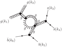
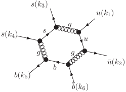
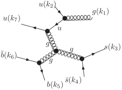
In the next step we use the optimising code generator haggies [157] for generating efficient Fortran 90 code for each diagram. The program haggies combines a multivariate Horner scheme [158] and common coefficient extraction [159] with common subexpression elimination and a linear search strategy for variable allocation [160]. Its built in type checker allows one to build up expressions from different built-in and derived data types. The combination of these strategies optimises an expression with respect to the number of multiplications and function calls required for its evaluation. As an example, we consider the hexagon diagram in Figure 4: the Form output consists of 535 terms for one specific helicity amplitude, requiring 1100 multiplications for its evaluation. The program generated by haggies evaluates the same expression using 585 multiplications, saving roughly fifty percent of the required operations. Similarly, we process the sum of the 64 tree diagrams contributing to $qg\rightarrow s\bar{s}b\bar{b}q$ (See Fig. 4, right). One of the non-vanishing helicity amplitudes would require 12,279 multiplications and 5,128 additions before optimisation, whereas haggies produces a program that evaluates the result with only 2,166 multiplications and 687 additions, saving more than 80% of all arithmetic operations.

The program haggies works independent from the input and output language and is very flexible in the output format. Its design incorporates the possibility of writing code for object oriented programming languages, even if they do not support operator overloading. The program is therefore well suited for many problems both within and outside high energy physics. It is publicly available under http://www.nikhef.nl/~thomasr/download.php .

In the code generated by golem-2.0, the one-loop integrals are evaluated by the golem95 library. Its internal, recursive structure uses a cache for storing function evaluations which are required in different form factors belonging to the same diagram topology. We improved the performance of the numerical evaluation of the one-loop amplitude further by relating diagrams of which the loop propagators are contained in the set of loop propagators of another diagram. The form factors of the most difficult diagram of one topology can be reused for all pinched diagrams of the same topology by using the internal cache of golem95.

Besides the numerical code, the package is also capable of producing a description of the process in LaTeX including all contributing Feynman diagrams drawn with AxoDraw [161] combined with an implementation of the layout algorithm proposed in [162] (See Figure 4).

Figure 4: Three diagrams contributing to different subprocesses of $pp\rightarrow s\bar{s}b\bar{b}$ at NLO in QCD. The diagrams have been drawn automatically by golem-2.0 using LaTeX and AxoDraw [161].

We also plan to provide an interface to OPP like tensor reduction algorithms [91, 103] where our program provides the numerator function $N(q,\tilde{q}^{2})$ of diagrams or subamplitudes. Since our approach treats the numerator $n$-dimensional it provides the full $\tilde{q}^{2}$ dependence which can be used for the reconstruction of the rational term $R_{2}$.

5.4 The quark induced case of $pp\rightarrow b\bar{b}b\bar{b}$

For Higgs searches in many models beyond the Standard Model (BSM), processes with high multiplicities of $b$-quarks in the final state become relevant. For example, in a large part of the parameter space of the Minimal Supersymmetric Standard Model (MSSM), the light Higgs boson decays predominantly into $b\bar{b}$ pairs. This opens up the possibility to measure the $hhH$ coupling at the LHC through the process $gg\rightarrow H\rightarrow hh\rightarrow b\bar{b}b\bar{b}$. Experimental studies show, however, that such a measurement would be extremely difficult, primarily due to the overwhelming QCD background [163]. Another example where the $b\bar{b}b\bar{b}$ final state becomes important are hidden valley models where the decay of exotic hadrons leads to high multiplicities of $b$-quark. The precise knowledge of the $b\bar{b}b\bar{b}$ final state within the Standard Model is therefore an important factor for the success of these measurements. The calculation of the NLO corrections in $\alpha_{s}$ reduces the scale dependence of the prediction and therefore greatly improves the precision of this prediction. Here, we present the calculation of $q\bar{q}\rightarrow b\bar{b}b\bar{b}$ with $q\in\{u,d,s,c\}$, which is a subprocess of the reaction $pp\rightarrow b\bar{b}b\bar{b}$.

For the calculation of the virtual part of the amplitude we have applied the setup as discussed in Section 5.3. We have confirmed it by an independent implementation based on FeynArts and FormCalc [148] and a symbolical reduction of the tensor integrals to scalar integrals using the formalism described in [146].

The real corrections and the Born level amplitude as well as the phase space integration of all parts have been computed with MadGraph, MadEvent [164, 165] and MadDipole [166] and independently using an adapted version of Whizard [167]. In both cases the infrared singularities are treated by the subtraction of Catani-Seymour dipoles [168] with the improvements suggested in [169].

For all parts of the calculation we have used two independent implementations. Additional checks such as the cancellation of the infrared divergences, the symmetries of the amplitude and the independence on the slicing parameter in the dipoles [169] have been performed in order to ensure the correctness of our results.

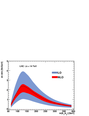
Figure 5 shows some results obtained for the LHC. We use a centre-of-mass energy of $\sqrt{s}=14\;\mathrm{TeV}$ and impose the following cuts on transverse momentum, rapidity and separation $\Delta R(b_{i},b_{j})=\sqrt{(\Delta\Phi_{ij})^{2}+(\Delta\eta_{ij})^{2}}$:

$$\begin{array}[]{rcl}p_{T}(b_{i})&>&30\;\mathrm{GeV}\\ |\eta(b_{i})|&<&2.5\\ \Delta R(b_{i},b_{j})&>&0.8\end{array}$$ (22)

Before cuts the $K_{T}$ algorithm [170] is applied to decide if the extra gluon in the real emission part of the process can be resolved. In the case of an unresolved gluon the momentum of the merged $b$-$g$-pair $p_{b_{i}}+p_{g}$ is used as the momentum of the $b$-jet. For the initial state we convolve with the $u$, $d$, $c$ and $s$-quark parton distribution functions of the CTEQ6M set [171] with two-loop running of $\alpha_{s}$ for the LO and the NLO part of the amplitude. We work in the limit $m_{b}=0$ and $m_{t}\rightarrow\infty$.

Figure 5: $pp(q\bar{q})\rightarrow b\bar{b}b\bar{b}+X$ at the LHC ($\sqrt{s}=14\;\mathrm{TeV}$). (left) The dependence of the cross-section on the renormalisation scale $\mu_{R}=x\mu_{0}$ at fixed value of the factorisation scale $\mu_{F}=100\;\mathrm{GeV}$. (right) Invariant mass ($m_{bb}$) distribution of the two leading $b$-jets (see text). The error bands are obtained from a variation of the renormalisation scale $\mu_{R}$ between $\mu_{0}/4$ and $2\mu_{0}$ with $\mu_{0}=\sqrt{\sum_{j}p_{T}^{2}(b_{j})}$. The dashed line shows the LO prediction for $\mu_{R}=\mu_{0}/2$.

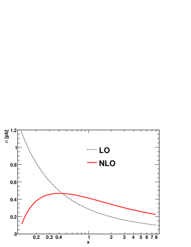
The left plot of Figure 5 shows the dependence of the total cross-section on the variation of the renormalisation scale while the factorisation scale is fixed at $\mu_{F}=100\;\mathrm{GeV}$. The NLO curve clearly shows the expected improvement of the scale dependence with a plateau region around a central value of $\mu_{0}/2$, where $\mu_{0}$ has been defined as $\mu_{0}=\sqrt{\sum_{j}p_{T}^{2}(b_{j})}$.

The right plot shows the invariant mass distribution of the leading two $b$-jets. The error bands obtained from a variation of the renormalisation scale in the interval $\mu_{0}/4<\mu_{R}<2\mu_{0}$ confirm the expected reduction of the renormalisation scale dependence.

CONCLUSIONS

We have reported on the recent progress of the Golem collaboration. We have started the development of a one-loop matrix element generator, called golem-2.0, based on the Feynman diagrammatic expansion of helicity amplitudes. This program has now been used to provide results for the order $\alpha_{s}$ virtual corrections of the amplitude $q\bar{q}\rightarrow b\bar{b}b\bar{b}$. We have combined this program with MadGraph/MadEvent and Whizard to obtain a complete next-to-leading order result for this process. The calculation of the remaining channels of $pp\rightarrow b\bar{b}b\bar{b}+X$ is in preparation.

The one-loop integral library golem95 has been extended to the case of massive loop propagators, which is necessary for many Standard Model processes. Moreover, together with the interface between golem-2.0 and Feynman rule generators such as FeynRules and LanHEP [172] we extended the applicability of our programs to BSM physics.

We focus on making the matrix element generator golem-2.0 publicly available as a plug-in into existing Monte Carlo event generators, using the Les Houches standard interface for one-loop programs [24], which should be accomplished within the next six months.

Our recent work demonstrates the potential of Feynman diagrams and the ability of our approach to handle processes with up to six external particles efficiently and in a highly automated manner and gives confidence that even higher particle multiplicities are within reach.

ACKNOWLEDGEMENTS

We would like to thank Thomas Gehrmann for interesting and useful discussions. T.B. thanks the University of Freiburg and Nikhef in Amsterdam, where parts of this work have been done, for their hospitality. T.B. is supported in parts by STFC, SUPA and the IPPP Durham. N.G. thanks the Universities Edinburgh, Freiburg and the IPPP in Durham for supporting various visits where work on the project was done. N.G. was supported by the Swiss National Science Foundation (SNF) under contract 200020-126691. G.H. and G.C. thank Nikhef for their hospitality. G.H. and M.R. are supported by STFC. N.K. thanks the Higher Education Funding Council for England (HEFCE) and the Science and Technology Facilities Council (STFC) for financial support under the SEPnet Initiative. IPPP Associates T.B. and N.K. thank the Institute for Particle Physics Phenomenology (IPPP) Durham for support. T.B. and N.K. thank the Galileo Galilei Institute for Theoretical Physics for the hospitality and the INFN for partial support during the completion of this work. T.R. thanks the University of Zürich and J.R. wants to thank the Aspen and Les Houches Centers of Physics for their hospitality. J.R. was partially supported by the Baden-Wuerttemberg Ministry of Science and Culture. Part of the computations were done on the ECDF cluster at the University of Edinburgh.

6 COMMON NTUPLE OUTPUT FORMAT FOR NLO CALCULATIONS

6.1 INTRODUCTION

Next-to-leading order (NLO) is the first order in perturbative QCD at which the normalizations, and in some cases, the shapes, of cross sections can be considered reliable. As has been reported in the proceedings of this workshop, there have been great advances in the NLO calculations of processes with multi-parton final states. From an experimental perspective, the ideal situation would be to have the NLO matrix elements interfaced to a parton shower Monte Carlo. So far this interface has been implemented only for a limited number of processes. It is important to devise techniques to allow this to be done for any NLO calculation, such as proposed in [173].

In the absence of a complete implementation of parton showering and hadronization for all NLO processes, it is still useful to examine the predictions from NLO calculations, at the parton level. A number of NLO authors have made public code available for their programs; for example, a large number of processes have been collected in MCFM [174]. There still remain, however, a number of important calculations for which no public code is available. In lieu of a public code, the authors can make parton 4-vector results from their calculations available. Information from any decay products (such as from W and Z bosons) can also be stored. Even for processes for which public code is available, it is still often useful to store the parton level event information. A convenient approach for this type of storage is ROOT [175]. ROOT allows for data compression, indexed access to specified events, immediate plotting of the variables, in addition to having wide acceptance in the experimental community. ROOT is one of the output options in MCFM, through the FROOT subroutine provided by Pavel Nadolsky. The format allows for the storage of all parton 4-vectors, the total event weight, the event weight by the initial state partons, and the event weights for the parton distribution error PDFs. The latter makes it easier to calculate the PDF uncertainty for any observables, at the expense of additional storage space.

In this short contribution, we would like to generalize the FROOT format, in order to provide a semi-official standard for NLO output. This is generally compatible with LHEF2.0 [176], but is much simplified, as less information is required. We also provide C++ classes to read and write the ntuple to disk, which shields the user from the technical details of the ROOT interface. At this workshop a standardized interface, the Binoth Les Houches Accord, between Monte Carlo and one-loop programs was developed [24]. However, this interface is not directly applicable to the NLO event storage problem that we are addressing here.

6.2 NTUPLE STRUCTURE

The ntuple structure in ROOT tree format is shown in Table 4. Branches are available for the following information:

• 4-vector information for the initial and final state partons;

• the momentum fractions $x_{1}$ and $x_{2}$ and PDG identification codes $id1$ and $id2$ of the incoming partons;

• factorization and renormalization scales;

• total event weight;

• there is provision for additional user-specified weights to be stored, for example for specific initial states;

• the event weights for a set of error PDFs;

• a unique event number, as well as event pointers are provided that allow relations between events to be stored.

Event relations (realized by pointers, see above) can be used, for example, to associate each generated real emission event with its counter-events resulting from Catani-Seymour dipole subtractions [168]. This allows the possibility of treating these events, which have potentially large cancellations between them, together, e.g. for more easily calculating the statistical error for the full sample, or any subset. Such relations could also prevent the inadvertent inclusion of an event without its corresponding counter-events, for instance due to incomplete reading of a ROOT tree.

All floating point variables are presently defined in double precision, since in most NLO calculations double precision is used per default. They could also be stored in single precision, which would save a factor of roughly two in disk space for the produced trees.

Table 4: Variables stored in the proposed common ROOT ntuple output.

ROOT Tree Branch	Description
Npart/I	number of partons (incoming and outgoing)
Px[Npart]/D	Px of partons
Py[Npart]/D	Py of partons
Pz[Npart]/D	Pz of partons
E[Npart]/D	E of partons
x1/D	Bjorken-x of incoming parton 1
x2/D	Bjorken-x of incoming parton 2
id1/I	PDG particle ID of incoming parton 1
id2/I	PDF particle ID of incoming parton 2
fac_scale/D	factorization scale
ren_scale/D	renormalization scale
weight/D	global event weight
Nuwgt/I	number of user weights
user_wgts[Nuwgt]/D	user event weights
evt_no/L	unique event number (identifier)
Nptr/I	number of event pointers
evt_pointers[Nptr]/L	event pointers (identifiers of related events)
Npdfs/I	number of PDF weights
pdf_wgts[Npdfs]/D	PDF weights

6.3 C++ IMPLEMENTATION

A set of C++ classes has been written for convenient input/output of the above described ROOT trees. Class LhaNLOEvent provides a container for the event information to be stored. The data members correspond to the Ntuple contents per event. Member functions are provided which set or get the event information. An example for storing the event information is shown below

LhaNLOEvent* evt = new LhaNLOEvent();
evt->addParticle(px1,py1,pz1,E1);
evt->setProcInfo(x1,id1,x2,id2);
evt->setRenScale(scale);
...

Another class LhaNLOTreeIO is responsible for writing the events into the ROOT tree and outputting the tree to disk. In addition to the event-wise information global data such as comments, cross sections etc can be written as well. An example is shown below:

LhaNLOTreeIO* writer = new LhaNLOTreeIO(); // create tree writer
writer->initWrite(’’test.root’’);
...
writer->writeComment(’’W+4 jets at NNLO’’); // write global comments
writer->writeComment(’’total cross section: XYZ+/-IJK fb’’);
...
writer->writeEvent(*evt); // write event to tree (in event loop)
...
writer->writeTree(); // write tree to disk

Similarly, a tree can be read back from disk:

LhaNLOTreeIO* reader = new LhaNLOTreeIO(); // init reader
ierr=reader->initRead("test.root");
if (!ierr) {
  for (int i=0; i< reader->getNumberofEvents();i++) {
    event->reset();
    ierr=reader->readEvent(i,*event);
    ...
  }
}

It is important to note that the details of the technical implementation of the tree and input/output using ROOT are shielded from the user, who interacts only with the LhaNLOEvent and LhaNLOTreeIO classes. The only requirement is that the ROOT libraries are provided when the program is compiled.

6.4 EXAMPLE

The aforementioned classes were interfaced with the C++ code for calculating the NLO cross section for the production of a top-antitop pair in association with one extra jet at the LHC from [177, 178]. Ntuples were produced for the leading-order (LO) contribution of the ttbar+jets process at a centre-of-mass energy of 10 TeV. The file size is of the order of 0.1 kilobytes/event (no PDF weights or event relations were used in this test, which would lead to bigger event sizes).

The results were compared in leading-order with MCFM, using ROOT trees produced with the FROOT package. MCFM was set to calculate the inclusive ttbar cross section at NLO. The comparison was made for the region of phase space where a third parton is produced in addition to the top-antitop pair (a cut $p_{T}>20\rm\ GeV$ was applied on this third parton). In this configuration the output of the two programs (TTJET LO vs MCFM NLO) should be identical, which is confirmed by Figure 6.

Figure 6: Comparison between the LO contribution to the ttbar+jet process, as calculated in [177, 178] (TTJET), and the NLO calculation of the total ttbar cross section as calculated in MCFM. A cut on the existance of a third parton with $p_{T}>20\rm\ GeV$ is applied in both cases, such that the predictions are comparable. Shown are the $p_{T}$ (top left), invariant mass (top right) and rapidity of the ttbar system (bottom left), as well as the dR between the top and the anti-top quark (bottom right).

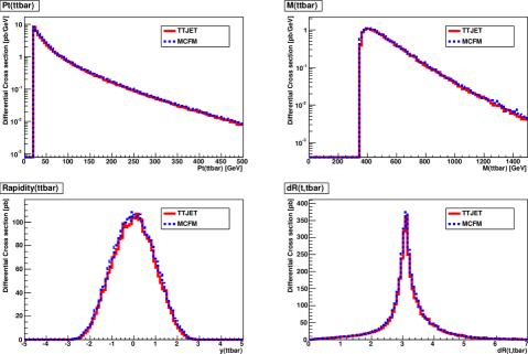
6.5 CONCLUSIONS

A common Ntuple output format for NLO cross section calculation codes based on ROOT trees has been proposed. It allows to make parton level 4-vector results of NLO calculations available even if no public code exists, and thus constitutes a valuable tool for exchange between theorists and experimentalists. The information provided in the Ntuples is essentially a sub-set of the Les Houches Event Format LHEF which is sufficient for applying cuts, plotting distributions etc. The interface can be easily adopted by many of the existing NLO codes.

In the future, a conversion tool between an LHE file and the Ntuple format described here could also be provided. Another possibility for an extension of the present proposal would be the storage of event weights for different renormalization and factorization scales, if the NLO programs were set up to provide this information. The source code is available from [179].

7 FIRST STEPS TOWARDS A DUALITY RELATION AT TWO LOOPS

7.1 INTRODUCTION

The duality method provides a method to numerically compute multi–leg one–loop cross sections in perturbative field theories by defining a relation between one–loop integrals and single phase–space integrals [180, 181, 93]. This is done by properly regularizing propagators by a complex Lorentz–covariant prescription, which is different from the customary $+i0$ prescription of the Feynman propagators. The duality method is valid for massless as well as for real and virtual massive propagators and can straightforwardly be applied not only for the evaluation of basic one–loop integrals but also for complete one–loop quantities such as Green’s functions and scattering amplitudes [93]. An extension to two–loop order is more involved and needs the treatment of occurring dependences on one of the two integration momenta in the modified $+i0$ description, which would lead to branch cuts in the complex energy plane. This extension is currently under investigation.

One motivation for deriving the duality relation is given by the fact that the computation of cross sections at next-to-leading order (NLO) requires the separate evaluation of real and virtual radiative corrections. Real (virtual) radiative corrections are given by multi–leg tree–level (one–loop) matrix elements to be integrated over the multi–particle phase space of the physical process. The loop–tree duality discussed here, as well as other methods that relate one–loop and phase–space integrals, have the attractive feature that they recast the virtual radiative corrections in a form that closely parallels the contribution of the real radiative corrections [182, 183, 180, 184, 185]. This close correspondence can help to directly combine real and virtual contributions to NLO cross sections. In particular, using the duality relation, one can apply mixed analytical and numerical techniques to the evaluation of the one–loop virtual contributions [180]. The infrared or ultraviolet divergent part of the corresponding dual integrals can be analytically evaluated in dimensional regularization. The finite part of the dual integrals can be computed numerically, together with the finite part of the real emission contribution. Partial results along these lines are presented in Refs. [180, 181] and further work is in progress.

7.2 THE DUALITY RELATION AT ONE–LOOP ORDER

Consider a generic one–loop integral over Feynman propagators, where $q_{i}=q+\sum_{k=1}^{i}p_{k}$ are the momenta of the internal lines, $q$ being the loop momentum, and $p_{i}$ ($\sum_{i=1}^{N}p_{i}=0$) the external (outgoing and clockwise ordered) momenta. The Feynman propagators have two poles in the complex plane of the loop energy $q_{0}$, the pole with positive (negative) energy being slightly displaced below (above) the real axis encoded by the additional $+i0$ term in the propagator. Using the Cauchy residue theorem in the complex $q_{0}$–plane, with the integration contour closed at $\infty$ in the lower half–plane, we obtain a sum over terms given by the integral evaluated at the poles with positive energy only. Hence a one–loop integral with $N$ internal propagators leads to $N$ contributions, one for each propagator for which the residue is taken. It can be shown that this residue is equivalent to cutting that line by including the corresponding on–shell propagator $\delta_{+}(q_{i}^{2})=\theta(q_{i}^{0})\delta(q_{i}^{2})$. The remaining propagators of the expression are shifted to

$$\left.\prod_{j\neq i}\,\frac{1}{q_{j}^{2}+i0}\,\right|_{q_{i}^{2}=-i0}=\prod_{j\neq i}\;\frac{1}{q_{j}^{2}-i0\,\eta(q_{j}-q_{i})}~{},$$ (23)

where $\eta$ is a future-like vector, i.e. a $d$-dimensional vector that can be either light-like $(\eta^{2}=0)$ or time-like $(\eta^{2}>0)$ with positive definite energy ($\eta_{0}\geq 0)$. The calculation of the residue at the pole of the $i^{\rm th}$ internal line modifies the $i0$ prescription of the propagators of the other internal lines of the loop. This modified regularization is named ‘dual’ $i0$ prescription, and the corresponding propagators are named ‘dual’ propagators. The dual prescription arises, because the original Feynman propagator $1/(q_{j}^{2}+i0)$ is evaluated at the complex value of the loop momentum $q$, which is determined by the location of the pole at $q_{i}^{2}+i0=0$. The presence of $\eta$ is a consequence of the fact that the residue at each of the poles is not a Lorentz–invariant quantity, since a given system of coordinates has to be specified to apply the residue theorem. Different choices of the future-like vector $\eta$ are equivalent to different choices of the coordinate system. The Lorentz–invariance of the loop integral is, however, recovered after summing over all the residues. For a one–loop integral, the term $\eta(q_{j}-q_{i})$ is always solely proportional to external momenta and hence defines a fixed pole in the $q_{0}$–plane.

Note that an extension to real and virtual massive propagators and full scattering amplitudes is straightforward and described in detail in Ref. [93].

7.3 FIRST STEPS TOWARDS TWO–LOOP ORDER

The fact that the term $\eta(q_{j}-q_{i})$ is proportional to external momenta only, is not valid anymore once going to the next loop order and considering a generic two–loop n–leg diagram. Taking the residues loop by loop for the two integration momenta introduces in some cases a dependence on one of the integration momenta in the difference of $\eta(q_{j}-q_{i})$. Hence we encounter not poles but rather branch cuts in the complex energy plane. To avoid this and more generally to avoid any dependence on integration momenta in the $\eta(q_{j}-q_{i})$–terms demands a reformulation of the propagators into another basis, which fulfills the required properties. First steps towards a two–loop expression obtained by such a transformation have been undertaken, while the full general two–loop expression is still under investigation.

ACKNOWLEDGEMENTS

This work was supported by the Ministerio de Ciencia e Innovación under Grant No. FPA2007-60323, CPAN (Grant No. CSD2007-00042), the Generalitat Valenciana under Grant No. PROMETEO/2008/069, and by the European Commission MRTN FLAVIAnet under Contract No. MRTN-CT-2006-035482 and by MRTN-CT-2006-035505 HEPTOOLS.

Part II NEW HIGH ORDER CALCULATIONS, WISHLIST

8 A NLO STUDY OF $t\bar{t}H\to t\bar{t}b\bar{b}$ SIGNAL VERSUS $t\bar{t}b\bar{b}$ BACKGROUND

8.1 Introduction

The associated production of a Higgs boson, with a $t\bar{t}$ pair, is going to play an important role for precision measurements of the Higgs boson Yukawa couplings at the LHC, especially in the range of masses $115~{}{\rm GeV}<M_{H}<140~{}{\rm GeV}$, where the Higgs decays predominantly in $b\bar{b}$ pairs. Whether or not it will also provide a discovery channel, very much depends on the ratio between this signal and the main QCD $t\bar{t}b\bar{b}$ background. A next-to-leading order (NLO) analysis of the inclusive $Ht\bar{t}$ production performed by two independent groups showed an increase of the leading order (LO) cross section by a factor of 1.2 at the central scale $\mu_{0}=m_{t}+m_{H}/2$ up to 1.4 at the threshold value $\mu=2\mu_{0}$, see [186, 187, 188, 189]. On the other hand, very recent calculations [190, 14, 16] showed a huge enhancement of the $t\bar{t}b\bar{b}$ background at NLO with a $K$ factor of the order of 1.77. Of course, much more detailed analyses are needed to establish the possibility of detecting the Higgs in this channel, based on distributions, rather than on a mere event counting, see e.g. [191]. To this aim, an accurate description of both signal and background is needed. A first step toward this, is the inclusion of the $H\to b\bar{b}$ decay directly into the NLO calculation of the signal. In this contribution, this is achieved by computing the factorisable QCD corrections to the Higgs signal $pp\to t\bar{t}H\to t\bar{t}b\bar{b}$ process. We consider higher order corrections to both production and decay of the Higgs boson, where the latter is modeled by the propagator with a fixed width which we computed with Hdecay [192].

NLO QCD corrections have been calculated with the help of the Helac-Nlo system. It consists of Helac-Phegas [193, 194, 195, 130], Helac-Dipoles [196], OneLOop [120] and Helac-1Loop [120], based on the OPP reduction technique [91] and the reduction code CutTools[103]. The Helac-Nlo system has also been used to compute the $pp\to t\bar{t}b\bar{b}$ background [16], allowing the comparisons presented in this work.

8.2 Results

For both signal and background, we consider the process $pp\rightarrow t\bar{t}b\bar{b}+X$ at the LHC, i.e. for $\sqrt{s}=14$ TeV. For the top-quark mass we take $m_{t}=172.6$ GeV, whereas all other QCD partons including b quarks are treated as massless. Higgs boson mass is set to $m_{H}$ = 130 GeV. Top quark mass renormalization is performed in the on-shell scheme, which fixes the renormalization of the top quark Yukawa coupling. As far as the b-quark Yukawa coupling is concerned, we renormalize it in the $\overline{MS}$ scheme, which makes it proportional to the $\overline{MS}$ mass of the b-quark, $\overline{m}_{b}(\mu)$. Finally, we transform this parameter into $\overline{m}_{b}(m_{H})$. While the difference is of higher order, we are motivated by the fact that we work in the narrow width approximation with $\Gamma_{H}$ calculated at $\mu=m_{H}$.

We consistently use the CTEQ6 set of parton distribution functions (PDFs) [171, 197] , i.e. we take CTEQ6L1 PDFs with a 1-loop running $\alpha_{s}$ in LO and CTEQ6M PDFs with a 2-loop running $\alpha_{s}$ in NLO, but the suppressed contribution from b quarks in the initial state has been neglected. The number of active flavors is $N_{F}=5$, and the respective QCD parameters are $\Lambda^{LO}_{5}=165$ MeV and $\Lambda^{MS}_{5}=226$ MeV. In the renormalization of the strong coupling constant, the top-quark loop in the gluon self-energy is subtracted at zero momentum. In this scheme the running of $\alpha_{s}$ is generated solely by the contributions of the light-quark and gluon loops. By default, we set the renormalization and factorization scales, $\mu_{R}$ and $\mu_{F}$, to the common value $\mu_{0}=m_{t}+m_{H}/2$ for the signal and $\mu_{0}=m_{t}$ for the background.

All final-state b quarks and gluons with pseudorapidity $|\eta|<5$ are recombined into jets with separation $\sqrt{\Delta\phi^{2}+\Delta y^{2}}>D=0.8$ in the rapidity– azimuthal-angle plane via the IR-safe $k_{T}$-algorithm  [198, 199, 200]. Moreover, we impose the following additional cuts on the transverse momenta and the rapidity of two recombined b-jets: $p_{T,b}>20$ GeV, $|y_{b}|<2.5$. The outgoing (anti)top quarks are neither affected by the jet algorithm nor by phase-space cuts.

Figure 7: Distribution in the transverse momentum (left panel) and in the rapidity (right panel) of the extra jet for $pp\to t\bar{t}H\rightarrow t\bar{t}b\bar{b}+X$ at the LHC.

Figure 8: Averaged distributions of $p_{T}(b)$ and $p_{T}(\bar{b})$ (left panel) and averaged distributions of $y(b)$ and $y(\bar{b})$ (right panel) for $pp\to t\bar{t}H\rightarrow t\bar{t}b\bar{b}+X$ at the LHC. The red solid line refers to NLO and the blue dotted line to LO result.

Figure 9: Averaged distributions of $p_{T}(t)$ and $p_{T}(\bar{t})$ (left panel) and averaged distributions of $y(t)$ and $y(\bar{t})$ (right panel) for $pp\to t\bar{t}H\rightarrow t\bar{t}b\bar{b}+X$ at the LHC. The red solid line refers to NLO and the blue dotted line to LO result.

Figure 10: Distribution of the invariant mass $m_{b\bar{b}}$ of the bottom-anti-bottom pair (a), distribution in the transverse momentum $p_{T_{b\bar{b}}}$ of the bottom-anti-bottom pair (b), distribution in the rapidity $y_{b\bar{b}}$ of the bottom-anti-bottom pair (c) and distribution in the transverse momentum $p_{T_{b}}$ of the bottom quark (d) for $pp\rightarrow t\bar{t}H\rightarrow t\bar{t}b\bar{b}+X$ and $pp\rightarrow t\bar{t}b\bar{b}+X$ at the LHC. The red solid line refers to the NLO QCD background, the blue dotted line to the LO QCD background, while the green dash-dotted and cyan dashed line to the NLO and LO signal, respectively.

Figure 11: Scale dependence of the total cross section for $pp\rightarrow t\bar{t}H\to t\bar{t}b\bar{b}+X$ at the LHC with $\mu_{R}=\mu_{F}=\xi\cdot\mu_{0}$ where $\mu_{0}=m_{t}+m_{H}/2$. The blue dotted curve corresponds to the LO, whereas the red solid one to the NLO order result.

Figure 12: Scale dependence of the total cross section for $pp\rightarrow t\bar{t}H\to t\bar{t}b\bar{b}+X$ at the LHC with $\mu_{R}=\mu_{F}=\xi\cdot\mu_{0}$ where $\mu_{0}=m_{t}+m_{H}/2$. The blue dotted curve corresponds to the LO, the red solid one to the NLO order result whereas the green dashed one to the NLO order result with a jet veto.

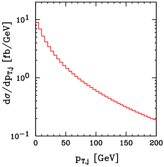
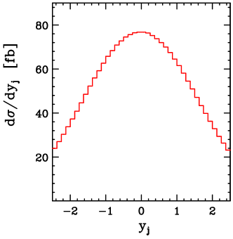
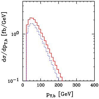
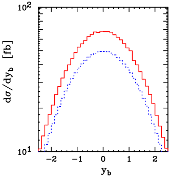
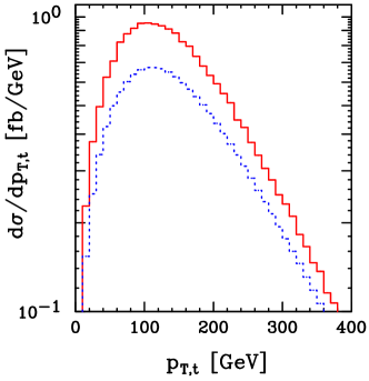
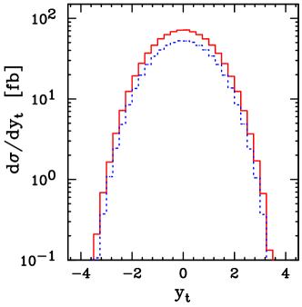
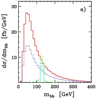
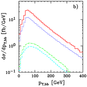
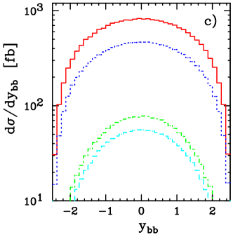
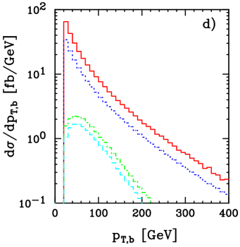
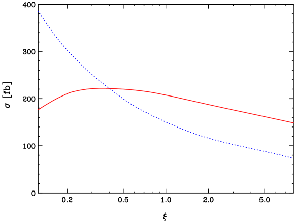
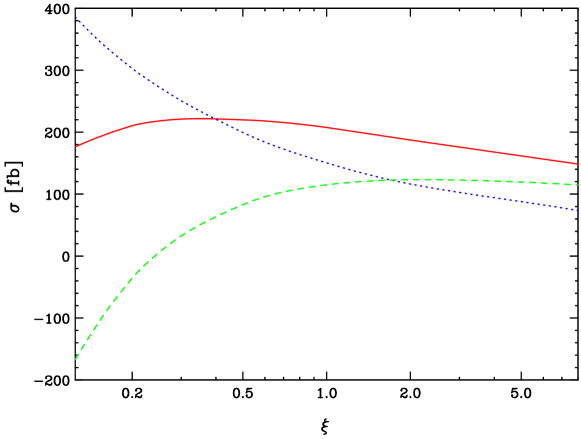
We first study the impact of the NLO corrections on the $pp\to t\bar{t}H\to t\bar{t}b\bar{b}$ signal. With the parameters and cuts specified above, the lowest order cross section is given by:

$$\sigma^{\rm S}_{\rm LO}=(150.375\pm 0.077)~{}{\rm fb}\,.$$ (24)

At the NLO we obtain

$$\sigma^{\rm S}_{\rm NLO}=(207.473\pm 0.232)~{}{\rm fb}\,~{}~{}~{}~{}{\rm for}~{}~{}\alpha_{\rm{max}}=0.01\,,$$ (25)

$$\sigma^{\rm S}_{\rm NLO}=(207.268\pm 0.150)~{}{\rm fb}\,~{}~{}~{}~{}{\rm for}~{}~{}\alpha_{\rm{max}}=1$$ (26)

which leave us with a $K$ factor $K=1.38$. We run our code with two different values of $\alpha_{max}$, which is a common modification of Catani-Seymour subtraction terms [168, 201] in the phase space region away from the singularity, see  [16] for details, to check the independence of the final result on this value. This has to be compared with a LO and NLO $t\bar{t}b\bar{b}$ background cross sections given by [16]:

$$\sigma^{\rm B}_{\rm LO} = (1489.2\pm 0.9)~{}{\rm fb}\,,$$ (27)

$$\sigma^{\rm B}_{\rm NLO}=(2636\pm 3)~{}{\rm fb}\,~{}~{}~{}~{}{\rm for}~{}~{}\alpha_{\rm{max}}=0.01\,,$$ (28)

$$\sigma^{\rm B}_{\rm NLO}=(2642\pm 3)~{}{\rm fb}\,~{}~{}~{}~{}{\rm for}~{}~{}\alpha_{\rm{max}}=1$$ (29)

again for two different values of $\alpha_{max}$ parameter. At $\mu_{0}=m_{t}$ we obtained the $K$ factor $K=1.77$.

The transverse momentum and rapidity distributions of the extra jet for the $pp\to t\bar{t}H\to t\bar{t}b\bar{b}$ process are presented in Fig. 7, from which it is evident, that most of the extra radiation is at low $p_{T}$ and in the central region, as expected. It is therefore tempting to study the effect of a jet veto on the $K$ factor for the signal process. With a jet veto of 50 GeV we obtain instead

$$\sigma^{\rm S}_{\rm NLO-veto}=(115.022\pm 0.233)~{}{\rm fb}\,~{}~{}~{}~{}{\rm for}~{}~{}\alpha_{\rm{max}}=0.01$$ (30)

$$\sigma^{\rm S}_{\rm NLO-veto}=(114.880\pm 0.152)~{}{\rm fb}\,~{}~{}~{}~{}{\rm for}~{}~{}\alpha_{\rm{max}}=1$$ (31)

giving $K=0.76$. We therefore conclude that NLO QCD corrections are reduced from +38% down to -24% when a jet veto of 50 GeV is applied on the additional jet. For comparison, we also quote here the result presented by Bredenstein, Denner, Dittmaier and Pozzorini in [14]. They find that a jet veto of 50 GeV reduces the NLO QCD corrections to the $t\bar{t}b\bar{b}$ background from +77% down to +20%, with respect to the tree level result.

The effect of the NLO corrections on the $p_{T}$ and rapidity distributions of bottoms and tops is shown in Fig. 8 and Fig. 9. The distributions are similar for particles and anti-particles, therefore the average is taken in the figures. The blue dotted curve corresponds to the LO, whereas the red solid one to the NLO order result.

As for the comparisons between signal and background, we present, in Fig. 10, a few histograms, namely the invariant mass, transverse momentum and rapidity of the two-$b$-jet system, as well as the transverse momentum of the single $b$-jet. In all figures the red solid line refers to the NLO QCD background, the blue dotted line to the LO QCD background, while the green dash-dotted and cyan dashed line to the NLO and LO signal, respectively. Apart from the invariant mass of the $b\bar{b}$ system and the $p_{T}$ spectrum of the $b$ quark, the shapes look very similar for signal and background.

Finally the scale dependence of the total cross section for $pp\rightarrow t\bar{t}H\to t\bar{t}b\bar{b}+X$ at the LHC is presented graphically in Fig. 11. The blue dotted curve corresponds to the LO, whereas the red solid one to the NLO order result. As expected, we observe a reduction of the scale uncertainty while going from LO to NLO. Varying the scale by a factor 2 changes the cross section by +33% and -23% in the LO case, while in the NLO case we have obtained a variation of the order +6% and -10%.

In Fig. 12 the impact of additional $p_{T}$ cut on the extra jet is shown. While for very small scales the scale dependence seems to have deteriorated, for the large one within the usual range, the variation remains more or less the same. Varying the scale up and down by a factor 2 changes the cross section by -28% and +7% in this case.

8.3 Conclusions

A NLO study of the $t\bar{t}H\to t\bar{t}b\bar{b}$ signal and the QCD $t\bar{t}b\bar{b}$ background reveals that the signal over background ratio R passes from R= 0.101 to R= 0.079, when inclusive NLO corrections are included. With a jet veto of 50 GeV, one obtains, instead, R= 0.064. A more detailed analysis is needed to study the effects of the jet veto procedure. However, our preliminary result shows that some tuning is necessary to maximize R. As for the distributions, the $p_{T}$ spectrum of the b quarks appears to be harder for the background than for the signal. This fact, together with an accurate reconstruction of the invariant $m_{b\bar{b}}$ mass, could be used as an extra handle to extract the Higgs signal.

Acknowledgments

This work was funded in part by the RTN European Programme MRTN-CT-2006-035505 HEPTOOLS - Tools and Precision Calculations for Physics Discoveries at Colliders. M.C. was supported by the Heisenberg Programme of the Deutsche Forschungsgemeinschaft. M.W. was supported by the Initiative and Networking Fund of the Helmholtz Association, contract HA-101 ("Physics at the Terascale"). M.V.G. and R.P. thank the financial support of the MEC project FPA2008-02984. M.V.G. was additionally supported by the INFN.

9 NLO QCD CORRECTIONS TO $\mathrm{\mathbf{t\bar{t}b\bar{b}}}$ PRODUCTION AT THE LHC

9.1 INTRODUCTION

The discovery of the Higgs boson and the measurement of its interactions with massive quarks and vector bosons represent a central goal of the Large Hadron Collider (LHC). In the light-Higgs scenario, $M_{\mathrm{H}}\mathrel{\raisebox{-3.00003pt}{$\stackrel{{\scriptstyle\displaystyle<}}{{\sim}}$}}130\,\mathrm{GeV}$, associated $\mathrm{t\bar{t}H}$ production provides the opportunity to observe the Higgs boson in the $\mathrm{H\to b\bar{b}}$ decay channel and to measure the top-quark Yukawa coupling. However, the extraction of the $\mathrm{t\bar{t}H(H\to b\bar{b})}$ signal from its large QCD backgrounds represents a serious challenge.

The selection strategies elaborated by ATLAS and CMS [202, 203, 204, 205, 206, 207, 208, 209] are based on the full reconstruction of the $\mathrm{t\bar{t}b\bar{b}}$ signature, starting from a final state with four $\mathrm{b}$ quarks and additional light jets. After imposing four $\mathrm{b}$ -taggings, a reconstruction of the top quarks is performed, which permits to identify two $\mathrm{b}$ quarks as top-decay products. The remaining two $\mathrm{b}$ quarks constitute a Higgs candidate, and their invariant-mass distribution is the relevant observable to find the Higgs signal. However, the presence of multiple $\mathrm{b}$ quarks and light jets in the final state represents a serious obstacle to the correct identification of the $\mathrm{b\bar{b}}$ Higgs candidates. Realistic simulations indicate that only about 1/3 of the selected $\mathrm{b}$ -quark pairs have correct combinatorics, while the other Higgs candidates contain $\mathrm{b}$ jets from top decays or miss-tagged light jets. This so-called combinatorial background significantly dilutes the Higgs signal and increases its background contamination. The QCD processes $\mathrm{pp\to t\bar{t}b\bar{b}}$ and $\mathrm{t\bar{t}jj}$ are the main background components. The latest ATLAS and CMS studies [205, 209], for $30\,\mathrm{fb}^{-1}$ and $60\,\mathrm{fb}^{-1}$, respectively, anticipate a statistical significance around $2\sigma$ (ignoring systematic uncertainties) and a fairly low signal-to-background ratio of order 1/10. This calls for better than 10% precision in the background description, a very demanding requirement both from the experimental and theoretical point of view.

More recently, an alternative strategy based on the selection of highly boosted Higgs bosons, which decay into “fat jets” containing two b quarks, has opened new and very promising perspectives [191]. This novel approach might enable a better background suppression and increase the signal-to-background ratio beyond $1/3$. Moreover, three $\mathrm{b}$ -taggings would be sufficient to strongly suppress the $\mathrm{t\bar{t}jj}$ contamination. In this case the background would be completely dominated by $\mathrm{t\bar{t}b\bar{b}}$ production.

The recent calculation of the NLO QCD corrections to the irreducible $\mathrm{t\bar{t}b\bar{b}}$ background [190, 14, 15, 16] constitutes another important step towards the observability of $\mathrm{t\bar{t}H(H\to b\bar{b})}$ at the LHC. These NLO predictions are mandatory in order to reduce the huge scale uncertainty of the lowest-order (LO) $\mathrm{t\bar{t}b\bar{b}}$ cross section, which can vary up to a factor four if the QCD scales are identified with different kinematic parameters [202, 203]. Previous results for five-particle processes that feature a signature similar to $\mathrm{t\bar{t}b\bar{b}}$ indicate that setting the renormalization and factorization scales equal to half the threshold energy, $\mu_{\mathrm{R,F}}=E_{\mathrm{thr}}/2$, is a reasonable scale choice. At this scale the NLO QCD corrections to $\mathrm{pp\to t\bar{t}H}$ ($K\simeq 1.2$) [186, 187, 188, 189], $\mathrm{pp\to t\bar{t}j}$ ($K\simeq$1.1) [177, 178], and $\mathrm{pp\to t\bar{t}Z}$ ($K\simeq 1.35$) [210], are fairly moderate. This motivated experimental groups to adopt the scale $\mu_{\mathrm{R,F}}=E_{\mathrm{thr}}/2=m_{\mathrm{t}}+m_{\mathrm{b\bar{b}}}/2$ for the LO simulation of the $\mathrm{t\bar{t}b\bar{b}}$ background [202, 203, 204, 205]. However, at this scale the NLO corrections to $\mathrm{pp\to t\bar{t}b\bar{b}}$ turn out to be close to a factor of two $(K\simeq 1.8)$ [14, 16]. This sizable NLO correction suggests the presence of large logarithms that tend to spoil the convergence of the perturbative expansion. This is mainly due to the fact that the scale $\mu_{\mathrm{R,F}}=E_{\mathrm{thr}}/2$ does not provide an adequate description of the QCD dynamics of $\mathrm{t\bar{t}b\bar{b}}$ production. To cure this problem we advocate the use of a new and more natural scale choice [15], which leads to a much smaller $K$ factor and also reduces the residual scale dependence at NLO. We then present a selection of the results of Ref. [15]. In particular we discuss the impact of a jet veto, as well as NLO effects on distributions that are relevant for the $\mathrm{t\bar{t}H}$ analysis, both within the traditional ATLAS/CMS approach and in the boosted-Higgs framework.

9.2 PREDICTIONS FOR THE LHC

We study the process $\mathrm{pp\to t\bar{t}b\bar{b}}+X$ at $\sqrt{s}=14\,\mathrm{TeV}$. For the top-quark mass, renormalized in the on-shell scheme, we take the numerical value $m_{\mathrm{t}}=172.6\,\mathrm{GeV}$ [211]. All other QCD partons, including b quarks, are treated as massless particles. Collinear final-state configurations are recombined into infrared-safe jets using the $k_{\mathrm{T}}$-algorithm of Ref. [170]. We recombine all final-state $\mathrm{b}$ quarks and gluons with pseudorapidity $|\eta|<5$ into jets with separation $\sqrt{\Delta\phi^{2}+\Delta y^{2}}>D=0.4$. Requiring two $\mathrm{b}$ jets, this also avoids collinear singularities resulting from massless $\mathrm{g\to b\bar{b}}$ splittings. After recombination, we impose the following cuts on the transverse momenta and rapidities of the $\mathrm{b}$ jets:

$$p_{\mathrm{T,b}}>20\,\mathrm{GeV},\qquad|y_{\mathrm{b}}|<2.5.$$ (32)

Since top decays are not included in our calculation, we treat top quarks fully inclusively. We consistently use the CTEQ6 [171, 197] set of PDFs, i.e. we take CTEQ6L1 PDFs with a one-loop running $\alpha_{\mathrm{s}}$ in LO and CTEQ6M PDFs with a two-loop running $\alpha_{\mathrm{s}}$ in NLO, but neglect the suppressed contributions from b quarks in the initial state. The number of active flavours is $N_{\mathrm{F}}=5$, and the respective QCD parameters are $\Lambda_{5}^{\mathrm{LO}}=165\,\mathrm{MeV}$ and $\Lambda_{5}^{\overline{\mathrm{MS}}}=226\,\mathrm{MeV}$. In the renormalization of $\alpha_{\mathrm{s}}$ the top-quark loop in the gluon self-energy is subtracted at zero momentum. In this scheme, the running of $\alpha_{\mathrm{s}}$ is generated solely by the contributions of the light-quark and gluon loops.

In all recent ATLAS studies of $\mathrm{t\bar{t}H(H\to b\bar{b})}$ [202, 203, 204, 205] the signal and its $\mathrm{t\bar{t}b\bar{b}}$ background are simulated by setting the renormalization and factorization scales equal to half the threshold energy, $E_{\mathrm{thr}}=2m_{\mathrm{t}}+m_{\mathrm{b\bar{b}}}$. Being proportional to $\alpha^{4}_{\mathrm{s}}$, these LO predictions are extremely sensitive to the scale choice, and in Refs. [14, 16] it was found that at $\mu_{\mathrm{R,F}}=E_{\mathrm{thr}}/2$ the NLO corrections to $\mathrm{pp\to t\bar{t}b\bar{b}}$ are close to a factor of two. This enhancement is due to the fact that $\mathrm{pp\to t\bar{t}b\bar{b}}$ is a multi-scale process involving various scales well below $E_{\mathrm{thr}}/2$. While $m_{\mathrm{t}}$ sets a clear scale for the couplings to the top quarks, the inspection of differential distributions reveals that the cross section is saturated by $\mathrm{b}$ quarks with $p_{\mathrm{T,b}}\ll m_{\mathrm{t}}$ (see Fig. 13). In order to avoid large logarithms due to these different scales we advocate the use of the dynamical scale

$$\mu^{2}_{\mathrm{R}}=\mu^{2}_{\mathrm{F}}=m_{\mathrm{t}}\sqrt{p_{\mathrm{T,b}}p_{\mathrm{T,\bar{b}}}}.$$ (33)

As we will see from the reduction of the $K$ factor and the scale uncertainties, the scale choice (33) significantly improves the convergence of the perturbative expansion as compared to Refs. [14, 16]. In Sections 9.2.1 and 9.2.2 we present NLO distributions obtained with standard ATLAS/CMS cuts and in the regime of highly boosted $\mathrm{b\bar{b}}$ pairs, respectively.

9.2.1 The regime of high $\mathrm{\mathbf{b\bar{b}}}$ invariant mass

Here, after imposing the standard cuts (32), we select the kinematic region $m_{\mathrm{b\bar{b}}}>100\,\mathrm{GeV}$, which is relevant for standard ATLAS/CMS studies of $\mathrm{t\bar{t}H(H\to b\bar{b})}$. At the scale (33) we obtain the integrated cross sections $\sigma_{\mathrm{LO}}=786.3(2)\,\mathrm{fb}$ and $\sigma_{\mathrm{NLO}}=978(3)\,\mathrm{fb}$, corresponding to a $K$ factor of $1.24$. Factor-two scale variations shift the LO and NLO predictions by 78% and 21%, respectively. This is a significant improvement with respect to the scale choice of Ref. [14], which yields $K=1.77$ and 33% NLO scale uncertainty. The NLO cross section at the scale (33) is a factor $2.18$ larger as compared to the LO prediction obtained with the ATLAS scale choice, $\left.\sigma_{\mathrm{LO}}\right|_{\mu_{\mathrm{R,F}}=E_{\mathrm{thr}}/2}=448.7(1)\,\mathrm{fb}$.

Figure 13: Transverse-momentum of the harder ($\mathrm{b_{1}}$) and softer ($\mathrm{b_{2}}$) $\mathrm{b}$ jets and $m_{\mathrm{b\bar{b}}}$ distribution [15]: absolute LO and NLO predictions (left) and NLO $K$ factors (right) for $m_{\mathrm{b\bar{b}}}>100\,\mathrm{GeV}$. Uncertainty bands correspond to factor-two scale variations.

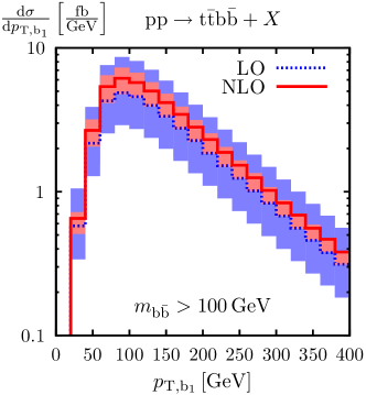
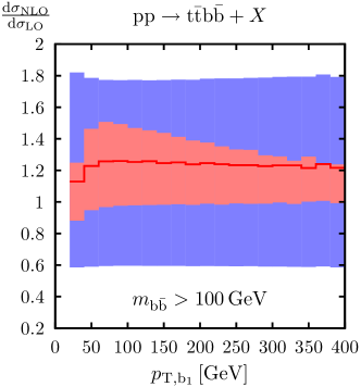
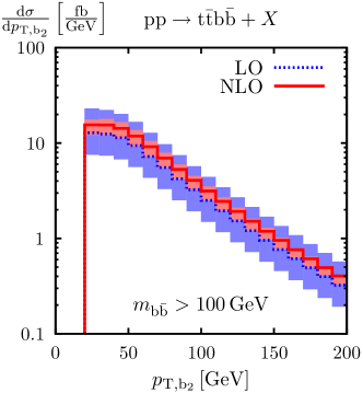
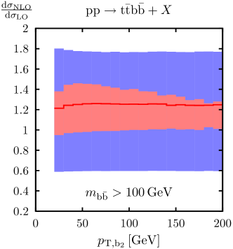
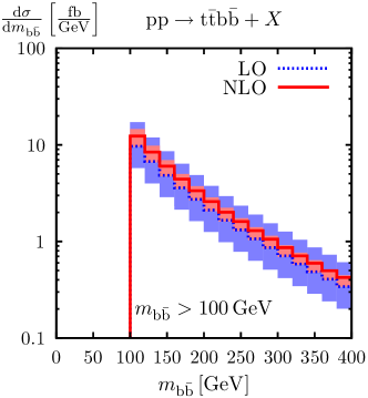
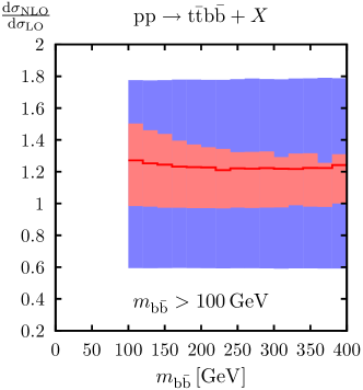
In Fig. 13 we present LO (blue) and NLO (red) results for various distributions. Besides absolute predictions (left column) we show results normalized to the LO distributions at the central scale (33) (right column). The bands correspond to factor-two variations of $\mu_{\mathrm{R,F}}$. The first two observables are the transverse momenta of the two $\mathrm{b}$ jets ordered in $p_{\mathrm{T}}$. While the softer $\mathrm{b}$ jet ($p_{\mathrm{T,b_{2}}}$) tends to saturate the lower bound of $20\,\mathrm{GeV}$, the harder ($p_{\mathrm{T,b_{1}}}$) behaves rather differently. Its distribution has a maximum around $100\,\mathrm{GeV}$ and a tail that extends up to fairly high transverse momenta. These shapes suggest that one of the two quarks is often emitted from initial-state gluons, while the other one participates in the hard scattering. In contrast, none of the $\mathrm{b}$ quarks resulting from $\mathrm{t\bar{t}H}$ originates from initial-state radiation. This feature renders the cross section quite sensitive to $p_{\mathrm{T,b}}$ and might be exploited to improve the separation of the $\mathrm{t\bar{t}H}$ signal. The dynamical scale (33) accounts for the different kinematics of the two $\mathrm{b}$ jets and the extension of their transverse momenta over a wide $p_{\mathrm{T}}$ range. The goodness of this choice is confirmed by the stability of the $K$ factor over the entire $p_{\mathrm{T}}$ spectrum. A similarly stable behaviour is observed for the $m_{\mathrm{b\bar{b}}}$ distribution in Fig. 13, where $1.21<K(m_{\mathrm{b\bar{b}}})<1.27$, as well as for various other distributions [15].

Figure 14: Dependence of the $\mathrm{pp\to t\bar{t}b\bar{b}}+X$ cross section on a jet veto ($p_{\mathrm{T,jet}}<p_{\mathrm{jet,veto}}$) [15]: absolute LO and NLO predictions (left) and NLO $K$ factor (right) for $m_{\mathrm{b\bar{b}}}>100\,\mathrm{GeV}$. The bands correspond to factor-two scale variations.

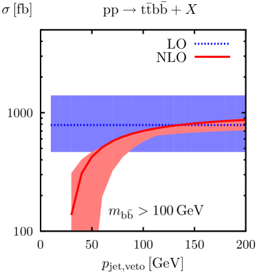
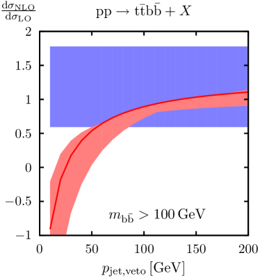
In Fig. 14 we study the potential of a jet veto ($p_{\mathrm{T,jet}}<p_{\mathrm{jet,veto}}$) to suppress the large $\mathrm{t\bar{t}b\bar{b}}$ background. The integrated cross section is plotted versus $p_{\mathrm{jet,veto}}$, and since jet radiation takes place only at NLO, the LO result is constant. The NLO curve shows that a sizable reduction of the cross section requires a jet veto well below $200\,\mathrm{GeV}$. For $p_{\mathrm{jet,veto}}=150,100$, and $50\,\mathrm{GeV}$, the $K$ factor is reduced to $1.03$, $0.89$, and $0.54$, respectively. However, there is a trade-off between suppressing the NLO cross section and increasing its perturbative uncertainty. The jet veto tends to destroy the cancellation between infrared logarithms of virtual and real origin and its effect grows as $-\alpha_{\mathrm{s}}^{5}\ln^{2}(E_{\mathrm{thr}}/p_{\mathrm{jet,veto}})$ when $p_{\mathrm{jet,veto}}$ becomes small. Since they are accompanied by an $\alpha_{\mathrm{s}}^{5}$ coefficient, these logarithms can give rise to huge scale uncertainties already for moderate values of $p_{\mathrm{jet,veto}}$. This is reflected by the dramatic amplification of the uncertainty band in Fig. 14. Around $p_{\mathrm{jet,veto}}=50\,\mathrm{GeV}$ the NLO band enters the pathologic regime of negative cross sections, and perturbative predictions become completely unreliable. Jet-veto values around $100\,\mathrm{GeV}$ provide a good compromise: the reduction of the $K$ factor is already significant ($K\simeq 0.89$) and the NLO scale uncertainty (19%) is at the same level as for the total cross section (21%).

9.2.2 The regime of highly boosted $\mathrm{\mathbf{b\bar{b}}}$ pairs

Here, after imposing the standard cuts (32), we select highly boosted $\mathrm{b\bar{b}}$ pairs with $p_{\mathrm{T,b\bar{b}}}>200\,\mathrm{GeV}$. This permits to increase the separation between the Higgs signal and its $\mathrm{t\bar{t}b\bar{b}}$ background [191]. Although we do not impose any cut on the $\mathrm{b\bar{b}}$ invariant mass, the cuts on $p_{\mathrm{T,b\bar{b}}}$, $p_{\mathrm{T,b}}$ and $p_{\mathrm{T,\bar{b}}}$, and the jet algorithm ($\Delta R_{\mathrm{b\bar{b}}}>0.4$), result into a lower bound $m_{\mathrm{b\bar{b}}}\mathrel{\raisebox{-3.00003pt}{$\stackrel{{\scriptstyle\displaystyle>}}{{\sim}}$}}25\,\mathrm{GeV}$ [15]. At the scale (33) we obtain the integrated cross sections $\sigma_{\mathrm{LO}}=451.8(2)\,\mathrm{fb}$ and $\sigma_{\mathrm{NLO}}=592(4)\,\mathrm{fb}$. As compared to the previous setup ($m_{\mathrm{b\bar{b}}}>100\,\mathrm{GeV}$) the absolute cross section is reduced by about $40\%$, the NLO correction is slightly increased ($K=1.31$), and the shifts induced by factor-two scale variations are almost identical (79% in LO and 22% in NLO). In presence of a jet veto of 100 GeV the $K$ factor and the NLO uncertainty amount to 0.84 and 33%, respectively.

Figure 15: Transverse-momentum of the harder ($\mathrm{b_{1}}$) and softer ($\mathrm{b_{2}}$) $\mathrm{b}$ jets and $m_{\mathrm{b\bar{b}}}$ distribution [15]: absolute LO and NLO predictions (left) and NLO $K$ factors (right) for $p_{\mathrm{T,b\bar{b}}}>200\,\mathrm{GeV}$. Uncertainty bands correspond to factor-two scale variations.

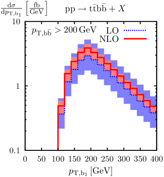
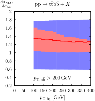
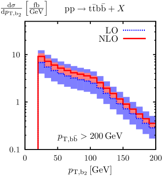
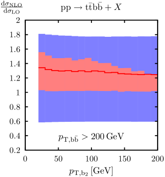
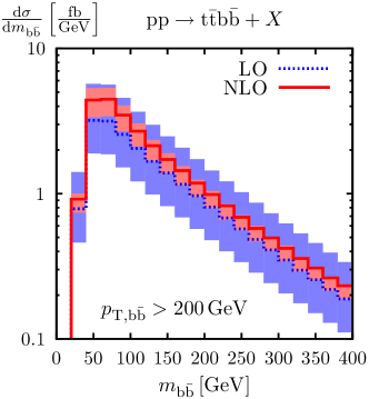
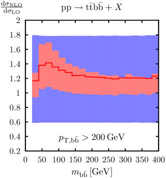
In Fig. 15 we present the distributions of the transverse momenta of the harder ($p_{\mathrm{T,b_{1}}}$) and softer ($p_{\mathrm{T,b_{2}}}$) $\mathrm{b}$ jets and the $\mathrm{b\bar{b}}$ invariant mass. As a consequence of the cut $p_{\mathrm{T,b\bar{b}}}>200\,\mathrm{GeV}$, the harder $\mathrm{b}$ jet is pushed to much higher $p_{\mathrm{T}}$ values as compared to Fig. 13: the maximum of its distribution is located around 200 GeV. In contrast, the softer $\mathrm{b}$ jet is much less sensitive to the $p_{\mathrm{T,b\bar{b}}}$ cut and is predominantly produced in the region $20\,\mathrm{GeV}<p_{\mathrm{T,b_{2}}}<100\,\mathrm{GeV}$. This different kinematic behaviour of the two $\mathrm{b}$ jets might be exploited to separate the $\mathrm{t\bar{t}b\bar{b}}$ background from the $\mathrm{t\bar{t}H}$ signal, where both $\mathrm{b}$ jets are produced by the Higgs boson and should thus have more similar $p_{\mathrm{T}}$-values. As a consequence of the dynamical scale choice, the NLO corrections feature a mild dependence on the $\mathrm{b}$-jet $p_{\mathrm{T}}$: the $K$ factor varies by about 10% within the plotted range.

The $\mathrm{b\bar{b}}$ invariant-mass distribution is displayed in the third row of Fig. 15. Its behaviour in the region $m_{\mathrm{b\bar{b}}}\mathrel{\raisebox{-3.00003pt}{$\stackrel{{\scriptstyle\displaystyle<}}{{\sim}}$}}50\,\mathrm{GeV}$ reflects the abovementioned effective bound. Near the physically interesting region of $m_{\mathrm{b\bar{b}}}\sim 100\,\mathrm{GeV}$ we observe that the NLO corrections induce an appreciable shape distortion of about 20%. Such an effect tends to mimic a Higgs signal and should be carefully taken into account in the $\mathrm{t\bar{t}H(H\to b\bar{b})}$ analysis.

CONCLUSIONS

The observation of the $\mathrm{t\bar{t}H(H\to b\bar{b})}$ signal at the LHC requires a very precise description of the $\mathrm{t\bar{t}b\bar{b}}$ irreducible background. The NLO QCD corrections reveal that the scale choice adopted in previous lowest-order simulations of $\mathrm{pp\to t\bar{t}b\bar{b}}$ does not account for the multi-scale character of this process and underestimates its cross section by a factor of two. We advocate the use of a new dynamical scale, which significantly reduces both the $K$ factor and the residual NLO scale uncertainty. In presence of standard ATLAS/CMS cuts NLO effects feature small kinematic dependence. But in the regime of highly boosted Higgs bosons we observe significant distortions in the shape of distributions. Studying a jet veto as a possible strategy to suppress the $\mathrm{t\bar{t}b\bar{b}}$ background, we find that jet-veto values well below 100 GeV lead to severe perturbative instabilities and should thus be avoided. Further results are presented in Ref. [15].

10 UNDERSTANDING SOFT AND COLLINEAR DIVERGENCES TO ALL ORDERS

10.1 Introduction

The ultimate goal of our efforts as practitioners of quantum field theory applied to high-energy physics is the calculation of the finite transition probabilities and cross sections that form the predictions to be tested at particle colliders. It would be nice if we had methods to compute directly these finite quantities, without having to deal with divergences in the intermediate stages of our calculations. Our tools are, however, imperfect: perturbative methods in quantum field theory typically start out by mishandling both very short and very long wavelength excitations, and one finds divergent results along the way, which need to be regularized, properly interpreted, and finally cancelled in order to obtain the finite predictions that we need. At the high-frequency end of the spectrum, this is achieved by renormalization of the parameters of the theory, a process that we understand well and that we can carry out explicitly at high perturbative orders. At the low-frequency end of the spectrum, the solution is provided in principle by the construction of properly defined, sufficiently inclusive observables, as characterized by the Kinoshita-Lee-Nauenberg thorem. The practical implementation of this theoretical insight has however proven challenging, especially in the context of confining non-abelian gauge theories like QCD. Indeed, while we do have all-order perturbative proofs of factorization theorems and of the exponentiation of infrared and collinear divergences, not much was known until recently concerning the detailed structure of the anomalous dimensions that govern infrared exponentiation; on the other hand, at finite orders, the task of building a fully general and efficient subtraction algorithm to compute infrared-safe cross sections at NNLO in perturbation theory has been pursued by several groups for many years, however complete results are available so far only for processes with no hadrons in the initial state.

There is thus much that we still need to understand concerning infrared and collinear singularities, and it is perhaps worth recalling that we have strong motivations, both of theoretical and phenomenological nature, to study the problem. At the simplest level, the all-order structure of singularities for scattering amplitudes provides ‘theoretical predictions’ for a subset of terms arising in finite-order calculations, and these can be used to test the results obtained order by order. Much more interestingly, in infrared-safe observables the cancellation of singularities leaves behind logarithms of ratios of kinematic invariants, and these finite contributions tend to dominate the cross sections in the vicinity of thresholds and in other situations where soft radiation is predominant. The way in which logarithms arise as finite remainders, after summing contributions from real emission and from virtual corrections, is easily visualized in dimensional regularization. Setting $d=4-2\epsilon$, with $\epsilon<0$ for infrared regularization, the structure of the cancellation is typically of the form

$$\qquad\underbrace{{\frac{1}{\epsilon}_{\,\,}}_{\,}}_{\rm virtual}\,\,\,\,+\,\underbrace{(Q^{2})^{\epsilon}\int_{0}^{m^{2}}\frac{dk^{2}}{(k^{2})^{1+\epsilon}}}_{\rm real}\,\,\qquad\quad\Longrightarrow\,\,\,\,\,\,\ln(m^{2}/Q^{2})\,,$$ (34)

where $m$ is some scale associated with the chosen observable, say a jet mass. It is clear that the coefficients of the logarithms are dictated by the coefficients of the singular contributions, much as renormalization group logarithms are dictated by ultraviolet poles.

This tight relationship between singularities and logarithmic enhancements underlies a host of phenomenological applications: since singularities exponentiate, so do logarithms, and, as a consequence, finite-order calculations can be used to perform all-order resummations. These resummations actually take place in two rather different contexts, and with rather different tools. On the one hand, for sufficiently inclusive observables, one can perform the real-virtual cancellation analytically, and provide all-order expressions for the observable, to some definite logarithmic accuracy (the current standard being NNLL). On the other hand, data analysis at present colliders requires predictions for exclusive final states, in order to match the kinematic cuts dictated by experimental needs: to this end, one must supplement fixed order calculations with parton shower event generators, and subsequently hadronization. Parton showers effectively resum the same collinear and infrared logarithms, but they do so without implementing real-virtual cancellations: rather, they impose cutoffs on real radiation, and they generate multiparticle final states by iteration, mimicking the pattern of exponentiation of singularities. It should be emphasized that the coefficients of the relevant logarithms are the same: parton showers perform the resummation with suitable approximations (typically leading logarithmic, with the inclusion of some NLL terms, and typically taking the large-$N_{c}$ limit, as well as performing some sort of angular averaging) which are necessary in order to turn the quantum-mechanical time evolution into a Markov chain with an iterative probabilistic interpretation. Improving our understanding of infrared and collinear singularities can be instrumental for both these applications: the analytic treatment of inclusive cross sections would be performed to a higher logarithmic accuracy, and extended to complex processes where more partons participate in the hard interaction. In these circumstances an accurate description requires taking full account of the interference between amplitudes of different colour flow. These colour correlations are encoded in the singularity structure of multi-leg amplitudes. At the same time, the approximations employed in the fully-exclusive parton shower approach could be put under better theoretical control. Present day patron showers assume independent emission from individual partons, and consequently fail to describe soft radiation at large angles with respect to the jets. Upon considering multi-jet cross sections, the independent-emission approximation becomes less reliable, since soft gluon radiation gets increasingly sensitive to the underlying colour flow. In conclusion, in order to achieve the necessary precision for the complex QCD processes that will be under study at LHC, accurate predictions would be required for complex multi-jet cross section. These will be achieved both by extending the analytic approach to inclusive cross sections, and by improving the treatment of parton showers. Understanding the singularity structure is the first step towards achieving these goals.

One should remember, finally, that studying soft and collinear radiation means probing the long-distance behavior of the theory, and thus it is of great interest also from a purely theoretical standpoint. All massless gauge theories, at the perturbative level, have a remarkably similar singularity structure, governed by a set of common anomalous dimensions: the most important differences arise from the different behavior of the running coupling in different theories. In conformal gauge theories, such as ${\cal N}=4$ Super Yang-Mills (SYM), the pattern of exponentiation of divergences is greatly simplified by the simplicity of the running coupling, and has been used as a guideline to study the exponentiation of finite contributions to scattering amplitudes [212]. In a confining theory like QCD, resummation displays the divergent behavior of the perturbative series, which can be used to gauge the weight of non-perturbative effects in the kinematic regions in which their importance is enhanced. Good control on the size and shape of these power-suppressed effects has been achieved for inclusive distributions in simple processes which are electroweak at tree level [213, 214]: one may now hope that this level of understanding can be reached also for general multi-jet cross-sections.

With these motivations, we present below some recent striking theoretical developments, implying that the structure of infrared and collinear divergences in massless gauge theories, for amplitudes with any number of colored partons, and to all orders in the $1/N_{c}$ expansion, is significantly simpler than previously expected. In Sect. 10.2 we present an expression organizing all divergences as the exponentiation of a simple sum over contributions from color dipoles, that was recently proposed in Refs. [215, 216, 217, 218], and that reproduces all known results of finite order perturbative calculations. In Sect. 10.3 we explain how possible corrections to the dipole formula are tightly constrained, and in fact forced to have a very specific functional dependence on kinematics, which correlates to their color structure. Whether these corrections do indeed arise, starting with three-loop, four-point amplitudes, is the subject of current studies.

10.2 The dipole formula

Our goal in this section is to illustrate the recent progress in our understanding of soft and collinear singularities. The main result is the establishment, to all orders in perturbation theory, and for any $N_{c}$, of a set of differential equations, which strongly constrain the soft anomalous dimensions for general multi-parton, fixed-angle amplitudes, in any massless gauge theory. These equations were derived from factorization, and by enforcing the invariance of soft gluon dynamics under the rescaling of hard parton momenta. The simplest solution to these constraints, which reproduces all known fixed-order perturbative results, is a compact expression, encoding a simple correlation of color and kinematic degrees of freedom, and taking the form of a sum over color dipoles. Below, we illustrate the structure of this ‘dipole formula’: for the arguments suggesting its validity, and for detailed derivations of the constraint equations, we refer the reader to Refs. [216, 217].

Let ${\cal M}\left(p_{i}/\mu,\alpha_{s}(\mu^{2}),\epsilon\right)$ be a renormalized scattering amplitude involving a fixed number $n$ of hard coloured partons carrying momenta $p_{i}$, $i=1\,\ldots\,n$, all lightlike, plus any number of additional non-coloured particles. The singularities of ${\cal M}$ depend on all the kinematic invariants that can be formed out of the hard parton momenta, $p_{i}\cdot p_{j}$, which are all assumed to be of the same parametric size, and all large compared to $\Lambda_{\rm QCD}^{2}$. Momentum conservation is not imposed between the coloured partons, allowing for any recoil momentum to be carried by non-coloured particles in both the initial and final states. As far as color is concerned, ${\cal M}$ should be thought of as a vector in the vector space spanned by the color tensors available for the given set of hard partons. Soft and collinear factorization properties guarantee that all singularities can be absorbed into an overall multiplicative factor $Z$, acting as a matrix in color space. One writes formally

$${\cal M}\left(p_{i}/\mu,\alpha_{s}(\mu^{2}),\epsilon\right)\,=\,Z\left(p_{i}/\mu_{f},\alpha_{s}(\mu_{f}^{2}),\epsilon\right)\,\,{\cal H}\left(p_{i}/\mu,\mu/\mu_{f},\alpha_{s}(\mu^{2}),\epsilon\right)\,,$$ (35)

where ${\cal H}$ is a vector in color space, which remains finite as $\epsilon\to 0$, and we have introduced a factorization scale $\mu_{f}$ to isolate the infrared momentum region (below we will set $\mu_{f}=\mu$ for simplicity). Note that $\mu_{f}$ is introduced in the context of dimensional regularization and not as an explicit cutoff.

The matrix $Z$, accounting for all soft and collinear singularities, can be written in exponential form, as a consequence of appropriate evolution equations derived from factorization. The simplest expression for the logarithm of $Z$, satisfying all available constraints, and reproducing all known finite-order results, is a sum over color dipoles. $Z$ is thus conjectured to take the form

$$Z\left(p_{i}/\mu,\alpha_{s}(\mu^{2}),\epsilon\right) = \exp\Bigg{\{}\int_{0}^{\mu^{2}}\frac{d\lambda^{2}}{\lambda^{2}}\Bigg{[}\frac{1}{8}\,\widehat{\gamma}_{K}\left(\alpha_{s}(\lambda^{2},\epsilon)\right)\,\sum_{i\neq j}\,\ln\left(\frac{2p_{i}\cdot p_{j}\,{\rm e}^{-{\rm i}\pi\phi_{ij}}}{{\lambda^{2}}}\right)\,\mathrm{T}_{i}\cdot\mathrm{T}_{j}\,$$ (36)

$$-\,\frac{1}{2}\,\sum_{i=1}^{n}\,\gamma_{J_{i}}\left(\alpha_{s}(\lambda^{2},\epsilon)\right)\Bigg{]}\Bigg{\}}\,.$$

Let us briefly explain the notations in Eq. (36), and then pause to illustrate its physical content. The color structure of $Z$ is encoded in the color generators ${\rm T}_{i}$ associated with each hard parton, which are linked in color dipoles by the products $\mathrm{T}_{i}\cdot\mathrm{T}_{j}\equiv\sum_{a}\mathrm{T}_{i}^{a}\cdot\mathrm{T}_{j}^{a}$. The matrices ${\rm T}^{a}$ depend on the identity of the hard parton: for a final-state quark or an initial-state antiquark they are just the generators of the fundamental representation, $T^{a}_{\alpha\beta}=t^{a}_{\alpha\beta}$; for a final-state antiquark or an initial-state quark, $T^{a}_{\alpha\beta}=-t^{a}_{\beta\alpha}$; for a gluon, $T^{a}_{bc}={\rm i}\,f_{cab}$. This ensures that color conservation is simply expressed by $\sum_{i=1}^{n}\mathrm{T}_{i}^{a}=0$. The phases $\phi_{ij}$ are introduced to display how the analytic properties of the amplitude change when the invariants $p_{i}\cdot p_{j}$ change from time-like to space-like: we define $p_{i}\cdot p_{j}=-\left|p_{i}\cdot p_{j}\right|\,{\rm e}^{-{\rm i}\pi\phi_{ij}}$, where $\lambda_{ij}=1$ if $i$ and $j$ are both initial-state partons or are both final–state partons, and $\lambda_{ij}=0$ otherwise.

All singularities in Eq. (36) are generated through the integration over the scale $\lambda^{2}$ of the $d$-dimensional running coupling $\alpha_{s}(\lambda^{2},\epsilon)$ [219, 220], and are governed by the finite anomalous dimensions $\widehat{\gamma}_{K}(\alpha_{s})$ and $\gamma_{J_{i}}(\alpha_{s})$, which can be characterized as follows. $\gamma_{J_{i}}(\alpha_{s})$ is simply the anomalous dimension of the field corresponding to hard parton $i$, and is responsible for single collinear poles arising from radiation forming the virtual jet associated with that parton; it depends on parton spin as well as color, and it is known to three loops for quarks and gluons. $\widehat{\gamma}_{K}(\alpha_{s})$, on the other hand, is simply related to the cusp anomalous dimension $\gamma_{K}^{(i)}(\alpha_{s})$ [221], for Wilson lines in the color representation of parton $i$: in deriving Eq. (36), we have assumed that the latter is proportional to all orders to the appropriate quadratic Casimir operator, according to $\gamma_{K}^{(i)}(\alpha_{s})=C_{i}\,\widehat{\gamma}_{K}(\alpha_{s})$, a fact which is established up to three loops; factoring out the quadratic Casimir operator $C_{i}$ is important in deriving Eq. (36) since it can be expressed as $C_{i}={\rm T}_{i}\cdot{\rm T}_{i}$. The cusp factor in Eq. (36) is responsible for all singularities associated with soft gluons, including double poles arising from the exchange of gluons that are both soft and collinear to some hard parton: these double poles arise from the integration over the scale $\lambda^{2}$, thanks to the explicit factor of $\log\lambda^{2}$.

The striking feature of Eq. (36) is that it correlates color and kinematic degrees of freedom, and it does so in an unexpectedly simple way. Indeed, correlations through dipoles only are what one expects, and finds, at one-loop order, where only one soft gluon can be exchanged, correlating at most two hard partons. Beyond first order, the rules of eikonal exponentiation, as well as expectations from the analysis of ordinary Feynman diagrams, suggest that at $g$ loops one should expect contributions from gluon webs linking up to $g+1$ hard partons, and thus correlating $g+1$ momenta $p_{i}$ and color generators $T_{i}$ (an example of such a web is shown in Fig. 16, for $g=3$). Multiparton correlations in the exponent of Eq. (36) were shown to vanish at two loops in Ref. [222, 223], and at three loops for diagrams involving matter fields in Ref [224]. Although they cannot as yet be completely ruled out at higher orders, the derivation of Eq. (36) shows that they are tightly constrained: they can only arise starting at three loops, from webs correlating at least four partons, such as the one shown in Fig. 16, and they must have a very restricted dependence on color and kinematics, as briely discussed in Sect. 10.3

There at least three further features of Eq. (36) that should be emphasized. The first point is to note that Eq. (36) represents a very smooth generalization of the situation arising in the large $N_{c}$ limit: at large $N_{c}$, only planar diagrams contribute, which forces soft gluons to be exchanged only between adjacent hard partons in the specific color ordering being considered. This forces the color structure to be in the form of a sum over adjacent color dipoles, to all orders in perturbation theory; this color structure is in fact trivial and reduces to a product of color singlet form factors [212, 225, 226]. Eq. (36) generalizes this in a natural way, by simply extending the range of the sum to cover all possible dipoles, including non-adjacent ones: an extension which is sufficient to make the color exchange non-trivial, but simple enough to be determined at one loop. The second observation stems from the fact that the correlated color and momentum structures appearing in the exponent of Eq. (36) are fixed at one loop: the only effect of radiative corrections is to build up the anomalous dimensions $\widehat{\gamma}_{K}(\alpha_{s})$ and $\gamma_{J_{i}}(\alpha_{s})$. The consequence of this is that there is no need to introduce a path ordering in Eq. (36), even though it is an expression arising from the solution of a matrix evolution equation. When working in a definite color basis in order to apply Eq. (36) to some specific problem, the diagonalization of the anomalous dimension matrix can be performed once and for all at the one loop level, after which further radiative corrections affect just the anomalous dimensions. This leads to the third and final observation: Eq. (36) appears to give greater weight and a more solid theoretical foundation to the idea of employing the cusp anomalous dimension (or rather its representation-independent counterpart $\widehat{\gamma}_{K}(\alpha_{s})$, which is conjectured to be universal) as an effective charge for soft and collinear gluon emission. This idea, brought forward in [227] as a tool to improve the logarithmic accuracy of parton showers, and subsequently developed in [228, 229], is generalized by Eq. (36) beyond planar configurations, and appears to apply to the full complexity of QCD color exchange.

10.3 Possible corrections to the dipole formula

Having described in detail the structure and implications of the dipole formula, we must also clearly indicate its limitations and describe the corrections that may still arise at high perturbative orders, escaping the various constraints that have established it as a credible all-order ansatz.

Figure 16: A three-loop gluon web connecting four hard partons. Such webs are the possible sources of the lowest order admissible violations of the dipole formula, since they may yield functions of the conformal cross ratios $\rho_{ijkl}$.

First of all, let’s emphasize again that the dipole formula arises as the simplest solution to a set of constraint equations. These equations are derived by requiring the cancellation of an anomaly due to cusp singularities in the invariance of light-like Wilson lines under rescalings of their velocity vectors. Since this rescaling invariance is not anomalous for Wilson lines off the light cone, the constraints do not apply to lines corresponding to massive partons. Indeed, an analysis of amplitudes involving massive partons has shown [230] that the dipole formula breaks down for amplitudes involving at least two massive partons, already at the two-loop level. At two-loops, in that case, three-parton correlations arise, parametrized by two functions which have now been computed analytically at two loops [231, 232], and which vanish parametrically as the fourth power of the parton mass.

In the case of massless partons, the constraints arising from factorization and rescaling invariance are much more powerful. While Eq. (36) is established as the simplest solution to the constraint equations, the same constraints also indicate that only two classes of corrections can arise at higher orders, going beyond dipole correlations. The first possible class of corrections arises if the cusp anomalous dimension $\gamma_{K}^{(i)}(\alpha_{s})$ turns out not be proportional to the quadratic Casimir $C_{i}$ to all orders. This can happen if $\gamma_{K}^{(i)}(\alpha_{s})$ receives contributions from higher-rank Casimir operators of the gauge group, as is the case, for example, for the four-loop QCD $\beta$ function. Contributions of this kind can, in principle, arise starting at four loops. Arguments were given in Ref. [217], based on symmetry and collinear consistency, suggesting that the contribution of the quartic Casimir operator is absent at four loops. On the other hand, studies of the cusp anomalous dimension at strong coupling, in the large-$N_{c}$ limit, in a special class of representations of the gauge group [233], suggest that higher-rank Casimir operators should contribute at sufficiently high orders. Whether these rather special color correlations ultimately play a role in the infrared structure of nonabelian gauge theories remains an interesting open problem.

The second class of potential corrections to the dipole formula arises from the fact that it is possible to respect the invariance under rescalings of hard parton momenta, simply by considering functions of ‘conformally invariant cross ratios’ of the form

$$\rho_{ijkl}\equiv\frac{p_{i}\cdot p_{j}\,p_{k}\cdot p_{l}}{p_{i}\cdot p_{k}\,p_{j}\cdot p_{l}}~{}.$$ (37)

Since these cross-ratios are by themselves rescaling invariant, they are not constrained by factorization. The rules of nonabelian exponentiation, however, imply that contributions of this kind must arise from gluon webs connecting directly at least four hard partons, which can only happen starting at three loops.

It should be emphasized, as noted in Ref. [217], that functions of conformal cross ratios are still strongly constrained by requiring consistency with known collinear limits, and by imposing Bose symmetry: these further constraints, for example, rule out functions linear in the logarithms of the cross ratios at three loops. A more systematic analysis of the constraints on the available functional forms was carried out in Ref. [234], where the limits on the possible degree of transcendentality of the functions involved were also taken into account. It turns out that functions satisfying all available constraints, and which might plausibly arise in the calculation of high-order Feynman diagrams, do exist, though they appear to form a very limited set. For example, considering polynomials in the logarithms of the conformal cross ratios, precisely one function survives the constraints at three loops. If however one allows for polylogarithmic dependence, further examples can be found. Whether indeed these ‘quadrupole’ corrections to the dipole formula do arise at three loops or beyond remains at the moment an open question.

Summarizing, a simple exponential all-order ansatz exists for the singularities of multi-parton amplitudes in massless gauge theories. It has a solid theoretical foundation, arising from soft-collinear factorization, and it is exact at two loops in the exponent. Furthermore, possible corrections at higher perturbative orders can arise from only two sources, and must have very restricted structures in both color and kinematics. The resulting picture is much simpler than might have been expected from previous analyses, and the remaining potential corrections are actively studied. We are on track to gain full control of the soft and collinear dynamics of massless gauge theories.

Acknowledgments

We are indebted to Thomas Binoth — who left us too soon — for drawing the attention of the Les Houches community to the work described in this contribution.

Work supported by by the European Community’s Marie Curie Research Training Network ‘Tools and Precision Calculations for Physics Discoveries at Colliders’ (‘HEPTOOLS’), under contract MRTN-CT-2006-035505.

11 LESSONS LEARNED FROM THE NNLO CALCULATION OF $e^{+}e^{-}\rightarrow 3\;\mbox{jets}$

11.1 INTRODUCTION

The process $e^{+}e^{-}\rightarrow 3\;\mbox{jets}$ is of particular interest for the measurement of the strong coupling $\alpha_{s}$. Three-jet events are well suited for this task because the leading term in a perturbative calculation of three-jet observables is already proportional to the strong coupling. For a precise extraction of the strong coupling one needs in addition to a precise measurement of three-jet observables in the experiment a precise prediction for this process from theory. This implies the calculation of higher order corrections. The process $e^{+}e^{-}\rightarrow 3\;\mbox{jets}$ has been been calculated recently at next-to-next-to-leading order (NNLO) in QCD [235, 236, 237, 238, 239, 240, 241]. This was a very challenging calculation and I will report on some of the complications which occurred during this computation. The lessons we learned from this process have implications to other processes which will be calculated at NNLO. The two processes closest related to $e^{+}e^{-}\rightarrow 3\;\mbox{jets}$ are $e^{-}p\rightarrow e^{-}+\;\mbox{2 jets}$ and $pp\rightarrow Z/W+\;\mbox{jet}$. These are obtained from crossing final and initial state particles. But also for processes like $pp\rightarrow\;\mbox{2 jets}$ and $pp\rightarrow t\bar{t}$ many techniques can be transferred.

11.2 THE CALCULATION

The master formula for the calculation of a three-jet observable at an electron-positron collider is

$$\langle{\cal O}\rangle = \frac{1}{8s}\sum\limits_{n\geq 3}\int d\phi_{n}{\cal O}_{n}\left(p_{1},...,p_{n},q_{1},q_{2}\right)\sum\limits_{helicity}\left|{\cal A}_{n}\right|^{2},$$ (38)

where $q_{1}$ and $q_{2}$ are the momenta of the initial-state particles and $1/(8s)$ corresponds to the flux factor and the average over the spins of the initial state particles. The observable has to be infrared safe, in particular this implies that in single and double unresolved limits we must have

$${\cal O}_{4}(p_{1},...,p_{4},q_{1},q_{2}) \rightarrow {\cal O}_{3}(p_{1}^{\prime},...,p_{3}^{\prime},q_{1},q_{2})\;\;\;\;\;\;\mbox{for single unresolved limits},$$

$${\cal O}_{5}(p_{1},...,p_{5},q_{1},q_{2}) \rightarrow {\cal O}_{3}(p_{1}^{\prime},...,p_{3}^{\prime},q_{1},q_{2})\;\;\;\;\;\;\mbox{for double unresolved limits}.$$ (39)

${\cal A}_{n}$ is the amplitude with $n$ final-state partons. At NNLO we need the following perturbative expansions of the amplitudes:

$$\left|{\cal A}_{3}\right|^{2}=\left.{\cal A}_{3}^{(0)}\right.^{\ast}{\cal A}_{3}^{(0)}+\left(\left.{\cal A}_{3}^{(0)}\right.^{\ast}{\cal A}_{3}^{(1)}+\left.{\cal A}_{3}^{(1)}\right.^{\ast}{\cal A}_{3}^{(0)}\right)+\left(\left.{\cal A}_{3}^{(0)}\right.^{\ast}{\cal A}_{3}^{(2)}+\left.{\cal A}_{3}^{(2)}\right.^{\ast}{\cal A}_{3}^{(0)}+\left.{\cal A}_{3}^{(1)}\right.^{\ast}{\cal A}_{3}^{(1)}\right),$$

$$\left|{\cal A}_{4}\right|^{2}=\left.{\cal A}_{4}^{(0)}\right.^{\ast}{\cal A}_{4}^{(0)}+\left(\left.{\cal A}_{4}^{(0)}\right.^{\ast}{\cal A}_{4}^{(1)}+\left.{\cal A}_{4}^{(1)}\right.^{\ast}{\cal A}_{4}^{(0)}\right),$$

$$\left|{\cal A}_{5}\right|^{2}=\left.{\cal A}_{5}^{(0)}\right.^{\ast}{\cal A}_{5}^{(0)}.$$ (40)

Here ${\cal A}_{n}^{(l)}$ denotes an amplitude with $n$ final-state partons and $l$ loops. We can rewrite symbolically the LO, NLO and NNLO contribution as

$$\langle{\cal O}\rangle^{LO} = \int{\cal O}_{3}\;d\sigma_{3}^{(0)},$$

$$\langle{\cal O}\rangle^{NLO} = \int{\cal O}_{4}\;d\sigma_{4}^{(0)}+\int{\cal O}_{3}\;d\sigma_{3}^{(1)},$$

$$\langle{\cal O}\rangle^{NNLO} = \int{\cal O}_{5}\;d\sigma_{5}^{(0)}+\int{\cal O}_{4}\;d\sigma_{4}^{(1)}+\int{\cal O}_{3}\;d\sigma_{3}^{(2)}.$$ (41)

The computation of the NNLO correction for the process $e^{+}e^{-}\rightarrow\mbox{3 jets}$ requires the knowledge of the amplitudes for the three-parton final state $e^{+}e^{-}\rightarrow\bar{q}qg$ up to two-loops [242, 243], the amplitudes of the four-parton final states $e^{+}e^{-}\rightarrow\bar{q}qgg$ and $e^{+}e^{-}\rightarrow\bar{q}q\bar{q}^{\prime}q^{\prime}$ up to one-loop [244, 77, 245, 246] and the five-parton final states $e^{+}e^{-}\rightarrow\bar{q}qggg$ and $e^{+}e^{-}\rightarrow\bar{q}q\bar{q}^{\prime}q^{\prime}g$ at tree level [247, 248, 249]. The most complicated amplitude is of course the two-loop amplitude. For the calculation of the two-loop amplitude special integration techniques have been invented [250, 251, 252, 253, 254, 255]. The analytic result can be expressed in terms of multiple polylogarithms, which in turn requires routines for the numerical evaluation of these functions [256, 257, 258].

11.3 SUBTRACTION AND SLICING

Is is well known that the individual pieces in the NLO and in the NNLO contribution of eq. (11.2) are infrared divergent. To render them finite, a mixture of subtraction and slicing is employed. The NNLO contribution is written as

$$\langle{\cal O}\rangle^{NNLO} = \int\left({\cal O}_{5}\;d\sigma_{5}^{(0)}-{\cal O}_{4}\circ d\alpha^{single}_{4}-{\cal O}_{3}\circ d\alpha^{(0,2)}_{3}\right)$$ (42)

$$+\int\left({\cal O}_{4}\;d\sigma_{4}^{(1)}+{\cal O}_{4}\circ d\alpha^{single}_{4}-{\cal O}_{3}\circ d\alpha^{(1,1)}_{3}\right)$$

$$+\int\left({\cal O}_{3}\;d\sigma_{3}^{(2)}+{\cal O}_{3}\circ d\alpha^{(0,2)}_{3}+{\cal O}_{3}\circ d\alpha^{(1,1)}_{3}\right).$$

$d\alpha^{single}_{4}$ is the NLO subtraction term for $4$-parton configurations, $d\alpha^{(0,2)}_{3}$ and $d\alpha^{(1,1)}_{3}$ are generic NNLO subtraction terms, which can be further decomposed into

$$d\alpha^{(0,2)}_{3} = d\alpha^{double}_{3}+d\alpha^{almost}_{3}+d\alpha^{soft}_{3}-d\alpha^{iterated}_{3},$$

$$d\alpha^{(1,1)}_{3} = d\alpha^{loop}_{3}+d\alpha^{product}_{3}-d\alpha^{almost}_{3}-d\alpha^{soft}_{3}+d\alpha^{iterated}_{3}.$$ (43)

In a hybrid scheme of subtraction and slicing the subtraction terms have to satisfy weaker conditions as compared to a strict subtraction scheme. It is just required that

(a) the explicit poles in the dimensional regularisation parameter $\varepsilon$ in the second line of eq. (42) cancel after integration over unresolved phase spaces for each point of the resolved phase space.

(b) the phase space singularities in the first and in the second line of eq. (42) cancel after azimuthal averaging has been performed.

Point (b) allows the determination of the subtraction terms from spin-averaged matrix elements. The subtraction terms can be found in [259, 260, 261]. The subtraction term $d\alpha^{(0,2)}_{3}$ without $d\alpha^{soft}_{3}$ would approximate all singularities except a soft single unresolved singularity. The subtraction term $d\alpha^{soft}_{3}$ takes care of this last piece [239, 262]. The azimuthal average is not performed in the Monte Carlo integration. Instead a slicing parameter $\eta$ is introduced to regulate the phase space singularities related to spin-dependent terms. It is important to note that there are no numerically large contributions proportional to a power of $\ln\eta$ which cancel between the 5-, 4- or 3-parton contributions. Each contribution itself is independent of $\eta$ in the limit $\eta\rightarrow 0$.

11.4 MONTE CARLO INTEGRATION

The integration over the phase space is performed numerically with Monte Carlo techniques. Efficiency of the Monte Carlo integration is an important issue, especially for the first moments of the event shape observables. Some of these moments receive sizable contributions from the close-to-two-jet region. In the 5-parton configuration this corresponds to (almost) three unresolved partons. The generation of the phase space is done sequentially, starting from a 2-parton configuration. In each step an additional particle is inserted. In going from $n$ partons to $n+1$ partons, the $n+1$-parton phase space is partitioned into different channels. Within one channel, the phase space is generated iteratively according to

$$d\phi_{n+1} = d\phi_{n}d\phi_{unresolved\;i,j,k}$$ (44)

The indices $i$, $j$ and $k$ indicate that the new particle $j$ is inserted between the hard radiators $i$ and $k$. For each channel we require that the product of invariants $s_{ij}s_{jk}$ is the smallest among all considered channels. For the unresolved phase space measure we have

$$d\phi_{unresolved\;i,j,k} = \frac{s_{ijk}}{32\pi^{3}}\int\limits_{0}^{1}dx_{1}\int\limits_{0}^{1}dx_{2}\int\limits_{0}^{2\pi}d\varphi\;\Theta(1-x_{1}-x_{2})$$ (45)

We are not interested in generating invariants smaller than $(\eta s)$, these configurations will be rejected by the slicing procedure. Instead we are interested in generating invariants with values larger than $(\eta s)$ with a distribution which mimics the one of a typical matrix element. We therefore generate the $(n+1)$-parton configuration from the $n$-parton configuration by using three random numbers $u_{1}$, $u_{2}$, $u_{3}$ uniformly distributed in $[0,1]$ and by setting

$$x_{1}=\eta_{PS}^{u_{1}},\;\;\;x_{2}=\eta_{PS}^{u_{2}}\;\;\;\varphi=2\pi u_{3}.$$ (46)

The phase space parameter $\eta_{PS}$ is an adjustable parameter of the order of the slicing parameter $\eta$. The invariants are defined as

$$s_{ij}=x_{1}s_{ijk},\;\;\;s_{jk}=x_{2}s_{ijk},\;\;\;s_{ik}=(1-x_{1}-x_{2})s_{ijk}.$$ (47)

From these invariants and the value of $\varphi$ we can reconstruct the four-momenta of the $(n+1)$-parton configuration [263]. The additional phase space weight due to the insertion of the $(n+1)$-th particle is

$$w = \frac{1}{16\pi^{2}}\frac{s_{ij}s_{jk}}{s_{ijk}}\ln^{2}\eta_{PS}.$$ (48)

Note that the phase space weight compensates the typical eikonal factor $s_{ijk}/(s_{ij}s_{jk})$ of a single emission. As mentioned above, the full phase space is constructed iteratively from these single emissions.

Part III OBSERVABLES

12 COMPARISON OF PREDICTIONS FOR INCLUSIVE $W$ + 3 JET PRODUCTION AT THE LHC BETWEEN BlackHat, Rocket AND Sherpa

12.1 Introduction

Next-to-leading order (NLO) calculations are the first order at which the normalization, and sometimes the shape, of perturbative calculations can be considered reliable. On the other hand, experimenters deal primarily with leading order (LO) calculations, especially in the context of parton-shower Monte Carlo programs. Given the better accuracy at fixed order in the coupling, the predictions at NLO should be used (in appropriate regions of phase space) as a benchmark for the various types of LO calculations. This way the LO Monte Carlo programs can be validated, tuned and/or improved before the actual comparison with data will be pursued.

Many of the interesting final states at the Tevatron and LHC involve the production of a $W$ boson and multiple jets. Recently the NLO calculation for the hadro-production of final states consisting of a $W$ boson and 3 jets has been completed by two groups, one retaining the full colour information [122, 17], the other using a leading-colour approximation [18, 26, 126]. This calculation provides, for the first time, a reliable prediction for $W$ + 3 jet production both at the Tevatron and at the LHC. Searches for new physics will of course benefit from these new achievements, since they allow for a more detailed understanding of one of the major backgrounds to beyond Standard Model signals.

At NLO, the dependence on the renormalization and factorization scales is greatly reduced from that at LO. It has been noted that the use of some scales in LO calculations for $W$ + 3 jets can result in significant shape differences with NLO calculations. Conversely, the use of other scales at LO can mimic the results obtained at NLO. In Ref. [17] it has been shown that the use of a scale ($H_{T}$) equal to the scalar sum of the missing transverse energy and the transverse energies of the lepton and all jets in the event reproduces the shape of the NLO calculation at LO for many relevant kinematic distributions of a typical $W$ + 3 jet analysis, i.e. search cuts are applied in favour of $W$ production in association with jets. Dynamically generated scales, such as obtained with either the MLM or CKKW procedures [129], are typically much smaller than $H_{T}$. They usually are identified by backward clustering procedures that locally analyze the relative transverse momenta (or similar quantities) of pairs of hard matrix-element partons. As well known in QCD, the scale of the coupling should be determined by the relative $p_{T}$ of a branching that occurred in the perturbative evolution. As for the case of optimal scale choices at LO, a similar improved agreement with NLO predictions can be achieved by combining these dynamical scale schemes with the necessary Sudakov rejection or reweighting of events that are described by tree-level matrix elements of higher order. Advantageously, these matching approaches are largely independent of the kinematical cuts applied. Nevertheless, it is interesting to try to understand why the two different procedures for setting the scales lead to similar results. Of course, an NLO prediction for $W$ + 3 jets provides a better description of the cross section and kinematics, but experimenters are mostly confined to the use of LO predictions, where the full event can be simulated.

Figure 17: Scale dependence of the $W^{+}$ + 3 jet inclusive production at the LHC (10 TeV) at LO and NLO. The lower panel displays the $K$-factor. The cuts used are given in Section 12.2 At NLO the leading-colour adjustment procedure has been applied.

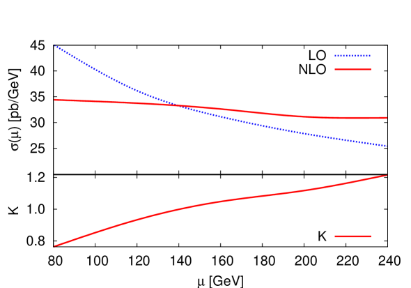
In Figure 17, we show the scale dependence for inclusive $W^{+}$ + 3 jet production at the LHC (10 TeV) at LO and NLO. The cross section at NLO has a smaller scale dependence than at LO as expected. The maximum cross section occurs near a scale of $m_{W}$, but is stable for a fairly wide range above that value. The LO cross section, of course, decreases monotonically with increasing scale, but the slope is less steep for larger scales. As can be seen in Figure 17 the choice of a renormalization/factorization scale such as $2\,m_{W}$ places the $W$ + 3 jet cross section in a region where the variation of the cross section with scale is reduced. (An examination of the scale dependence above and below the limits of this plot shows the usual parabolic scale dependence.) For typical values of $H_{T}$, of the order of $2\ldots 4\,m_{W}$, and cuts as given below, the LO and NLO inclusive cross sections will have a similar magnitude, i.e. the total $K$-factor (NLO/LO) tends to be close to unity ($1.0\ldots 1.25$) [28, 17].

12.2 Event generation parameters and description of the calculations

In this study we are comparing predictions for the production of $W^{+}$ bosons in association with 3 or more jets at LHC energies of 10 TeV, i.e. $PP\to e^{+}\nu_{e}$ + 3 jets at order $\alpha^{2}_{\mathrm{QED}}\alpha^{k}_{s}$ where $k\geq 3$. We consider the vector boson to decay leptonically into a pair of $e^{+}\nu_{e}$, hence all cross sections are given with the corresponding branching ratio taken into account. For our comparison, we apply cuts typical for signal studies. We require jets to have transverse momenta $p_{T,j}>30$ GeV and pseudo-rapidities $|\eta_{j}|<3$. Jets are defined according to the SISCone jet algorithm [265] with $\Delta R=\sqrt{\Delta\eta^{2}+\Delta\phi^{2}}=0.5$ and merging parameter $f=0.5$. For the leptonic sector, we cut on the lepton transverse momentum, $p_{T,e}>20$ GeV, the lepton pseudo-rapidity, $|\eta_{e}|<2.4$, the missing transverse energy, $\not{E}_{T}>15$ GeV, and the vector-boson transverse mass, $m_{T,W}=\sqrt{(|\vec{p}_{T,e}|+|\vec{p}_{T,\nu}|)^{2}-(\vec{p}_{T,e}+\vec{p}_{T,\nu})^{2}}>30$ GeV; we however do not impose lepton isolation cuts.

For all programs, we use the following parameters for the event generation: the processes $PP\to e^{+}\nu_{e}+n$ partons are calculated taking the quarks to be massless except for the top quark, which is not considered. For the value of $\alpha_{s}(m_{Z})$, we employ the fit result as given by the respective PDF. At NLO (LO) the $\alpha_{s}(\mu)$ values are evaluated from two-loop (one-loop) running. The $W$ boson mass is set to $m_{W}=80.419$ GeV, its couplings to fermions are calculated from $\alpha_{\mathrm{QED}}(m_{Z})=1/128.802$ and $\sin^{2}\theta_{\mathrm{W}}=0.230$; the CKM matrix is taken to be the identity matrix.

The different calculations used to obtain the $W^{+}$ + 3 jets predictions of this study have been accomplished in the following way:

• BlackHat+Sherpa [105, 122, 17]:
  We have used two programs for this comparison: the virtual matrix elements are evaluated by BlackHat [105]. The real part is computed within the Sherpa framework [132] using an automated Catani–Seymour dipole subtraction [168, 266, 267]. The phase-space integrations are entirely handled by Sherpa. All subleading colour contributions have been included in the calculation. The renormalization and factorization scales are commonly set to $\hat{H}_{T}=\sum_{\mathrm{partons}}E_{T,p}+E_{T,e}+E_{T,\nu}$, which is determined dynamically on an event by event basis. The sum runs over all partons in the event, regardless of whether they will pass the jet cuts. This prevents a jet-algorithm and cut dependency on the scale choice. At LO, summing over the transverse energies of the jets is equivalent to summing those of the partons.

• Rocket [109, 18, 26]:
  We closely follow Ref. [26] and perform calculations in the leading-colour approximation. The calculation relies heavily on the framework provided by MCFM [174] and uses one-loop amplitudes as calculated in Ref. [112]. We employ the Catani–Seymour dipole subtraction [168, 266] to compute the real emission corrections. The details of the implementation are given in [18, 126]. We use the leading-colour adjustment (aLC) procedure described in the latter paper to correct for deficiencies of the leading-colour approximation, to the extent possible. The renormalization and factorization scales are chosen to be equal and given by the transverse energy of the $W$ boson, which has been defined as $E_{T,W}=\sqrt{m^{2}_{W}+p^{2}_{T,W}}$. The top quark is assumed to be infinitely heavy; the running of the strong coupling therefore evaluated in the five-flavour scheme.

• Sherpa [132]:
  For the Sherpa event generation, we have used version 1.2.0 [268]. It incorporates a new strategy for merging tree-level higher-order matrix elements and parton showers, which we denote here as ME&TS (matrix-element & truncated-shower) merging [269, 270, 271]. This approach improves over the CKKW method owing to the incorporation of a consistent treatment of local scales that occur, on the one hand, in the matrix-element calculations and, on the other, in the parton showering. To ensure the strict ordering of the shower evolution, truncated shower algorithms are necessary for the ME&TS approach to work properly. As a result the systematic uncertainties of the ME&TS merging are greatly reduced with respect to CKKW. We have generated predictions from samples that merge matrix elements with up to $N^{\mathrm{max}}_{\mathrm{ME}}=2+3,2+4,2+5$ particles, i.e. $PP\to e^{+}\nu_{e}+n$ partons where $n=0,\ldots,N^{\mathrm{max}}_{\mathrm{ME}}-2$. Notice that $N^{\mathrm{max}}_{\mathrm{ME}}$ denotes the maximum number of final-state particles of the matrix elements. For the evaluation of the PDF scales, the default scheme of ME&TS has been employed. It is based on the identification of the most likely $2\to 2$ interaction that may lead to the actual $2\to 2+n$ matrix-element final state; the factorization scale is then chosen according to the kinematics of that $2\to 2$ core process [269]. Scales of the strong couplings are entirely determined by the ME&TS algorithm. The merging scale has been set to $Q_{\mathrm{cut}}=28$ GeV (to have it somewhat lower than the jet $p_{T}$ threshold). As for the comparison to the NLO results, the most relevant Sherpa prediction relies on the $N^{\mathrm{max}}_{\mathrm{ME}}=2+4$ merged sample, since it contains the real-emission matrix elements for 3 and 4 extra partons. For this case, we therefore have varied the default scales identified by the ME&TS algorithm by factors of $1/2$ and $2$. This leaves us with an estimate of the theoretical uncertainty of the ME&TS results.

We would like to stress the major differences between the different approaches: for the NLO case, the calculations only differ in their treatment of colour (full colour for BlackHat+Sherpa vs. leading colour for Rocket) and choice of scales ($\hat{H}_{T}$ for BlackHat+Sherpa vs. $E_{T,W}$ for Rocket). In the Sherpa case, it is evident that the virtual corrections to $W^{+}$ + 3 jets are not completely taken into account, they only enter in an approximate way through Sudakov form factor terms at leading-logarithmic accuracy. The scales cannot be set globally as in the NLO calculations, they have to be determined and set locally.

In addition to the predictions outlined above, we show LO $W^{+}$ + 3 jet parton-level results for two different choices of a common factorization and renormalization scale, $\mu=\mu_{\mathrm{F}}=\mu_{\mathrm{R}}$, defined by $\mu^{2}=\hat{H}^{2}_{T}$ and $\mu^{2}=E^{2}_{T,W}=m^{2}_{W}+p^{2}_{T,W}$. These results have been produced with the tree-level matrix-element generator Comix [272] by making use of the Sherpa event-generation framework.

In order to carry out a useful comparison, we tried to keep the generation parameters as common as possible among the different calculations. For example, in our main set of comparisons we use the same PDF, CTEQ6M with $\alpha_{s}(m_{Z})=0.118$, for both the NLO and LO predictions in order to separate any differences induced by PDFs from those resulting from the matrix elements. In all other cases the LO computations employ the CTEQ6L and CTEQ6L1 PDF sets with $\alpha_{s}(m_{Z})=0.118$ and $\alpha_{s}(m_{Z})=0.13$, respectively [171, 27].

12.3 Results of the comparison

Before we discuss differential distributions, we list in Table 5 the inclusive $e^{+}\nu_{e}$ + 3 jet cross sections for LHC energies of 10 TeV that we have obtained from all calculations outlined above. This gives us the possibility of rescaling the different results to the Rocket (aLC) NLO cross section, such that we can comment on shape differences in the differential distributions separately. The LO cross sections generated with Comix and given in Table 5 vary by more than a factor of 2 for different scale and PDF choices. At NLO this reduces to a 20% effect. This is still quite significant, but can be understood as a consequence of the different scale choices used in the NLO calculations: the $E_{T,W}$ choice of Rocket is found to yield average scales $\langle\mu_{\mathrm{F,R}}\rangle\approx 120$ GeV, whereas the $\hat{H}_{T}$ choice used by BlackHat+Sherpa generates considerably larger average values $\langle\mu_{\mathrm{F,R}}\rangle\approx 390$ GeV. This is more than a factor 3 higher. A change of 20% over such a large $\mu$ range seems reasonable, taking into account that the NLO cross section shown in Figure 17 already drops by about 10% between 120 GeV and 240 GeV. The variation among Sherpa’s ME&TS cross sections (about 75% at most) turns out to be smaller compared to what we find at LO. One should bear in mind that the two estimates are determined differently, for ME&TS, through varying the scales by constant factors and, for the LO case, by choosing different dynamic though global scales. The ME&TS cross sections decrease by an overall factor of 35% when including matrix elements with larger numbers of partons. The correction becomes weaker when adding in the 5-parton contributions (15% compared to 23% in the first step) indicating, as expected, a stabilization of the $W^{+}$ + $\geq 3$ jet cross sections of the ME&TS approach. The scales chosen by the ME&TS procedure reflect the local $p_{T}$ at each vertex of the hard interaction and will almost always be smaller than $H_{T}$. Nominally this results in a larger LO cross section and thus a smaller $K$-factor, but the Sudakov rejection applied with ME&TS reduces the resultant cross section to something smaller than that obtained at NLO (similar to that found at LO, cf. Table 5, $18.6$ pb vs. $17.3$ pb).

For the LO and ME&TS calculations, we also give results obtained from Run II $k_{T}$ jet finding using $D=0.5$ [170]. They are, in all cases, larger than their respective SISCone counterparts. Interestingly, the parton-shower corrections included by the ME&TS merging make the results from the two jet algorithms look very much alike, including the shapes of the differential distributions presented below.

Order	and  Specifics of calculation
LO	Comix	Comix	Comix
	$\mu=E_{T,W}$, CTEQ6L1	$\mu=E_{T,W}$, CTEQ6L	$\mu=H_{T}$, CTEQ6L
	37.1 pb	28.7 pb	17.3 pb
	43.8 pb  ($k_{T}$ jets)	33.8 pb  ($k_{T}$ jets)	20.6 pb  ($k_{T}$ jets)
NLO	Rocket (aLC)		BlackHat+Sherpa
	$\mu=E_{T,W}$, CTEQ6M		$\mu=\hat{H}_{T}$, CTEQ6M
	34.2 pb		28.6 pb
ME&TS	Sherpa	Sherpa	Sherpa
	$N^{\mathrm{max}}_{\mathrm{ME}}=2+3$, CTEQ6L	$N^{\mathrm{max}}_{\mathrm{ME}}=2+4$, CTEQ6L	$N^{\mathrm{max}}_{\mathrm{ME}}=2+5$, CTEQ6L
		20.1 pb  (CTEQ6M)
		14.3 pb  ($\mu=\mu^{\mathrm{ME\&TS}}\cdot 2$)
	24.3 pb	18.6 pb	15.8 pb
		24.7 pb  ($\mu=\mu^{\mathrm{ME\&TS}}/2$)
	24.4 pb  ($k_{T}$ jets)	18.8 pb  ($k_{T}$ jets)	16.0 pb  ($k_{T}$ jets)

Table 5: Inclusive $e^{+}\nu_{e}$ + 3 jet cross sections as obtained from the different calculations used in this study. For cuts, parameter settings and details of the calculations, cf. Section 12.2 If not stated otherwise, the SISCone jet algorithm [265] has been used to identify the jets. The $k_{T}$ Run II jet finder [170] has been applied for evaluating the cross sections labelled “$k_{T}$ jets”. The “aLC” label expresses the fact that we have used Rocket’s adjusted leading-colour result [126].

The main set of differential distributions of our comparative study is presented in Figures 18–21. For the comparisons with Rocket, we restrict ourselves to the distributions available in [126]. We also include new distributions only comparing BlackHat+Sherpa with the ME&TS approach. For the latter, we always show, as the default, the predictions obtained from the $N^{\mathrm{max}}_{\mathrm{ME}}=2+4$ merged sample using the CTEQ6M PDF. Although the cross sections differ by about 10%, see Table 5, we did not discover any significant shape alterations induced by switching to the CTEQ6L PDF set.

Figure 18: The transverse momentum distributions (left) and pseudo-rapidity distributions (right) of the three hardest jets in $W^{+}$ + $\geq 3$ jet production at the LHC. Predictions at NLO obtained from the BlackHat+Sherpa (black line) and Rocket (red line) codes are compared to LO results from Sherpa using the ME&TS merging. All curves have been rescaled to the Rocket NLO cross section of Table 5; BlackHat+Sherpa is used as the reference; cuts and parameters are detailed in Section 12.2

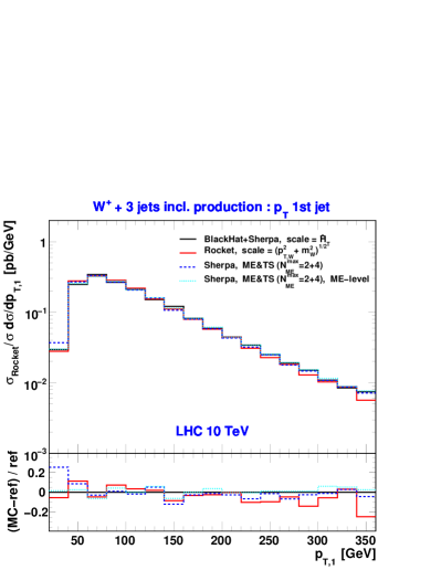
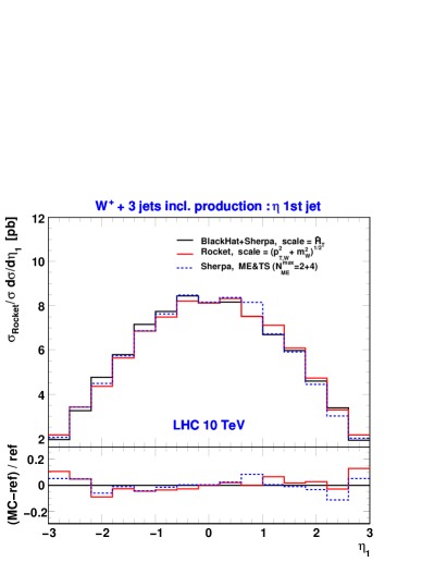
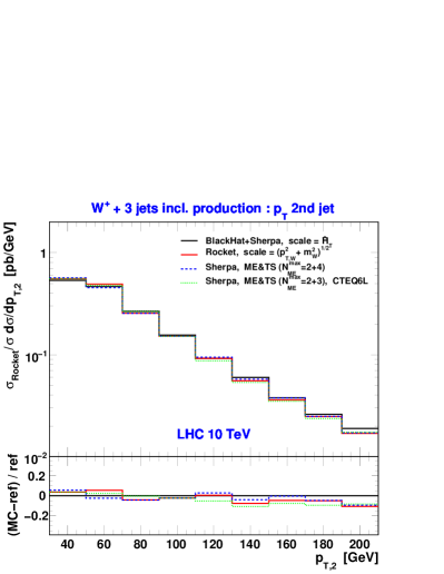
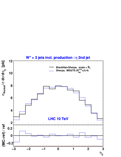
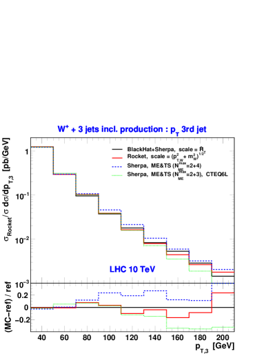
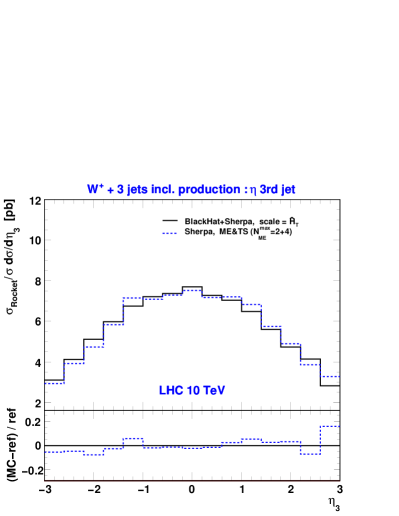
In Figure 18, we show the transverse momentum (left panels) and pseudo-rapidity (right panels) distributions for the three leading jets in $W^{+}$ + $\geq 3$ jet production. The two NLO predictions agree well with each other for all three $p_{T}$ and the leading-jet $\eta$ distributions, in spite of the different scales used for each calculation; this is another manifestation of the reduced scale dependence at NLO. Sherpa’s ME&TS $\eta$ curves are in good agreement with the NLO prediction(s). This level of agreement is also found for the first two hardest jets, for the third jet it depends more on the details of the Sherpa ME&TS generation. To this end we have added the predictions (dotted green lines) from the $N^{\mathrm{max}}_{\mathrm{ME}}=2+3$ merged sample in the second- and third-jet $p_{T}$ plots. As can be seen when omitting the contributions of the real-emission matrix elements with four extra partons, the corresponding transverse-momentum distributions fall below that of the NLO calculations, most noticeably for the third-jet $p_{T}$ spectrum. Once the matching is extended to $N^{\mathrm{max}}_{\mathrm{ME}}=2+4$, the Sherpa prediction for the second jet improves with respect to the NLO results, while the one for the third jet lies above those given at NLO.

Figure 19: $H_{T}$ and $H_{T,\mathrm{jets}}$ distributions in inclusive $W^{+}$ + 3 jet production at the LHC. NLO predictions obtained from BlackHat+Sherpa (black line) and Rocket (red line) are compared to LO results from Sherpa using the ME&TS merging. All curves have been rescaled to the Rocket NLO cross section of Table 5; the BlackHat+Sherpa prediction is used as the reference; cuts and parameters are detailed in Section 12.2

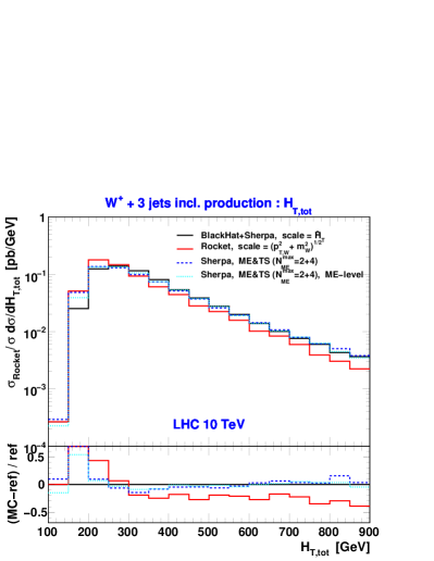
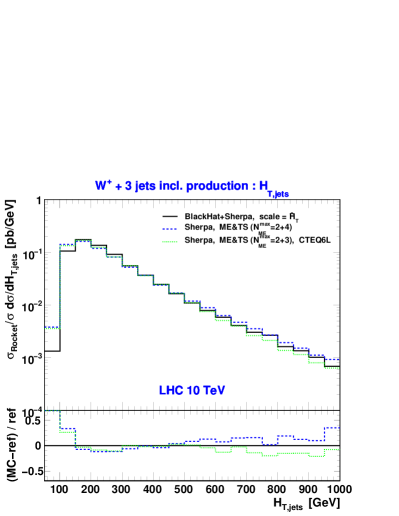
To get an idea of the impact of parton showering, we can analyze the matrix-element final states of the Sherpa ME&TS events (before they undergo showering) and plot distributions at the hard-process level, i.e. parton level, which we have labelled by “ME-level” in the plots. In the top left panel of Figure 18, we added the ME-level prediction (dotted turquoise line) to the first-jet $p_{T}$ spectra. It is in remarkable agreement with the NLO prediction of BlackHat+Sherpa over the entire range of the spectrum. As expected, the soft and collinear emissions added to the hard processes slightly soften the distribution such that the lower $p_{T}$ bins lie somewhat above the ME-level curve. There is almost no effect for bins of large $p_{T}$ as expected from IR-safe observables describing hard jets. Similar differences are found between Sherpa’s parton-shower- and ME-level curves for the $H_{T}$ observable presented in the left panel of Figure 19 where we use the definition $H_{T}=\sum_{\mathrm{jets}}p_{T,j}+p_{T,e}+\not{p}_{T}$. With or without shower effects included, all three predictions disagree for low $H_{T}$ values. Compared to the single-jet $p_{T}$s, the $H_{T}$ observable takes the leptons as well as multi-jet multi-particle correlations into account; it therefore contains more detailed information about the structure of the events. Apparently, these correlations and the generation of ($\geq$) 4-jet events are described differently by the three calculations. To gain more insight, one may investigate how the transverse momenta of the various jets are correlated. For large $H_{T}$, the BlackHat+Sherpa and ME&TS results agree quite well whereas the Rocket curve lies lower. A similar behaviour has been observed in [17] where distributions for both scale choices $\hat{H}_{T}$ and $E_{T,W}$ have been compared. The right panel of Figure 19 displays the $H_{T,\mathrm{jets}}$ distribution, which does not include the lepton and missing transverse momentum. As observed in the $p_{T}$ spectrum of the third jet, here as well, the prediction from the $N^{\mathrm{max}}_{\mathrm{ME}}=2+3$ ($N^{\mathrm{max}}_{\mathrm{ME}}=2+4$) merged sample lies below (above) the BlackHat+Sherpa curve.

Figure 20: The $p_{T}$ and rapidity spectra of the lepton (upper left and right), the neutrino’s $p_{T}$ spectrum and the reconstructed $W^{+}$ transverse-energy distribution (lower left and right) in inclusive $e^{+}\nu_{e}$ + 3 jet production at the LHC. NLO predictions as given by BlackHat+Sherpa (black line) and Rocket (red line) are compared to LO results from Sherpa using the ME&TS merging. All curves have been rescaled to the Rocket NLO cross section, cf. Table 5; the BlackHat+Sherpa prediction is used as the reference; for cuts and parameters, see Section 12.2

Figure 21: Pairwise geometric separations between the lepton and hardest jet (upper left panel) and the three hardest jets in $W^{+}$ + $\geq 3$ jet production at the LHC. BlackHat+Sherpa results at NLO (black lines) are compared to those of Sherpa’s ME&TS merging. The normalization is still given by Rocket’s NLO cross section of Table 5; the BlackHat+Sherpa prediction is used as the reference; for cuts and parameters, see Section 12.2

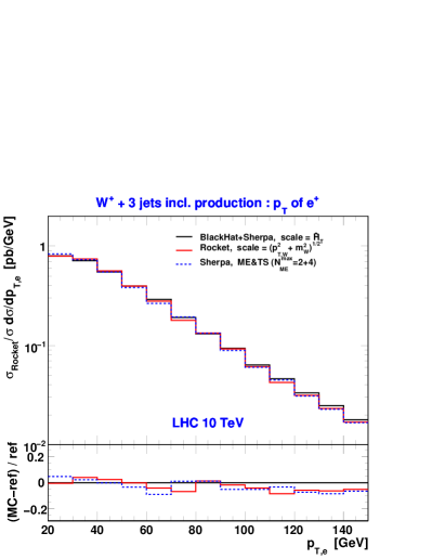
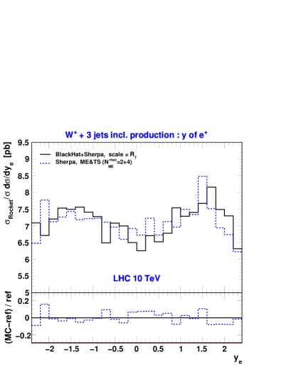
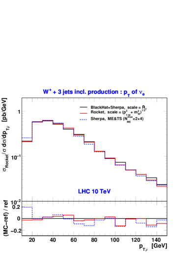
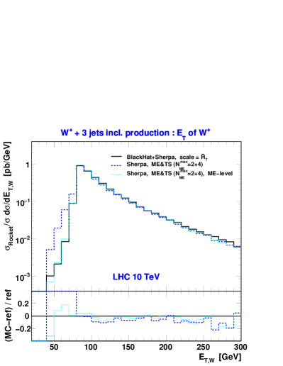
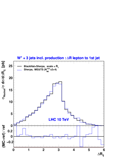
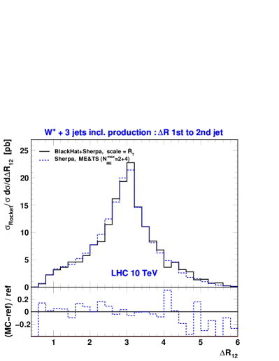
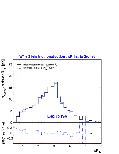
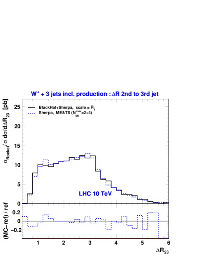
Figure 20 shows in the top row the positron transverse-momentum and rapidity distributions. The agreement between the different curves is rather satisfactory. This is also true for the missing transverse-momentum distribution shown in the lower left part of Figure 20. Here we do not anticipate larger differences between the two NLO scale choices and the ME&TS approach, as the plotted variables are directly related to the $W$ boson decay. In the lower right of Figure 20, the transverse energies of the reconstructed $W$ boson are compared. The clear difference at low $E_{T,W}$ between the BlackHat+Sherpa and Sherpa ME&TS curves is explained by the fact that the showers in the latter approach broaden the reconstructed mass peak of the $W$ boson. This is nicely confirmed by the ME-level result (dotted turquoise line) extracted as before from the ME&TS matrix-element final states.

We complete our main comparison by presenting $\Delta R$ shapes as given by the NLO computation of BlackHat+Sherpa and the ME&TS approach implemented in Sherpa. The results for the geometric separations between the lepton and leading jet as well as between pairs of the three hardest jets are shown in Figure 21. The predictions of both calculations are in remarkable agreement.

Figure 22: Impact of the variation of PDF and strong-coupling scales on Sherpa’s ME&TS merging for up to 4 jets shown by means of the third-jet $p_{T}$ (left) and $H_{T,\mathrm{jets}}$ distributions. The dotted dark and dashed green lines display the results for smaller and larger scales, respectively, also cf. Section 12.2 BlackHat+Sherpa is used as the reference, with the absolute normalization of all curves again given by Rocket’s NLO cross section even that no Rocket curve is shown.

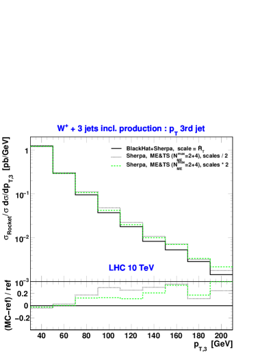
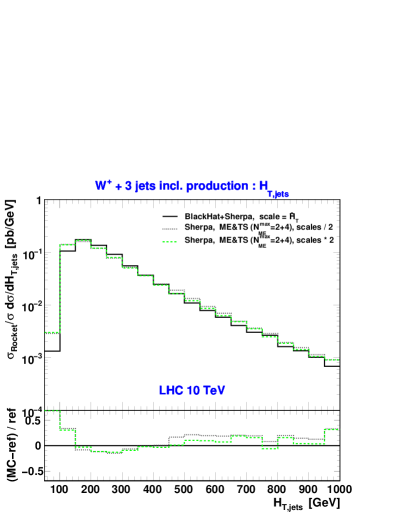
As we have seen in Figure 18, larger deviations between the NLO and ME&TS predictions appear in the third-jet transverse-momentum and $H_{T,\mathrm{jets}}$ distributions. For these observables, we present in Figure 22 scale variations of the ME&TS default scheme as described in the Sherpa paragraph of Section 12.2 The Sherpa shapes turn out to be rather stable varying not more than 20%. The reference curves given by BlackHat+Sherpa remain outside the uncertainty band. For a more conclusive statement, one should however also investigate the robustness of the NLO shapes under standard scale variations.

Figure 23: Comparison between NLO predictions as given by BlackHat+Sherpa (black lines) and Rocket (red lines) and LO results generated by Comix for the transverse momenta of the three hardest jets, $H_{T,\mathrm{jets}}$, the scalar sum of all jet $p_{T}$s, and the geometric separation $\Delta R_{12}$ of the two leading jets. The dashed magenta and green lines display LO results using $E_{T,W}$ and $H_{T}$ as a scale, respectively. The jet $p_{T}$ spectra also have coupling-reweighted LO curves taken from Ref. [126]. The absolute normalization of all curves is again given by Rocket’s NLO cross section; the reference is BlackHat+Sherpa’s prediction.

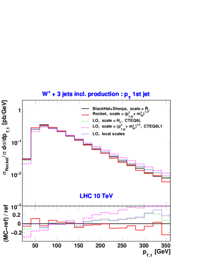
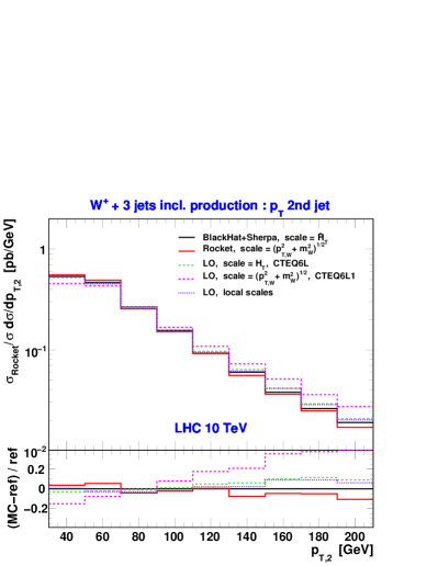
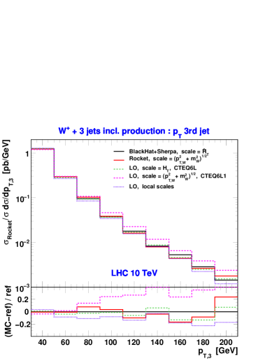
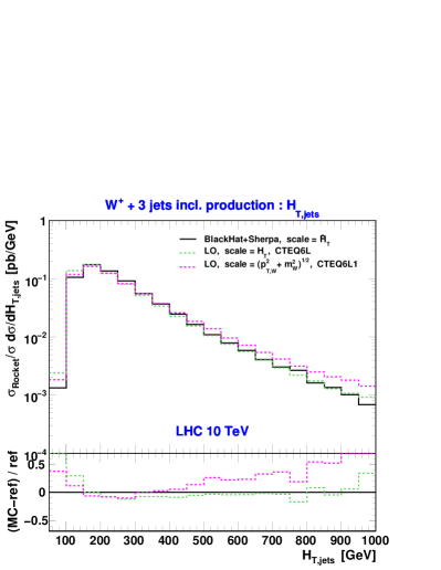
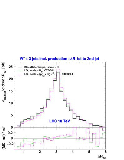
Finally, we turn to compare LO vs. NLO results for a subset of observables of our main comparison. We select those exhibiting the largest shape differences: the $p_{T}$ spectra of the hardest three jets, the $H_{T,\mathrm{jets}}$ distribution and the $\Delta R$ separation between the leading and next-to-leading jets. All of which are shown in Figure 23. The LO predictions using the scale choice $\mu=E_{T,W}$ lead in all cases to significant differences from the corresponding NLO predictions; jet pairs being narrow in $R$-space are predicted too low while the $p_{T}$ and $H_{T}$ spectra are too hard. Conversely, the LO predictions using $\mu=H_{T}$ as a scale are observed to produce relatively good agreement with NLO for the third-jet $p_{T}$ and $H_{T,\mathrm{jets}}$ shapes. The spectra for the leading and next-to-leading jets however overshoot the ones given at NLO although they are softer with respect to those arising from the $\mu=E_{T,W}$ scales. The $\Delta R_{12}$ curve has improved for low separations, still remains below the NLO result. In addition to the pure LO predictions, we have added to the $p_{T}$ spectra the coupling-reweighted LO results (LO, local scales) as presented in Ref. [126]. They have been obtained at LO by purely reweighting the initial strong couplings by those identified through $k_{T}$ backward clustering. The implementation used in [126] is in close spirit to the CKKW procedure [273, 274]. The results look very similar to the results at LO using $H_{T}$ as a scale, somewhat worse for the $p_{T}$ spectrum of the third jet. Compared to Figure 18 where we show the ME&TS results, one can conclude that the Sudakov rejections are the other important ingredient of the merging approach to improve the shapes of distributions and make them look similarly to those at NLO. The parton showers of ME&TS only correct in the soft/collinear phase-space regions.

12.4 Conclusions and outlook

We have presented a comparison of predictions for $W^{+}$ + $\geq 3$ jet production at the LHC with $\sqrt{s}=10$ TeV between the NLO programs BlackHat+Sherpa and Rocket and the ME&TS method of tree-level matrix-element plus parton-shower merging as implemented in Sherpa. This is the first time that results for this final state have been compared to each other. Despite the different inputs to these calculations, we have found an overall satisfactory agreement among the various predictions for the $p_{T}$ and $\eta$ shapes of jet and lepton distributions, and the jet–jet and jet-lepton $\Delta R$ correlations. The largest shape differences, of the order of 20% and 40%, are seen in the third-jet $p_{T}$ and $H_{T}$ distributions, respectively. These uncertainties might still be worrisome in the context of supersymmetry searches where $H_{T}$ is utilized as a major discriminating variable. As a matter of fact, the scale dependence on inclusive cross sections is considerably reduced at NLO; one still has to be careful to what extent the higher-order correction improves the predictions for more exclusive observables. The question for the “right” choice of scale(s) remains a tricky one to answer requiring more detailed studies.

As shown in Ref. [17], choosing the factorization and renormalization scales equal to the transverse energy of the $W$ boson can lead to unphysical (negative) results in the tails of some distributions. The effects at Tevatron energies are far less dramatic, as the range of the dynamical scales is much smaller there. It would be suggestive to extend our comparison to include higher transverse-energy bins in the plots to assess the potential danger of the $E_{T,W}$ scale choice.

The inclusive $W^{+}$ + $\geq 3$ jet cross sections given by the three computations vary between 34.2 pb for Rocket, 28.6 pb for BlackHat+Sherpa and 20.1 pb for Sherpa’s ME&TS implementation (with merging up to 4 jets). The neglect of subleading colour contributions in the Rocket calculation has been estimated to be less than 3%. Therefore, at NLO the main reason for the deviations certainly lies in the unequal scale choices, $E_{T,W}$ as used in Rocket and $\hat{H}_{T}$ as used in BlackHat+Sherpa, generating rather different average values for the $\mu_{\mathrm{F}}$ and $\mu_{\mathrm{R}}$ scales. The cross section given by the ME&TS merging in Sherpa is of leading-order nature, however, compared to the pure LO behaviour, it is more stable under the variation of scales and inclusion of tree-level matrix elements of higher order.

The LO kinematic shape distributions resulting from $H_{T}$ scales, rather than $E_{T,W}$ scales, resemble more closely those at NLO. In particular, we have observed relatively uniform differential $K$-factors for the third-jet $p_{T}$ and the $H_{T}$ variable. Hence, $H_{T}$ seems to serve as a scale that more correctly describes the overall hardness of the hard-scattering process. In summary: there is satisfactory agreement among the NLO predictions, even with the use of different scales, while there can be significant disagreement between LO and NLO predictions unless care is taken with the choice of the scales. Also, as a whole, the performance of the LO predictions is worse than that of Sherpa’s ME&TS merging. With sufficient tree-level matrix-element information, the ME&TS merging predictions given by Sherpa agree (in shape) with the NLO ones, indicating that the use of the correct local scale at each vertex mimics, to some extent, the full NLO behaviour. That similar results are obtained with the two very different scales is very interesting, and deserves further investigation than possible in this short write-up. It would be also very interesting to investigate the agreement between the NLO and ME&TS computations in a more detailed study that could include scale variations, different PDF choices and jet algorithms as well as a larger set of multi-particle correlations.

Acknowledgements

The authors would like to thank Jennifer Archibald, Carola F. Berger, Zvi Bern, John M. Campbell, Lance J. Dixon, R. Keith Ellis, Fernando Febres Cordero, Darren Forde, Walter T. Giele, Tanju Gleisberg, Harald Ita, David A. Kosower, Frank Krauss, Zoltan Kunszt, Joseph D. Lykken, Kirill Melnikov, Gavin P. Salam, Marek Schönherr, Steffen Schumann and Frank Siegert.

13 COMPARISON OF T-CHANNEL $2\rightarrow 3$ PRODUCTION AT NLO WITH COMPHEP SAMPLES

Single top quark production was recently observed for the first time by the D0 [275] and CDF [276] collaborations at the Tevatron proton-antiproton collider at Fermilab. Two Feynman diagrams for single top quark production at a hadron collider are shown in Fig. 24: (a) the leading order ($2\rightarrow 2$) exchange of a $W$ boson between a light quark line and a heavy quark line, and (b) the ($2\rightarrow 3$) process where this $b$ quark explicitly comes from gluon splitting. Diagram (a) is also referred to as single top production in the 5-flavor scheme because it utilizes the $b$ quark parton distribution function (PDF) in the proton. Diagram (b) is also referred to as $W$-gluon-fusion or single top production in the 4-flavor scheme because the PDF of the gluon is required rather than the PDF of the $b$ quark. While the $2\rightarrow 3$ process (b) is one of the NLO corrections to the LO process (a), it is an important contribution and the dominant contribution when explicitly requiring three reconstructed jets.

Figure 24: Feynman diagram for $t$-channel single top quark production, in the $2\rightarrow 2$ scheme (a) and the $2\rightarrow 3$ scheme (b).

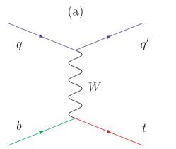
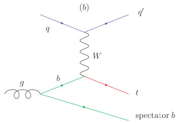
A calculation of t-channel single top quark production at NLO in the $2\rightarrow 3$ scheme is now available, based on the MCFM NLO calculation [277]. This is the first calculation providing $O(\alpha_{s})$ corrections to the spectator $b$ quark from gluon splitting in the t-channel process. Here we compare the distributions of this spectator $b$ quark with t-channel single top samples generated with the CompHEP SingleTop generator [278, 279]. These samples are used by the D0 experiment, for example in the observation of single top quark production [275].

In the CompHEP generation, both $2\rightarrow 2$ processes (eg $qb\rightarrow q^{\prime}t$, Fig. 24(a)) and $2\rightarrow 3$ processes (eg $qg\rightarrow q^{\prime}t\overline{b}$, Fig. 24(b)) are included. The $2\rightarrow 3$ process is relevant when the spectator $b$ quark is central and at high $p_{T}$ and can be observed in the detector. The $2\rightarrow 2$ processes start from a $b$-quark parton distribution function (PDF) and are relevant when the spectator $b$ quark is soft and cannot be observed in the detector. These two contributions need to be combined to provide one inclusive simulation sample. In the CompHEP matching approach [278, 279], both samples are processed by Pythia [280], and the $p_{T}$ distributions of the spectator $b$ quark produced by Pythia are matched at a given spectator $b$ quark $p_{T}$ threshold. Below this threshold, the $2\rightarrow 2$ sample is used, whereas above the threshold, the $2\rightarrow 3$ sample is used. The threshold is chosen to produce a smooth $p_{T}$ distribution, typically between 10GeV and 20GeV. In this particular example it is at 17 GeV. The CompHEP sample was generated at a top quark mass of 172.5GeV, using the CTEQ 6.1 PDF set [171].

The MCFM samples were generated at a top quark mass of 170GeV and the CTEQ6M PDF set. There is a small difference in top quark mass between the two samples, but this has a negligible impact on the spectator $b$ quark kinematics.

Figure 25: Comparison of the $p_{T}$ of the spectator quark in $t$-channel single top quark production between the MCFM $2\rightarrow 3$ NLO calculation and CompHEP interfaced to Pythia, in linear scale (left) and in log scale (right). Each distribution is normalized to the NLO cross section.

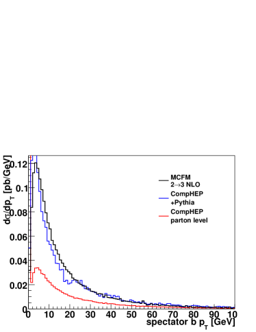
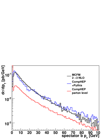
Figure 25 shows a comparison of the transverse momentum ($p_{T}$) of the spectator quark. No cuts have been applied. The CompHEP parton level spectator $b$ quark $p_{T}$ distribution has a large spike at zero from $2\rightarrow 2$ events that have no spectator $b$ quark at parton level. The CompHEP $2\rightarrow 3$ contribution at parton level is significantly below the MCFM calculation. However, once initial and final state gluon radiation is added by Pythia, the spectator $b$ quark distribution agrees well with the MCFM calculation. The main effect of Pythia is to shift the $2\rightarrow 3$ contribution to the right and to fill in the low $p_{T}$ region with the $2\rightarrow 2$ calculation.

Figure 26: Comparison of the pseudorapidity distribution of the spectator quark in $t$-channel single top quark production between the MCFM $2\rightarrow 3$ NLO calculation and CompHEP interfaced to Pythia.

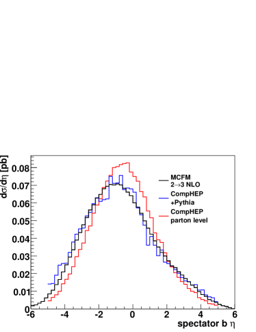
Figure 26 shows a comparison of the pseudorapidity of the spectator $b$ quark. As explained above, the CompHEP parton level distribution consists only of $2\rightarrow 3$ events, but even here the agreement with the NLO calculation is reasonable. The Pythia output again agrees well with the NLO calculation.

We have also calculated the acceptance for a spectator $b$ quark cut of $p_{T}>20$ GeV and a pseudorapidity cut of $|\eta|<2.8$, following the approach of Ref. [281]. We obtain an acceptance of 31.6% for the Pythia output samples, in good agreement with the MCFM NLO calculation [281].

In summary, we have presented a comparison of spectator $b$ quark in $t$-channel single top quark production between the CompHEP parton-level event generator interfaced to Pythia and the MCFM NLO calculation of the $t$-channel $2\rightarrow 3$ process. We find good agreement between the Pythia output and MCFM for the spectator $b$ quark kinematics.

14 TUNED COMPARISON OF NLO QCD CORRECTIONS TO $pp\to ZZ{+}\mathrm{jet}{+}X$ PRODUCTION AT HADRON COLLIDERS

14.1 Introduction

The complicated hadron collider environment of the LHC requires not only sufficiently precise predictions for the expected signals, but also reliable rates for complicated background reactions, especially for those that cannot be entirely measured from data. Among such background processes, several involve three, four, or even more particles in the final state, rendering the necessary next-to-leading-order (NLO) calculations in QCD technically challenging. At the previous Les Houches workshops this problem led to the creation of a list of calculations that are a priority for LHC analyses, the so called ”experimenters’ wishlist for NLO calculations” [2, 1, 3]. The process class of ’electroweak gauge-boson pair with a hadronic jet’ made it to the top of this list. Among other processes of that class, which have been addressed in earlier works [4, 5, 6, 282], the process $pp\to ZZ{+}\text{jet}{+}X$ is of interest, for example as a background process to $H$+jet with the Higgs boson decaying into a pair of $Z$ bosons.

First results on the calculation of NLO QCD corrections to $ZZ$+jet production have been presented in Ref. [7]. A second calculation is in progress [283] with some results already presented in Ref. [284]. In the following the key features of these two independent calculations are described and results of an ongoing tuned comparison are presented.

14.2 Descriptions of the various calculations

At leading order (LO), hadronic $ZZ$+jet production receives contributions from the partonic processes $q\bar{q}\to ZZg$, $qg\to ZZq$, and $\bar{q}g\to ZZ\bar{q}$, where $q$ stands for up- or down-type quarks. All three channels are related by crossing symmetry.

The virtual corrections modify the partonic processes that are already present at LO. At NLO these corrections are induced by self-energy, vertex, box (4-point), and pentagon (5-point) corrections, the latter being the most complicated loop diagrams. Apart from an efficient handling of the huge amount of algebra, the most subtle point certainly is the numerically stable evaluation of the numerous tensor loop integrals, in particular in the vicinity of exceptional phase-space points. The two calculations described below employ completely different loop methods. Some of them are already briefly reviewed in Ref. [2], where more details on problems in multi-leg loop calculations and brief descriptions of proposed solutions can be found.

The real corrections are induced by the large variety of processes that result from crossing any pair of QCD partons in $0\to ZZq\bar{q}gg$ and $0\to ZZq\bar{q}q^{\prime}\bar{q}^{\prime}$ into the initial state. Here the main complication in the evaluation is connected to an efficient phase-space integration with a proper separation of soft and collinear singularities. For the separation of singularities the two calculations both employ the subtraction method[285] using the dipole subtraction formalism of Catani and Seymour[168].

The calculation of DKU [284, 283]

This calculation is actually based on two completely independent evaluations of the virtual and real corrections, referred to as DKU1 and DKU2 below. The $Z$ bosons are taken to be on shell since the discussed results do not depend on the details of the $Z$ decays. Both evaluations of loop diagrams are performed analogously to the calculations for the related process of $WW$+jet production, which are discussed in Refs. [4, 5].

The first calculation essentially follows the same strategy already applied to the processes of $t\bar{t}H$ [187] and $t\bar{t}{+}\mathrm{jet}$ [177] production: The amplitudes are generated by FeynArts 1.0 [286] and further processed with in-house Mathematica routines, which automatically create an output in Fortran. The IR (soft and collinear) singularities are treated in dimensional regularization and analytically separated from the finite remainder as described in Refs. [187, 287]. The pentagon tensor integrals are directly reduced to box integrals following Refs. [101, 100]. Box and lower-point integrals are reduced à la Passarino–Veltman [133] to scalar integrals, which are either calculated analytically or using the results of Refs. [288, 289, 95].

The second loop calculation is based on FeynArts 3.4 [149] to generate the diagrams and FormCalc 6.0 [148] which automatically produces Fortran code. The reduction of tensor to scalar integrals is done with the help of the LoopTools library [148], which also employs the method of Ref. [101] for the 5-point tensor integrals, Passarino–Veltman [133] reduction for the lower-point tensors, and the FF package [150, 290] for the evaluation of regular scalar integrals. The dimensionally regularized soft or collinear singular 3- and 4-point integrals had to be added to this library.

The first calculation of the real corrections employs analytical results for helicity amplitudes obtained in a spinor formalism. The phase-space integration is performed by the multi-channel Monte Carlo integrator [291] with weight optimization [292] that has been written in C++ and tested in the calculation of $WW$+jet. More details on this calculation and some numerical results can be found in Ref. [284].

The second evaluation of the real corrections is based on scattering amplitudes calculated with Madgraph [164] generated code. The code has been modified to allow for the extraction of the required colour and spin structure. The latter enter the evaluation of the dipoles in the Catani–Seymour subtraction method. The evaluation of the individual dipoles was performed using a C++ library developed during the calculation of the NLO corrections for $t\bar{t}{+}\mathrm{jet}$ [177]. For the phase-space integration a simple mapping has been used where the phase space is generated from a sequential splitting.

The calculation of BGKKS [7]

This calculation is based on two independent sets of amplitude expressions: one generated manually starting from the Feynman graph representation, the other using QGRAF [151]. Both representations employ the spinor helicity formalism of Ref. [293]. Polarisation vectors have been represented via spinor traces, i.e. kinematic invariants up to global phases. By obtaining an analytical representation for the full amplitude, we aim at promoting simplification via analytical cancellations. Especially we employ that, apart from the rank one case, all pentagon tensor integrals are reducible, i.e. can directly be written as simple combinations of box tensor integrals. For the remaining tensor integrals we employ the GOLEM-approach [147, 146, 137]. In this approach, the use of 6-dimensional IR finite box functions allows to isolate IR divergences in 3-point functions. We use FORM [138] and Maple to obtain tractable analytical expressions for the coefficients to the employed set of basis functions for each independent helicity amplitude, and to further simplify them. The basis functions are evaluated using the GOLEM95 implementation [102]. We note that for the reduction of box topologies one obtains the same result as with the Passarino-Veltman tensor reduction [288, 133]. If one fully reduces all tensor integrals to a scalar integral representation, the difference between the two approaches results from the treatment of the pentagon integrals and the use of finite 6-dimensional box functions.

To treat $\gamma_{5}$ we employ the ’t Hooft-Veltman scheme [294, 295], where the $\gamma^{\mu}$ are split into a 4-dimensional part that anti-commutes with $\gamma_{5}$ and a commuting remainder. As is well known, to take into account differences between the QCD corrections to axial vector and vector currents, a finite renormalization has to be performed. To enforce the correct chiral structure of the amplitudes, a finite counterterm for the axial part is included in the used gauge boson vertex (see e.g. Refs. [296, 297, 298]):

$$V^{\mu}_{Vq\bar{q}}\sim g_{v}\,\gamma^{\mu}+Z_{5}\,g_{a}\,\gamma^{\mu}\gamma_{5}\quad\text{with}\quad Z_{5}=1-C_{F}\,\frac{\alpha_{s}}{\pi}\,.$$

We calculate with $N_{\mathrm{f}}=5$ and neglect quark mass effects. Our virtual amplitudes have been verified by comparing two independent internal implementations, both generated using the GOLEM reduction. We have verified that the relative contribution of graphs with quark loops to integrated results is typically well below 1%. We therefore neglect this contribution. To calculate numerical results for the virtual contributions we employed the OmniComp-Dvegas package, which facilitates parallelised adaptive Monte Carlo integration and was developed in the context of Ref. [299]. We use the SHERPA implementation [267, 300, 132] to calculate numerical results for the finite real corrections contribution. All amplitude and dipole contributions have been verified through comparison with results calculated with MadDipole/MadGraph [166, 164] and HELAC [196, 193].

14.3 Tuned comparison of results

The following results essentially employ the setup of Ref. [7]. The CTEQ6 [171, 197] set of parton distribution functions (PDFs) is used throughout, i.e. CTEQ6L1 PDFs with a 1-loop running $\alpha_{\mathrm{s}}$ are taken in LO and CTEQ6M PDFs with a 2-loop running $\alpha_{\mathrm{s}}$ in NLO. In the strong coupling constant the number of active flavours is $N_{\mathrm{f}}=5$, and we use the default LHAPDF values leading to $\alpha_{\mathrm{s}}^{\mathrm{LO}}(91.188\text{ GeV})=0.129783$ and $\alpha_{\mathrm{s}}^{\mathrm{NLO}}(91.70\text{ GeV})=0.1179$. The top-quark loop in the gluon self-energy is subtracted at zero momentum. The running of $\alpha_{\mathrm{s}}$ is, thus, generated solely by the contributions of the light quark and gluon loops. In all results shown in the following, the renormalization and factorization scales are set to $M_{Z}$. The top-quark mass is $m_{t}=174.3$ GeV, the masses of all other quarks are neglected. The weak boson masses are $M_{Z}=91.188$ GeV and $M_{H}=150$ GeV. The weak mixing angle is set to its on-shell value, i.e. fixed by $s_{w}^{2}=0.222247$, and the electromagnetic coupling constant is set to $\alpha=0.00755391226$.

We apply the $k_{\perp}$ jet algorithm of Ref. [199] with covariant $E$-recombination scheme and $R=0.7$ for the definition of the tagged hard jet and restrict the transverse momentum of the hardest jet by $p_{\mathrm{T,jet}}>50$ GeV.

14.3.1 Results for a single phase-space point

For the comparison the following set of four-momenta $(E,p_{x},p_{y},p_{z})$ [GeV] is chosen,

$$p_{1}^{\mu} =(250,0,0,250),\qquad p_{2}^{\mu}=(250,0,0,-250),$$ (49)

$$p_{3}^{\mu} =(125.9335600344245,-81.91900733932759,-15.22986911133704,-24.52218428963296),$$

$$p_{4}^{\mu} =(201.2131630027446,37.57875773939030,-105.1640094872687,140.3561672919824),$$

$$p_{5}^{\mu} =(172.8532769628309,44.34024959993729,120.3938785986057,-115.8339830023494),$$

where incoming and outgoing particles are labelled as follows: $1,2\to 3,4,5$.

Table 6 shows some results for the spin- and colour-summed squared LO matrix elements, where no factor $1/2$ is included for the two identical $Z$ bosons in the final state. The results of the two groups  agree within about 13 digits.

	$|{\cal M}_{\mathrm{LO}}|^{2}/e^{4}/g_{\mathrm{s}}^{2}[\mathrm{GeV}^{-2}]$
$u\bar{u}\to ZZg$
BGKKS	$9.081603376311467\cdot 10^{-4}$
DKU1	$9.081603376315696\cdot 10^{-4}$
DKU2	$9.081603376315669\cdot 10^{-4}$
$d\bar{d}\to ZZg$
BGKKS	$1.892589730735170\cdot 10^{-3}$
DKU1	$1.892589730736050\cdot 10^{-3}$
DKU2	$1.892589730736046\cdot 10^{-3}$
$ug\to ZZg$
BGKKS	$1.687614989680196\cdot 10^{-4}$
DKU1	$1.687614989680182\cdot 10^{-4}$
DKU2	$1.687614989680173\cdot 10^{-4}$
$dg\to ZZg$
BGKKS	$3.516959138773490\cdot 10^{-4}$
DKU1	$3.516959138773458\cdot 10^{-4}$
DKU2	$3.516959138773441\cdot 10^{-4}$
$g\bar{u}\to ZZg$
BGKKS	$1.319241114194492\cdot 10^{-5}$
DKU1	$1.319241114194495\cdot 10^{-5}$
DKU2	$1.319241114194489\cdot 10^{-5}$
$g\bar{d}\to ZZg$
BGKKS	$2.749274639763224\cdot 10^{-5}$
DKU1	$2.749274639763229\cdot 10^{-5}$
DKU2	$2.749274639763217\cdot 10^{-5}$

Table 6: Results for squared LO matrix elements at the phase-space point (49).

	$c^{\mathrm{bos}}_{0}[\mathrm{GeV}^{-2}]$	$c^{\mathrm{ferm1+2}}_{0}[\mathrm{GeV}^{-2}]$	$c^{\mathrm{ferm3}}_{0}[\mathrm{GeV}^{-2}]$
$u\bar{u}\to ZZg$
BGKKS	$2.571718370986939\cdot 10^{-4}$	$2.771274006707126\cdot 10^{-6}$
DKU1	$2.571718370988091\cdot 10^{-4}$	$2.771273991103833\cdot 10^{-6}$	$3.301195986341516\cdot 10^{-6}$
DKU2	$2.571718370988072\cdot 10^{-4}$	$2.771273991102529\cdot 10^{-6}$	$3.301195986341134\cdot 10^{-6}$
$d\bar{d}\to ZZg$
BGKKS	$5.335637852921577\cdot 10^{-3}$	$3.553804947755081\cdot 10^{-6}$
DKU1	$5.335637852923933\cdot 10^{-3}$	$3.553804924505993\cdot 10^{-6}$	$-7.625169350877288\cdot 10^{-6}$
DKU2	$5.335637852923915\cdot 10^{-3}$	$3.553804924504350\cdot 10^{-6}$	$-7.625169350877653\cdot 10^{-6}$
$ug\to ZZg$
BGKKS	$3.455303690923093\cdot 10^{-4}$	$-1.575277709579237\cdot 10^{-6}$
DKU1	$3.455303690940059\cdot 10^{-4}$	$-1.575277712403393\cdot 10^{-6}$	$-1.899597362881991\cdot 10^{-6}$
DKU2	$3.455303690940080\cdot 10^{-4}$	$-1.575277712403507\cdot 10^{-6}$	$-1.899597362882020\cdot 10^{-6}$
$dg\to ZZg$
BGKKS	$7.182218731401221\cdot 10^{-4}$	$-2.134836868278616\cdot 10^{-6}$
DKU1	$7.182218731436469\cdot 10^{-4}$	$-2.134836871947412\cdot 10^{-6}$	$3.857433911012773\cdot 10^{-6}$
DKU2	$7.182218731436517\cdot 10^{-4}$	$-2.134836871947570\cdot 10^{-6}$	$3.857433911012694\cdot 10^{-6}$
$g\bar{u}\to ZZg$
BGKKS	$7.284079447744509\cdot 10^{-5}$	$-3.877856878313408\cdot 10^{-6}$
DKU1	$7.284079439746620\cdot 10^{-5}$	$-3.877856878314387\cdot 10^{-6}$	$-5.478348291183621\cdot 10^{-7}$
DKU2	$7.284079439746720\cdot 10^{-5}$	$-3.877856878314465\cdot 10^{-6}$	$-5.478348291184200\cdot 10^{-7}$
$g\bar{d}\to ZZg$
BGKKS	$1.505448756089957\cdot 10^{-5}$	$-4.839140375435081\cdot 10^{-6}$
DKU1	$1.505448754415003\cdot 10^{-5}$	$-4.839140375436319\cdot 10^{-6}$	$3.379222628266236\cdot 10^{-7}$
DKU2	$1.505448754415026\cdot 10^{-5}$	$-4.839140375436448\cdot 10^{-6}$	$3.379222628265571\cdot 10^{-7}$

Table 7: Virtual corrections of the bosonic contributions, the fermionic contributions of the two light generations ($m_{q}=0$), and the fermionic contributions of the $3^{\rm{rd}}$ generation ($m_{\rm{b}}=0$, $m_{\rm{t}}=174.3$ GeV) at the phase-space point (49).

In order to be independent of the subtraction scheme to cancel IR divergences, we found it useful to compare virtual results prior to any subtraction. The ${\cal O}(\alpha_{s})$ contribution to the virtual, renormalized squared amplitude is given by the interference between tree-level and one-loop virtual amplitude, which we denote schematically as

$$2\mathrm{Re}\{{\cal M}_{V}^{*}\cdot{\cal M}_{\mathrm{LO}}\}=e^{4}g_{s}^{2}f(\mu_{\mathrm{ren}})\left(c_{-2}\frac{1}{\epsilon^{2}}+c_{-1}\frac{1}{\epsilon}+c_{0}\right)\,,$$ (50)

with $f(\mu_{\mathrm{ren}})=\Gamma(1+\epsilon)(4\pi\mu_{\mathrm{ren}}^{2}/M_{Z}^{2})^{\epsilon}$ and the number of space–time dimensions $D=4-2\epsilon$. In the following we split the coefficients of the double and single pole and for the constant part, $c_{-2},c_{-1}$, and $c_{0}$, into bosonic contributions (“bos”) without closed fermion loops and the remaining fermionic parts. The fermionic corrections are further split into contributions from the first two generations (“ferm1+2”) and from the third generation (“ferm3”).

The results on $c_{0}$ obtained by the different groups typically agree within $8{-}12$ digits; the agreement between DKU1 and DKU2 results turns out to be within $12{-}14$ digits. The values of $c_{0}$ for the different channels are collected in Table 7 according to the splitting stated above. The coefficients of the poles have not been compared numerically since the cancellation of divergences can be checked analytically.

14.3.2 Results for integrated cross sections

Table 8 illustrates the agreement of the LO and NLO cross sections for the LHC ($pp$, $\sqrt{s}=14$ TeV) and Tevatron ($p\bar{p}$, $\sqrt{s}=1.96$ TeV) calculated by both groups with the setup defined above. For the NLO observable labelled by ’excl’, a veto on a $2^{\rm{nd}}$ hard jet ($p_{\mathrm{T,2^{nd}\,jet}}<50\,\rm{GeV}$) has been applied in the real-correction contribution.

Table 9 provides individual contributions to the NLO cross section in Table 8, as well as the contribution of the fermionic loops to the integrated NLO cross section—again subdivided into contributions of the two light generations and the third one—, which have not been taken into account in the cross sections of Table 8. However, their size turns out to be well below the percent level, so that they may be neglected on the experimentally required level of accuracy.

We note that we also compared cross sections for different scale choices and distributions and found agreement.

$pp\to ZZ{+}\mathrm{jet}{+}X$ @ LHC	$\sigma_{\mathrm{LO}}$[fb]	$\sigma_{\mathrm{NLO}}$[fb]	$\sigma_{\mathrm{NLO,excl}}$[fb]
BGKKS	$2697.82\,[42]$	$3644.5\,[3.0]$	$2627.5\,[3.0]$
DKU	$2697.81\,[18]$	$3644.6\,[1.0]$	$2626.3\,[1.1]$
$p\bar{p}\to ZZ{+}\mathrm{jet}{+}X$ @ Tevatron	$\sigma_{\mathrm{LO}}$[fb]	$\sigma_{\mathrm{NLO}}$[fb]	$\sigma_{\mathrm{NLO,excl}}$[fb]
BGKKS	$74.5589\,[90]$	$83.665\,[62]$	$78.824\,[62]$
DKU	$74.5664\,[76]$	$83.751\,[47]$	$78.915\,[47]$

Table 8: Results for contributions to the integrated $ZZ$+jet cross sections at the LHC and Tevatron in LO and NLO. Only bosonic loop corrections are included here in the virtual part, i.e. all fermion loops are neglected.

	$pp\to ZZ{+}\mathrm{jet}{+}X$ @ LHC		$p\bar{p}\to ZZ{+}\mathrm{jet}{+}X$ @ Tevatron
	BGKKS	DKU	BGKKS	DKU
$\sigma_{\mathrm{born}}$[fb]	$2580.60\,\phantom{.}[39]$	$2579.91\,[55]\phantom{0}$	$70.0581\,[83]$	$70.056\,[23]\phantom{00}$
$\sigma_{\mathrm{coll}}$[fb]	$918.62\,\phantom{.}[54]$	$917.59\,[39]\phantom{0}$	$16.578\,[24]\phantom{0}$	$16.592\,[17]\phantom{00}$
$\sigma_{\mathrm{real}}$[fb]	$-82.9\,[2.4]\phantom{0}$	$-82.79\,[72]\phantom{0}$	$-11.143\,[26]\phantom{0}$	$-11.092\,[36]\phantom{00}$
$\sigma_{\mathrm{real,excl}}$[fb]	$-1099.9\,[2.4]\phantom{0}$	$-1101.09\,[76]\phantom{0}$	$-15.983\,[26]\phantom{0}$	$-15.928\,[36]\phantom{00}$
$\sigma_{\mathrm{virt,\,bose+I}}$[fb]	$228.1\,[1.7]\phantom{0}$	$229.92\,[34]\phantom{0}$	$8.171\,[50]\phantom{0}$	$8.1950\,[88]\phantom{0}$
$\sigma_{\mathrm{virt,\,ferm\,1+2}}$[fb]		$-17.864\,[28]$		$-0.07527\,[11]$
$\sigma_{\mathrm{virt,\,ferm\,3}}$[fb]		$6.750\,[16]$		$0.18600\,[14]$

Table 9: Results for the born, sum of the $K$ and $P$ insertion operators, dipole subtracted real emissions, IR-finite sum of bosonic loops and the $I$ insertion operator and fermion loops contributions to the integrated $ZZ$+jet cross sections in NLO at the LHC and Tevatron.

14.4 Conclusions

We have reported on a tuned comparison of calculations of the NLO QCD corrections to $ZZ$+jet production at the LHC and Tevatron. For a fixed phase-space point, the virtual corrections obtained by both groups using different calculational techniques agree at the level of $10^{-8}$ or better. The comparison of full NLO cross sections, which involve the non-trivial integration of virtual and real corrections over the phase space, shows agreement at the permille level.

Acknowledgements

This work is supported in part by the EU’s Marie-Curie Research Training Network HEPTOOLS under contract MRTN-CT-2006-035505 and by Germany’s DFG (SFB/TR9 and contract BI 1050/2) and BMBF (contract 05HT1WWA2), the UK’s HEFCE, STFC and SUPA and the US DOE (contract DE-AC02-76SF00515).

15 W PAIR PRODUCTION: NNLO VIRTUAL CORRECTIONS WITH FULL MASS DEPENDENCE

15.1 Introduction

One of the primary goals for the LHC is undoubtedly the discovery of the Higgs boson which is responsible for the fermions and gauge bosons mass and also part of the mechanism of dynamical breaking of the Electroweak (EW) symmetry. Another important aim for the LHC is the precise measurement of the hadronic production of gauge boson pairs, $WW$, $WZ$, $ZZ$, $W\gamma$, $Z\gamma$, this in connection to the investigation of the non-Abelian gauge structure of the SM. W pair production,

$$q{\bar{q}}\rightarrow W^{+}\,W^{-}\,,$$ (51)

plays an essential role as it serves as a signal process in the search for New Physics and also is the dominant irreducible background to the promising Higgs discovery channel

$$pp\rightarrow H\rightarrow W^{*}W^{*}\rightarrow l{\bar{\nu}}{\bar{l}}^{\prime}\nu^{\prime}\,$$ (52)

in the mass range $M_{\mathrm{Higgs}}$ between 140 and 180 GeV [301].

The process is currently known at next-to-leading order (NLO) accuracy [302, 303, 304, 305, 306, 307, 308]. The NLO corrections were proven to be large enhancing the tree-level by almost 70% which falls to a (still) large 30% after imposing a jet veto. Therefore, if a theoretical estimate for the W pair production is to be compared against experimental measurements at the LHC, one is bound to go one order higher in the perturbative expansion, namely, to the next-to-next-to-leading order (NNLO). This would allow, in principle, an accuracy of around 10%.

High accuracy for the W pair production is also needed when the process is studied as background to Higgs production in order to match accuracies between signal and background. The signal process for the Higgs discovery via gluon fusion, $gg\rightarrow H$, as well as the process $H\rightarrow WW\rightarrow l{\bar{\nu}}{\bar{l}}^{\prime}\nu^{\prime}$ are known at NNLO [309, 310, 311, 312, 313, 314, 315, 316, 317, 318], whereas the EW corrections are known beyond NLO [319]. Another process that needs to be included in the background is the W pair production in the loop induced gluon fusion channel,

$$gg\rightarrow W^{+}W^{-}\,.$$ (53)

The latter contributes at $\mathcal{O}(\alpha_{s}^{2})$ relative to the quark-anti-quark-annihilation channel but is nevertheless enhanced due to the large gluon flux at the LHC [320, 321].

The first main difficulty in studying the NNLO QCD corrections for W pair production is the calculation of the two-loop virtual amplitude since it is a $2\rightarrow 2$ process with massive external particles. We have already computed the virtual corrections at the high energy limit [322, 323, 324]. However, this is not enough as it cannot cover the kinematical region close to threshold. Therefore, in order to cover all kinematical regions we proceed as follows. We perform a deep expansion in the W mass around the high energy limit which in combination with the method of numerical integration of differential equations [325, 326, 327] allows us the numerical computation of the two-loop amplitude with full mass dependence over the whole phase space.

15.2 The high energy limit

The methodology for obtaining the massive amplitude in the high energy limit, namely the limit where all the invariants are much larger than the W mass, is similar to the one followed in Refs. [328, 329]. The amplitude is reduced to an expression that only contains a small number of integrals (master integrals) with the help of the Laporta algorithm [330]. In the calculation for the two-loop amplitude there are 71 master integrals. Next step is the construction, in a fully automatised way, of the Mellin-Barnes (MB) representations [331, 332] of all the master integrals by using the MBrepresentation package [333]. The representations are then analytically continued in the number of space-time dimensions by means of the MB package [334], thus revealing the full singularity structure. An asymptotic expansion in the mass parameter (W mass) is performed by closing contours and the integrals are finally resummed, either with the help of XSummer [255] or the PSLQ algorithm [335]. The result is expressed in terms of harmonic polylogarithms.

15.3 Power corrections and numerical evaluation

The high energy limit by itself is not enough, as was mentioned before. The next step, following the methods applied in Ref. [336], is to compute power corrections in the W mass. Power corrections are good enough to cover most of the phase space, apart from the region near threshold as well as the regions corresponding to small angle scattering.

We recapitulate here some of the notation of Ref. [324] for completeness. The charged vector-boson production in the leading partonic scattering process corresponds to

$$q(p_{1})+{\overline{q}}(p_{2})\>\>\rightarrow\>\>W^{-}(p_{3},m)+W^{+}(p_{4},m)\,,$$ (54)

where $p_{i}$ denote the quark and W momenta and $m$ is the mass of the W boson.

We have chosen to express the amplitude in terms of the kinematic variables $x$ and $m_{s}$ which are defined to be

$$x=-\frac{t}{s},\;\;m_{s}=\frac{m^{2}}{s},$$ (55)

where

$$s=(p_{1}+p_{2})^{2}\;\;{\rm and}\;\;t=(p_{1}-p_{3})^{2}-m^{2}\,.$$ (56)

The variation then of $x$ within the range $[1/2(1-\beta),1/2(1+\beta)]$, where $\beta=\sqrt{1-4m^{2}/s}$ is the velocity, corresponds to angular variation between the forward and backward scattering.

It should be evident that any master integral $M_{i}$ can be written then as

$$M_{i}=M_{i}\left(m_{s},x,\epsilon\right)=\sum_{j=k}^{l}\epsilon^{j}{I_{i}}_{j}(m_{s},x),$$ (57)

where the lowest power of $\epsilon$ in the sum can be $-4$.

The crucial point now is that the derivative of any Feynman integral with respect to any kinematical variable is again a Feynman integral with possibly higher powers of denominators or numerators which can also be reduced to masters from the initial set of master integrals. This means that one can construct a partially triangular system of differential equations in the mass, which can subsequently be solved in the form of a power series expansion, with the expansion parameter in our case being $m_{s}$ following the conventions above.

Let us differentiate with respect to $m_{s}$ and $x$, we will then have respectively

$$m_{s}\frac{d}{dm_{s}}M_{i}(m_{s},x,\epsilon)=\sum_{j}C_{ij}(m_{s},x,\epsilon)~{}M_{j}(m_{s},x,\epsilon)$$ (58)

and

$$x\frac{d}{dx}M_{i}(m_{s},x,\epsilon)=\sum_{j}C_{ij}^{\prime}(m_{s},x,\epsilon)~{}M_{j}(m_{s},x,\epsilon)\,.$$ (59)

We use Eq. (58) to obtain the mass corrections for the masters calculating the power series expansion up to order $m_{s}^{11}$ (see also Ref. [336] for more details). This deep expansion in $m_{s}$ should be sufficient for most of the phase space but still not enough to cover the whole allowed kinematical region. The way to proceed from this point is to numerically integrate the system of differential equations.

In particular, we choose to work with the masters in the form of Eq. (57), where the $\epsilon$ dependence is explicit. We can then work with the coefficients of the $\epsilon$ terms and accordingly have

$$m_{s}\frac{d}{dm_{s}}I_{i}(m_{s},x)=\sum_{j}J^{M}_{ij}(m_{s},x)~{}I_{j}(m_{s},x)$$ (60)

and

$$x\frac{d}{dx}I_{i}(m_{s},x)=\sum_{j}J^{X}_{ij}(m_{s},x)~{}I_{j}(m_{s},x),$$ (61)

where the Jacobian matrices $J^{M}$ and $J^{X}$ have rational function elements.

By using this last system of differential equations, one can obtain a full numerical solution to the problem. What we are essentially dealing now with is an initial value problem and the main requirement is to have the initial conditions to proper accuracy. The initial conditions, namely the values of the masters at a proper kinematical point which we call initial point, are provided by the power series expansion. The initial point has to be chosen somewhere in the high energy limit region, where $m_{s}$ is small and therefore, the values obtained by the power series are very accurate. Starting from there, one can evolve to any other point of the phase space by numerically integrating the system of differential equations Eqs. (60) and (61).

We parametrise with a suitable grid of points the region close to threshold and then we calculate the masters for all points of the grid by evolving as described previously. Given that the master integrals have to be very smooth (we remain above all thresholds) one can use, after having the values for the grid points, interpolation to get the values at any point of the region. We use 1600 points for the grid and take as initial conditions the values of the master integrals at the point $m_{s}=5\times 10^{-3}$, $x=1/4$. The relative errors at that point were estimated not to exceed $10^{-18}$.

The numerical integration is performed by using one of the most advanced software packages implementing the variable coefficient multistep method (ODEPACK) [337]. We use quadruple precision to maximise accuracy. The values at any single grid point can be obtained in about 15 minutes in average (with a typical 2GHz Intel Core 2 Duo system) after compilation with the Intel Fortran compiler. The accuracy is around 10 digits for most of the points of the grid. It is also worth noting that in order to perform the numerical integration one needs to deform the contour in the complex plane away from the real axis. This is due to the fact that along the real axis there are spurious singularities. We use an elliptic contour and we achieve a better estimate of the final global error by calculating more than once for each point of the grid, using each time different eccentricities. Grids of solutions can actually be constructed, which will be subsequently interpolated when implemented as part of a Monte Carlo program.

We will not present here any results as this is only a report on work in progress. The aim here was to describe the numerical method, the results of the study will be presented in detail in a future publication [338].

15.4 Conclusions

W pair production via quark-anti-quark-annihilation is an important signal process in the search for New Physics as well as the dominant irreducible background for one of the main Higgs discovery channels: $H\rightarrow WW\rightarrow 4$ leptons. Therefore, the accurate knowledge of this process is essential for the LHC. After having calculated the two-loop and the one-loop-squared virtual QCD corrections to the W boson pair production in the limit where all kinematical invariants are large compared to the mass of the W boson we proceed to the next step. Namely, we use a combination of a deep expansion in the W mass around the high energy limit and of numerical integration of differential equations that allows the computation of the two-loop amplitude with full mass dependence over the whole phase space.

16 A SIMPLE RADIATION PATTERN IN HARD MULTI-JET EVENTS IN ASSOCIATION WITH A WEAK BOSON

16.1 INTRODUCTION

The all-order QCD radiative corrections to processes involving QCD scattering of two partons are known in the very exclusive limit of large invariant mass between each hard (in transverse momentum), produced parton[339, 340, 341]. The simplification of kinematic invariants in this limit restricts the dependence of partonic cross sections to transverse components of the produced particles only. This simplification permits the all-order inclusive corrections to be calculated to logarithmic accuracy through the BFKL evolution equation[342]. The evolution variable can be taken as the rapidity length between the two scattered partons, and the evolution is driven by additional emission, which has a flat density in rapidity. This picture immediately leads to the expectation of a correlation between the length of evolution (i.e. rapidity difference between the most forward and most backward jet) and the average number of hard partons. Such a correlation was quantified for both the production of dijets and $W$+dijets in Ref. [343, 344] using an exclusive, recursive solution to the BFKL equation. Within the simple BFKL picture, this correlation is process-independent (up to effects from the parton density functions) and applies to all processes which at lowest order allow a colour octet exchange between two scattered partons.

The correlation between the rapidity span of the event and the average number of hard jets was observed also in the framework for all-order perturbative corrections developed in Ref.[345, 346, 347, 348]. This framework is based on approximating the all-order perturbative corrections in a simple formalism which reproduces the all-order, exact result in the limit of large invariant mass between all produced particles, but crucially without succumbing to the many kinematic approximations necessary within BFKL in order to arrive at a formalism depending on transverse scales only.

The increase in the jet count with increasing rapidity span between the forward and the backward jet has two simple origins: 1) the opening of phase space for radiation in-between the jets, and 2) the ability of the process to radiate in the rapidity interval. The first point will be identical for all dijet processes, and indeed for all Monte Carlo descriptions thereof. However, processes differ on the second point, giving rise to different radiation patterns for e.g. colour singlet and colour octet exchanges[349]. However, in the current contribution we will concentrate on a single process, namely $W$-production in association with at least two jets, and compare the description of several observables as obtained in different approaches. The observables will be described in the next section, followed by a brief discussion of the calculational models in Section 16.3, before we present the results of the comparisons in Section 20.4

16.2 OBSERVABLES

The relevant rapidity observable for exploring the correlation is the rapidity difference between the most forward and most backward perturbative jet, which we will denote by $\Delta y$. Note that this is not necessarily the rapidity difference between the two hardest (in transverse momentum) jets in the event.

In this contribution we studied the following observables, which all test the description of the expected increase in hard radiation with increasing $\Delta y$:

1. The average number of hard jets versus $\Delta{}y$.

2. $\frac{1}{\sigma_{W+n\mathrm{jets}}}\frac{d\sigma_{W+n\mathrm{jets}}}{d\Delta{}y}$ for the inclusive production of W plus two, three or four jets.

3. The exclusive rates in bins of increasing rapidity span.

16.3 Calculational Models

In this work we compared the modelling of $W+$dijets obtained in a variety of generators, each based on different underlying perturbative models. Four main models were used: pure parton shower (PS) calculations, matched PS calculations, NLO W+dijet (as implemented in MCFM[350]), and the scheme for resumming hard, perturbative corrections discussed in Ref.[345, 346, 347, 348], which we will refer to as High Energy Jets (HEJ). While we refer the reader to the literature for the description of the two latter approaches, we will here briefly describe the generation of events used in the PS and PS+matched calculation.

• Shower Monte Carlos. This category is represented in this work by Pythia 6.421 [280], Herwig 6.510 [351] and Pythia 8.130 [352]. All these programs can produce W + 1 jet events at LO. They don’t have a matrix element for W+dijet production, so the second jet is produced by the parton shower. Even though these programs are not meant at describing multi jet final state we believe it is useful to check them as well in order to assess the differences with respect to more sophisticated multi jet calculations. Also, we found some not negligible differences among them. The shower formalism used in the three programs is different. Pythia 6.421 has a virtuality ordered shower, Herwig has an angular ordered shower, Pythia 8.130 has a transverse momentum shower.

• Matched calculations. This category is represented by Alpgen [353]. Parton level events produced by Alpgen were showered and matched using Herwig 6.510. We produced Alpgen samples for W plus 2, 3, 4, 5 partons, with a minimum $p_{T}$ for partons of 20 GeV. Each sample was processed through Herwig shower, filtering events according to the MLM matching prescription. All samples except for the highest multiplicity one were matched exclusively, while the highest multiplicity one was matched inclusively. Plots resulting from the analysis of each sample were normalized to the cross section after the matching and then summed up.

16.4 Results

Events were produced for a 10 TeV $pp$-colllider and selected according to the following cuts on W^+/- decay products in the $(e,\nu_{e})$-channel: charged lepton $p_{T}$ higher than 20 GeV, charged lepton rapidity between -2.5 and 2.5, missing transverse energy higher than 20 GeV. In the present study, jets were reconstructed with the $k_{\perp}$ algorithm using a pseudo-radius parameter of 0.7, minimum $p_{T}$ of 40 GeV and rapidity between -4.5 and 4.5.

Figure 27: Average number of jets versus the rapidity difference between the forward and the backward jets.

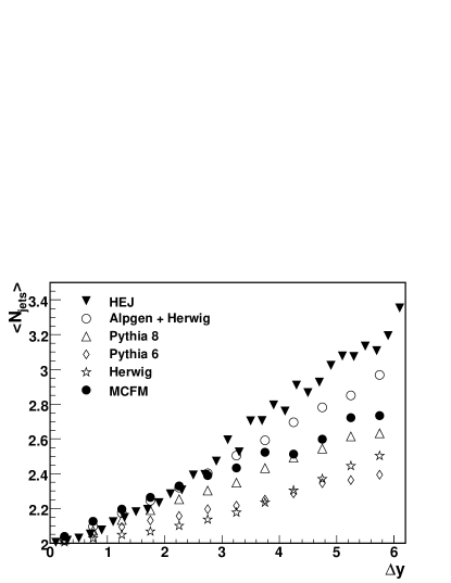
The average number of jets as a function of $\Delta{}y$ is shown in Fig. 27 for the 6 models considered. All the models show a strong correlation between the average number of hard jets and $\Delta y$. We observe that the prediction for the level of hard radiation with increasing $\Delta y$ is smallest for Pythia 6 and Herwig, and highest with HEJ and the PS-matched calculation with Alpgen+HERWIG. The predictions obtained using MCFM or Pythia 8 fall in-between, with MCFM agreeing well with either HEJ or Alpgen+HERWIG out to around 3-4 units of rapidity. Obviously, the maximum number of jets produced in the NLO calculation of W+dijets implemented in MCFM is 3, and as we will see later, the 4-jet rate peaks at around 3-4 units of rapidity. It is therefore perhaps not surprising that the NLO calculation “runs out of steam” in increasing the average jet count at 3-4 units of rapidity. This number coincides well with the general observation of e.g. Ref.[346] that the High Energy resummation produces one hard (40 GeV) jet every (roughly) two units of rapidity span. Therefore one could expect the jet rate predictions obtained in the resummation and the NLO calculation to agree up to 3-4 units of rapidity, where-after the resummation will start producing more than the maximum number of jets allowed in the NLO calculation.

The prediction for the average number of jets vs. the rapidity span is clearly sensitive to scale choices. For MCFM, we used $\mu_{f}\!=\!\mu_{r}\!=\!M_{W}$, in HEJ we used $\mu_{f}\!=\!\mu_{r}\!=\!40$ GeV, while the parton shower predictions used their inherent choices. A systematic study of the uncertainties is clearly desirable.

The average number of jets obtained using MCFM is just two plus the ratio of the (inclusive) 3-jet rate over the inclusive 2-jet rate. This ratio was studied in Ref.[354], but with both the 3-jet rate and the 2-jet rate calculated at both LO and NLO. Both show the same strong correlation.

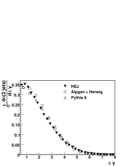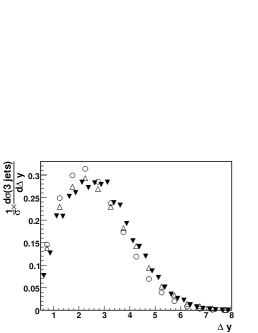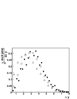(a)	(b)	(c)

Figure 28: Spectrum of the rapidity difference between the forward and the backward jets for (a) at least two, (b) at least three, (c) at least four jets. Results for three generators are reported.

The normalized differential cross-section $\frac{1}{\sigma_{W+n\mathrm{jets}}}\frac{d\sigma_{W+n\mathrm{jets}}}{d\Delta{}y}$, for inclusive production of two, three and four jets is shown in Fig. 28 for Pythia 8, Alpgen+HERWIG and HEJ. We observe that for increasing jet count, the cross-section peaks at an increasingly larger value of $\Delta{}y$ (about 1 unit of rapidity for each extra jet count). This is because of the opening of phase space, and is observed also in the pure tree-level calculations. It is rather surprising how for two and three jets all models shows a similar dependence on $\Delta{}y$. However, for four or more jets clear differences appear. In fact, the spectrum for 4 jets produced with Pythia 8 peaks at the same value of $\Delta y$ as for 3 jets produced with Pythia 8.

Figure 29: Relative exclusive jet rates for three rapidity intervals for different generators.

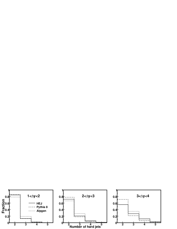
To further investigate the radiation pattern as a funcion of $\Delta{}y$ we concentrated on three bins of $\Delta{}y$ and compared the distribution of the number of jets predicted by the different models, as shown in Fig. 29. It appears that the matched parton shower calculation predicts a larger number of three jets events compared to both the parton shower and the high energy resummation for all rapidity spans, and (unsurprisingly) the pure shower (represented by Pythia 8) has the largest relative weight on exclusive two-jet events. For rapidity spans of more than three, the high energy resummation predicts a significantly larger relative weight on events with four or more jets than does Alpgen+HERWIG or Pythia 8.

16.5 Conclusions

In this contribution we have initiated a comparison of the description of the multi-jet configurations in $W+$jets as obtained using various approximations. Specifically, we have explained why there is a strong correlation between the average number of jets and the rapidity difference between the most forward and most backward jet, and why one can expect differences in the description of this quantity within the generators frequently used for studying LHC physics. We note that the observed differences obtained in the predictions are stable against variations in both the jet energy scale and the parameters used in defining the jets. Specifically, we tried all four combinations with a transverse momentum cut of 30 GeV or 40 GeV, and a parameter of D=0.4 or D=0.7 for the $k_{\perp}$-jet algorithm. We estimate that the differences observed in the predictions are sufficient that 1fb^-1 of $\sqrt{s}=7$ TeV data from the first year of LHC running can discriminate between the models.

The universal behaviour observed in all the models of a strong correlation between the rapidity span and the jet activity is (within the framework of Ref.[339, 340, 341, 342]) universal for all dijet processes. This means that information about jet vetos in e.g. Higgs boson production in association with dijets can be extracted using e.g. W+dijets as studied in this contribution.

17 NNLO QCD EFFECTS ON $\mathrm{H}\rightarrow\mathrm{WW}\rightarrow\ell\nu\ell\nu$ AT HADRON COLLIDERS

17.1 INTRODUCTION

Discovering the Higgs boson is one of the major goals of the hadron colliders Tevatron and LHC. It has been shown that if the Higgs mass lies in the region $m_{\mathrm{H}}\sim 2\times m_{\mathrm{W}}$ the Higgs decay process $\mathrm{H}\to\mathrm{WW}$ serves as the most promising discovery channel. At both the colliders under consideration the main Higgs production process is gluon-fusion. There exists extensive literature about this process and its sensitivity to higher order QCD corrections [311, 312, 313]. In the following we investigate the impact of these higher order corrections in the specific case when the Higgs bosons decays into a pair of W bosons, which further decay into leptons.

17.2 CROSS-SECTIONS AT THE LHC

In this section we present the numbers for the Standard Model (SM) $\mathrm{H}\to\mathrm{WW}\to\ell\nu\ell\nu$ cross-section via gluon-fusion in proton-proton collisions at a center of mass energy of 14 TeV. As an example we choose a Higgs mass of $m_{\mathrm{H}}=165\,\mathrm{GeV}$, where the decay into a pair of W-bosons is dominating. It has been shown that for a Higgs mass around that value this is the most promising discovery channel for the SM Higgs boson at the LHC experiments.

17.2.1 INCLUSIVE CROSS-SECTION

We compute the cross-sections for a center of mass energy of $E_{\mathrm{CM}}=14\,\mathrm{TeV}$ and a Higgs mass of $m_{\mathrm{H}}=165\,\mathrm{GeV}$ using the program FEHiP [355]. The renormalization and factorization scales are varied within $\mu_{\mathrm{R}}=\mu_{\mathrm{F}}\in[m_{\mathrm{H}}/2,2\,m_{\mathrm{H}}]$ to estimate the level of convergence of the perturbative calculation. The numbers, together with the $K$-factors are shown in Tab. 10.

$\sigma_{\mathrm{inc}}\;\;[\mathrm{fb}]$	LO	NLO	NNLO	$K^{\mathrm{NLO}}$	$K^{\mathrm{NNLO}}$
$\mu=m_{\mathrm{H}}/2$	$152.63\pm 0.06$	$270.61\pm 0.25$	$301.23\pm 1.19$	$1.773\pm 0.001$	$1.974\pm 0.008$
$\mu=2\,m_{\mathrm{H}}$	$103.89\pm 0.04$	$199.76\pm 0.17$	$255.06\pm 0.81$	$1.923\pm 0.002$	$2.455\pm 0.008$

Table 10: Inclusive cross sections for $m_{\mathrm{H}}=165\,\mathrm{GeV}$ and $E_{\mathrm{CM}}=14\,\mathrm{TeV}$, at various orders in perturbation theory and for different scale choices.

As expected, the impact of the higher order corrections is rather large. Depending on the scale choice the effects are between $77\%$ and $92\%$ at NLO and between $97\%$ and $145\%$ at NNLO. On the other hand the uncertainty on the cross-sections under variation of the scales are reduced, from $47\%$ at LO to $35\%$ at NLO and $18\%$ at NNLO. This indicates that the perturbative series has not sufficiently converged at NLO and the NNLO corrections have to be taken into account in order to get a reliable cross-section prediction.

17.2.2 IMPACT OF A JET-VETO

Here we demonstrate that applying experimental cuts can have a strong impact on the $K-$factors in Tab. 10. As an example we apply a jet-veto. Such a jet-veto serves to reduce the background arising from top-pair production. Jets are constructed by clustering partons into a jet when they lie within a cone of radius $R=0.4$ and in the pseudo-rapidity range $|\eta|<2.5$. The jet-veto procedure consists of vetoing any event that contains at least one jet with transverse momentum $p_{\mathrm{T}}^{\mathrm{jet}}$ larger than some cut-off value $p_{\mathrm{T}}^{\mathrm{veto}}$. We show the cross-section, as well as the $K$-factors as a function of this cut-off value in Fig. 30.

Figure 30: Cross-section (left) and $K-$factor (right) as a function of the jet-veto cut-off value $p_{\mathrm{T}}^{\mathrm{veto}}$ for a Higgs mass of $m_{\mathrm{H}}=165\,\mathrm{GeV}$.

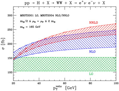
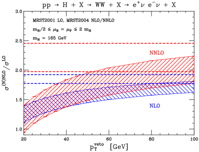
It can be seen how that the (N)NLO cross-sections, and thus the corresponding $K$-factors decrease when lowering the cut-off value $p_{\mathrm{T}}^{\mathrm{veto}}$, while the LO cross-section stays constant. Obviously this can be understood from the fact that at LO there are no partons present in the final state, thus the jet-veto has no impact on the cross-section. As a consequence, $K$-factors close to unity are found, if the jet-veto restricts the phase space strongly enough. In addition, the scale uncertainty of the NNLO results decreases with lower cut-off $p_{\mathrm{T}}^{\mathrm{veto}}$. This can be understood from the fact that the jet-veto eliminates phase space regions were the one(two)-real-radiation diagrams are dominant. These diagrams however are especially sensitive to the variation of the scales. A more detailed study can be found in the dedicated papers [317, 356].

17.3 CROSS-SECTIONS AT THE TEVATRON

In this section we present numbers computed for proton-antiproton collisions at a center of mass energy of $1.96\,\mathrm{TeV}$, as currently produced at the Tevatron collider at Fermilab. Since the performance of simple cut-based analyses is not sufficient to observe or exclude a SM Higgs signal in those experiments, more involved, multi-variate techniques have to be applied. Typical examples for such techniques are Artificial Neural Networks (ANN).

Such techniques have been used in the recent past in order to exclude a SM Higgs boson in the mass range $m_{\mathrm{H}}\in[160\,\mathrm{GeV},170\,\mathrm{GeV}]$ at $95\%$ confidence level in a combined analysis of the two experiments CDF and D0 [357, 358]. A substantial part of the exclusion power of these analyses comes from the decay mode discussed here ($\mathrm{H}\to\mathrm{WW}\to\ell\nu\ell\nu$). Both experiments present numbers for this mode, which allow the exclusion of a Higgs cross-section of about $1.5-1.7$ times the SM cross-section at $95\%$ CL [359, 360, 361].

In what follows we present the numbers for the inclusive cross-section with $m_{\mathrm{H}}=160\,\mathrm{GeV}$, the cross-section after a typical set of selection cuts, and investigate the impact of the effects of the higher order corrections on the efficiencies of such cuts and on typical input variables to ANN analyses, as used by the Tevatron experiments. Further we discuss uncertainties on signal yields when braking up the sample into jet multiplicity bins and finally provide the output of an example ANN. For a more detailed discussion we refer to the dedicated paper [356].

17.3.1 INCLUSIVE CROSS-SECTIONS AND PRE-SELECTION

First we present the numbers for the inclusive cross-section, together with the corresponding $K$-factors. The numbers are again computed using the MRST2004 PDF sets at (N)NLO and MRST2001 PDF set at LO. The uncertainty due to the choice of the renormalization and factorization scales ($\mu:=\mu_{\mathrm{R}}=\mu_{\mathrm{F}}$) are estimated by varying them simultaneously in the range $\mu\in[m_{\mathrm{H}}/2,2\,m_{\mathrm{H}}]$ around the central value $\mu=m_{\mathrm{H}}$. The quoted errors are the residual numerical uncertainty from the MC integration.

$\sigma_{\mathrm{inc}}\;\;[\mathrm{fb}]$	LO	NLO	NNLO	$K^{\mathrm{NLO}}$	$K^{\mathrm{NNLO}}$
$\mu=m_{\mathrm{H}}/2$	$1.998\pm 0.003$	$4.288\pm 0.004$	$5.252\pm 0.016$	$2.149\pm 0.008$	$2.629\pm 0.009$
$\mu=m_{\mathrm{H}}$	$1.398\pm 0.001$	$3.366\pm 0.003$	$4.630\pm 0.010$	$2.412\pm 0.002$	$3.312\pm 0.008$
$\mu=2\,m_{\mathrm{H}}$	$1.004\pm 0.001$	$2.661\pm 0.002$	$4.012\pm 0.007$	$2.651\pm 0.008$	$3.996\pm 0.008$

Table 11: Inclusive cross sections for $m_{\mathrm{H}}=160\,\mathrm{GeV}$ in $\mathrm{p}\bar{\mathrm{p}}$ collisions at $E_{\mathrm{CM}}=1.96\,\mathrm{TeV}$, at various orders in perturbation theory and for different scale choices.

While the uncertainty from the scale variation is reduced when going from LO $\left({}^{+43\%}_{-28\%}\right)$ to NNLO $\left({}^{+13\%}_{-13\%}\right)$, the effect of the higher order corrections is rather large ($\sigma^{\mathrm{NNLO}}\sim 1.4\times\sigma^{\mathrm{NLO}}\sim 3.3\times\sigma^{\mathrm{LO}}$).

We now apply a typical set of pre-selection cuts. Such cuts are needed due to the detector geometry, like the limited coverage in $\eta$, and in order to remove the first substantial part of background events. The cuts we apply here are inspired by the ones applied in the CDF analysis [359], but are not identical to them.

1. Lepton selection: in the CDF experiment, the experimental acceptances for electrons and muons are different. For this study we concentrate on the muon case only. First, one of the final-state leptons has to trigger the event read-out. This ‘trigger lepton’ must have a transverse momentum $p_{\mathrm{T}}>20\,\mathrm{GeV}$. The pseudo-rapidity coverage of the detector for measuring this trigger muon is $|\eta|<0.8$. In order to pass a further lepton selection, a second muon must be found with $p_{\mathrm{T}}>10\,\mathrm{GeV}$ and $|\eta|<1.1$.

   It is worth noting that the differences in the muon and electron cuts are rather geometric, and should not alter the convergence pattern of the perturbative corrections.
   

   1. Two opposite-sign leptons have to be found, fulfilling the requirements discussed above.

   2. Both leptons have to be isolated, i.e. the additional transverse energy in a cone with radius $R=0.4$ around the lepton has to be smaller than 10 % of the lepton transverse momentum.

   3. In order to reduce the background from b resonances, the invariant mass of the lepton pair has to be $m_{\ell\ell}>16\,\mathrm{GeV}$.
      

2. The missing transverse energy (MET) is defined as the vectorial sum of the transverse momenta of the two neutrinos. Then we can define the variable $\mathrm{MET}^{*}$ as

   $$\mathrm{MET}^{*}=\left\{\begin{array}[]{l}\mathrm{MET}\;\;\;\;\;\;\;\;\;\;\;\;,\;\phi\geq\pi/2\\ \mathrm{MET}\times\sin{\phi}\;,\;\phi<\pi/2\end{array}\right.,$$ (62)

   where $\phi$ is the angle in the transverse plane between MET and the nearest charged lepton or jet. We require $\mathrm{MET}^{*}>25$ GeV, which suppresses the background from Drell-Yan lepton pairs and removes contributions from mismeasured leptons or jets.

3. In order to suppress the $t{\bar{t}}$ background, we apply a veto on the number of jets in the event. Jets are found using the $k_{\mathrm{T}}$-algorithm with parameter $R=0.4$. A jet must have $p_{\mathrm{T}}>15\,\mathrm{GeV}$ and $|\eta|<3.0$. Events are only accepted if there is no more than one such jet.

$\sigma_{\mathrm{acc}}\;\;[\mathrm{fb}]$	LO	NLO	NNLO	$K^{\mathrm{NLO}}$	$K^{\mathrm{NNLO}}$
$\mu=m_{\mathrm{H}}/2$	$0.750\pm 0.001$	$1.410\pm 0.003$	$1.459\pm 0.003$	$1.880\pm 0.005$	$1.915\pm 0.025$
$\mu=m_{\mathrm{H}}$	$0.525\pm 0.001$	$1.129\pm 0.003$	$1.383\pm 0.004$	$2.150\pm 0.007$	$2.594\pm 0.052$
$\mu=2\,m_{\mathrm{H}}$	$0.379\pm 0.001$	$0.903\pm 0.002$	$1.242\pm 0.001$	$2.383\pm 0.008$	$3.261\pm 0.048$

Table 12: Accepted cross sections and $K$-factors after the application of all the selection cuts for $m_{\mathrm{H}}=160\,\mathrm{GeV}$ in $\mathrm{p}\bar{\mathrm{p}}$ collisions at $E_{\mathrm{CM}}=1.96\,\mathrm{TeV}$.

The numbers and the $K$-factors after applying these cuts are shown in Tab. 12. The impact of QCD radiative corrections is significantly reduced when selection cuts are applied. For $\mu=m_{\mathrm{H}}$ the NLO and NNLO $K$-factors are reduced by $11\%$ and $22\%$, respectively. As a consequence, also the acceptance is reduced, since it is defined as the ratio of the cross-section after cuts over the inclusive cross section. At LO about $\sim 37.5\%$ of the events are accepted. At NLO, the efficiency drops to $33\%-34\%$ and at NNLO to $28\%-31\%$, depending on the scale choice.

Figure 31: Kinematic distributions obtained at LO, NLO and NNLO in perturbative QCD. Shown are the invariant mass of the two charged leptons ($m_{\ell\ell}$) and the azimuthal separation of the two charged leptons in the transverse plane ($\phi_{\ell\ell}$).

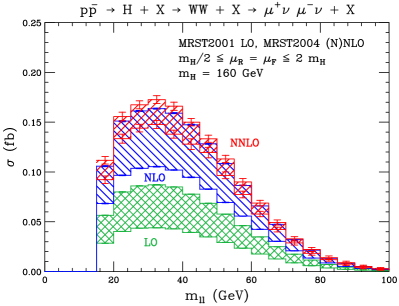
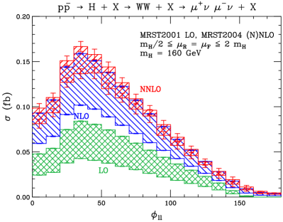
In Fig. 31 we show kinematic distributions at different orders in perturbation theory after applying the cuts described above. Distributions like this are typical input variables for multi-variate analyses such as artificial neural networks (ANN). On the left the invariant mass of the charged lepton pair is shown ($m_{\ell\ell}$), on the right the azimuthal angle between these leptons ($\phi_{\ell\ell}$). The uncertainty bands show again the variation of the distributions under the variation of the ren. and fac. scales $\mu$. The plots show a stable behavior with respect to both, the scale variation and the addition of higher order corrections. This is no surprise, since the leptonic final state variables are not expected to be very sensitive to the higher order QCD corrections. This picture changes when more involved, hadronic variables are under consideration. When such variables (like the number of jets) are used, e.g. as input to a ANN, care must be taken that these variables, and especially the uncertainties on them are well understood and under control. This is discussed in some detail in the next section.

17.3.2 JET-MULTIPLICITY

In an experimental analysis it might seem beneficial to divide the experimental candidate data into different sub-samples, distinguishable by the number of jets in the events. A possible division is the one into the mutually exclusive ’0-jet’, ’1-jet’ and ’$\geq 2$-jets’ sub-samples. Further, for each sub-sample, a dedicated analysis can be performed, benefiting from the different kinematic behavior, not only of the signal, but especially for the background events (as an example, the ’0-jet’ sub-sample suffers much less from contamination by $\mathrm{t}\bar{\mathrm{t}}$ events). Such a strategy is e.g. pursued by the CDF analysis [360]. It has to be pointed out, that, if a jet is required in all events, the ${\cal O}(\alpha_{s}^{4})$ calculation includes matrix elements through NLO only. If two jets are required, only LO matrix-elements are taken into account. More importantly, we find it inconsistent to use the theoretical uncertainty from the inclusive NNLO gluon fusion cross-section as the uncertainty of the samples with defined jet multiplicities other than zero.

This is illustrated in the example below. We divide the signal cross-section into the three jet-multiplicity bins described above, where jets are defined using a $k_{\mathrm{T}}$-algorithm, and a jet is identified as such when it has a minimal $p_{\mathrm{T}}$ of 15 GeV and lies in the detector region $|\eta|<2$. We now compute the cross-sections varying the ren. and fac. scales in the usual interval, using either NNLO, NLO or LO parton density functions and $\alpha_{s}$ evolution from the MSTW2008 fit. The resulting numbers are shown in Tab. 13.

$\sigma\;\;[\mathrm{fb}]$	LO (pdfs, $\alpha_{s}$)	NLO (pdfs, $\alpha_{s}$)	NNLO (pdfs, $\alpha_{s}$)
0-jet	$3.452^{+7\%}_{-10\%}$	$2.883^{+4\%}_{-9\%}$	$2.707^{+5\%}_{-9\%}$
1-jet	$1.752^{+30\%}_{-26\%}$	$1.280^{+24\%}_{-23\%}$	$1.165^{+24\%}_{-22\%}$
$\geq 2$-jets	$0.336^{+91\%}_{-44\%}$	$0.221^{+81\%}_{-42\%}$	$0.196^{+78\%}_{-41\%}$

Table 13: Inclusive cross-sections in the different jet-multiplicity bins.

From the numbers in Tab. 13 it can be seen that about 66.5% of the events contain no jets, 28.6% contain 1 jet and only 4.9% contain at least 2 jets. From the scale uncertainties listed in the table, the total scale uncertainty on the expected signal yield can be reconstructed as

$$\frac{\Delta N_{\mathrm{inc}}}{N_{\mathrm{inc}}}=66.5\%\cdot\left({}^{+5\%}_{-9\%}\right)+28.6\%\cdot\left({}^{+24\%}_{-22\%}\right)+4.9\%\cdot\left({}^{+78\%}_{-41\%}\right)=\left({}^{+14.0\%}_{-14.3\%}\right),$$ (63)

which agrees well with the $\sim\pm 13\%$ uncertainty retrieved in the previous section. The application of different selection cuts in the three jet-multiplicity bins leads to a theoretical error estimate for the total signal yield which is different from the value for the inclusive NNLO cross-section. To illustrate this, we assume that after applying further selection cuts, 60% of the events belong to the ’0-jet’ bin, 29% to the ’1-jet’ bin and 11% to the ’$\geq 2$-jet’ bin. Recomputing the uncertainty on the total signal yield along the lines of eq. 63 results in

$$\frac{\Delta N_{\mathrm{inc}}}{N_{\mathrm{inc}}}=66\%\cdot\left({}^{+5\%}_{-9\%}\right)+29\%\cdot\left({}^{+24\%}_{-22\%}\right)+11\%\cdot\left({}^{+78\%}_{-41\%}\right)=\left({}^{+18.5\%}_{-16.3\%}\right),$$ (64)

which is substantially larger then the errors on the inclusive cross-sections. Moreover, a more consistent approach would be to estimate the number of ’1-jet’ (’$\geq 2$-jets’) events using NLO (LO) PDFs and $\alpha_{s}$ evolution correspondingly. This would lead to

$$\frac{\Delta N_{\mathrm{inc}}}{N_{\mathrm{inc}}}=66\%\cdot\left({}^{+5\%}_{-9\%}\right)+29\%\cdot\left({}^{+24\%}_{-23\%}\right)+11\%\cdot\left({}^{+91\%}_{-44\%}\right)=\left({}^{+20.0\%}_{-16.9\%}\right).$$ (65)

This demonstrates, that the theoretical uncertainty on the number of signal events for different jet-multiplicities should not be estimated collectively from the scale variation of the total cross-section.

17.3.3 ARTIFICIAL NEURAL NETWORK

As a final result we present the fixed order prediction for an example ANN. To train the ANN we have used events generated with PYTHIA8 [352], for the signal process and the background processes $\mathrm{pp}\to\mathrm{WW}$ and $\mathrm{pp}\to\mathrm{t}\bar{\mathrm{t}}$. After this training, we compute the neural-net output variable at different orders of perturbation theory and under the variation of the scales. Obviously this ANN should not be understood as a full fletched analysis. In a real analysis, there a many more background processes that need to be considered, in addition we neglect any detector effects.

Figure 32: ANN output obtained at LO, NLO and NNLO in perturbative QCD. The bands correspond to the variation of the ren. and fac. scales simultaneously in the range $\mu\in[m_{\mathrm{H}}/2,2\,m_{\mathrm{H}}]$.

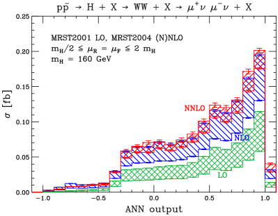
The resulting plots can be seen in Fig. 32. As expected, the bulk of the Higgs cross-section falls into the high-score bins of the ANN output. In addition, the higher order corrections show a stable behavior within the full range of the output variable. This is not surprising, since only ’well-behaved’, i.e. leptonic final state variables were used as input to the ANN. However, this does not guarantee that any ANN follows this stable behavior. Especially when variables are used, that are very sensitive to the inclusion of higher order corrections (e.g. hadronic variables) care must be taken. The uncertainty under variation of the scales can be increased in specific regions of the ANN output, depending on the region of phase-space that is selected by the ANN variable.

CONCLUSIONS

We have presented cross-sections for the process $\mathrm{H}\to\mathrm{WW}\to\ell\nu\ell\nu$ for proton-(anti)-proton collisions at the LHC ($E_{\mathrm{CM}}=14\,\mathrm{TeV}$) and the Tevatron ($E_{\mathrm{CM}}=1.96\,\mathrm{TeV}$) colliders. We have obtained predictions at different orders in perturbation theroy, from LO up to NNLO, and discussed the impact of these higher order corrections.

As expected the corrections are large, reaching $\sim 300\%$ in certain cases. However, it turns out that the $K$-factors depend on the selection cuts that are applied. In the special case of applying a jet-veto the LO to NNLO $K$-factor can decrease to a value as low as $~{}1$. Further we discussed the uncertainties on the cross-section arising from varying the ren. and fac. scales. It was found that in general these decrease when including higher order diagrams in the calculations. We also point out that care has to be taken when dividing the sample into different jet-multiplicity bins. In that case, the uncertainty from the inclusive cross-section does not describe correctly the uncertainty on the cross-sections in the various jet-multiplicity bins.

Finally, for the first time we have computed a ANN output variable at NNLO. It turned out that the higher order corrections show a smooth behavior in our toy ANN, however, when creating a ANN care should be taken in the choice of the input variables to the ANN. We anticipate, without proof, that the ANN behavior will be smooth as long as all the input variables show a smooth behavior. This is typically the case for leptonic final state variables, but not guaranteed for hadronic variables.

18 DETERMINATION OF THE STRONG COUPLING CONSTANT BASED ON NNLO+NLLA RESULTS FOR HADRONIC EVENT SHAPES AND A STUDY OF HADRONISATION CORRECTIONS

18.1 INTRODUCTION

Event-shape observables describe topological properties of hadronic final states without the need to define jets, quantifying the structure of an event by a single measure. This class of observables is also interesting because it shows a rather strong sensitivity to hadronisation effects, at least in phase-space regions characterised by soft and collinear gluon radiation, which correspond to certain limits for each event-shape variable.

Event-shape distributions in $\mathrm{e^{+}e^{-}}$ annihilation have been measured with high accuracy by a number of experiments, most of them at LEP at centre-of-mass energies between 91 and 206 GeV [362, 363, 364, 365, 366, 367, 368, 369, 370, 371, 372, 373, 374, 375, 376]. Mean values and higher moments also have been measured by several experiments, most extensively by JADE [377, 378] and OPAL [368].

For a long time, the theoretical state-of-the-art description of event-shape distributions over the full kinematic range was based on the matching of the next-to-leading-logarithmic approximation (NLLA)
[379] onto the fixed next-to-leading order (NLO) calculation [285, 380, 381]. Recently, NNLO results for event-shape distributions became available [236, 235, 240] and lead to the first determination of the strong coupling constant using NNLO predictions for hadronic event shapes in $\mathrm{e}^{+}\mathrm{e}^{-}$ annihilations [382]. Soon after, the matching of the resummed result in the next-to-leading-logarithmic approximation onto the NNLO calculation has been performed [383] in the so-called $\ln\,R$-matching scheme [379]. Based on these results, a determination of the strong coupling constant using matched NNLO+NLLA predictions for hadronic event shapes has been carried out [384], together with a detailed investigation of hadronisation corrections. Next-to-leading order electroweak corrections to event-shape distributions in $e^{+}e^{-}$ annihilation were also computed very recently [385].

A similar NNLO+NLLA study based on JADE data was done in [386], while other NNLO determinations of $\alpha_{s}(M_{Z})$ based on only the thrust distribution were presented in [387, 388].

Apart from distributions of event-shape observables, one can also study mean values and higher moments, which are now available at NNLO accuracy [238, 241]. Moments are particularly attractive in view of studying non-perturbative hadronisation corrections to event shapes. In ref. [389], NNLO perturbative QCD predictions have been combined with non-perturbative power corrections in a dispersive model [390, 391, 392, 393]. The resulting theoretical expressions have been compared to experimental data from JADE and OPAL, and new values for both $\alpha_{s}(M_{Z})$ and $\alpha_{0}$, the effective coupling in the non-perturbative regime, have been determined.

The two approaches – estimating the hadronisation corrections by general purpose Monte Carlo programs or modelling power corrections analytically – shed light on the subject of hadronisation corrections from two different sides and lead to some interesting insights which will be summarised in the following.

18.2 THEORETICAL FRAMEWORK

We have studied the six event-shape observables thrust $T$ [394] (respectively $\tau=1-T$), heavy jet mass $M_{H}$ [395], wide and total jet broadening $B_{W}$ and $B_{T}$ [396], $C$-parameter [397, 398] and the two-to-three-jet transition parameter in the Durham algorithm, $Y_{3}$ [399, 400]. The definitions of these variables, which we will denote collectively as $y$ in the following, are summarised e.g. in [235].

18.2.1 event-shape distributions

The fixed-order QCD description of event-shape distributions starts from the perturbative expansion

$$\frac{1}{\sigma_{0}}\,\frac{{\rm d}\sigma}{{\rm d}y}(y,Q,\mu) = \bar{\alpha}_{s}(\mu)\frac{{\rm d}{A}}{{\rm d}y}(y)+\bar{\alpha}_{s}^{2}(\mu)\frac{{\rm d}{B}}{{\rm d}y}(y,x_{\mu})+\bar{\alpha}_{s}^{3}(\mu)\frac{{\rm d}{C}}{{\rm d}y}(y,x_{\mu})+{\cal O}(\bar{\alpha}_{s}^{4})\;,$$ (66)

where

$$\bar{\alpha}_{s}=\frac{\alpha_{s}}{2\pi}\;,\qquad x_{\mu}=\frac{\mu}{Q}\;,$$

and where $A$, $B$ and $C$ are the perturbatively calculated coefficients [235] at LO, NLO and NNLO.

All coefficients are normalised to the tree-level cross section $\sigma_{0}$ for $e^{+}e^{-}\rightarrow q\bar{q}$. For massless quarks, this normalisation cancels all electroweak coupling factors, and the dependence of (66) on the collision energy is only through $\alpha_{s}$ and $x_{\mu}$. Predictions for the experimentally measured event-shape distributions are then obtained by normalising to $\sigma_{{\rm had}}$ as

$$\frac{1}{\sigma_{{\rm had}}}\,\frac{{\rm d}\sigma}{{\rm d}y}(y,Q,\mu)=\frac{\sigma_{0}}{\sigma_{{\rm had}}(Q,\mu)}\,\frac{1}{\sigma_{0}}\,\frac{{\rm d}\sigma}{{\rm d}y}(y,Q,\mu)\;.$$ (67)

In all expressions, the scale dependence of $\alpha_{s}$ is determined according to the three-loop running:

$$\alpha_{s}(\mu^{2})=\frac{2\pi}{\beta_{0}L}\left(1-\frac{\beta_{1}}{\beta_{0}^{2}}\,\frac{\ln L}{L}+\frac{1}{\beta_{0}^{2}L^{2}}\,\left(\frac{\beta_{1}^{2}}{\beta_{0}^{2}}\left(\ln^{2}L-\ln L-1\right)+\frac{\beta_{2}}{\beta_{0}}\right)\right)\;,$$ (68)

where $L=2\,\ln(\mu/\Lambda_{\overline{{\rm MS}}}^{(N_{F})})$ and $\beta_{i}$ are the $\overline{{\rm MS}}$-scheme coefficients listed e.g. in [235].

We take into account bottom mass effects by retaining the massless $N_{F}=5$ expressions and adding the difference between the massless and massive LO and NLO coefficients $A$ and $B$ [401, 402, 403, 404], where a pole b-quark mass of $m_{\rm b}$ = 4.5 GeV was used.

In the limit $y\to 0$ one observes that the perturbative contribution of order $\alpha_{s}^{n}$ to the cross section diverges like $\alpha_{s}^{n}L^{2n}$, with $L=-\ln\,y$ ($L=-\ln\,(y/6)$ for $y=C$). This leading logarithmic (LL) behaviour is due to multiple soft gluon emission at higher orders, and the LL coefficients exponentiate, such that they can be resummed to all orders. For the event-shape observables considered here, and assuming massless quarks, the next-to-leading logarithmic (NLL) corrections can also be resummed to all orders in the coupling constant.

In order to obtain a reliable description of the event-shape distributions over a wide range in $y$, it is mandatory to combine fixed order and resummed predictions. However, in order to avoid the double counting of terms common to both, the two predictions have to be matched onto each other. A number of different matching procedures have been proposed in the literature, see e.g. Ref. [405] for a review. The most commonly used procedure is the so-called $\ln\,R$-matching [379], which we used in two different variants for our study on $\alpha_{s}$ [384]. For more details about the NLLA+NNLO matching we refer the reader to Ref. [383].

18.2.2 Moments of event-shape observables

The $n$th moment of an event-shape observable $y$ is defined by

$$\langle y^{n}\rangle=\frac{1}{\sigma_{\rm{had}}}\,\int_{0}^{y_{\rm{max}}}y^{n}\frac{{\rm d}\sigma}{{\rm d}y}{\rm d}y\;,$$ (69)

where $y_{\mathrm{max}}$ is the kinematically allowed upper limit of the observable. For moments of event shapes, one expects the hadronisation corrections to be additive, such that they can be divided into a perturbative and a non-perturbative contribution,

$$\langle y^{n}\rangle=\langle y^{n}\rangle_{\rm{pt}}+\langle y^{n}\rangle_{\rm{np}}\;,$$ (70)

where the non-perturbative contribution accounts for hadronisation effects.

In ref. [389], the dispersive model derived in Refs. [390, 391, 392, 393] has been used to estimate hadronisation corrections to event-shape moments by calculating analytical predictions for power corrections. It introduces only a single new parameter $\alpha_{0}$, which can be interpreted as the average strong coupling in the non-perturbative region:

$$\frac{1}{\mu_{I}}\int_{0}^{\mu_{I}}dQ\,\alpha_{\rm{eff}}(Q^{2})=\alpha_{0}(\mu_{I})\;,$$ (71)

where below the IR cutoff $\mu_{I}$ the strong coupling is replaced by an effective coupling. This dispersive model for the strong coupling leads to a shift in the distributions

$$\frac{{\rm d}\sigma}{{\rm d}y}(y)=\frac{{\rm d}\sigma_{\rm{pt}}}{{\rm d}y}\,(y-a_{y}\,P)\;,$$ (72)

where the numerical factor $a_{y}$ depends on the event shape, while ${P}$ is believed to be universal and scales with the centre-of-mass energy like $\mu_{I}/Q$. Insertion of eq. (72) into the definition of the moments leads to

$$\langle y^{n}\rangle = \int^{y_{\mathrm{max}}-a_{y}P}_{-a_{y}P}\mathrm{d}y\,(y+a_{y}P)^{n}\frac{1}{\sigma_{\mathrm{tot}}}\frac{\mathrm{d}\sigma_{\mathrm{pt}}}{\mathrm{d}y}(y)$$ (73)

$$\approx \int^{y_{\mathrm{max}}}_{0}\mathrm{d}y\,(y+a_{y}P)^{n}\frac{1}{\sigma_{\mathrm{tot}}}\frac{\mathrm{d}\sigma_{\mathrm{pt}}}{\mathrm{d}y}(y)\;.$$

From this expression one can extract the non-perturbative predictions for the moments of $y$. To combine the dispersive model with the perturbative prediction at NNLO QCD, the analytical expressions have been extended [389] to compensate for all scale-dependent terms at this order.

18.3 DETERMINATION OF $\alpha_{s}$ AND $\alpha_{0}$

18.3.1 $\alpha_{s}$ from distributions of hadronic event shapes

We have used the six event-shape observables listed in section 18.2 for our fits. The measurements we use have been carried out by the ALEPH collaboration [362] at eight different centre-of-mass energies between 91.2 and 206 GeV. The event-shape distributions were obtained from the reconstructed momenta and energies of charged and neutral particles. The measurements have been corrected for detector effects, i.e. the final distributions correspond to the so-called particle (or hadron) level. In addition, at LEP2 energies above the Z peak they were corrected for initial-state radiation effects. At energies above 133 GeV, backgrounds from 4-fermion processes, mainly from W-pair production and also ZZ and Z$\gamma^{*}$, were subtracted following the procedure given in [362]. The experimental uncertainties were estimated by varying event and particle selection cuts. They are below 1% at LEP1 and slightly larger at LEP2.

The perturbative QCD prediction is corrected for hadronisation and resonance decays by means of a transition matrix, which is computed with the Monte Carlo generators PYTHIA [406], HERWIG [407] and ARIADNE [408], all tuned to global hadronic observables at $M_{Z}$ [409]. The parton level is defined by the quarks and gluons present at the end of the parton shower in PYTHIA and HERWIG and the partons resulting from the colour dipole radiation in ARIADNE. Corrected measurements of event-shape distributions are compared to the theoretical calculation at particle level. For a detailed description of the determination and treatment of experimental systematic uncertainties we refer to Refs. [362, 382].

We also made studies using the NLO+LL event generator HERWIG++ [410], which will be described in more detail below.

The value of $\alpha_{s}$ is determined at each energy using a binned least-squares fit. The fit programs of Ref. [382] have been extended to incorporate the NNLO+NLLA calculations. Combining the results for six event-shape variables and eight LEP1/LEP2 centre-of-mass energies, we obtain

$\alpha_{s}(M_{Z})=0.1224\;\pm\;0.0009\,\mathrm{(stat)}\;\pm\;0.0009\,\mathrm{(exp)}\;\pm\;0.0012\,\mathrm{(had)}\;\pm\;0.0035\,\mathrm{(theo)}\;.$

The fitted values of the coupling constant as found from event-shape variables calculated at various orders are shown in Fig. 33.

Figure 33: The measurements of the strong coupling constant $\alpha_{s}$ for the six event shapes, at $\sqrt{s}=M_{Z}$, when using QCD predictions at different approximations in perturbation theory. The shaded area corresponds to the total uncertainty.

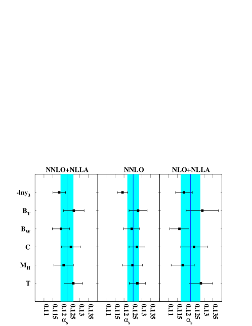
Comparing our results to both the fit using purely fixed-order NNLO predictions [382] and the fits based on earlier NLLA+NLO calculations [362], we make the following observations:

• The central value is slightly lower than the central value of 0.1228 obtained from fixed-order NNLO only, and slightly larger than the NLO+NLLA results. The fact that the central value is almost identical to the purely fixed-order NNLO result could be anticipated from the findings in Ref. [383]. There it is shown that in the three-jet region, which provides the bulk of the fit range, the matched NLLA+NNLO prediction is very close to the fixed-order NNLO calculation.

• The dominant theoretical uncertainty on $\alpha_{s}(M_{Z})$, as estimated from scale variations, is reduced by 20% compared to NLO+NLLA. However, compared to the fit based on purely fixed-order NNLO predictions, the perturbative uncertainty is increased in the NNLO+NLLA fit. The reason is that in the two-jet region the NLLA+NLO and NLLA+NNLO predictions agree by construction, because the matching suppresses any fixed order terms. Therefore, the renormalisation scale uncertainty is dominated by the next-to-leading-logarithmic approximation in this region, which results in a larger overall scale uncertainty in the $\alpha_{s}$ fit.

• As already observed for the fixed-order NNLO results, the scatter among the values of $\alpha_{s}(M_{Z})$ extracted from the six different event-shape variables is substantially reduced compared to the NLO+NLLA case.

• The matching of NLLA+NNLO introduces a mismatch in the cancellation of renormalisation scale logarithms, since the NNLO expansion fully compensates the renormalisation scale dependence up to two loops, while NLLA only compensates it up to one loop. In order to assess the impact of this mismatch, we have introduced the $\ln R(\mu)$ matching scheme [384], which retains the two-loop renormalisation terms in the resummed expressions and the matching coefficients. In this scheme, a substantial reduction of the perturbative uncertainty from $\pm 0.0035$ (obtained in the default $\ln R$-scheme) to $\pm 0.0022$ is observed, which might indicate the size of the ultimately reachable precision for a complete NNLO+NNLLA calculation. Although both schemes are in principle on the same theoretical footing, it is the more conservative error estimate obtained in the $\ln R$-scheme which should be taken as the nominal value, since it measures the potential impact of the yet uncalculated finite NNLLA-terms.

• Bottom quark mass effects, which are numerically significant mainly at the LEP1 energy, were included through to NLO. Compared to a purely massless evaluation of the distributions, the inclusion of these mass effects enhances $\alpha_{s}(M_{Z})$ by 0.8%.

Hadronisation corrections from LL+NLO event generators

In recent years large efforts went into the development of modern Monte Carlo event generators which include in part NLO corrections matched to parton showers at leading logarithmic accuracy (LL) for various processes. Here we use HERWIG++ [410, 411] version 2.3 for our investigations. Several schemes for the implementation of NLO corrections are available [412, 413, 414]. We studied the MCNLO [412] and POWHEG [413] schemes.

We compared the prediction for the event-shape distributions of HERWIG++ to both the high precision data at LEP1 from ALEPH and the predictions from the legacy generators PYTHIA, HERWIG and ARIADNE. We recall that the latter have all been tuned to the same global QCD observables measured by ALEPH [409] at LEP1, which included event-shape variables similar to the ones analysed here. To investigate the origin of the observed differences between the generators, we decided to consider the parton-level predictions and the hadronisation corrections separately. Discussing the full details of our study is beyond the scope of this note; here we only mention some of our observations. HERWIG++ with POWHEG yields a similar shape as the legacy programs, but differs in the normalisation. The other HERWIG++ predictions differ most notably in shape from the former. The fit quality of HERWIG++ with POWHEG is similar to the outcome of the legacy generators. Given the similar shape but different normalisation of HERWIG++ with POWHEG, the resulting values of $\alpha_{s}$ are significantly lower, overall by 3 $\%$. For further details we refer to Ref. [384].

From the study of hadronisation corrections we make the following important observation. It appears that there are two “classes” of variables. The first class contains thrust, C-parameter and total jet broadening, while the second class consists of the heavy jet mass, wide jet broadening and the two-to-three-jet transition parameter $Y_{3}$. For the first class, using the standard hadronisation corrections from PYTHIA, we obtain $\alpha_{s}(M_{Z})$ values around $0.125-0.127$, some $5\%$ higher than those found from the second class of variables. In a study of higher moments of event shapes [238], indications were found that variables from the first class still suffer from sizable missing higher order corrections, whereas the second class of observables have a better perturbative stability. In Ref. [384], we observed that this first class of variables gives a parton level prediction with PYTHIA, which is about $10\%$ higher than the NNLO+NLLA prediction. The PYTHIA result is obtained with tuned parameters, where the tuning to data had been performed at the hadron level. This tuning results in a rather large effective coupling in the parton shower, which might partly explain the larger parton level prediction of PYTHIA. As the tuning has been performed at hadron level, this implies that the hadronisation corrections come out to be smaller than what would have been found by tuning a hypothetical Monte Carlo prediction with a parton level corresponding to the NNLO+NLLA prediction. This means that the PYTHIA hadronisation corrections, applied in the $\alpha_{s}$ fit, might be too small, resulting in a larger $\alpha_{s}(M_{Z})$ value. Since up to now the hadronisation uncertainties have been estimated from the differences of parton shower based models, tuned to the data, it is likely that for these event shapes the uncertainties were underestimated, missing a possible systematic shift. Such problems do not appear to exist for the second class of variables.

We would like to mention that a determination of $\alpha_{s}$ based on 3-jet rates calculated at NNLO accuracy also has been performed recently [415], with the result $\alpha_{s}(M_{Z})=0.1175\pm 0.0020\,(\mathrm{exp})\pm 0.0015\,(\mathrm{theo})$, which is also lower than the one obtained from fits to distributions of event shapes.

18.3.2 $\alpha_{s}$ and $\alpha_{0}$ from moments of hadronic event shapes

Now we turn to analytical models to estimate hadronisation corrections. The expressions derived in [389] match the dispersive model with the perturbative prediction at NNLO QCD. Comparing these expressions with experimental data on event-shape moments, a combined determination of the perturbative strong coupling constant $\alpha_{s}$ and the non-perturbative parameter $\alpha_{0}$ has been performed [389], based on data from the JADE and OPAL experiments [378]. The data consist of 18 points at centre-of-mass energies between 14.0 and 206.6 GeV for the first five moments of $T$, $C$, $Y_{3}$, $M_{H}$, $B_{W}$ and $B_{T}$, and have been taken from [416]. For each moment the NLO as well as the NNLO prediction was fitted with $\alpha_{s}(M_{Z})$ and $\alpha_{0}$ as fit parameters, except for the moments of $Y_{3}$, which have no power correction and thus are independent of $\alpha_{0}$.

Compared to previous results at NLO, inclusion of NNLO effects results in a considerably improved consistency in the parameters determined from different shape variables, and in a substantial reduction of the error on $\alpha_{s}$.

We further observe that the theoretical error on the extraction of $\alpha_{S}(M_{Z})$ from $\rho$, $Y_{3}$ and $B_{W}$ is considerably smaller than from $\tau$, $C$ and $B_{T}$. As mentioned above and discussed in detail in [238], the moments of the former three shape variables receive moderate NNLO corrections for all $n$, while the NNLO corrections for the latter three are large already for $n=1$ and increase with $n$. Consequently, the theoretical description of the moments of $\rho$, $Y_{3}$ and $B_{W}$ displays a higher perturbative stability, which is reflected in the smaller theoretical uncertainty on $\alpha_{S}(M_{Z})$ derived from those variables.

In a second step, we combine the $\alpha_{s}(M_{Z})$ and $\alpha_{0}$ measurements obtained from different event-shape variables. Taking the weighted mean over all values except $B_{W}$ and $B_{T}$, we obtain at NNLO:

$$\alpha_{s}(M_{Z}) =0.1153\pm 0.0017(\mathrm{exp})\pm 0.0023(\mathrm{th}),$$

$$\alpha_{0} =0.5132\pm 0.0115(\mathrm{exp})\pm 0.0381(\mathrm{th})\,,$$ (74)

The moments of $B_{W}$ and $B_{T}$ have been excluded here since their theoretical description requires an additional contribution to the non-perturbative coefficient $P$ (see eq. (72)) which is not available consistently to NNLO.

To illustrate the improvement due to the inclusion of the NNLO corrections, we also quote the corresponding NLO results. Based on $\tau$, $C$, $\rho$ and $Y_{3}$, we obtain:

$$\alpha^{{\rm NLO}}_{s}(M_{Z}) =0.1200\pm 0.0021(\mathrm{exp})\pm 0.0062(\mathrm{th}),$$

$$\alpha^{{\rm NLO}}_{0} =0.4957\pm 0.0118(\mathrm{exp})\pm 0.0393(\mathrm{th})\,,$$

We compare the NLO and NNLO combinations in Figure 34. It can be seen very clearly that the measurements obtained from the different variables are consistent with each other within errors. The average of $\alpha_{s}(M_{Z})$ is dominated by the measurements based on $\rho$ and $Y_{3}$, which have the smallest theoretical uncertainties. From NLO to NNLO, the error on $\alpha_{s}(M_{Z})$ is reduced by a factor of two. Analysing the different sources of the systematical errors, we observe that the error on $\alpha_{s}(M_{Z})$ is clearly dominated by the $x_{\mu}$ variation, while the largest contribution to the error on $\alpha_{0}$ comes from the uncertainty on the Milan factor ${\cal M}$ [392]. Since this uncertainty has not been improved in the current study, it is understandable that the systematic error on $\alpha_{0}$ remains unchanged.

Figure 34: Error bands at NLO and NNLO for combinations of values for $\alpha_{s}$ and $\alpha_{0}$ obtained from fits to moments of different event shapes. The error on $\alpha_{s}$ is dominated by scale uncertainties, while the largest contribution to the error on $\alpha_{0}$ comes from the uncertainty on the Milan factor.

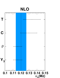
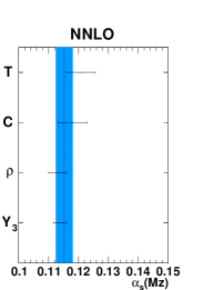
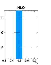
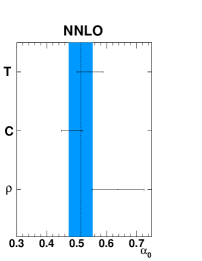
To quantify the difference of the dispersive model to hadronisation corrections from the legacy generators, we analysed the moments of (1-T) with hadronisation corrections from PYTHIA. As a result, we obtained fit results for $\alpha_{s}(M_{\mathrm{Z}})$ which are typically 4% higher than by using the dispersive model, with a slightly worse quality of the fit. Comparing perturbative and non-perturbative contributions at $\sqrt{s}=M_{{\mathrm{Z}}}$, we observed that PYTHIA hadronisation corrections amount to less than half the power corrections obtained in the dispersive model, thereby explaining the tendency towards a larger value of $\alpha_{s}(M_{\mathrm{Z}})$, since the missing numerical magnitude of the power corrections must be compensated by a larger perturbative contribution.

CONCLUSIONS

We have compared determinations of the strong coupling constant based on hadronic event shapes measured at LEP using two different approaches:

1. a fit of perturbative QCD results at next-to-next-to-leading order (NNLO), matched to resummation in the next-to-leading-logarithmic approximation (NLLA), to ALEPH data where the hadronisation corrections have been estimated using Monte Carlo event generators

2. a fit of perturbative QCD results at NNLO matched to non-perturbative power corrections in the dispersive model, providing analytical parametrisations of hadronisation corrections, to JADE and OPAL data.

We find that the second approach results in a considerably lower value of $\alpha_{s}(M_{Z})$ than the first one.

We conclude that apparently there are two “classes” of event-shape variables, the first class containing thrust, C-parameter and total jet broadening, the second class containing heavy jet mass, wide jet broadening and the two-to-three-jet transition parameter $Y_{3}$. Comparing parton level and hadron level predictions from PYTHIA, this first class of variables gives a parton level prediction which is about $10\%$ higher than the NNLO+NLLA prediction, where the PYTHIA curve has been obtained with tuned parameters, the tuning to data being performed at the hadron level. This tuning results in a rather large effective coupling in the parton shower, such that the parton level prediction of PYTHIA turns out large. This may imply that the hadronisation corrections come out to be too small for these variables, resulting in a larger $\alpha_{s}(M_{Z})$ value. This hypothesis is corroborated by the fact that the theoretical description of the moments of the variables thrust, C-parameter and total jet broadening displays a lower perturbative stability.

For the moments of (1-T), we found that the legacy generators predict power corrections which are less than half of what is obtained in the dispersive model. The large numerical discrepancy between analytical power corrections and the estimate of hadronisation effects from the legacy generators suggests to revisit the impact of hadronisation corrections on precision QCD observables.

ACKNOWLEDGEMENTS

This research was supported in part by the Swiss National Science Foundation (SNF) under contracts PP0022-118864 and 200020-126691, by the UK Science and Technology Facilities Council, by the European Commission’s Marie-Curie Research Training Network MRTN-CT-2006-035505 and by the German Helmholtz Alliance “Physics at the Terascale”.

19 COMPARISONS OF FIXED ORDER CALCULATIONS AND PARTON SHOWER MONTE CARLO FOR HIGGS BOSON PRODUCTION IN VECTOR BOSON FUSION

19.1 INTRODUCTION

An important search channel for the Higgs boson at the LHC is Vector boson fusion (VBF), which is included in the process $qq\to qqH$, where the Higgs boson is produced via the coupling to the gauge bosons. Feynman diagrams for this process at leading order are depicted in Fig. 35.

The experimental signature of the VBF process consists of two so-called tag-jets, which because the t- and u-channel diagrams are dominant, tend to be in the forward direction and in opposite detector hemispheres, the decay products of the Higgs boson in the central region and due to the absence of color flow only small additional hadronic activity in the central detector region. To accurately estimate cut efficiencies and acceptances higher order corrections are needed.

Higher order corrections for this process have been first evaluated in NLO QCD neglecting various interference terms and s-channel contributions [417, 418, 419, 420, 421], and subsequently including NLO QCD and NLO electroweak corrections in [9, 10], where all contributing diagrams, including s-channel diagrams have been taken into account. The electroweak corrections are about the same size as the strong corrections. The prediction of the total cross section has a scale uncertainty of only a few per cent.

However, for the simulation of the VBF process to evaluate experimental acceptances and cut efficiencies, a fixed order calculation is not sufficient, because it does not include a parton shower, hadronization, or an underlying event description. In experimental analyses rather parton-shower Monte Carlo generators (PS-MC) are used, which in general use a leading order matrix element. It is thus difficult to make predictions of accepted cross sections after analysis cuts when one wants to make use of the precise higher order calculations. The accepted cross sections are necessary to evaluate the discovery potential at the LHC for the Higgs boson, and also, in case that no signal is observed, to place limits on the Higgs boson mass.

In addition to acceptance differences, the higher order calculations can also induce differences in the shapes of differential distributions that are used in experimental analyses. As long as no NLO PS-MC Monte Carlo generator is available, it is only possible to incorporate these by weighting the events of a PS-MC in a way that the kinematic distributions become as similar as possible to the NLO result.

In this note the acceptances of the PS-MC Herwig [351] and of the fixed order calculation in [9, 10] are compared. In addition, comparisons of differential distributions of kinematic variables are made and a possible reweighting method to improve the modeling of the PS-MC is proposed.

Figure 35: Feynman diagrams for the process $qq\to qqH$ at leading order. Left: t-channel, middle: u-channel, right: s-channel.

19.2 SETUP

In the following comparisons are made for an assumed Higgs boson mass of $120\,\rm{GeV}$ and a LHC centre-of-mass energy of $14\,\rm{TeV}$.

The fixed order results shown in the following employ the program used in [9, 10] with the imput parameters $M_{W}=80.425\,\rm{GeV}$, $\Gamma_{W}=2.124\,\rm{GeV}$, $M_{Z}=91.1876\,\rm{GeV}$, $\Gamma_{Z}=2.4952\,\rm{GeV}$, $G_{\mu}=1.16637\times 10^{-5}\rm{GeV}^{-2}$, $m_{t}=174.3\,\rm{GeV}$. All other input parameters are as in [9, 10]. The strong coupling constant is chosen as the same as in the used parton density function, where for the leading order result the CTEQ6L1 set [171] and for the NLO result the MRST2004qed set [423] set is used. Processes with external b-quark contributions are excluded. A renormalization and factorization scale of $\mu_{R}=\mu_{F}=M_{W}$ is used.

As PS-MC generator Herwig 6.510 [351] is used, using the same top quark mass as for the fixed order result. The Higgs boson is forced to decay into $ZZ$ and both $Z$ bosons are required to decay into neutrinos, in order not to introduce a sensitivity to the properties of the Higgs boson decay. The corresponding branching fractions are already removed from the cross sections quoted in the following for the Herwig PS-MC. The soft underlying event probability in Herwig was switched off.

Jets are reconstructed using a $k_{T}$-algorithm [198], as described in [170], with a resolution parameter of $D=0.8$. For the fixed order result, all partons within $|y|<5$, where $y$ is the rapidity, are used as input for the jet algorithm. In the case of the PS-MC all stable particles after hadronization with $|y|<5$ are taken into account.

Typical experimental VBF cuts as in [420] are used, requiring at least two jets with a transverse momentum of at least $20\,\rm{GeV}$ and $|y|<4.5$. The two jets with the highest transverse momentum passing these requirements are taken as tag-jets. These two tag-jets are required to be in opposite detector hemispheres ($y_{1}\cdot y_{2}<0$) and to have a separation in rapidity of at least 4 ($|y_{1}-y_{2}|>4$).

19.3 COMPARISONS

19.3.1 Accepted Cross Sections

Table 14 shows a comparison of the cross section with and without VBF cuts along with the cut efficiency for the fixed order calculation from [9, 10] and the Herwig parton shower generator. Compared to the full result from [9, 10], Herwig shows a too small cross section without cuts. When applying the VBF cuts, the cross section difference is much smaller. This is due to the fact that Herwig does not take s-channel contributions to the $qq\to qqH$ process into account. When comparing to the results from [9, 10] with the s-channel contributions excluded, the difference becomes much smaller.

It should be expected that when the s-channel contributions are not taken into account, the cross section by Herwig should agree with the LO prediction from [9, 10] using the CTEQ6L1 PDF set. However, this is not completely the case: Without cuts, Herwig predicts an about 4% smaller cross section than the program of [9, 10], and this difference increases to about 9% when VBF cuts are applied. The overall normalization difference can for example arise from different scale choices in the Herwig parton shower compared to the fixed order calculation. The selection efficiency of the VBF cuts is also slightly smaller in Herwig than in the LO prediction of the fixed order calculation. However, the selection efficiency is in good agreement to the NLO result of the fixed order calculation. This is due to the fact that by the use of a parton shower already parts of the higher order corrections are taken into account.

Since the selection efficiency in Herwig is the same as the one in the fixed order calculation, the Herwig cross section can be scaled to the one from the fixed order calculation to obtain a prediction of the accepted cross section.

program order PDF $\sigma_{\mathrm{no~{}cuts}}[\mathrm{fb}]$ $\sigma_{\mathrm{VBF~{}cuts}}[\mathrm{fb}]$ $\epsilon_{\mathrm{cuts}}[\%]$ fixed order LO CTEQ6L1 5406 1685 31.1 fixed order NLO MRST2004qed 5872 1665 28.3 fixed order, no s-channel LO CTEQ6L1 4216 1685 40.0 fixed order, no s-channel NLO MRST2004qed 4290 1656 38.5 Herwig LO+PS CTEQ6L1 4054 1547 38.2

Table 14: Cross sections with and without VBF cuts and cut efficiencies.

19.3.2 Differential Distributions

In addition to the total cross section also the shape of differential distributions is in general changed by higher order corrections. In addition to the observables used in the VBF cuts, this is also important for experimental analysis for two reasons:

• The VBF cuts are rather soft, especially the cut of $20\,\mathrm{GeV}$ on the transverse momentum of the tagging jet. In general, additional kinematic variables like the invariant mass of the two tag-jets or the difference of their azimuthal angles is used in experimental analyses to extract the signal from the background. A good modeling of these variables is thus desirable.

• Recently there has been some interest in analyses that use highly boosted Higgs bosons with a very high transverse momentum to discover the Higgs boson also in its decay into bottom quarks [424, 191]. While currently no such analysis exists for the VBF production channel, it might be of interest in the future. For such an analysis the accurate prediction of the transverse momentum of the produced Higgs boson is very important.

To assess the influence of higher order corrections on the shape of differential distributions and to compare the prediction of the Herwig PS-MC generator to the fixed order calculation, the following procedure has been applied: First, the VBF cuts as described in the previous section were applied. To compare Herwig to the LO prediction, it was decided to normalize the event sample to the LO cross section after cuts, thus removing the 9% discrepancy that was observed.

The results of this comparison are shown in Figure 36, where the transverse momenta and rapidities of the Higgs bosons and the tag-jets, the invariant mass of the tag-jets and the difference of their azimuthal angle is plotted. In the lower part of the sub-figures, the ratio of the fixed order calculation to Herwig is shown.

The shapes of the Herwig PS-MC prediction are very close to the LO prediction, as should be expected, as Herwig uses a LO matrix element. The parton shower does not seem to influence the shapes of the distributions significantly. The biggest difference can be seen in the invariant dijet mass of the tag-jets, but overall the agreement is within 10%.

Compared to the NLO prediction, Herwig predicts a significantly harder transverse momentum spectrum both for the Higgs boson and for the tag-jets. Also the invariant dijet mass is preferred to be slightly larger in Herwig.

Figure 36: Differential distributions after VBF cuts, before the reweighting procedure described in the text.

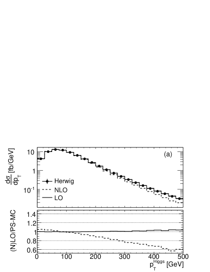
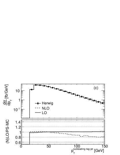
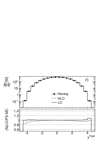
19.3.3 Reweighting of PS-MC

To partially account for the differences in the transverse momentum spectra, a simple reweighting method has been applied, where the Herwig events are weighted using the ratio to the NLO prediction in only one variable. This observable has been chosen to be the transverse momentum of the Higgs boson, since the differences are largest in this variable. The weights assigned to the Herwig events are chosen according to:

$$w=\frac{\frac{\mathrm{d}\sigma}{\mathrm{d}p_{T}^{\mathrm{H}}}(\mbox{NLO, MRST2004qed)}}{\frac{\mathrm{d}\sigma}{\mathrm{d}p_{T}^{\mathrm{H}}}(\mbox{Herwig, CTEQ6L1)}~{}~{}~{}}$$ (75)

The dashed Histogram in the lower part Figure 36 (a), which is the ratio between the NLO prediction from [9, 10] and the Herwig prediction after VBF cuts, was fitted with a 3rd order polynomial in $p_{T}^{H}$ to be used as a reweighting function for the Herwig events. In principle also the LO prediction could be taken from [9, 10], but the shape of the transverse momentum distribution of the Higgs boson is identical to the one from Herwig in this case.

Figure 37 shows the comparison of the differential distributions after the reweighting procedure. By construction, the Herwig prediction for the transverse momentum of the Higgs boson now fits exactly the one of the NLO prediction. But due to the kinematic correlations, also an improved description of the tag-jet transverse momenta and to a lesser extent the invariant dijet mass is obtained. The reweighted Herwig prediction is almost everywhere within 10% of the NLO prediction.

Figure 37: Differential distributions in after VBF cuts, including the reweighting procedure described in the text.

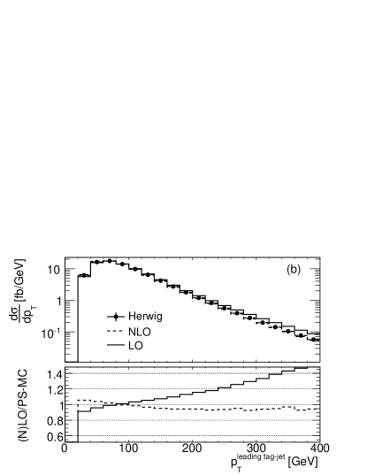
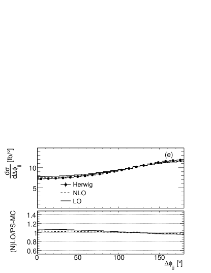
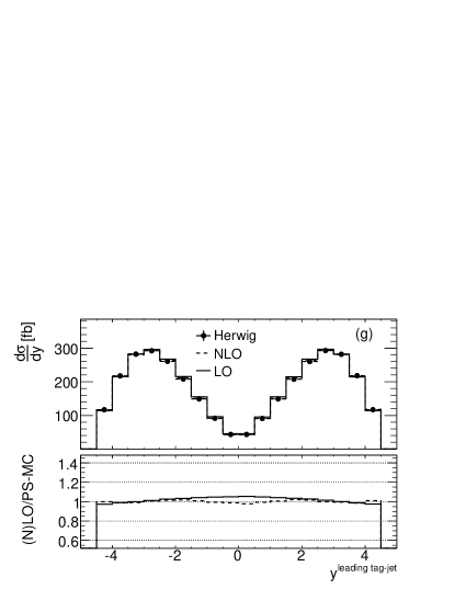
CONCLUSIONS

Acceptances and differential cross sections in the VBF process have been shown to agree between Herwig and the fixed order result from [9, 10] in LO. The differences between the NLO predictions and the LO result in differential cross sections can be partially taken into account by a reweighting of Herwig events using a weight that depends on the transverse momentum of the generated Higgs boson. In this way an improved description can be obtained, though it would be better to have a fully merged NLO PS-MC available. It should be noted that in the VBF process, the electroweak NLO corrections have comparable influence to the QCD corrections on the cross section and on the shape of differential distributions [9, 10], thus a NLO PS-MC would have to take the electroweak corrections also into account to give the best available description of the VBF process.

ACKNOWLEDGMENTS

M. Warsinsky acknowledges the support of the Initiative and Networking Fund of the Helmholtz Association, contract HA-101 (“Physics at the Terascale”). We would like to acknowledge the use of the computing resources provided by the Black Forest Grid Initiative.

20 A STUDY OF SMOOTH PHOTON ISOLATION: A NOVEL IMPLEMENTATION

20.1 Introduction

Many interesting physics signatures at the LHC involve the presence of single or multiple photons in the final state. These photons may either be produced directly, through the fragmentation of a quark or gluon, or else through the decay of a resonance - such as e.g. the Higgs boson. There are backgrounds to the measurement of photons, primarily through the fragmentation of jets to a leading $\pi^{o}$ or $\eta$, which carries most of the energy of the parent parton. Photon identification cuts, which examine the lateral and longitudinal development of the candidate photon shower, reject much of this background, with a typical efficiency for retaining real photons of the order of 80% for photon transverse energy larger than 40 GeV/c.

A large additional rejection factor can be obtained for this jet background by the imposition of an isolation cut on the candidate photon [425, 426]; in this isolation cut, a restriction is placed on the amount of additional energy that can be present in a cone about the photon direction. The tighter the isolation cut, the more background is removed from the photon candidate sample. The isolation cut also has the effect of removing most of the photon contribution arising from the fragmentation subprocesses, but should be structured so as to have a high efficiency for the retention of real, isolated photons. However, a tight isolation cut also has the undesireable effect of making the theoretical prediction unstable, due to the restriction of the available phase space for soft gluon emission. Typically, the isolation cut may be formulated as requiring either the transverse energy in the isolation cone to be less than a fixed fraction $\epsilon_{s}$ of the candidate photon transverse energy, $E_{T}^{\gamma}$, or requiring there to be less than a fixed amount of additional energy present. The latter requirement is typically used at the Tevatron and is motivated by the fact that most of the energy in the isolation cone results from the underlying event (and pileup), and so is independent of the photon energy .

Another way to define direct photons is the so-called “democratic approach" [427, 428], where photons and QCD partons are treated on the same footing when being clustered into jets, and direct photons are then defined by jets containing a photon which carries a large fraction (typically more than 70%) of the jet energy. A detailed study of this approach in the context of matrix element to parton shower merging has been performed recently in [270].

Another way of framing the isolation cut is due to Frixione [429]: a cone of fixed radius $R_{o}$ (which typically has been of the order of 0.4) is drawn around the photon axis. Then for all radii $R$ inside this cone, the amount of additional transverse energy, assumed to be due only to hadrons, inside the cone of radius R is required to satisfy the following condition

$$E_{T}^{had}<f(R)\;,$$ (76)

where the energy profile $f(R)$ is some continuous function of $R$, growing with $R$, and which falls to zero as $R\to 0$, typically like $R^{2n}$, for some $n>0$. The following form  for $f(R)$ has been used in this study:

$$f(R)=\epsilon_{s}\,E_{T}^{\gamma}\,\left[\frac{1-\cos R}{1-\cos R_{o}}\right]^{n}$$ (77)

In the formula above, $\epsilon_{s}$ and $n$ are positive numbers of order one. This isolation criterion allows soft gluons to be arbitrarily close to the photon direction, but requires the energy of partons emitted exactly collinear to the photon direction, to vanish. This ideally prevents the appearance of any final state collinear divergence in the partonic calculation; as a result, it prevents the involvement of any fragmentation contribution, insofar as the latter is treated as a collinear process. This greatly simplifies the theoretical calculation as the fragmentation part is quite cumbersome to calculate at NLO; this is considered as one of the major advantages of the Frixione isolation criterion . It is thus an important goal to be able to adapt both the theoretical and experimental analysis machinery coherently at the LHC to be able to utilize this type of isolation. This is the major motivation for this contribution.

20.2 Experimental Considerations

In order to adapt this criterion to the experimental situation, several considerations need to be taken into account. First, because of the finite size of the calorimeter cells used to measure the electromagnetic shower, the Frixione isolation cut must be applied only beyond a minimum distance of approximately 0.1 (in $\{\Delta\eta,\Delta\phi\}$ space). This allows a contribution from fragmentation in the innermost cone, and one has to check to which extent the fragmentation component is still suppressed. In addition, the transverse energy in the experimental isolation cone is deposited in discrete cells of finite size and this granularity must be taken into account in the theoretical calculation. The continuity criterion, initially proposed by Frixione, has thus been replaced by a discretized version consisting of a finite number of nested cones, together with the collection of corresponding maximal values for the transverse energy allowed inside each of these cones.

As mentioned previously, the dominant contribution to the energy deposited in the photon isolation cone is from the non-perturbative/semi-perturbative underlying event (UE), and, at higher luminosities, from additional minimum bias events occurring in the same beam crossing (pile-up) as foreseen in future LHC running. These sources result in energy deposits of a fairly uniform density over the area of the detector, which are uncorrelated with the collinear fragmentation processes that the Frixione isolation cut is designed to remove. Thus, it seems sensible to separate the analysis of the two sources of energy in the isolation cone. Hence, a determination of the transverse energy density may suffice for an estimation of the amount of underlying event/pileup transverse energy inside the isolation cone. One convenient way of determining this density was suggested by Cacciari, Salam and Soyez [431], in which the transverse energy density is calculated, on an event-by-event basis, by measuring the transverse energy in soft jets ($E_{T}<$ 20 GeV) using the $k_{T}$ algorithm with a D-parameter of 0.5. As the harder jets are not included in this density determination, the result is a measure of the amount of energy to be expected in the isolation cone from sources independent of the production of the photon. This energy can then be subtracted, as a flat background, from the amount of energy found in the isolation cone of the photon candidate, and the Frixione isolation criterion, modified for the experimental granularity, can then be run on the remaining energy distribution . Otherwise, to avoid the occasional possibility of arriving at a negative energy in the isolation cone, the UE/pileup energy determined by this technique can be added, again as a flat background, to the amount determined in the experimental analysis (along with the density allowed by the Frixione profile). Again, it should be emphasized that the UE/pileup transverse energy density determined in this manner is on an event-by-event basis, and thus independent of the luminosity conditions or any fluctuations that may have occurred in that particular crossing. Thus, to define an isolated photon for any theoretical calculation, only the Frixione isolation criterion needs to be applied, as the experimental/non-perturbative sources of transverse energy accumulation have already been accounted for.

20.3 Implementation

It is not clear a priori what the best parameters for the Frixione isolation criterion are. For this contribution to the Les Houches proceedings, we have examined the impact of varying $\epsilon_{s}$ and $n$ in the isolation cut applied to single photon production in the program Jetphox [432, 433, 434]. The parameter pairs examined for ($n,\epsilon_{s}$) are:

• (0.2,0.05)

• (0.2,1.0)

• (1.0,1.0)

• (1.0,0.5)

• (1.0,0.05).

We have calculated the direct and fragmentation components for single photon production, after the imposition of the discretized version of the Frixione isolation criterion for the above parameter pairs. We considered $pp$ collisions at 10 TeV LHC operation and the photon transverse energy range of 60 GeV/c to 240 GeV/c, using CTEQ66 PDFs and a common factorization/renormalization/fragmentation scale of $p_{T}^{\gamma}/2$ . The radius of the outermost isolation cone around the photon direction was set to $R_{o}=0.4$. To simulate the detector granularity, we considered an isolation criterion made up of 6 nested cones of respective radii:

• $R_{1}=0.1$

• $R_{2}=0.16$

• $R_{3}=0.22$

• $R_{4}=0.28$

• $R_{5}=0.34$

and $R_{6}=R_{o}=0.40$, with the corresponding maximal values of $E_{T}^{had}$ allowed in each of these cones given by

$$E_{T}^{j}=\epsilon_{s}\,p_{T\,\gamma}\,\left[\frac{1-\cos R_{j}}{1-\cos R_{o}}\right]^{n}$$ (78)

To carry out this study in practice, Jetphox has been modified in the following way. The discrete Frixione criterion has been parametrized in the form of a 2-dimensional array whose entries are the radii of each of the nested cones and the corresponding maximal transverse energy allowed inside each cone. The size of the array can be varied up to a maximum of 10 and is automatically handled by a Perl script. These maximal energies are calculated as the values taken at the radii $R_{j}$ by a profile function which can be specified at will by the user, and which was taken to be the function presented above. The criterion has been implemented at the level of the computation of the grid which is used for the partonic Monte Carlo event generation.

Figure 38: The Jetphox prediction for the photon $E_{T}$ distribution, for the parameter choice $n=0.2,\epsilon_{s}=0.05$ in the discrete form of the Frixione criterion. The triangles denote the direct component, the circles the fragmentation component.

Figure 39: The Jetphox prediction for the photon $E_{T}$ distribution, for the parameter choice $n=0.2,\epsilon_{s}=1.0$ in the discrete form of the Frixione criterion. The triangles denote the direct component, the circles the fragmentation component.

Jetphox acounts for the LO and NLO contributions for both the direct and fragmentation contributions. For the direct contribution, isolation is not relevant at LO, since, due to transverse momentum conservation, the recoiling parton lies opposite the photon in $\phi$. At NLO, at most one of the two final state partons can contribute to the energy in the isolation region (the other parton recoils in the away-side region). For the fragmentation contribution, the collinear remnants of fragmentation lie completely inside the innermost cone of radius $R_{1}=0.1$, and are accounted for in the calculation by the quantity $1-z$, where $z$ is defined as the fraction of the transverse energy of the fragmenting parton carried away collinearly by the photon. At NLO, the extra parton, labelled “5" in the figure below (the spectator w.r.t. the fragmentation process), can be emitted at any angle with respect to the parent parton. Hence, this 5th parton can fall either into the cone defined by $R<R_{1}$ , or into any of the annuli, $\{R_{1}<R<R_{2}\}$ to $\{R_{5}<R<R_{6}\}$, or outside the cone defined by the maximal radius $R_{6}$. The implementation of the criterion on the fragmentation contribution amounts to the following possibilities:

• if the extra parton “5" falls inside $R_{1}$, the criterion imposes

  $$\frac{1-z}{z}\,E_{T}^{\gamma}+p_{T}^{5}<E_{T}^{1}$$

• if the extra parton “5" falls in the annulus $\{R_{j}<R<R_{j+1}\},j=1,\ldots,5$, the criterion imposes

  $$\frac{1-z}{z}\,E_{T}^{\gamma} < E_{T}^{1}$$

  $$\frac{1-z}{z}\,E_{T}^{\gamma}+p_{T}^{5} < E_{T}^{j+1}$$

• if the extra parton “5" falls outside cone $R_{6}$, the criterion imposes

  $$\frac{1-z}{z}E_{T}^{\gamma}<E_{T}^{1}$$

Figure 40: The Jetphox prediction for the photon $E_{T}$ distribution, for the parameter choice $n=1,\epsilon_{s}=0.05$. Only the direct component is shown. The criterion was too stringent for the fragmentation component to be evaluated in this case.

Figure 41: The Jetphox prediction for the photon $E_{T}$ distribution, for the parameter choice $n=1,\epsilon_{s}=0.5$. The triangles denote the direct component, the circles the fragmentation component.

20.4 Results

The direct and fragmentation contributions are shown for the 5 parameter combinations in Figs. 39-42. As expected, changes in the isolation parameters have little impact on the direct contributions (which are affected only at NLO, by gluon radiation into the isolation cone), while most of the fragmentation contribution can be eliminated by isolation - except with the choice $(n=0.2,\epsilon_{s}=1)$ for which the photon isolation turns out to be very loose. In particular, in the innermost cone $R_{1}=0.1$, the photon can be accompanied by as much as 58% of the photon’s transverse energy, i.e. the accompanying hadronic $E_{T}$ in cone $R_{1}$ ranges from $\sim 35$ GeV for $E_{T}^{\gamma}=60$ GeV to $\sim 138$ GeV for $E_{T}^{\gamma}=240$ GeV. The parameter choice $(n=1,\epsilon_{s}=0.5)$ has a similar isolation effect in the innermost cone, i.e. on fragmentation, as the choice $(n=0.2,\epsilon_{s}=0.05)$ considered earler by [430], while the isolation energy profile of the former choice is much less stringent away from the photon’s direction than the latter.

Figure 42: The Jetphox prediction for the photon $E_{T}$ distribution, for the parameter choice $n=1,\epsilon_{s}=1$. The triangles denote the direct component, the circles the fragmentation component.

The comparison of the $\{$Direct+Fragmentation$\}$ Jetphox predictions with predictions using the continuous criterion as implemented in Frixione’s code for the above five parameters choices $(n,\epsilon_{s})$ are presented in Figs. 44-47. The two codes used different scale choices, $\mu=M=M_{F}=E_{T}^{\gamma}/2$ for Jetphox vs. $(E_{T}^{\gamma}+E_{T}^{jet})/4$ for Frixione respectively. Notice however that these two scales coincide at the Born level. There may be differences at NLO between the two, though hopefully not major ones. In addition, Jetphox used a frozen $\alpha_{em}$ whereas Frixione used a running $\alpha_{em}$ (at the above scale choice). Frixione’s choice for $\alpha_{em}$ systematically increases the prediction w.r.t. Jetphox, yet the net effect is likely dominated by the QCD scale dependence. The relative size of this effect is difficult to predict without performing a dedicated study. Nevertheless, the two calculations yield similar results, illustrating that the discrete form of the Frixione criterion retains the features of the continuous criterion, at least at the partonic level, and as long as the discrete criterion strongly suppresses the fragmentation component (i.e. all but $(n=0.2,\epsilon=1)$ in the parameter choices considered for illustration).

Figure 43: A comparison of the Jetphox $\{$Direct+Fragmentation$\}$ prediction for the photon $E_{T}$ distribution with the discrete criterion (open triangles) vs. Frixione with the continuous criterion (solid triangles), for the parameter choice $n=0.2,\epsilon_{s}=0.05$.

Figure 44: A comparison of the Jetphox $\{$ Direct + Fragmentation $\}$ prediction for the photon $E_{T}$ distribution with the discrete criterion (open triangles) vs. Frixione with the continuous criterion (solid triangles), for the parameter choice $n=0.2,\epsilon_{s}=1$.

Figure 45: A comparison of the Jetphox $\{$Direct+Fragmentation$\}$ prediction for the photon $E_{T}$ distribution with the discrete criterion (open triangles) vs. Frixione with the continuous criterion (solid triangles), for the parameter choice $n=1,\epsilon_{s}=0.05$.

Figure 46: A comparison of the Jetphox $\{$Direct+Fragmentation$\}$ prediction for the photon $E_{T}$ distribution with the discrete criterion (open triangles) vs. Frixione with the continuous criterion (solid triangles), for the parameter choice $n=1,\epsilon_{s}=0.5$.

Figure 47: A comparison of the Jetphox $\{$Direct+Fragmentation$\}$ prediction for the photon $E_{T}$ distribution with the discrete criterion (open triangles) vs. Frixione with the continuous criterion (solid triangles), for the parameter choice $n=1,\epsilon_{s}=1$.

20.5 Some Theoretical Issues

From a theoretical perspective, one might be concerned by the use of cone radii as small as 0.1-0.2, for which earlier studies [435] revealed potential problems. The earlier studies were carried out for the standard cone criterion, in the limit of a narrow cone, $R\ll 1$, while allowing a given $R$-independent energy deposit inside the cone. This lead to a collinear sensitivity in the form of a fairly large dependence on $\ln(1/R)$, which could make the prediction unreliable unless these logarithms were resummed. With the Frixione criterion, at least in its continuous version, the amount of energy inside the cone is a function of $R$, decreasing to 0 as $R$ decreases; this correlates the energy and angular variables in such a way as to prevent the appearance of collinear divergences, and thus should avoid the concomitant appearance of troublesome logs. Therefore, the potential problem discussed in  [435] regarding the appearance of large $\log R$ terms with the standard cone criterion, in the limit of narrow cone sizes ($R\ll 1$), is not expected in the present case, even though the discretization of the Frixione criterion mimics a standard cone criterion inside the innermost cone. In the discrete version studied here, the isolation in the innermost cone $R_{1}$ is effectively similar to the standard cone criterion with $(R_{1},E_{T\,1})$; however, unlike the situation with the standard criterion, the region outside cone $R_{1}$ is still constrained by the isolation condition $(R_{2},E_{T\,2})$ and so on. This prevents any similar worrisome $\ln(1/R_{j})$ dependence from developing.

Another topic of concern might be the behaviour of the fragmentation functions into a photon (FFP) when $z\to 1$, a regime which is enhanced by the requirement of a stringent isolation. It should be noted that the behaviour of the FFP in this regime is different from the corresponding one for hadrons. The FFP are controlled by the so-called anomalous component induced by the inhomogenous terms in the DGLAP evolution equations, arising from the point-like quark-photon coupling, and which are in principle fully calculable in perturbative QCD. The non-perturbative, hadronic part is comparatively negligible in this regime. Unfortunately, the NLO calculation of the FFP is plagued by large logarithms of the form $\ln^{k}(1-z)$, $k=1,2$ coming from both homogeneous and inhomogeneous DGLAP kernels, and which make the predictions quantitatively unreliable. On the other hand, one expects that for the cross sections involving an integral over the fragmentation variable $z$, this sensitivity to these integrable logarithms $\ln^{k}(1-z)$ is smeared over a narrow domain in $z$, thus yielding only a small contribution. We therefore expect that this issue is not too troublesome.

20.6 Summary and outlook

In this contribution, we have outlined an adaptation of the Frixione isolation criterion, modified to take into account the experimental environment in which the photon measurements will be conducted at the LHC. The resulting discrete version of the Frixione criterion provides isolated photon cross sections in good agreement with those obtained from the continuous version. Much of the energy in the isolation cone results not from the hard process, but from the soft underlying event from the collision producing the photon, or from additional interactions taking place in the same crossing. A method was outlined to separate the energy from these soft processes with energies resulting from fragmentation processes. With this separation, only the Frixione isolation criterion need be applied to any theoretical calculation.

In future studies, the techniques outlined here will be tested first against Monte Carlo data, and then against the early LHC data.

21 ON THE CORRELATION BETWEEN $\alpha_{s}\left(M_{Z}^{2}\right)$ AND PDFS WITHIN THE NNPDF APPROACH

21.1 Combined PDF and $\alpha_{s}$ uncertainties.

The impact of the combined $\alpha_{s}-$PDF uncertainties has been recently investigated by CTEQ [436] and MSTW [437]. In this contribution we discuss how the correlation between the strong coupling and PDFs affects PDF determination and uncertainties in physical observables within the NNPDF approach [438, 439, 440, 441, 442, 443, 444, 445, 446] to PDF determination. We show the impact that varying $\alpha_{s}$ has in the PDF determination, both for central values and for uncertainties. We then quantify the correlation between $\alpha_{s}$ and the gluon. Finally, we discuss different procedures to combine the uncertainties from PDFs and $\alpha_{s}$ in physical observables, and compare these procedures for the important case of Higgs production at the LHC.

21.2 NNPDF1.2 with varying $\alpha_{s}(M_{Z}^{2})$

The strong coupling is determined from a global average from a wide variety of different measurements. The current PDG value gives [447]

$$\alpha_{s}\left(M_{Z}^{2}\right)=0.1176\pm 0.002\ ,$$ (79)

where the error is to be interpreted as a 1-$\sigma$ uncertainty. Another recent world average [448] finds

$$\alpha_{s}\left(M_{Z}^{2}\right)=0.1184\pm 0.0007\ .$$ (80)

In the rest of this contribution we will take as reference value for $\alpha_{s}$ and its uncertainty the following range:

$$\alpha_{s}\left(M_{Z}^{2}\right)=0.119\pm 0.0012\ ,68\%\,{\rm C.L.}\qquad(\pm 0.0020\ ,89\%\,{\rm C.L.})\ ,$$ (81)

although the generalisation of the present study to any other value of the strong coupling and its uncertainty is straightforward.

The motivation of this contribution is to explore the impact of the uncertainties in $\alpha_{s}$, Eq. 81, in PDF determination and associated LHC observables. In order to do so, taking as reference the NNPDF1.2 parton determination [443], a set of fits with different values of alphas were produced, together with the associated PDF uncertainties in each case. In Fig. 48 we show the ratios of the central gluons obtained in these fits with varying $\alpha_{s}$ as compared to the reference NNPDF1.2 gluon with $\alpha_{s}=0.119$, together with the associated PDF uncertainty for this reference value. The sensitivity with respect the chosen value of $\alpha_{s}$ is non-negligible, although for $\alpha_{s}$ variations within the assumed uncertainty range Eq. 81 fall typically within the PDF uncertainty band.

It is easy to understand the qualitative behaviour of the gluon in Fig. 48. In a DIS-only fit like NNPDF1.2 [443], the gluon is essentially determined at small-$x$ through the scaling violations of HERA structure function data, and smaller values of $\alpha_{s}$ are compensated with harder small-$x$ gluons. At large-$x$ there are no experimental constrains on the gluon so it is essentially determined by the momentum sum rule, and thus its behaviour is anti-correlated to that of the small-$x$ region. In a global fit [437, 436] the behaviour is essentially the same modulo some constrains from the Tevatron inclusive jet data on the large-$x$ gluon.

Other PDFs are affected to a much lesser extent, as shown in Fig. 49. For example, the $\alpha_{s}$ dependence of the triplet or the total valence is clearly negligible when compared with the respective PDF uncertainties. The only possible exception is the singlet $\Sigma(x,Q^{2})$, determined with precision from HERA data and which is coupled to variations in the gluon through the momentum sum rule. However, even in this case variations are rather smaller than PDF uncertainties.

Figure 48: The ratios of the central gluons obtained in the fits with varying $\alpha_{s}$ as compared to the reference NNPDF1.2 gluon at the initial evolution scale $Q^{2}_{0}=2$ GeV². The comparison is shown both in a linear (left plot) and logarithmic (right plot) scales. The dashed band corresponds to the NNPDF1.2 gluon relative PDF uncertainty.

Figure 49: The ratios of the central PDFs obtained in the fits with varying $\alpha_{s}$ as compared to the reference NNPDF1.2 PDF, including PDF uncertainties, at the initial evolution scale $Q^{2}_{0}=2$ GeV². The PDFs shown here are from top to bottom and from left to right: the triplet $T_{3}$ in a linear scale, the total valence $V$ in a linear scale, the singlet $\Sigma$ in a log scale and the strange sea $s^{+}$ in a log scale.

Figure 50: Comparison of the absolute gluon PDF uncertainty obtained in the fits with varying $\alpha_{s}$ as compared to the reference NNPDF1.2 gluon. The comparison is shown both in a linear (left plot) and logarithmic (right plot) scales. Note that what is shown in the uncertainty on the PDF and not the PDF itself.

Figure 51: Comparison of PDF uncertainties obtained in the fits with varying $\alpha_{s}$ as compared to the reference NNPDF1.2 PDF. The absolute PDF uncertainties shown here are from top to bottom and from left to right: the triplet $T_{3}$ in a linear scale, the total valence $V$ in a linear scale, the singlet $\Sigma$ in a log scale and the strange sea $s^{+}$ in a log scale. Note that what is shown are the uncertainty on the PDFs and not the PDF themselves.

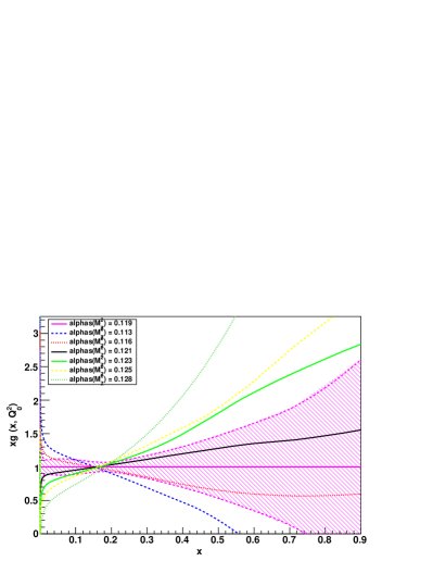
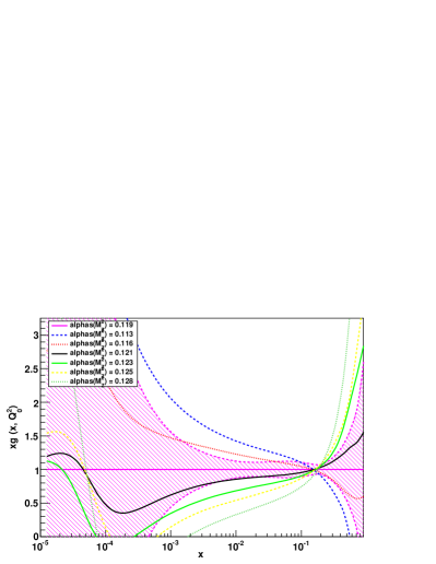
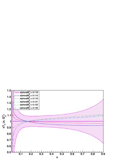
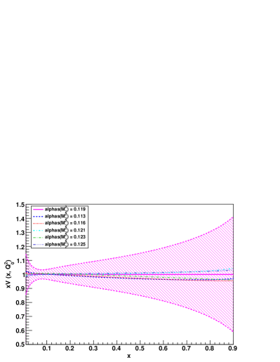
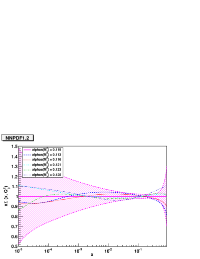
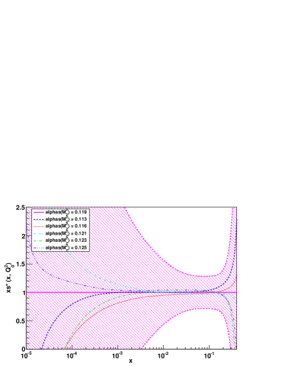
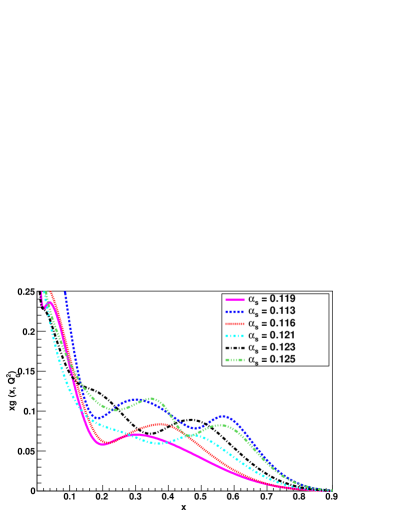
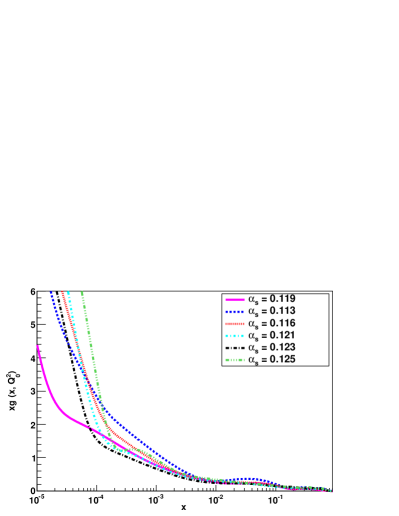
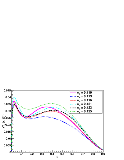
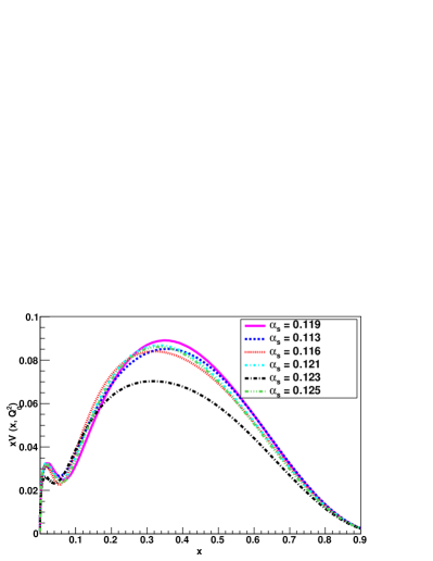
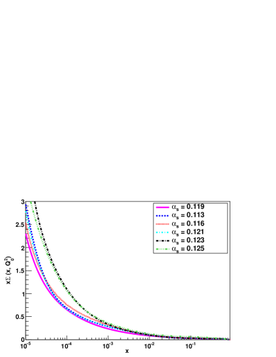
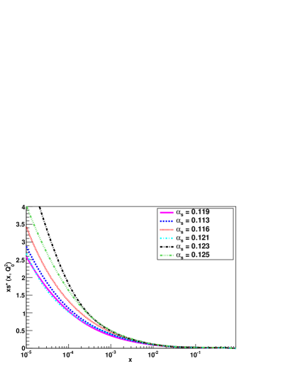
On top of the impact of variations in $\alpha_{s}$ in the PDF central values, also the PDF uncertainties are in principle modified by these variations. Within the Hessian approach (see for example Ref. [437]), which implies a simultaneous determination of $\alpha_{s}$ and the PDFs, $\alpha_{s}$ variations from the best fit value result in PDFs with reduced uncertainties by construction. This is however not necessarily the case if one does not assume a quadratic approximation of the $\chi^{2}$ as both PDF parameters and $\alpha_{s}$ are varied.

To assess quantitatively how PDF uncertainties are affected by $\alpha_{s}$ variations within the NNPDF approach, we show in Fig. 50 the absolute PDF uncertainties for the gluon for the different values of $\alpha_{s}$ obtained using the NNPDF1.2-like fits, and in Fig. 51 the same for other PDFs which are much less affected by $\alpha_{s}$ variations (see Figs. 48-49 respectively). In the case of the gluon, it seems that the reference value $\alpha_{s}\left(M_{Z}^{2}\right)=0.119$ tends to have the smaller PDF uncertainties, although as will be shown below essentially all values of $\alpha_{s}$ result in similar PDF uncertainties once fluctuations in the PDF uncertainties themselves are taken into account. For the other PDFs, Fig. 51, no such pattern can be identified and in any case the dependence of PDF uncertainties on $\alpha_{s}$ is much milder.

In order to determine whether such variations of the PDF uncertainty when $\alpha_{s}$ is varied in the fit are statistically significant, we need to compute the error on the PDF error itself. This is done automatically using the distance estimator, as for example done in Ref. [445]. Therefore we show in Fig. 52 the distances for central values and uncertainties for the gluons with different $\alpha_{s}$ as compared with the reference NNPDF1.2 gluon. We observe that for all the values of $\alpha_{s}$ the uncertainties in the gluon PDF are statistically equivalent, with the possible exception of the rather extreme value $\alpha_{s}\left(M_{Z}^{2}\right)=0.113$.

Figure 52: The distance between the NNPDF1.2 gluon and the NNPDF1.2-like gluons with different values of $\alpha_{s}\left(M_{Z}^{2}\right)$, both for central values (upper plots) and standard deviations (lower plots), as a function of $x$. All distances are computed from sets of $N_{\rm rep}=100$ replicas. A distance $d\sim 1$ corresponds to two fits which are statistically equivalent, while a distance $d\sim 10$ correspond to fits which differ by approximately 1-$\sigma$ [440, 445].

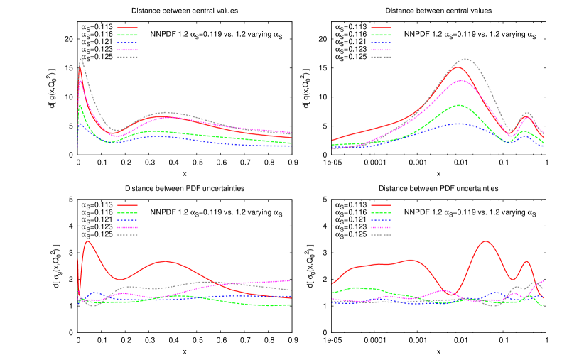
21.3 The correlation between $g(x,Q^{2})$ and $\alpha_{s}\left(M_{Z}^{2}\right)$

In order to make more quantitative the qualitative statements about the correlation between PDFs and $\alpha_{s}$, we can compute their correlation coefficient for any given values of $x$ and $Q^{2}$. The correlation between the strong coupling and the gluon (or in general any other PDF) is defined as the usual correlation between two probability distributions, namely

$$\rho\left[\alpha_{s}\left(M_{Z}^{2}\right),g\left(x,Q^{2}\right)\right]={{\left\langle\alpha_{s}\left(M_{Z}^{2}\right)g\left(x,Q^{2}\right)\right\rangle_{\mathrm{rep}}-\left\langle\alpha_{s}\left(M_{Z}^{2}\right)\right\rangle_{\mathrm{rep}}\left\langle g\left(x,Q^{2}\right)\right\rangle_{\mathrm{rep}}}\over{\sigma_{\alpha_{s}\left(M_{Z}^{2}\right)}\sigma_{g\left(x,Q^{2}\right)}}}\ .$$ (82)

Note that the computation of this correlation takes into account not only the central gluons of the fits with different $\alpha_{s}$ but also the corresponding uncertainties in each case.

Whereas the distribution of gluon distributions in Eq. (82) is given by the Monte Carlo sample, the distribution of $\alpha_{s}$ values is given by the procedure with which $\alpha_{s}$ is determined. Because we take $\alpha_{s}$ as determined from a global fit [447, 448] we assume its value to be gaussianly distributed, with the mean and standard deviation given by Eq. (81). We then fix the total number of PDF replicas to be used as

$$N_{\rm rep}=\sum_{j=1}^{N_{\alpha_{s}}}N^{\alpha_{s}^{(j)}}_{\rm rep}\ ,$$ (83)

where $N^{\alpha_{s}^{(j)}}_{\rm rep}$ is the number of PDF replicas, randomly selected from the fit obtained with the corresponding value of $\alpha_{s}$, $\alpha_{s}^{(j)}$, and $N_{\alpha_{s}}$ is the number of PDF determinations with different values of $\alpha_{s}$ which have been performed. The number of replicas for each different value of $\alpha_{s}$ to be used is thus, for a gaussian distribution,

$$N^{\alpha_{s}^{(j)}}_{\rm rep}\propto\exp\left(-{{\left(\alpha_{s}^{(j)}-\alpha_{s}^{(0)}\right)^{2}}\over{2\delta_{\alpha_{s}}^{2}}}\right)\ .$$ (84)

with $\alpha_{s}^{(0)}$ and $\delta_{\alpha_{s}}$ given in Eq. 81.

The average over Monte Carlo replicas of a general quantity which depends on both $\alpha_{s}$ and the PDFs, $\mathcal{F}\left({\rm PDF},\alpha_{s}\right)$, for example that of Eq. 82, has to be understood schematically as follows

$$\left\langle\mathcal{F}\right\rangle_{\mathrm{rep}}={{1}\over{N_{\mathrm{rep}}}}\sum_{j=1}^{N_{\alpha}}\sum_{k_{j}=1}^{N_{\rm rep}^{\alpha_{s}^{(j)}}}\mathcal{F}\left({\rm PDF}^{(k_{j},j)},\alpha_{s}^{(j)}\right)\ ,$$ (85)

where ${\rm PDF}^{(k_{j},j)}$ stands for the replica $k_{j}$ of the PDF fit obtained using $\alpha_{s}^{(j)}$ as the value of the strong coupling.

Our results for the correlation coefficient between the gluon and $\alpha_{s}(M_{Z}^{2})$ as a function of $x$, computed using Eq. 82 both at the input evolution scale $Q_{0}^{2}=2$ GeV² and at a typical LHC scale $Q^{2}=10^{4}$ GeV² are shown in Fig. 53. It is interesting to note how evolution decorrelates the gluon from the strong coupling. We also show in Fig. 53 the correlation coefficient for other PDFs: as expected for the triplet and valence PDFs it is essentially zero, that is, in NNPDF1.2 these PDFs show no sensitivity to $\alpha_{s}$, as was clear from Fig. 49.

The correlation coefficient Fig. 53 quantifies the qualitative observations of Figs. 48-49. This correlation coefficient could be used to correct the sum in quadrature of PDf and $\alpha_{s}$ uncertainties, though in practice it is simpler to just use the exact formula Eq. (85).

Figure 53: Left plot: The correlation coefficient, defined in Eq. 82, between the gluon and $\alpha_{s}(M_{Z}^{2})$ as a function of $x$, both at the input evolution scale $Q_{0}^{2}=2$ GeV² and at a typical LHC scale $Q^{2}=10^{4}$ GeV². Right plot: the analogous correlation coefficient for the singlet, triplet and total valence PDFs. The distribution of $\alpha_{s}\left(M_{Z}^{2}\right)$ has been assumed to be a gaussian with mean and standard deviation given by Eq. 81.

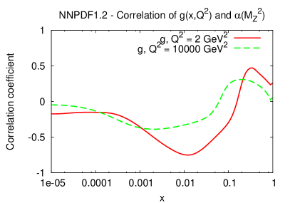
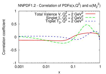
21.4 Strong coupling uncertainty in Higgs production

Let us consider a physical cross section which depends both on the PDFs and $\alpha_{s}$, and which will be denoted schematically by $\sigma\left({\rm PDF},\alpha_{s}\right)$. This cross-section has associated a PDF uncertainty $\delta\sigma_{\rm PDF}$, obtained from a fixed value $\alpha_{s}^{(0)}$. Different PDF groups provide different recipes to estimate this uncertainty. On the other hand, this cross section also has associated an uncertainty due to our limited knowledge of $\alpha_{s}$, $\delta\sigma_{\alpha_{s}}$. The simplest way of estimating this uncertainty is keeping the PDFs fixed to their central value, PDF⁽⁰⁾, which gives the following relative uncertainty

$${{\left(\delta\sigma\right)_{\alpha_{s}}^{\pm}}\over{\sigma}}={{\sigma\left({\rm PDF}^{(0)},\alpha_{s}^{(0)}\pm\delta_{\alpha_{s}}\right)}\over{\sigma\left({\rm PDF}^{(0)},\alpha_{s}^{(0)}\right)}}\ ,$$ (86)

where $\delta_{\alpha_{s}}$ is the assumed 68% confidence level range for $\alpha_{s}$, in our case given by Eq. 81.

Taking into account the presence of these two sources of uncertainties, PDFs and $\alpha_{s}$, there are at least three different recipees to determine the combined uncertainty in the cross-section $\sigma$, denoted by $\left(\delta\sigma\right)_{{\rm PDF}+\alpha_{s}}^{\pm}$. They can be ordered in order of formal accuracy

• The simplest approach consist in adding in quadrature the PDF and $\alpha_{s}$ uncertainties, where the latter is defined by Eq. 86. In this case the combined uncertainty will be given by

  $$\left(\delta\sigma\right)_{{\rm PDF}+\alpha_{s}}^{\pm}=\sqrt{\left[\left(\delta\sigma\right)_{\alpha_{s}}^{\pm}\right]^{2}+\left[\left(\delta\sigma\right)_{\rm PDF}^{\pm}\right]^{2}}\ .$$ (87)

  The main drawback of this approach is that it neglects the correlation between the PDFs and $\alpha_{s}$, which as we have seen in Sect. 21.2 is not negligible in principle.

• A more refined approach requires using PDFs obtained from different values of $\alpha_{s}$: this way it is possible to take properly into account the correlations between $\alpha_{s}$ and the PDFs. In this case, instead of using the approximation Eq. 86, the $\alpha_{s}$ uncertainty is evaluated with PDF sets obtained with the corresponding value of $\alpha_{s}$, namely,

  $${{\left(\delta\sigma\right)_{\alpha_{s}}^{\pm}}\over{\sigma}}={{\sigma\left({\rm PDF}^{(\pm)},\alpha_{s}^{(0)}\pm\delta_{\alpha_{s}}\right)}\over{\sigma\left({\rm PDF}^{(0)},\alpha_{s}^{(0)}\right)}}\ ,$$ (88)

  where PDF^(±) stands schematically for the PDFs obtained when $\alpha_{s}$ is varied within its 1-$\sigma$ range, $\alpha_{s}^{(0)}\pm\delta_{\alpha_{s}}$. Then the overall combined uncertainty will be given again by Eq. 87, but with Eq. 88 for the $\alpha_{s}$ uncertainties. This approach, while being a clear improvement with respect to the former, still misses some information on the correlations between $\alpha_{s}$ and the PDFs: it assumes that PDFs obtained with any value of $\alpha_{s}$ have the same uncertainties.

• The third and more accurate option is given by full correlated propagation of the PDF and $\alpha_{s}$ uncertainties into the cross section $\sigma$. The details of this approach will be different depending on the method used to determine the PDF uncertainties. Within the NNPDF approach (or more in general for any approach which uses the Monte Carlo method to estimate PDF uncertainties), this combined uncertainty is simply given by

  $$\left(\delta\sigma\right)_{{\rm PDF}+\alpha_{s}}^{\pm}=\sqrt{\left\langle\sigma^{2}\right\rangle_{\rm rep}-\left\langle\sigma\right\rangle^{2}_{\rm rep}}\ ,$$ (89)

  where the average over replicas (which include PDFs with different $\alpha_{s}$) is defined in Eq. 85 (note that here $\sigma$ denotes a cross–section, and $\delta\sigma$ the uncertainty on it).

As an illustration of the different procedures for the combined treatment of PDFs and $\alpha_{s}$ uncertainties within NNPDF, we have studied the specific case of Higgs production through gluon-gluon fusion, computing the cross-section uncertainties with the three different methods described above. As in the rest of the contribution, the range of $\alpha_{s}$ is taken to be that of Eq. 81, namely $\delta_{\alpha_{s}}=0.0012$ as a 68% confidence level.

As described below, in the simplest approach of sum in quadrature of the two uncertainties one needs to compute first the PDF uncertainty at fixed $\alpha_{s}$. In the particular case of the Higgs boson production cross section the PDF uncertainty can be estimated by computing the gluon-gluon luminosity,

$$\Phi\left(m_{H}^{2}\right)\equiv{{1}\over{S}}\int_{\tau}^{1}{{dx_{1}}\over{x_{1}}}g\left(x_{1},M_{H}^{2}\right)g\left(x_{2}=\tau/x_{1},m_{H}^{2}\right)\ ,$$ (90)

with $\tau=m_{H}^{2}/S$ and $\sqrt{S}$ the center of mass energy. At leading order, the Higgs cross section is simply proportional to Eq. 90.

This effective gluon-gluon luminosity as a function of the Higgs boson mass at the LHC with $\sqrt{S}=14$ and $\sqrt{S}=10$ TeV is shown in Fig. 54, where it is also compared to the same quantity from two other global PDF determinations: CTEQ6.6 [27] and MSTW08 [449]. We can see that at large $m_{H}$ the CTEQ6.6 and MSTW08 uncertainties are identical, while CTEQ6.6 is larger at small $m_{H}$. The NNPDF1.2 analysis results in the largest uncertainties, partially at least because the constrains from the hadronic data included in the other global analyses is not included.

Figure 54: The gluon-gluon luminosity, Eq. 90, computed at the LHC for $\sqrt{S}=14$ TeV (upper plots) and $\sqrt{S}=10$ TeV (lower plots) as a function of the Higgs boson mass for NNPDF1.2, as well as for MSTW08 and CTEQ6.6. In both cases we show both the 68% (left plots) and the 90% confidence levels (right plots). As expected, the impact of the different CMS energy in the PDF uncertainties is very reduced.

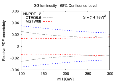
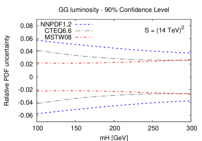
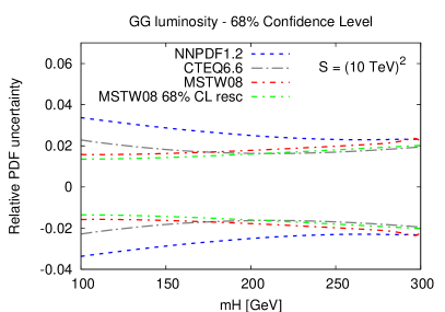
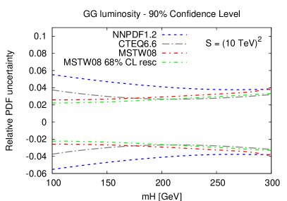
Now we turn to a discussion of the effect of the combination of PDF and $\alpha_{s}$ uncertainties in Higgs boson production. All numerical results discussed below have been obtained at NLO using the code of Refs. [450, 451]. In Fig. 55 we show the total cross section for Higgs boson production at the LHC as a function of $m_{H}$, computed with the NNPDF1.2 set, with the uncertainty band obtained by exact combination of the $\alpha_{s}$ and PDF uncertainties, both at 68% and 90% C.L.. The same figure also shows the relative uncertainties at 68% in the total cross section as computed from PDFs only.

In Fig. 56 we show a comparison of the 68% C.L. in the Higgs boson production cross section as a function of $m_{H}$ with the combined PDFs+$\alpha_{s}$ uncertainties, were exact error propagation is compared to the sum in quadrature of the two uncertainties. The sum in quadrature is done either by keeping the PDF fixed when $\alpha_{s}$ varied, or eles by taking the central best fit PDF set for each value of $\alpha_{s}$. Clearly, even the simplest sum in quadrature provides a very reasonable approximation to the exact result obtained with full error propagation. Therefore, one can conclude that, at least for the range of variation of $\alpha_{s}$ assumed, Eq. 81, and with the NNPDF1.2 parton fit, the naive sum in quadrature of the PDF and $\alpha_{s}$ uncertainties seems to be a good enough approximation to the full result for most practical purposes.

A more detailed study of the interplay between $\alpha_{s}$ and PDF uncertainties in Higgs production for various PDF sets will be presented elsewhere [452]

Figure 55: Left figure: The total cross section for Higgs boson production at the LHC as a function of $m_{H}$, computed with the NNPDF1.2 set. The red band is the combined PDF and $\alpha_{s}$ uncertainty obtained exact error propagation (see text for details) at 68% confidence level, while the green band is the corresponding 90% confidence level. Right figure: the relative uncertainties in the total cross section as computed from PDFs only (blue line) and combined PDFs and $\alpha_{s}$ uncertainties (red line) at 68% C.L., always with exact error propagation Eq. 89.

Figure 56: A comparison of the 68% C.L. uncertainties in the Higgs boson production cross section as a function of $m_{H}$ for NNPDF1.2 with the combined PDFs+$\alpha_{s}$ uncertainties, using the various methods for the combination discussed in the text. The red line corresponds to exact error propagation Eq. 89, the green line to the sum in quadrature of the two uncertainties in the case in which $\alpha_{s}$ and also the PDFs are varied simultaneously, and finally the blue line is the sum in quadrature where the PDFs are kept fixed to their value obtained in the fit with central $\alpha_{s}$, Eq. 87, see the text for a more detailed discussion. It is clear that the sum of uncertainties in quadrature even for fixed PDFs already provides a reasonable approximation to the full result.

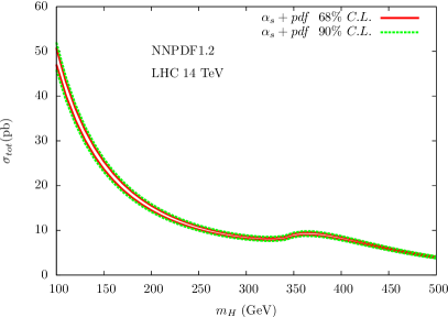
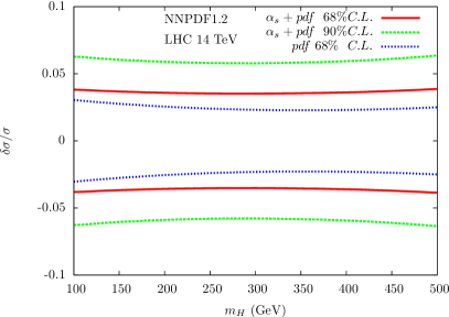
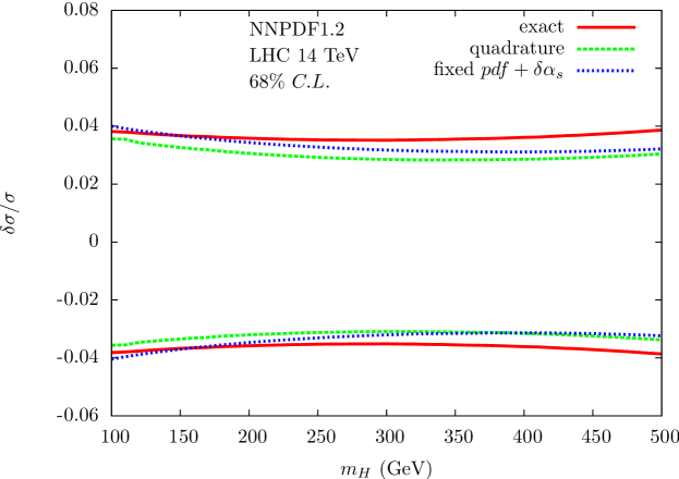
CONCLUSIONS

In this contribution we have studied the interplay between the strong coupling and PDF determination, and assessed the impact of the combined uncertainty one of the most sensitive processes to $\alpha_{s}$ variations, Higgs production through gluon-gluon fusion. The main result is that, at least within the NNPDF approach, even in a worst–case scenario like Higgs production at the LHC, the sum in quadrature of PDF and $\alpha_{s}$ uncertainties provides an excellent approximation to the full result obtained from exact error propagation.

22 THE LES HOUCHES BENCHMARKS FOR GM-VFN HEAVY QUARK SCHEMES IN DEEP-INELASTIC SCATTERING

22.1 Introduction

Interest in the inclusion of heavy flavour contributions to deep–inelastic electroproduction structure functions was recently revived by the discovery [453] that mass-suppressed terms in global parton fits can affect predictions for the total $W$ and $Z$ production at the LHC by almost 10 %. A technique for the inclusion of these mass-suppressed contributions to structure functions was developed long ago [454, 455], based upon a renormalization scheme with explicit heavy quark decoupling [456]. Several variants of this method (usually called ACOT) were subsequently proposed, such as S-ACOT [457] and ACOT-$\chi$ [458, 459]. However, the ACOT method was first used for an actual general-purpose global parton fit only recently, in Refs. [459, 453].

An alternative method (sometimes called TR) has also been advocated [462, 463], and used for all MRST parton fits until 2004 [464, 465, 466, 467]. Recently, however, the methods used by the CTEQ [453] and MRST/MSTW [468, 449] groups for their current parton fits, based respectively on the ACOT [454, 455] and TR^′ [469] procedures, have adopted at least in part a common framework: they have been compared recently in Refs. [470, 471], thereby elucidating differences and common aspects.

A somewhat different technique for the inclusion of heavy quark effects, the so-called FONLL method, was introduced in Ref. [472] in the context of hadroproduction of heavy quarks. The FONLL method only relies on standard QCD factorization and calculations with massive quarks in the decoupling scheme of Ref. [456] and with massless quarks in the $\overline{\text{{{MS}}}}$ scheme. The name FONLL is motivated by the fact that the method was originally used to combine a fixed (second) order calculation with a next-to-leading log one; however, the method is entirely general, and it can be used to combine consistently a fixed order with a resummed calculations to any order of either. The application of the FONLL scheme to deep–inelastic structure functions was recently presented in Ref. [473]. Thanks to its simplicity, the FONLL method provides a framework for understanding differences between other existing approaches, and for a study of the effect of different choices in the inclusion of subleading terms.

It is the aim of this contribution to update previous comparisons of GM-VFN schemes in DIS [470, 471] from a rather more quantitative point of view. Therefore, after unique settings have been adopted for all parties involved, the heavy quark structure functions $F_{2c}$ and $F_{Lc}$, as implemented in the various available approaches, have been computed and compared in detail. This comparison is of extreme importance in order to understand how parton distribution sets obtained from different schemes might differ, and what are the associated implications for LHC observables.

The outline of this contribution is the following. First of all, we present the benchmark settings for the computation of charm structure functions. Then we present the results for the comparison between the different schemes considered: ACOT, TR^′ and FONLL, and discuss their similarities and differences. Finally we summarize and provide benchmark tables which should be used for other GM-VFN schemes not considered here, either existing, updated or completely new.

22.2 Benchmark settings

Let us discuss now the settings for the benchmark comparisons between different GM-VFN schemes. These settings have been designed to isolate only the potential similarities and differences between GM-VFN schemes, while other choices that are generally varied between PDF fitting groups (like, for example, the value of $\alpha_{s}$) are shared among all the parties.

The goal of the benchmark comparison is to produce and compare results for the charm structure functions $F_{2c}$ and $F_{Lc}$ (for which we adopt the notation of Ref. [473]), computed at different values of $x$ and $Q^{2}$ from a variety of GM-VFN schemes.

These settings which we adopt for the benchmark comparison are the following:

• As input PDF set, the Les Houches initial conditions [474, 475] are used, with the initial scale for the PDF and $\alpha_{s}$ evolution taken to be $Q_{0}^{2}=2$ GeV². The initial $\alpha_{s}(Q_{0}^{2})=0.35$.

• The charm mass is taken to be $m_{c}=Q_{0}=\sqrt{2}$ GeV at NLO. At NNLO, both PDFs and $\alpha_{s}$ are discontinuous at $Q^{2}=m_{c}^{2}$ in a VFN scheme. We take the input PDFs and $\alpha_{s}$ at $Q_{0}=\sqrt{2}$ GeV to correspond to $N_{f}=3$, i.e. the charm mass is taken to be $m_{c}=(\sqrt{2}+\epsilon)$ GeV, for infinitesimal $\epsilon$, so that the appropriate NNLO discontinuities present at $Q^{2}=m_{c}^{2}$ are added to the input values before evolving to higher $Q^{2}$.

• The PDFs have been evolved with HOPPET [476], an $x-$space PDF evolution code, and interpolated in grids for easier interfacing with the various programs. Any other evolution code whose accuracy has been benchmarked with HOPPET like PEGASUS [477] would be equally valid.

• The charm quark is the only heavy quark present in the theory; the bottom and top quark masses are taken to infinity. This way complications arising from the presence of multiple heavy quarks are not considered.

• The $Q^{2}$ range of these benchmarks is from $Q^{2}=4$ GeV² (near the heavy quark threshold) to $Q^{2}=100$ GeV² (which is close to the asymptotic limit for practical purposes). Appropriate intermediate values are $Q^{2}=10$ and 24 GeV².

• The strong coupling constant $\alpha_{s}(Q^{2})$ is computed by means of exact numerical integration of the evolution equations (as usually done in $x-$space codes like HOPPET) instead of one of the various possible expanded solutions. The initial $\alpha_{s}(Q_{0}^{2})=0.35$ at both NLO and NNLO. Again, we take $m_{c}=(\sqrt{2}+\epsilon)$ GeV at NNLO, so that the input scale $Q_{0}=\sqrt{2}$ GeV corresponds to $N_{f}=3$. With this choice, the values of $\alpha_{s}$ to be used in the benchmark computations will be given by:

  $$\alpha_{s}\left(Q^{2}=4\,{\rm GeV}^{2}\right) = 0.295\,\,(0.295)\ ,$$

  $$\alpha_{s}\left(Q^{2}=10\,{\rm GeV}^{2}\right) = 0.245\,\,(0.244)\ ,$$

  $$\alpha_{s}\left(Q^{2}=24\,{\rm GeV}^{2}\right) = 0.212\,\,(0.211)\ ,$$ (91)

  $$\alpha_{s}\left(Q^{2}=100\,{\rm GeV}^{2}\right) = 0.174\,\,(0.173)\ ,$$

  at NLO (and NNLO) respectively for the values of $Q^{2}$ used for the benchmarks.

• As discussed in Refs. [478, 473], from $\mathcal{O}\left(\alpha_{s}^{2}\right)$ there is an ambiguity in the definition of the heavy quark structure functions from terms in which a light quark couples to the virtual photon. For these benchmarks, $F_{2c}$ and $F_{Lc}$, the heavy quark structure functions, are always defined as the sum of the contributions in which a charm quark is struck by the virtual photon, as opposed to the widely used experimental definition, which is the sum of all the contributions in which a charm quark is present in the final state. This definition avoids the presence of infrared unsafe terms from the non-cancellation of mass singularities.

22.3 General–Mass heavy quark schemes

As discussed in the introduction, the aim of the benchmark comparison is to identify similarities and differences between the GM-VFN schemes which are, have been or will be used in global PDF determinations. Without the purpose of being comprehensive, we present now a brief introduction of the three approaches which are compared in this contribution: ACOT (used in the CTEQ family of PDF fits), TR/TR^′ (used in the MRST/MSTW family) and FONLL (currently being implemented in the NNPDF family). The interested reader can find all relevant technical details in the quoted bibliography.

For simplicity, all the discussion in this section assumes a single heavy quark with mass $m_{c}$, since the case of the charm quark is the one with the most phenomenological importance.

22.3.1 ACOT

The ACOT renormalization scheme [479, 455] provides a mechanism to incorporate the heavy quark mass into the theoretical calculation of heavy quark production both kinematically and dynamically. This is built upon the Collins-Wilczek-Zee (CWZ)[456] renormalization procedure which provides a formal foundation for the ACOT scheme which is valid to all orders. The CWZ renormalization ensures there are no large logarithms of the form $\ln(m_{c}/Q)$, and yields manifest decoupling of the heavy quarks in the $m_{c}\gg Q$ limit. In 1998 Collins [454] extended the factorization theorem to address the case of heavy quarks; this work ensures we can compute heavy quark processes to all orders. Thus, the ACOT scheme yields the complete quark mass dependence from the low to high energy regime; for $m_{c}\gg Q$ it ensures manifest decoupling, and in the limit $m_{c}\ll Q$ it reduces precisely to the $\overline{{\rm MS}}$ scheme without any finite renormalization terms.

As a result of the Collins [454] proof, it was observed that the heavy quark mass could be set to zero in certain pieces of the hard scattering terms without any loss of accuracy. This modification of the ACOT scheme goes by the name Simplified-ACOT (S-ACOT) and can be summarized as follows.

S-ACOT:

For hard-scattering processes with incoming heavy quarks or with internal on-shell cuts on a heavy quark line, the heavy quark mass can be set to zero ($m_{c}=0$) for these pieces. [457]

If we consider the case of NLO DIS heavy quark production, this means we can set $m_{c}=0$ for both the LO terms ($QV\to Q$) and the NLO quark-initiated terms (both the real $QV\to Qg$ and the virtual $QV\to Q$) as this involves an incoming heavy quark. We can also set $m_{c}=0$ for the subtraction terms as this has an on-shell cut on an internal heavy quark line; this includes both the gluon-initiated process: $(g\to Q\bar{Q})\otimes(QV\to Q)$ as well as the quark initiated process: $(Q\to gQ)\otimes(QV\to Q)$. Hence, the only contribution which requires calculation with $m_{c}$ retained is the NLO $gV\to Q\bar{Q}$ process.

In the conventional implementation of the heavy quark PDFs, we must “rescale” the Bjorken $x$ variable as we have a massive parton in the final state. The original rescaling procedure is to make the substitution $x\to x(1+m_{c}^{2}/Q^{2})$ which provides a kinematic penalty for producing the heavy charm quark in the final state [480]. As the charm is pair-produced by the $g\to c\bar{c}$ process, there are actually two charm quarks in the final state—one which is observed in the semi-leptonic decay, and one which goes down the beam pipe with the proton remnants. Thus, the appropriate rescaling is not $x\to x(1+m_{c}^{2}/Q^{2})$ but instead $x\to\chi=x(1+(2m_{c})^{2}/Q^{2})$; this rescaling is implemented in the ACOT–$\chi$ scheme, for example [481, 482, 458]. The factor $(1+(2m_{c})^{2}/Q^{2})$ represents a kinematic suppression factor which will suppress the charm process relative to the lighter quarks.

22.3.2 Thorne-Roberts (TR/TR^′)

The TR scheme was introduced in Refs. [462, 463] as an alternative to ACOT [455] with more emphasis on correct threshold behaviour. Like the ACOT scheme it is based on there being two different regions separated by a transition point, by default $Q^{2}=m_{c}^{2}$. Below this point a heavy quark is not an active parton but is generated in the final state using fixed-flavour (FF) coefficient functions, while above this point the heavy quark becomes a new parton, evolving according to the massless evolution equations, and structure functions are obtained using variable-flavour (VF) coefficient functions which must tend to the correct massless $\overline{\rm MS}$-scheme limits as $Q^{2}/m_{c}^{2}\to\infty$, up to possibly higher-order corrections. The relationships between the partons below and above the transition point are obtained from the transition matrix elements $A_{ij}(z,m_{c}^{2}/\mu^{2})$ calculated to ${\cal O}(\alpha_{s}^{2})$ in Ref. [483], which fortuitously result in continuity up to NLO in the $\overline{\rm MS}$-scheme.

The definition of the scheme is therefore equivalent to the definition of the VF coefficient functions. These are found by imposing the exact all-orders equivalence of the structure functions described using the FF scheme and the VF scheme. This provides a relationship between the coefficient functions in the two cases via the equation

$$C^{\rm FF}_{j}=\sum_{i}C^{\rm VF}_{i}\otimes A_{ij},$$ (92)

where the sum is over all the different partons in the VF description. This equivalence effectively defines the subtraction of the large logarithms in $Q^{2}/m_{c}^{2}$ in the FF coefficient functions in the correct manner. It was applied to obtain relationships in the asymptotic limit in Refs. [484, 483], and used to define the BMSN scheme in Ref. [483], but in Refs. [462, 463] it was used to define the VF coefficient functions for all $Q^{2}>m_{c}^{2}$. The definition is not unique because there are more coefficient functions on the right than on the left of Eq. 92, because of the extra heavy quark coefficient function on the right-hand side. As $Q^{2}/m_{c}^{2}\to\infty$ all VF coefficient functions must tend to the massless $\overline{\rm MS}$-scheme limit, but at finite $Q^{2}$ there is a freedom in the heavy quark coefficient functions, beginning with the zeroth-order ($C^{{\rm VF},(0)}_{c}$). Via Eq. 92 this affects other coefficient functions, e.g.

$$C^{{\rm FF},(1)}_{2c,g}\equiv C^{{\rm VF},(0)}_{2c,c}\otimes A^{(1)}_{cg}+C^{{\rm VF},(1)}_{2c,g},$$ (93)

so the choice of $C^{{\rm VF},(0)}_{2c,c}$ also defines $C^{{\rm VF},(1)}_{2c,g}$.

In the TR scheme [462, 463] the approach is to make a choice where all coefficient functions obey the correct threshold $W^{2}\geq 4m_{c}^{2}$ for heavy quark pair production. This was first imposed by defining the heavy quark coefficient functions such that the evolution $\partial F_{2c}/\partial\ln Q^{2}$ is continuous order-by-order at the transition point (possible only in the gluon sector beyond LO). This was used in subsequent MRST global analyses up to MRST 2004 [467]. However, it results in expressions which become increasingly complicated at higher order.

In Ref. [458] the correct threshold behaviour was achieved by using the simple approach of replacing the limit of $x$ for convolution integrals with $\chi=x(1+4m_{c}^{2}/Q^{2})$. In the case that the heavy flavour coefficient functions are just the massless ones with this restriction one obtains the S-ACOT($\chi$) approach. A very similar definition for heavy flavour coefficients was adopted in Ref. [469], resulting in the TR^′ scheme, and extended explicitly to NNLO. This TR^′ scheme was first used in the MRST 2006 analysis [468], and has been used in all subsequent MSTW analyses (see Sect. 4 of Ref. [449]).

There is one other aspect to the TR/TR^′ scheme definition. For $F_{2c}$ the relative order of the FF and VF coefficient functions is different, i.e. the former begin at first order in $\alpha_{s}$ and the latter at zeroth order. One cannot simply adopt the correct ordering above and below the transition point since then there would be a discontinuity in the structure function at $Q^{2}=m_{c}^{2}$, and because higher order effects are large at small $x$ and $Q^{2}$, this would be phenomenologically significant. The procedure adopted is to freeze the highest order part of the FF expression (i.e. ${\cal O}(\alpha_{s})$ at LO, ${\cal O}(\alpha_{s}^{2})$ at NLO, etc.), and keep this in the expression above $Q^{2}=m_{c}^{2}$. Hence, there is an additional, strictly higher order contribution in this region which becomes less important as $Q^{2}$ increases, but never vanishes even at asymptotic $Q^{2}$. At NNLO this requires producing a model for the ${\cal O}(\alpha_{s}^{3})$ FF coefficient functions from the known small-$x$ and threshold limits [469].

22.3.3 FONLL

The FONLL scheme was first introduced in the context of heavy flavour hadroproduction in Ref. [472]. It is based upon the idea of looking at both the massless and massive scheme calculations as power expansions in the strong coupling constant, and replacing the coefficient of the expansion in the former with their exact massive counterpart in the latter, when available. A detailed description of the FONLL method for DIS has been given in Ref. [473].

In Ref. [473] three FONLL scheme implementations have been proposed: scheme A, where one uses the NLO massless scheme calculation, matched with the LO (i.e. ${\cal O}(\alpha_{s})$) massive scheme calculation; scheme B, where one uses the NLO massless scheme calculation, matched with the NLO (i.e. ${\cal O}(\alpha_{s}^{2})$) massive scheme calculation; and scheme C, where one uses the NNLO massless scheme calculation, matched with the NLO massive scheme calculation.

Among the three schemes, scheme B has a peculiarity in the way the matching is performed. In fact, the massless scheme calculation of $F_{2c}$ at NLO expanded up to order $\alpha_{s}^{2}$ has the form $\alpha_{s}+\alpha_{s}L+\alpha_{s}^{2}L^{2}+\alpha_{s}^{2}L$, with $L\equiv\ln Q^{2}/m_{c}^{2}$, i.e. terms of order $\alpha_{s}^{2}$ with no logarithms are missing. On the other hand, in the massive coefficients the full $\alpha_{s}^{2}$ term is present. In this case, what one subtracts from the massless result is not simply the massless limit of the massive result, but only a part of it, not including the constant (i.e. without factors of $L$) term of order $\alpha_{s}^{2}$. As a consequence, these order $\alpha_{s}^{2}$ terms are not subtracted from the massive coefficient functions and persist as strictly higher-order contributions at high $Q^{2}$.

It is easily seen that the scheme A in the FONLL calculation should be equivalent to the S-ACOT scheme. If a $\chi$-scaling prescription is applied to all terms computed in the massless approximation, scheme A should become equivalent to the S-ACOT-$\chi$ prescription. Scheme B does not correspond to any S-ACOT calculation. It is more reminiscent of the TR method, where at the NLO level the full NLO massive result is also used. However, as we will shown below, this is only true at $Q^{2}=m_{c}^{2}$, since in the TR method the higher order term in the massive calculation is frozen at threshold. We conjecture that scheme C should again be equivalent to a NNLO generalization of the S-ACOT scheme.

Finally, let us mention that the FONLL GM-VFN scheme is currently being implemented in the NNPDF family of fits [440, 441, 442, 443], which up to now have been obtained in the zero–mass scheme for heavy quarks. Both schemes (A and B) will be implemented in the NLO NNPDF fits, and the theoretical uncertainties arising from the inherent ambiguities in the matching procedure will be thoroughly studied.

22.4 Results and discussion

We turn now to discuss the results of the quantitative comparison between the GM-VFN approaches described above, using the benchmark settings introduced in Sect. 22.2 First of all, we will discuss the comparison between FONLL and S-ACOT: we will show that FONLL-A is identical to S-ACOT, with and without threshold prescriptions. Having settled this point, we will turn to studying the similarities and differences between the FONLL and TR^′ schemes, this time both at NLO and at NNLO. This last set of comparisons are also equivalent to comparing S-ACOT with TR^′.

First of all, however, let us mention that there exist at least two different implementations of the $\chi$-scaling threshold prescription used in the literature. The first form of $\chi-$scaling is given by

$$F^{({\chi})}_{2c}(x,Q^{2})\equiv x\int_{\chi(x,Q^{2})}^{1}{{dy}\over{y}}C\left({{\chi(x,Q^{2})}\over{y}},\alpha_{s}(Q^{2})\right)f(y,Q^{2})\ ,$$ (94)

which is adopted by default in FONLL and also in the CTEQ6.5/6.6 [453, 27] PDF fits. On the other hand, one can use an alternative form of $\chi-$scaling,

$$F^{({\chi,{\rm v2}})}_{2c}(x,Q^{2})\equiv\chi\int_{\chi(x,Q^{2})}^{1}{{dy}\over{y}}C\left({{\chi(x,Q^{2})}\over{y}},\alpha_{s}(Q^{2})\right)f(y,Q^{2})\ ,$$ (95)

which is used, for example, in the TR^′ definition, and is equivalent to the unambiguous result in charged-current charm production from strange quarks where $F_{2c}(x,Q^{2})=\xi s(\xi,Q^{2})$ at leading order with $\xi=x(1+m_{c}^{2}/Q^{2})$. For neutral-current scattering, in both cases, Eq. 94 and Eq. 95, the scaling variable is given by

$$\quad\chi(x,Q^{2})=x\left(1+{{4m^{2}_{c}}\over{Q^{2}}}\right).$$ (96)

It is clear that the two forms of the prescription, Eqs. 94 and 95, differ only by a mass suppressed term $\left(1+4m_{c}^{2}/Q^{2}\right)$, and therefore are formally equivalent, although can be numerically quite different depending on the matching scheme adopted. These differences represent an inherent ambiguity of the matching procedure. Let us finally note that even the choice of scaling variable Eq. 96 is arbitrary: indeed, in Ref. [485] a one-parameter family of such scaling variables was explored.

22.4.1 Comparison of FONLL and S-ACOT

Let us begin with the comparison between FONLL and S-ACOT for $F_{2c}(x,Q^{2})$. Since the ACOT scheme has only been implemented at NLO, we restrict the comparison to the FONLL-A scheme. The ACOT scheme is extensible to higher orders, but the NNLO is only in progress. First of all, the Simplified ACOT (S-ACOT) scheme, introduced in Sect. 22.3.1, is compared to FONLL scheme A (see Sect. 22.3.3) in Figs. 57 and 58 at the benchmark kinematical points. The only difference between Figs. 57 and 58 is the choice of $\chi-$scaling threshold prescription adopted in FONLL scheme-A: while in Fig. 57 the default FONLL choice Eq. 94 is adopted, in Fig. 58 the alternative form Eq. 95 is used instead. In both figures, the S-ACOT-$\chi$ (v2) curve is computed with the definition of Eq. 95.

From this comparison it is clear that, without any threshold prescriptions, $F_{2c}$ in S-ACOT is identical to FONLL-A, and moreover that S-ACOT-$\chi$ is identical to FONLL-A-$\chi$, once $\chi$-scaling is understood as in Eq. 95. The comparison between the FONLL-A-$\chi$ curves in Figs. 57 and 58 shows that in this scheme (as in S-ACOT) the impact of the choice of arbitrary threshold prescription at low and moderate $Q^{2}$ can be as large as the resummation itself. Again, let us emphasize that when the same threshold prescriptions are applied the S-ACOT and FONLL-A schemes give always the same results (within minor numerical differences like integration errors).

It is also interesting to compare the S-ACOT scheme with the full ACOT scheme [479, 455]. In Fig. 59 we show the results of this comparison. Since ACOT and S-ACOT differ only by mass-suppressed terms, their difference turns out to be as expected very small, and essentially vanishes already for $Q^{2}\sim 10$ GeV². Therefore, for $Q^{2}\mathrel{\hbox to0.0pt{\lower 4.0pt\hbox{\hskip 1.0pt$\sim$}\hss}\raise 1.0pt\hbox{$>$}}10$ GeV² the full ACOT calculation is identical to the FONLL-A scheme.

We would like to note that the full ACOT scheme was used only in the CTEQ HQ series (HQ4 [460], HQ5 [461] and HQ6 [459]), while instead the zero-mass approximation was adopted in the general purpose CTEQ4M [486], CTEQ5M [461] and CTEQ6M [171] PDF sets. When CTEQ adopted a GM-VFN as default in their fits (starting from CTEQ6.5 [453]), the GM-VFN scheme adopted was instead S-ACOT-$\chi$. As it is clear from the comparison between Figs. 57 and 58, the main difference is the choice of threshold prescription, formally subleading but which can be numerically as large as the whole effect of the resummation itself, and which could have important phenomenological implications.

Finally, let us compare the results for the charm component of the longitudinal structure function $F_{Lc}(x,Q^{2})$. The results of these comparisons are shown in Fig. 60 for the case of FONLL-A and S-ACOT without threshold prescriptions. We can see that both schemes coincide also in this case, as was the case for $F_{2c}$.

In summary, we have shown that when threshold prescriptions are switched off, FONLL-A and S-ACOT are completely identical, both for $F_{2c}$ and $F_{Lc}$. This is also the case when $\chi-$scaling is adopted as a threshold prescription, but only when the same of the two possible implementations Eqs. 94-95 is consistently used in both cases. Finally, we have shown that the full ACOT result is numerically very close to S-ACOT (and thus FONLL-A), being numerically equivalent for $Q^{2}\geq 10$ GeV².

Figure 57: The $F_{2c}$ structure function for $Q^{2}=4$, 10, 24 and 100 GeV² in the FONLL scheme A (plain and with $\chi-$scaling) compared to the Simplified ACOT (S-ACOT) and S-ACOT-$\chi$ schemes. Note that the FONLL-A-$\chi$ scheme implements the threshold prescription as in Eq. 94, and the S-ACOT-$\chi$ (v2) curve is computed with the definition of Eq. 95.

Figure 58: Same as Fig. 57, but now the FONLL-A-$\chi$ scheme implements the threshold prescription as in Eq. 95.

Figure 59: The $F_{2c}$ structure function for $Q^{2}=4$, 10, 24 and 100 GeV² in the FONLL scheme A (plain) compared to the Simplified ACOT (S-ACOT) and full ACOT schemes.

Figure 60: The $F_{Lc}$ structure function for $Q^{2}=4$, 10, 24 and 100 GeV² in the FONLL scheme A (plain) and Simplified ACOT (S-ACOT) schemes.

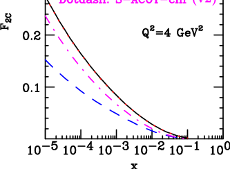
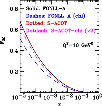
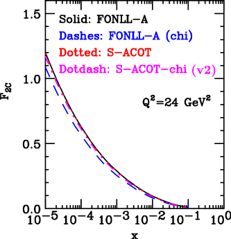
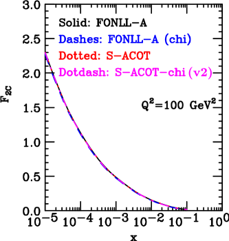
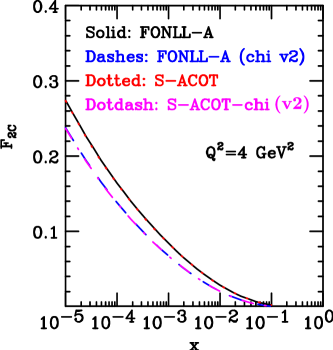
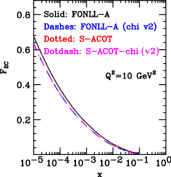
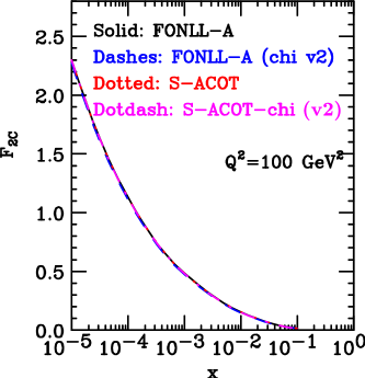
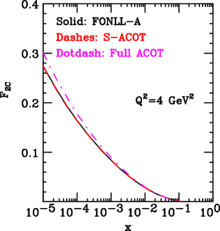
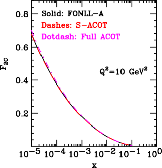
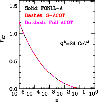
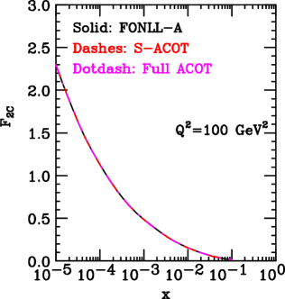
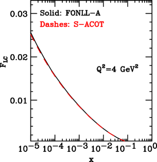
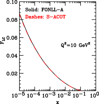
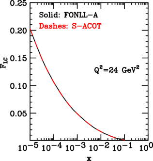
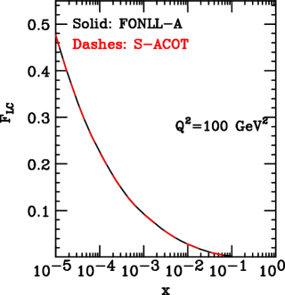
22.4.2 Comparison of FONLL and TR^′

Let us now discuss the results of the comparison between FONLL and the TR^′ scheme which has been used in the MSTW 2008 NLO and NNLO parton fits [449], as is introduced in Sect. 22.3.2. As shown in the previous section, all the results of this comparison apply both to FONLL-A and S-ACOT, which are numerically identical.

First of all, we show in Figs. 62-63 a comparison of the FONLL results with the results from the TR^′ NLO and NNLO GM-VFN schemes for the $F_{2c}$ structure function at the benchmark kinematical points. Unlike the ACOT case, since TR^′ has been formulated also up to NNLO, now we compare both the FONLL NLO schemes (A and B) with TR^′ NLO and separately the FONLL NNLO scheme (denoted by C) with TR^′ NNLO. From Figs. 62-63 no obvious similarities can be identified between the two families of schemes, neither at NLO nor at NNLO, apart from the obvious remark that differences between schemes decrease when $Q^{2}$ is increased.

In order to render the comparison more meaningful, the threshold prescriptions are switched off in both cases in Figs. 64-65. Having done this, it is clear that FONLL-A is rather close to TR^′ NLO, while in turn FONLL-C is rather close to TR^′ NNLO. Indeed, it can be shown that the two schemes differ only by a constant ($Q^{2}$-independent) term which is formally higher order and that is included in the TR^′ schemes in order to ensure continuity of physical observables at the heavy quark threshold. This is verified explicitly in Fig. 61.

Figure 61: Left plot: Absolute difference between $F_{2c}$ in the TR^′ NLO and FONLL-A schemes, in both cases without any threshold damping factor. Right plot: same between the TR^′ NNLO and FONLL C-schemes.

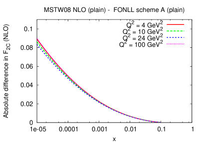
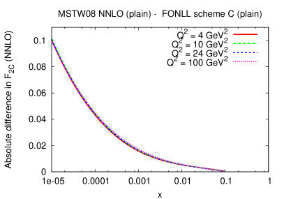
Let us be more precise about this latter point. The TR^′ scheme, discussed in Sect. 22.3.2, defines the default prescription from Ref. [469]. By construction, at NLO it should be similar for $F_{2c}$ to the S-ACOT-$\chi$ scheme and correspondingly also to FONLL-A (when the same form of $\chi$-scaling threshold prescription is used consistently in all cases). The only difference is the additional (subleading) ${\cal O}(\alpha_{s}^{2})$ contribution which is a constant for $Q^{2}/m_{c}^{2}\to\infty$, and which is numerically significant for low $Q^{2}$. This leads to a slightly larger $F_{2c}$, though the relative difference disappears as $Q^{2}/m_{c}^{2}\to\infty$.

On the other hand, the NNLO definition in TR^′ should be the same for $F_{2c}$ as in FONLL-C up to the additional ${\cal O}(\alpha_{s}^{3})$ term from the massive coefficient function, which stems from the matching between the massive and GM schemes at $Q^{2}=m_{c}^{2}$, provided that as usual the threshold prescription is the same is both cases. These expectations are explicitly verified both at NLO and at NNLO in Figs. 64-65.

Finally, the NLO TR^′ will be the same as the FONLL-B scheme only at $Q^{2}=m_{c}^{2}$ and will differ from it for any other value $Q^{2}>m_{c}^{2}$, since the ${\cal O}(\alpha_{s}^{2})$ term included in both cases is frozen at $Q^{2}=m_{c}^{2}$ in TR^′ but runs as usual with $Q^{2}$ in FONLL-B. As noted earlier, both TR^′ and FONLL-B schemes at high $Q^{2}$ contain strictly higher order (beyond ${\cal O}(\alpha_{s})$) terms which are of the form $\alpha^{2}_{s}(m_{c}^{2})g(m_{c}^{2})$ in the former case and $\alpha^{2}_{s}(Q^{2})g(Q^{2})$ in the latter case (with analogous singlet quark terms). These turn out to be of opposite sign in the two cases although they both originate from the order $\alpha_{s}^{2}$ massive coefficient functions.

Note that this implies that NLO TR^′ is, as discussed before, identical to S-ACOT and FONLL-A up to a constant subleading term. In particular, the same non-negligible dependence on the choice of threshold prescription which is present in S-ACOT and FONLL-A will be present in NLO TR^′. This is opposite to what happens for FONLL-B, since as discussed extensively in Ref. [473], in this case the matched results turns out to be essentially independent of the choice of arbitrary threshold prescription, and the FONLL result coincides with the massive result for low and moderate $Q^{2}$.

A variety of modifications of the default TR^′ scheme have been explored in Ref. [487], along with their consequences, and a new “optimal choice” suggested. In particular, the higher order FF part was frozen in the original TR definition in order to obtain the exact continuity of the evolution of $F_{2}$, but this is not required in the TR^′ definition. Allowing this term instead to fall like a power of $Q^{2}$ results in exactly the same results as S-ACOT or FONLL-A (or FONLL-C at NNLO) in the limit that $Q^{2}/m_{c}^{2}\to\infty$, where those terms causing the differences in the default scheme now vanish.

After this detailed discussion about the comparison for $F_{2c}$ between the FONLL and TR^′ schemes, we now turn to discuss the results of the comparison for the longitudinal structure function $F_{Lc}$. These results are shown in Figs. 66-67. In this case, due to the perturbative ordering of the TR/TR^′ schemes, FONLL-B turns out to be very similar to TR^′ NLO (which now includes also the full running $\alpha_{s}^{2}$ massive term) for any $Q^{2}$. In the case of the NNLO schemes, FONLL-C is somewhat different to TR^′ NNLO. This is likely due to the additional $\alpha_{s}^{3}$ term included in the latter. Differences tend to wash out with $Q^{2}$, but an order $\alpha_{s}^{3}$ discrepancy, depending on the massless coefficient functions at this order, persists even at high $Q^{2}$.

Figure 62: The $F_{2c}$ structure function for $Q^{2}=4$ and 10 GeV² in FONLL and in TR^′, both for the NLO schemes (left plots) and for the NNLO schemes (right plots). In both cases the default threshold prescriptions are used: $\chi$-scaling using Eq. 95 for TR^′ and a damping factor for FONLL.

Figure 63: Same as Fig. 62 for $Q^{2}=24$ and 100 GeV².

Figure 64: Same as Fig. 62 with all threshold prescriptions switched off in the FONLL and TR^′ schemes.

Figure 65: Same as Fig. 63 with all threshold prescriptions switched off in the FONLL and TR^′ schemes.

Figure 66: The $F_{Lc}$ structure function for $Q^{2}=4$ and 10 GeV² from FONLL and TR^′, both for the NLO schemes (left plots) and for the NNLO schemes (right plots).

Figure 67: Same as Fig. 66 for $Q^{2}=24$ and 100 GeV².

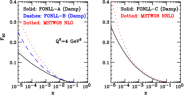
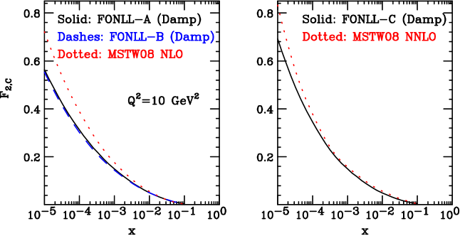
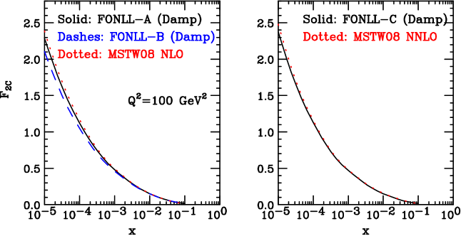
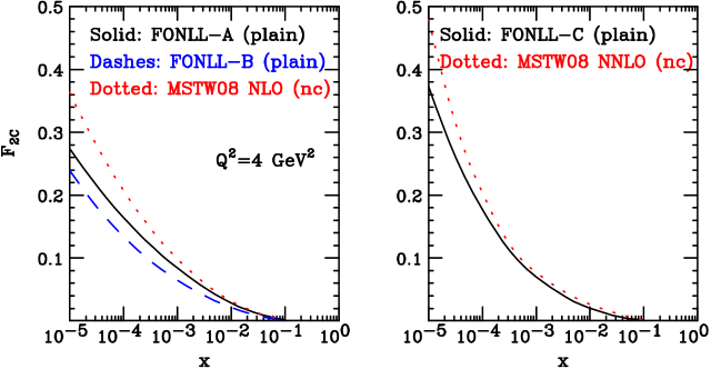
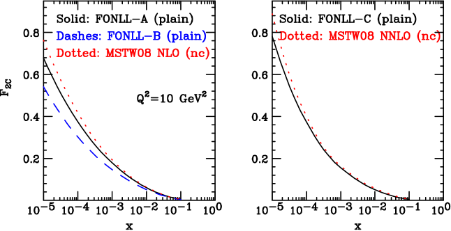
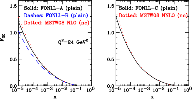
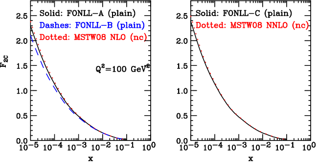
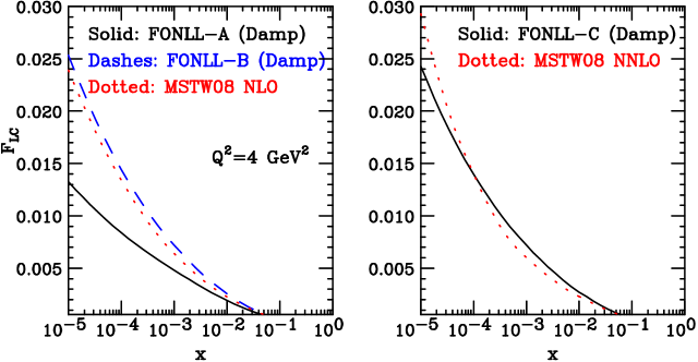
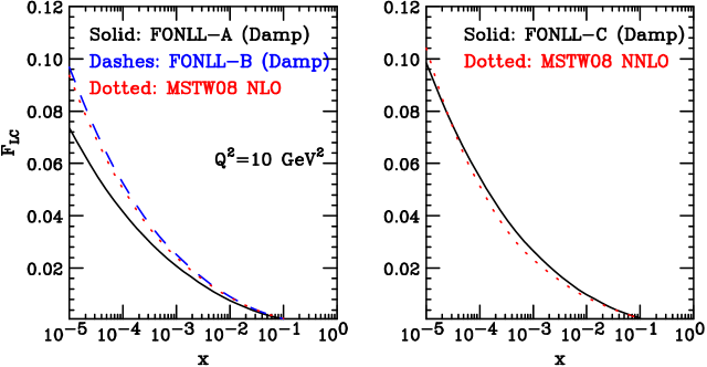
22.5 Conclusions

In this contribution we have performed a detailed quantitative comparison between GM-VFN heavy quark schemes in deep-inelastic scattering. We have compared the heavy quark schemes adopted by the three main global PDF fitting groups. The main results of this benchmark comparison have been the following:

1. FONLL-A (plain) is identical to S-ACOT, and FONLL-A-$\chi$ is identical to S-ACOT-$\chi$, both for $F_{2c}$ and $F_{Lc}$, when the same $\chi-$scaling threshold prescription is used in both cases.

2. The only difference between FONLL-A (plain) (and S-ACOT) and TR^′ NLO for $F_{2c}$ is a subleading $Q^{2}$-independent matching term present in the TR^′ scheme, whose relative impact decreases with $Q^{2}$.

3. Similarly, the only difference between FONLL-C (plain) and TR^′ NNLO for $F_{2c}$ is a subleading $Q^{2}$-independent matching term present in TR^′.

4. FONLL scheme B is only identical to TR^′ NLO for $F_{2c}$ for $Q^{2}=m_{c}^{2}$, being different for any other $Q^{2}>m_{c}^{2}$, since the higher order term included in TR^′ is frozen at the heavy quark threshold.

5. FONLL-B, as discussed in Ref. [473], is to a very good approximation (to the order $\alpha_{S}^{2}$ massive result as $Q^{2}$ increases above $m_{c}^{2}$) independent of the choice of arbitrary threshold prescription. The other NLO schemes, S-ACOT, TR^′ NLO and FONLL-A are, on the other hand, much more sensitive to this choice, with differences that can be as large as the effect of the resummation itself.

6. Only the ACOT type (ACOT, S-ACOT, S-ACOT-$\chi$) and the FONLL-A schemes reduce to exactly the order $\alpha_{S}$ NLO massless limit at high $Q^{2}$, without some strictly higher-order $\alpha_{S}^{2}$ contributions.

7. Due to the TR ordering, FONLL scheme B is very close to TR^′ NLO for the case of the longitudinal structure function $F_{Lc}$.

In order to provide easy access to the present benchmark comparisons for future developments, we have summarized the values of the DIS charm structure function $F_{2c}$ at the benchmark kinematical points obtained from the various possible approaches discussed in the text. The benchmark tables for the FONLL schemes are given in Tables 15 and 16, those of the ACOT scheme in Table 17, and finally those of the TR^′ schemes in Table 18.

Whenever new or improved GM-VFN schemes are proposed, they should be compared with the results of these benchmark tables, in order to quantitatively compare with previous approaches and avoid confusion. The corresponding benchmark numbers for the $F_{Lc}$ charm structure function are available from the authors upon request.

$x$	FONLL-A plain	FONLL-A-damp	FONLL-A-$\chi$	FONLL-B plain	FONLL-B-damp	FONLL-B-$\chi$
$Q^{2}=4$ GeV2
$10^{-5}$	0.27426	0.15066	0.15220	0.23919	0.24905	0.25011
$10^{-4}$	0.16424	0.09356	0.09273	0.13421	0.13606	0.13672
$10^{-3}$	0.08424	0.05055	0.04875	0.06483	0.06375	0.06391
$10^{-2}$	0.02859	0.01738	0.01591	0.02161	0.02063	0.02058
$10^{-1}$	0.00207	0.00072	0.00031	0.00093	0.00068	0.00059
$Q^{2}=10$ GeV2
$10^{-5}$	0.67714	0.56354	0.51346	0.54126	0.55361	0.56340
$10^{-4}$	0.37430	0.31206	0.28187	0.30220	0.30225	0.30449
$10^{-3}$	0.17900	0.14995	0.13374	0.14685	0.14405	0.14330
$10^{-2}$	0.06051	0.05056	0.04357	0.05196	0.05016	0.04913
$10^{-1}$	0.00562	0.00423	0.00252	0.00430	0.00392	0.00346
$Q^{2}=24$ GeV2
$10^{-5}$	1.19978	1.13985	1.08785	1.02189	1.02970	1.04182
$10^{-4}$	0.63020	0.59690	0.56568	0.55006	0.54938	0.55112
$10^{-3}$	0.28826	0.27221	0.25568	0.25873	0.25637	0.25476
$10^{-2}$	0.09642	0.09051	0.08307	0.09010	0.08869	0.08716
$10^{-1}$	0.00997	0.00908	0.00708	0.00924	0.00895	0.00831
$Q^{2}=100$ GeV2
$10^{-5}$	2.29879	2.28636	2.27201	2.10444	2.10708	2.11399
$10^{-4}$	1.13024	1.12186	1.11165	1.04894	1.04875	1.05111
$10^{-3}$	0.48483	0.48008	0.47343	0.46063	0.45974	0.45920
$10^{-2}$	0.15406	0.15207	0.14862	0.15111	0.15051	0.14962
$10^{-1}$	0.01646	0.01615	0.01510	0.01639	0.01627	0.01588

Table 15: Results of the benchmark comparison for the $F_{2c}(x,Q^{2})$ structure function in the two NLO FONLL schemes, denoted by scheme A and scheme B. In the two cases we provide the results without threshold prescription and with two different threshold prescriptions, $\chi-$scaling and a damping factor. Results are provided at the benchmark kinematical points in $x,Q^{2}$.

$x$	FONLL-C plain	FONLL-C-damp	FONLL-C-$\chi$
$Q^{2}=4$ GeV2
$10^{-5}$	0.37255	0.27609	0.27096
$10^{-4}$	0.17702	0.14585	0.14235
$10^{-3}$	0.07001	0.06492	0.06381
$10^{-2}$	0.02027	0.02004	0.02019
$10^{-1}$	0.00149	0.00078	0.00069
$Q^{2}=10$ GeV2
$10^{-5}$	0.78141	0.69206	0.64037
$10^{-4}$	0.37400	0.34507	0.32514
$10^{-3}$	0.15564	0.14932	0.14446
$10^{-2}$	0.05106	0.04938	0.04869
$10^{-1}$	0.00547	0.00462	0.00387
$Q^{2}=24$ GeV2
$10^{-5}$	1.30170	1.25019	1.19206
$10^{-4}$	0.63138	0.61466	0.59361
$10^{-3}$	0.26822	0.26401	0.25864
$10^{-2}$	0.09009	0.08856	0.08717
$10^{-1}$	0.01067	0.01012	0.00915
$Q^{2}=100$ GeV2
$10^{-5}$	2.39198	2.37634	2.35015
$10^{-4}$	1.13357	1.12863	1.11943
$10^{-3}$	0.47207	0.47058	0.46798
$10^{-2}$	0.15213	0.15146	0.15054
$10^{-1}$	0.01804	0.01784	0.01729

Table 16: Results of the benchmark comparison for the $F_{2c}(x,Q^{2})$ structure function in the NNLO FONLL scheme, denoted by scheme C. As before, we provide the results without threshold prescription and with two different threshold prescriptions, $\chi-$scaling and a damping factor.

$x$	S-ACOT plain	S-ACOT-$\chi$	S-ACOT-$\chi$ (v2)	Full ACOT plain
$Q^{2}=4$ GeV2
$10^{-5}$	0.27339	0.15780	0.23670	0.30121
$10^{-4}$	0.16327	0.09171	0.13749	0.17774
$10^{-3}$	0.08386	0.04497	0.06734	0.08956
$10^{-2}$	0.02839	0.01360	0.02030	0.02950
$10^{-5}$	0.00203	0.00026	0.00038	0.00169
$Q^{2}=10$ GeV2
$10^{-5}$	0.67349	0.52648	0.63177	0.69789
$10^{-4}$	0.37254	0.28768	0.34503	0.38545
$10^{-3}$	0.17826	0.13482	0.16153	0.18395
$10^{-2}$	0.06024	0.04338	0.05185	0.06211
$10^{-5}$	0.00554	0.00259	0.00305	0.00547
$Q^{2}=24$ GeV2
$10^{-5}$	1.19413	1.07983	1.16981	1.20362
$10^{-4}$	0.62805	0.56516	0.61188	0.63403
$10^{-3}$	0.28739	0.25642	0.27736	0.29070
$10^{-2}$	0.09588	0.08382	0.09046	0.09742
$10^{-5}$	0.00986	0.00736	0.00785	0.00997
$Q^{2}=100$ GeV2
$10^{-5}$	2.29983	2.25162	2.29665	2.29853
$10^{-4}$	1.12920	1.10453	1.12588	1.12988
$10^{-3}$	0.48339	0.47203	0.48072	0.48442
$10^{-2}$	0.15346	0.14918	0.15161	0.15415
$10^{-5}$	0.01629	0.01531	0.01540	0.01640

Table 17: Results of the benchmark comparison for the $F_{2c}(x,Q^{2})$ structure function for the ACOT family of NLO GM-VFN schemes. We provide the results for both full ACOT and simplified ACOT (S-ACOT) without any threshold prescriptions, as well as those for S-ACOT-$\chi$ with the $\chi-$scaling threshold prescription of Eq. 94, and S-ACOT-$\chi$ (v2) with the $\chi-$scaling threshold prescription of Eq. 95, Results are provided at the benchmark kinematical points in $x,Q^{2}$.

$x$	MSTW08 NLO plain	MSTW08 NLO $\chi$	MSTW08 NNLO plain	MSTW08 NNLO $\chi$
$Q^{2}=4$ GeV2
$10^{-5}$	0.36337	0.32667	0.47899	0.42824
$10^{-4}$	0.20751	0.18173	0.20366	0.18164
$10^{-3}$	0.09873	0.08220	0.07654	0.07139
$10^{-2}$	0.03174	0.02364	0.02649	0.02690
$10^{-1}$	0.00215	0.00046	0.00192	0.00128
$Q^{2}=10$ GeV2
$10^{-5}$	0.76342	0.72170	0.88803	0.83214
$10^{-4}$	0.41689	0.38936	0.40160	0.37813
$10^{-3}$	0.19326	0.17652	0.16315	0.15704
$10^{-2}$	0.06370	0.05530	0.05738	0.05679
$10^{-1}$	0.00571	0.00319	0.00575	0.00468
$Q^{2}=24$ GeV2
$10^{-5}$	1.28397	1.25966	1.40641	1.36811
$10^{-4}$	0.67251	0.65634	0.65687	0.64135
$10^{-3}$	0.30255	0.29252	0.27505	0.27089
$10^{-2}$	0.09946	0.09403	0.09593	0.09520
$10^{-1}$	0.01008	0.00806	0.01090	0.00998
$Q^{2}=100$ GeV2
$10^{-5}$	2.38877	2.38560	2.49312	2.47939
$10^{-4}$	1.17358	1.17027	1.16278	1.15769
$10^{-3}$	0.49872	0.49601	0.47953	0.47822
$10^{-2}$	0.15719	0.15534	0.15837	0.15802
$10^{-1}$	0.01658	0.01568	0.01836	0.01789

Table 18: Results of the benchmark comparison for the $F_{2c}(x,Q^{2})$ structure function for the NLO and NNLO TR^′ schemes. In the two cases we provide the results without threshold prescription and with the TR^′ $\chi-$scaling threshold prescription which is implemented in the MSTW08 parton fits. Results are provided at the benchmark kinematical points in $x,Q^{2}$.

Part IV HIGGS PHENOMENOLOGY

23 ADDITIONAL JET PRODUCTION FROM HIGGS BOSON + DIJETS THROUGH GLUON FUSION

23.1 Introduction

The description of Higgs production in association with jets, through gluon fusion, is important for several reasons. Firstly, a clean extraction of the coupling of the Higgs boson to weak bosons in the weak-boson-fusion channel requires that the gluon fusion contribution be suppressed as much as possible. Secondly, by focusing directly on the gluon fusion contribution, it is possible to extract not just the absolute size, but also the $CP$-structure of the Higgs boson coupling to gluons induced through a top-loop[488]. In both cases the description of further hard radiation from the lowest-order process is important. The different radiation pattern observed in weak-boson-fusion and gluon-fusion can be used to reject the latter. Moreover, the tree-level observations on the extraction of $CP$-properties could be spoilt by decorrelations due to further hard emissions, unless observables which are robust against these higher order corrections are employed in the analysis[489].

In this contribution we will compare the description of the final state obtained using a tree-level matched parton shower [269, 270, 271] (represented by SHERPA [131, 132]), a next-to-leading order (NLO) calculation of $hjj$ production through gluon fusion (as implemented in MCFM[8, 490]) and finally the HEJ (High Energy Jets) resummation scheme based on the factorisation of scattering amplitudes in the high energy limit[345, 346, 347, 348].

23.2 Inclusive predictions

We start by comparing predictions for distributions in a sample obtained by requiring at least two jets of at least 40 GeV transverse momentum and a rapidity less then 4.5 obtained with the $k_{t}$-jet algorithm of Ref.[491] with $D=0.7$. The rapidity of the Higgs boson is also required to be less then 4.5. For this study we have chosen a putative Higgs boson mass of 120 GeV and set the centre-of-mass energy, $\sqrt{s}=10$ TeV.

Figure 68: The distribution with respect to the rapidity difference $\Delta y_{ab}$ between the most forward and most backward jet of more than 40 GeV.

Figure 69: The average number of hard jets (above 40 GeV transverse momentum) obtained in the $k_{t}$ jet algorithm, as a function of the largest rapidity span $\Delta y_{ab}$ between two jets.

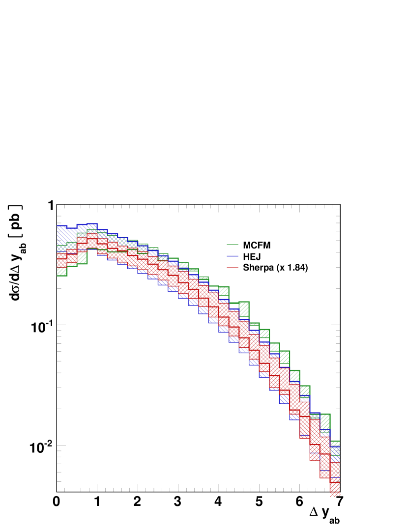
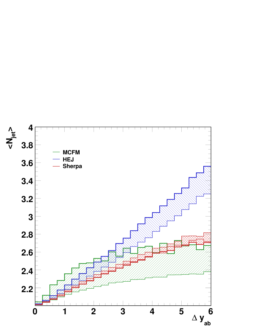
In Fig. 69 we compare the differential distribution of the rapidity span between the most forward and most backward jet, $\Delta y_{ab}$, obtained within the three descriptions. For MCFM and HEJ the bands indicate the variation obtained by changing the renormalisation and factorisation scale between 40 GeV and 120 GeV (but with two powers of $\alpha_{s}$ always evaluated at the scale of the Higgs boson mass). The uncertainty of the predictions made with SHERPA is estimated by varying the prefactor of the nodal scales within the parton shower (and the higher-order tree-level matrix elements) between 1/2 and 2. We see that the shapes are all in good agreement with each other, and that the scale uncertainty is smallest for the full NLO calculation of MCFM.

In Fig. 69 we analyse directly the average number of hard jets (above 40 GeV transverse momentum) obtained in the $k_{t}$ jet algorithm as a function of the rapidity span $\Delta y_{ab}$. The same observable was analysed for $W+$dijets in Ref.[492]. As discussed there, the framework of Ref.[339, 340, 341] implies, for a certain class of processes (to which both $pp\to hjj$ through gluon fusion and $pp\to Wjj$ belong), an increase in jet count with increasing rapidity span. In turn, such an increase in the amount of hard radiation necessitates the inclusion of increasingly higher order corrections in order to obtain stable predictions for increasing $\Delta y_{ab}$. The modelling of this increase is important for the application of a jet veto to suppress the gluon fusion contribution to $h+$dijets. While all three calculations show an increase of the jet count with increasing $\Delta y_{ab}$, the amounts of increase differ. Using HEJ, the average number of jets found in events with a rapidity span of 5 is just slightly more than 3 (compared to 2.8 in the case of $W+$dijets studied in Ref.[492]). SHERPA produces less of the hard radiation, with an average of 2.8 hard jets when the rapidity span is $\Delta y_{ab}=5$. The rise in the average number of jets with increasing rapidity span obtained with SHERPA is slightly slower than linear – and slower than the predictions obtained with ALPGEN[353]+HERWIG[351] for $W+$dijets. Finally, the prediction of NLO QCD (obtained from MCFM) indicates an even smaller average number of jets at large rapidity spans. For a scale choice of 40 GeV, the average number of hard jets in events with a span of 5 units of rapidity is comparable to that obtained in NLO QCD for $W$+dijets[492]. There is a large variation induced by a variation of factorisation and renormalisation scale, which is to be expected since this observable only becomes non-trivial at NLO. This variation is particularly noticeable at small rapidity spans, where the extrema of the band represent rises that are either stronger or weaker than those obtained in the other two predictions.

23.3 Predictions at large rapidity span

We now impose an additional cut, to focus on the region where two of the jets are separated by a large rapidity span, $\Delta y_{ab}>4$. This situation arises naturally for the weak-boson-fusion process, where the gluon-fusion channel discussed here will act as a background in extracting the coupling between the weak and the Higgs boson.

Figure 70: The transverse momentum of the Higgs boson, in the region of large jet rapidity span between two jets defined by $\Delta y_{ab}>4$. The inset shows the same quantity on a linear scale, over a smaller range.

Figure 71: Dependence of the normalized cross section on the jet veto parameter $y_{c}$, defined in the text. For large $y_{c}$ this normalized cross section gives the prediction for the ratio of exclusive dijet and inclusive dijet+X cross sections.

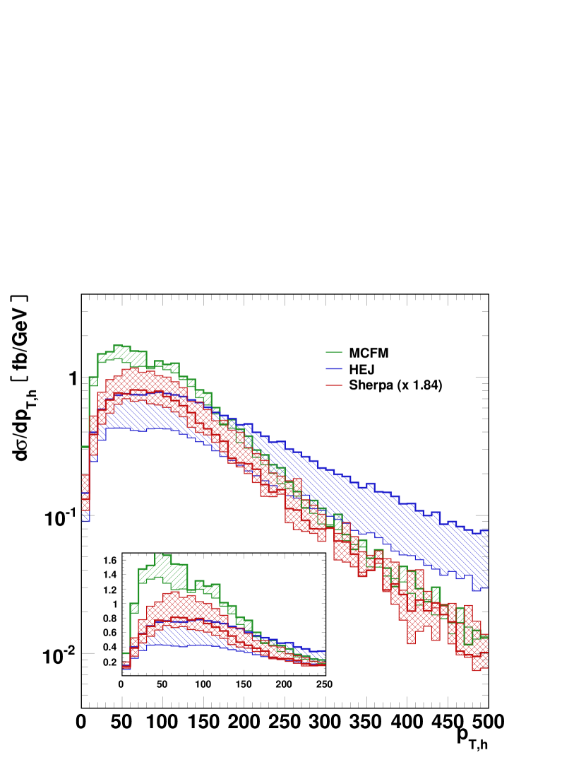
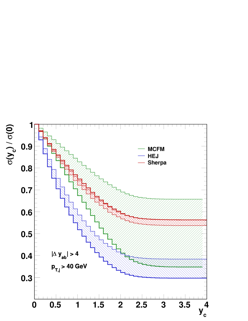
In Fig. 71 we show the predictions for the transverse momentum spectrum of the Higgs boson. The HEJ approach predicts a much harder spectrum than that obtained in SHERPA and MCFM. As expected, the latter two predictions agree with each other quite well in this region, with the NLO curve consistently narrower.

Finally, in Fig. 71 we investigate the effect of vetoing additional jet activity beyond the two that define the rapidity span. This is interesting for suppressing the gluon-fusion contribution. We parametrize the veto as in Ref. [346] by using the variable $y_{c}$ as follows. Given the rapidity span $\Delta y_{ab}=|y_{a}-y_{b}|$, we compute the midpoint of rapidities of the two jets furthest apart in rapidity, $y_{0}=(y_{a}+y_{b})/2$. An event is only removed by the veto if it contains a further jet (with transverse momentum at least 40 GeV) at rapidity $y^{\prime}$ with $|y^{\prime}-y_{0}|<y_{c}$. With this definition we see that the cross section $\sigma(y_{c}=0)$ corresponds to applying no veto at all, whilst the limit of large $y_{c}$ corresponds to vetoing all additional jets. The $y$-axis on Fig. 71 indicates the fraction of the cross section with no jet-veto which survives as a function of $y_{c}$. Once more there is a clear difference between the HEJ prediction and that of SHERPA and MCFM, both in the dependence on $y_{c}$ as it increases from zero, and in the asymptotic value for large $y_{c}$. This is simply a reflection of the differences observed in the predictions for the amount of hard jets for larger rapidity spans, as indicated in Fig. 69. As in that figure, the MCFM band indicates a large scale uncertainty due to the essentially leading order nature of the prediction for this observable.

23.4 Conclusions

In this contribution we have performed an introductory study of the additional radiation expected in Higgs + dijet events at the LHC. Understanding the characteristics of this radiation would be crucial to determining the nature of the Higgs boson, such as its couplings to matter and its $CP$-properties. We have compared the predictions of three very different theoretical approaches: a matrix-element improved parton-shower (SHERPA), NLO QCD (MCFM) and a calculation based on behaviour of the matrix elements to all orders in the high energy limit (the HEJ resummation).

The predictions obtained for the rapidity difference between the most forward and most backward hard jet are in good agreement between all three calculations. Furthermore, the predictions for the number of additional jets are in reasonable agreement between the models for smaller rapidity spans (up to 2). For larger rapidity spans, the HEJ resummation scheme leads to more hard jets than in either NLO QCD or SHERPA. This induces a difference in the effect of a veto on further jet activity. Using HEJ, the Higgs boson tends to be accompanied by more additional central radiation that would be subject to a jet veto.

The work presented here should be contrasted with the similar study of $W+$dijet events in Ref.[492]. A more detailed analysis of predictions for additional radiation in $W$, $Z$ and $h$+dijet events is required in order to assess the potential for applying results from the study of $W$,$Z$+dijets to that of $h$+dijets. One might expect that a relatively early study of radiation in $W$ and $Z$+dijet events could pave the way for later studies of the Higgs boson with more integrated luminosity.

24 NLO ELECTROWEAK CORRECTIONS TO HIGGS BOSON PRODUCTION AT HADRON COLLIDERS: TOWARDS A FULL COMPLEX MASS SCHEME

24.1 NLO Electroweak for $gg\to H$

Gluon fusion is the main production channel for the Standard Model Higgs boson at hadron colliders. Unsurprisingly, radiative corrections have been thoroughly investigated in the past years; in particular, since next-to-leading order (NLO) QCD corrections increase the inclusive cross section for Higgs production at the LHC by a factor of about $1.5$ to $1.7$ with respect to the leading order (LO) term [309], there was a flurry of activity on higher order QCD effects. Recent reviews on the subject can be found in Refs. [493, 494, 316, 495], Refs. [496, 497, 498] We have recently completed the evaluation of all NLO electroweak corrections to the gluon-fusion Higgs production cross section at the partonic level in Refs. [499, 500, 501, 502]. The inclusive cross section for the production of the Standard Model Higgs boson in hadronic collisions can be written as

$$\sigma\left(s,M^{2}_{{}_{H}}\right) = \sum_{i,j}\,\int_{0}^{1}\!dx_{1}\int_{0}^{1}\!dx_{2}\,\,f_{i/h_{1}}\left(x_{1},\mu^{2}_{{\scriptscriptstyle{F}}}\right)\,f_{j/h_{2}}\left(x_{2},\mu^{2}_{{\scriptscriptstyle{F}}}\right)\,\times$$ (97)

$$\times \int_{0}^{1}\!dz\,\delta\left(z-\frac{M^{2}_{{}_{H}}}{s\,x_{1}x_{2}}\right)\,z\,\sigma^{(0)}\,G_{ij}\left(z;\alpha_{{\scriptscriptstyle{S}}}(\mu^{2}_{{\scriptscriptstyle{R}}}),M^{2}_{{}_{H}}/\mu^{2}_{{\scriptscriptstyle{R}}};M^{2}_{{}_{H}}/\mu^{2}_{{\scriptscriptstyle{F}}}\right),$$

where $\sqrt{s}$ is the center-of-mass energy and $\mu_{{\scriptscriptstyle{F}}}$ and $\mu_{{\scriptscriptstyle{R}}}$ stand for factorization and renormalization scales. In Eq.(97) the partonic cross section for the sub-process $ij\to H+X$, with $i(j)=g,q_{f},{\bar{q}}_{f}$, has been convoluted with the parton densities $f_{a/h_{b}}$ for the colliding hadrons $h_{1}$ and $h_{2}$. The Born factor is $\sigma^{(0)}$. The coefficient functions $G_{ij}$ can be computed in QCD through a perturbative expansion in the strong-coupling constant $\alpha_{\scriptscriptstyle{S}}$,

$$G_{ij}\left(z;\alpha_{{\scriptscriptstyle{S}}}(\mu^{2}_{{\scriptscriptstyle{R}}}),M^{2}_{{}_{H}}/\mu^{2}_{{\scriptscriptstyle{R}}};M^{2}_{{}_{H}}/\mu^{2}_{{\scriptscriptstyle{F}}}\right)=\alpha_{{\scriptscriptstyle{S}}}^{2}(\mu^{2}_{{\scriptscriptstyle{R}}})\sum_{n=0}^{\infty}\left(\frac{\alpha_{{\scriptscriptstyle{S}}}(\mu^{2}_{{\scriptscriptstyle{R}}})}{\pi}\right)^{n}G_{ij}^{(n)}\left(z;M^{2}_{{}_{H}}/\mu^{2}_{{\scriptscriptstyle{R}}};M^{2}_{{}_{H}}/\mu^{2}_{{\scriptscriptstyle{F}}}\right),$$ (98)

with a scale-independent LO contribution given by $G^{(0)}_{ij}(z)=\delta_{ig}\,\delta_{jg}\,\delta\left(1-z\right).$ The inclusion of higher order electroweak corrections in Eq.(97) requires to define a factorization scheme. Originally, we introduced two options for replacing the purely QCD-corrected partonic cross section in Eq.(97) with the expression including NLO EW corrections, complete factorization: $\sigma^{(0)}\,G_{ij}\to\sigma^{(0)}\,\left(1+\delta_{\rm{\scriptscriptstyle{EW}}}\right)\,G_{ij}$; and partial factorization: $\sigma^{(0)}\,G_{ij}\to\sigma^{(0)}\,\Bigl{[}G_{ij}+\alpha_{\scriptscriptstyle{S}}^{2}(\mu^{2}_{{\scriptscriptstyle{R}}})\delta_{\rm{\scriptscriptstyle{EW}}}\,G^{(0)}_{ij}\Bigr{]}$, where $\delta_{\rm{\scriptscriptstyle{EW}}}$ embeds all NLO electroweak corrections to the partonic cross section $\sigma(gg\to H)$,

$$\sigma_{\rm{\scriptscriptstyle{EW}}}=\alpha_{{\scriptscriptstyle{S}}}^{2}(\mu^{2}_{{\scriptscriptstyle{R}}})\sigma^{(0)}(1+\delta_{\rm{\scriptscriptstyle{EW}}}),$$ (99)

The CF option amounts to an overall re-scaling of the QCD result, dressed at all orders with the NLO electroweak correction factor $\delta_{\rm{\scriptscriptstyle{EW}}}$; the PF option is equivalent to add electroweak corrections to QCD ones. Note that a calculation of the mixed QCD - EW corrections has been performed in Ref. [493]; a significant numerical difference from the prediction of the complete factorization hypothesis has not been observed. Results for NLO EW corrections are given in Fig. 72.

Figure 72: NLO electroweak percentage corrections to the partonic cross section $\sigma(g\,g\to H)$.

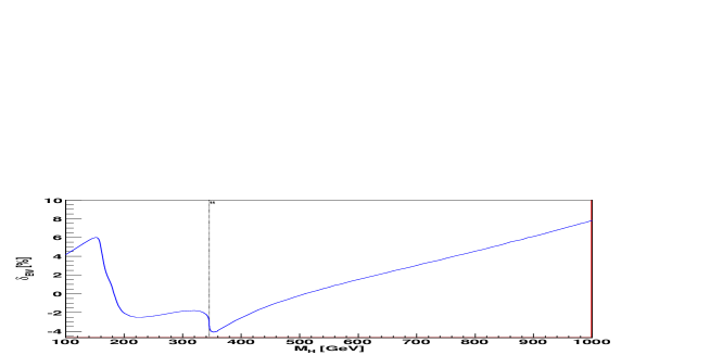
24.2 Higgs Pseudo-Observables

The Higgs boson, as well as the $W$ or $Z$ bosons, are unstable particles; as such they should be removed from in/out bases in the Hilbert space, without changing the unitarity of the theory. Concepts as the production of an unstable particle or its partial decay widths, not having a precise meaning, are only an approximation of a more complete description. The inconsistencies associated with the on-shell LSZ formulation of an unstable external particles become particularly severe starting from two-loops, as described in Ref. [500]. At the parton level the $S\,$-matrix for the process $i\to f$ can be written as

$$S_{fi}=V_{i}(s)\,\Delta_{{\scriptscriptstyle{H}}}(s)\,V_{f}(s)+B_{if}(s),$$ (100)

where $V_{i}$ is the production vertex $i\to H$ (e.g. $gg\to H$), $V_{f}$ is the decay vertex $H\to f$ (e.g. $H\to\gamma\gamma$), $\Delta_{{\scriptscriptstyle{H}}}$ is the Dyson re-summed Higgs propagator and $B_{if}$ is the non - resonant background (e.g. $gg\to\gamma\gamma$ boxes). In the next section we will introduce the notion of complex pole. A vertex is defined by the following decomposition

$$V_{f}(s)=\sum_{a}\,V^{a}_{f}\left(s\,,\,\{S\}\right)\,F^{a}_{f}\left(\{p_{f}\}\right)$$ (101)

where $s=-P_{{\scriptscriptstyle{H}}}^{2}$ (with $P_{{\scriptscriptstyle{H}}}=\sum_{f}p_{f}$), $s\,\oplus\,\{S\}$ is the set of Mandelstam invariants that characterize the process $H\to f$, $V^{a}_{f}$ are scalar form factors and the $F^{a}_{f}$ contain spinors, polarization vectors etc. Although a modification of the LSZ reduction formulas has been proposed long ago for unstable particles we prefer an alternative approach where one considers extracting informations on the Higgs boson directly from

$$<\,f\;{\rm out}\,|\,H\,>\,<\,H\,|\,i\;{\rm in}\,>+\sum_{n\,\not=\,H}\,<\,f\;{\rm out}\,|\,n\,>\,<\,n\,|\,i\;{\rm in}\,>,$$ (102)

for some initial state $i$ and some final state $f$ and where $\{n\}\,\oplus\,H$ is a complete set of states (not as in the in/out bases). The price to be paied is the necessity of moving into the complex plane. Define $s_{{\scriptscriptstyle{H}}}$ and $\Pi_{{\scriptscriptstyle{H}\scriptscriptstyle{H}}}(s)$ as

$$s_{{\scriptscriptstyle{H}}}-m^{2}_{{\scriptscriptstyle{H}}}+\Sigma_{{\scriptscriptstyle{H}\scriptscriptstyle{H}}}(s_{{\scriptscriptstyle{H}}})=0,\qquad\Pi_{{\scriptscriptstyle{H}\scriptscriptstyle{H}}}(s)=\frac{\Sigma_{{\scriptscriptstyle{H}\scriptscriptstyle{H}}}(s)-\Sigma_{{\scriptscriptstyle{H}\scriptscriptstyle{H}}}(s_{{\scriptscriptstyle{H}}})}{s-s_{{\scriptscriptstyle{H}}}},$$ (103)

where $\Sigma_{{\scriptscriptstyle{H}\scriptscriptstyle{H}}}$ is the Higgs self-energy; then the, Dyson re-summed, Higgs propagator becomes

$$\Delta_{{\scriptscriptstyle{H}\scriptscriptstyle{H}}}(s)=(s-s_{{\scriptscriptstyle{H}}})^{-1}\,\Bigl{[}1+\Pi_{{\scriptscriptstyle{H}\scriptscriptstyle{H}}}(s)\Bigr{]}^{-1},\qquad Z_{{\scriptscriptstyle{H}}}=1+\Pi_{{\scriptscriptstyle{H}\scriptscriptstyle{H}}}.$$ (104)

Using Eq.(104) we can write Eq.(100) as

$$S_{fi}=\Bigl{[}Z^{-1/2}_{{\scriptscriptstyle{H}}}(s)\,V_{i}(s)\Bigr{]}\,\frac{1}{s-s_{{\scriptscriptstyle{H}}}}\,\Bigl{[}Z^{-1/2}_{{\scriptscriptstyle{H}}}(s)\,V_{f}(s)\Bigr{]}+B_{if}(s).$$ (105)

From the $S\,$-matrix element for a physical process $i\to f$ we extract the relevant pseudo - observable,

$$S\left(H_{c}\to f\right)=Z^{-1/2}_{{\scriptscriptstyle{H}}}(s_{{\scriptscriptstyle{H}}})\,V_{f}(s_{{\scriptscriptstyle{H}}}),\quad S_{fi}=\frac{S\left(i\to H_{c}\right)\,S\left(H_{c}\to f\right)}{s-s_{{\scriptscriptstyle{H}}}}+\hbox{non resonant terms}.$$ (106)

which is gauge parameter independent by construction. The partial decay width is further defined as

$$M_{{\scriptscriptstyle{H}}}\,\Gamma\left(H_{c}\to f\right)=\frac{(2\,\pi)^{4}}{2}\,\int\,d\Phi_{f}\left(P_{{\scriptscriptstyle{H}}}\,,\,\{p_{f}\}\right)\,\sum_{\rm spins}\,\Bigr{|}S\left(H_{c}\to f\right)\Bigr{|}^{2},$$ (107)

where the integration is over the phase space spanned by $|f>$, with the constraint $P_{{\scriptscriptstyle{H}}}=\sum\,p_{f}$. One should not confuse phase space and the real value of $s=-P^{2}_{{\scriptscriptstyle{H}}}$ where the realistic observable is measured with the complex value for $s$ where to compute gauge invariant loop corrections. The choice of $P^{2}_{{\scriptscriptstyle{H}}}$ (phase space) where to define the pseudo - observable is conventional and we will use $M^{2}_{{\scriptscriptstyle{H}}}=\mid s_{{\scriptscriptstyle{H}}}\mid$, with $s_{{\scriptscriptstyle{H}}}=\mu^{2}_{{\scriptscriptstyle{H}}}-i\,\mu_{{\scriptscriptstyle{H}}}\,\gamma_{{\scriptscriptstyle{H}}}$.

We define two different schemes and compare their results: the CMRP scheme [500], the complex mass scheme with complex internal $W$ and $Z$ poles; the CMCP scheme, the (complete) complex mass scheme with complex, external, Higgs ($W,Z$ etc.) where the LSZ procedure is carried out at the Higgs complex pole (on the second Riemann sheet). We present the ratio of $\sigma(pp\to H)$ in the two schemes, using MSTW 2008 LO partondistribution functions (PDF) [449]. The ratio is given in Fig. 73.

Figure 73: The ratio $\sigma_{\rm{\scriptscriptstyle{CMCP}}}/\sigma_{\rm{\scriptscriptstyle{CMRP}}}$ for the production cross-section $pp\to H$, as a function of $\mu_{{\scriptscriptstyle{H}}}$, for different energies, $\sqrt{s}=3\,$TeV (red), $\sqrt{s}=10\,$TeV (blue) and $\sqrt{s}=14\,$TeV (yellow). Cross-sections are computed with MSTW2008 LO PDFs.

ACKNOWLEDGEMENTS

I gratefully acknowledge the unvaluable assistance of Christian Sturm and Sandro Uccirati in all steps of this project.

25 QCD-ELECTROWEAK EFFECTS AND A NEW PREDICTION FOR HIGGS PRODUCTION IN GLUON FUSION WITHIN THE SM

25.1 Introduction

The search for the Higgs boson is a primary goal of the CERN Large Hadron Collider (LHC), and is a central part of Fermilab’s Tevatron program. Recently, the Tevatron collaborations reported a 95% confidence level exclusion of a Standard Model Higgs boson with a mass in the range $163-166\,{\rm GeV}$ [503].
The dominant production mode at both colliders, gluon fusion through top-quark loops, receives important QCD radiative corrections [310, 504, 309]. The inclusive result increases by a factor of 2 at the LHC and 3.5 at the Tevatron when perturbative QCD effects through next-to-next-to-leading order (NNLO), in the infinite top quark mass limit, are taken into account [312, 311]. A review of the latest theoretical developments in the search for the Higgs boson within the Standard Model can be found in [505] . The theoretical uncertainty from effects beyond NNLO is estimated to be about $\pm 10\%$ by varying renormalization and factorization scales. At this level of precision, electroweak corrections to the Higgs signal become important. In Ref. [506, 507], the authors pointed out the importance of a subset of diagrams where the Higgs couples to the W and Z gauge bosons which subsequently couple to light quarks. A careful study of the full 2-loop electroweak effects was performed in Ref. [501]. They increase the leading-order cross section by up to $5-6\%$ for relevant Higgs masses. An important question is whether these light-quark contributions receive the same QCD enhancement as the top quark loops. If they do, then the full NNLO QCD result is shifted by $+5-6\%$ from these electroweak corrections. As this effect on the central value of the production cross section and therefore on the exclusion limits and future measurements is non-negligible, it is important to quantify it. The exact computation of the mixed electroweak/QCD effects needed to do so requires 3-loop diagrams with many kinematic scales, and 2-loop diagrams with four external legs for the real-radiation terms. Such a computation is prohibitively difficult with current computational techniques.
In Ref. [493], the QCD corrections to the light-quark terms in the Higgs production cross section via gluon fusion were computed using an effective theory approach. This approach was rigorously justified by applying a hard-mass expansion procedure to the full 3-loop corrections. In addition to that, the most up-to-date QCD prediction for the Higgs boson production cross section in this channel was provided for use in setting Tevatron exclusion limits. This includes the MSTW2008 PDFs, the exact NLO K-factors for the top, top-bottom interference and bottom quark contributions, NLO effects arising from W and Z gauge bosons [508] and all the new theoretical results.

25.2 The mixed QCD-electroweak effects

The cross section for Higgs boson production in hadronic collisions can be written as

$$\sigma(s,M_{H}^{2}) = \sum_{i,j}\int_{0}^{1}dx_{1}\int_{0}^{1}dx_{2}\,f_{i/h_{1}}(x_{1},\mu_{F}^{2})f_{j/h_{2}}(x_{2},\mu_{F}^{2})\int_{0}^{1}dz\,\delta\left(z-\frac{M_{H}^{2}}{x_{1}x_{2}s}\right)$$ (108)

$$\times z\,\hat{\sigma}_{ij}\left(z;\alpha_{s}(\mu_{R}^{2}),\alpha_{EW},M_{H}^{2}/\mu_{R}^{2};M_{H}^{2}/\mu_{F}^{2}\right).$$

Here, $\sqrt{s}$ is the center-of-mass energy of the hadronic collision, $\mu_{R}$ and $\mu_{F}$ respectively denote the renormalization and factorization scales, and the $f_{i/h}$ denote the parton densities. The quantity $z\hat{\sigma}$ is the partonic cross section for the process $ij\to H+X$ with $i,j=g,q,\bar{q}$. As indicated, it admits a joint perturbative expansion in the strong and electroweak couplings. Considering QCD and electroweak corrections and suppressing the scale dependence for simplicity, the partonic cross section can be written as:

$$\hat{\sigma}_{ij}=\sigma^{(0)}_{\rm EW}\,G^{(0)}_{ij}\left(z\right)+\sigma^{(0)}\sum_{n=1}^{\infty}\left(\frac{\alpha_{s}}{\pi}\right)^{n}G^{(n)}_{ij}(z).$$ (109)

The QCD corrections to the one-loop diagrams coupling the Higgs boson to gluons via a top-quark loop are given by

$$G_{ij}(z;\alpha_{s})=\sum_{n=1}^{\infty}\left(\frac{\alpha_{s}}{\pi}\right)^{n}G^{(n)}_{ij}(z).$$ (110)

The cross section in Eq. (109) includes corrections to the leading-order result valid through ${\cal O}(\alpha)$ in the electroweak couplings and to ${\cal O}(\alpha_{s}^{2})$ in the QCD coupling constant in the large top-mass limit upon inclusion of the known results for $G^{(1,2)}_{ij}$. Since the perturbative corrections to the leading-order result are large, it is important to quantify the effect of the QCD corrections on the light-quark electroweak contributions. This would require knowledge of the mixed ${\cal O}(\alpha\alpha_{s})$. In lieu of such a calculation, the authors of Ref. [501] studied two assumptions for the effect of QCD corrections on the 2-loop light-quark diagrams.

• Partial factorization: no QCD corrections to the light-quark electroweak diagrams are included. With this assumption, electroweak diagrams contribute only a $+1-2\%$ increase to the Higgs boson production cross section.

• Complete factorization: the QCD corrections to the electroweak contributions are assumed to be identical to those affecting the heavy-quark diagrams.

In this case the light-quark diagrams increase the full NNLO QCD production cross section by $+5-6\%$. The last assumption was used in earlier exclusions of a SM Higgs boson by the Tevatron collaborations. The calculation of the ${\cal O}(\alpha\alpha_{s})$, which allows one to check these assumptions, can be done in the framework of an effective field theory where the W-boson is integrated out:

$${\cal L}_{eff}=-\alpha_{s}\frac{C_{1}}{4v}HG_{\mu\nu}^{a}G^{a\mu\nu}.$$ (111)

The Wilson coefficient $C_{1}$ arising from integrating out the heavy quark and the W-boson is defined through

$$C_{1} = -\frac{1}{3\pi}\left\{1+\lambda_{EW}\left[1+a_{s}C_{1w}+a_{s}^{2}C_{2w}\right]+a_{s}C_{1q}+a_{s}^{2}C_{2q}\right\},$$

$$C_{1q} = \frac{11}{4},\;\;\;C_{2q}=\frac{2777}{288}+\frac{19}{16}L_{t}+N_{F}\left(-\frac{67}{96}+\frac{1}{3}L_{t}\right),$$

$$\lambda_{EW} = \frac{3\alpha}{16\pi s_{W}^{2}}\left\{\frac{2}{c_{W}^{2}}\left[\frac{5}{4}-\frac{7}{3}s_{W}^{2}+\frac{22}{9}s_{W}^{4}\right]+4\right\},$$

where $a_{s}=\alpha_{s}/\pi$, $N_{F}=5$ is the number of active quark flavors, $L_{t}={\rm ln}(\mu_{R}^{2}/m_{t}^{2})$ and $s_{W},c_{W}$ are respectively the sine and cosine of the weak-mixing angle. The Wilson coefficient obtained from using the complete factorization assumption is given by

$$C_{1}^{fac}=-\frac{1}{3\pi}\left(1+\lambda_{EW}\right)\left\{1+a_{s}C_{1q}+a_{s}^{2}C_{2q}\right\}.$$

Factorization holds if $C_{1w}=C_{1q}$ and $C_{2w}=C_{2q}$. To test this assumption, the $C_{1W}$ coefficient was calculated in [493] by expanding the 3-loop QCD corrections to the light-quark electroweak diagrams, keeping the leading term. The numerical effect of various choices for $C_{2w}$ was also studied.
After a computation following the approach outlined above, we obtain the following result for $C_{1w}$:

$$C_{1w}=\frac{7}{6}.$$ (112)

Two points should be noted regarding the comparison of this with the factorization hypothesis $C_{1w}^{fac}=C_{1q}=11/4$. First, there is a fairly large violation of the factorization result: $(C_{1q}-C_{1w})/C_{1w}\approx 1.4$. However, QCD corrections to the Higgs-gluon-gluon matrix elements are much larger than this difference, and a large deviation from the $+5-6\%$ shift found before does not occur.

25.3 The updated integrated Higgs cross section

In tables (19) and (20), the numerical results for the new predictions of the gluon fusion cross section including all currently computed perturbative effects on the cross section, are shown for both colliders, the Tevatron and the LHC. These are: the NNLO $K$-factor computed in the large-$m_{t}$ limit and normalized to the exact $m_{t}$-dependent LO result, the full light-quark electroweak correction and the ${\cal O}(\alpha_{s})$ correction to this encoded in $C_{1w}$, the bottom-quark contributions using their NLO K-factors with the exact dependence on the bottom and top quark masses, NLO effects arising form W and Z gauge bosons [508] and finally the newest MSTW PDFs from $2008$ [449, 437]. The uncertainty on the total cross section is estimated by accounting for the scale and the PDF uncertainties. In the fourth and fifth columns we show the PDF uncertainty alone as compared to the uncertainty obtained by accounting for the PDF and $\alpha_{s}$ uncertainties simultaneously as described in [437]. The scale uncertainty due to missing higher order corrections is estimated by varying the scale in the range $[M_{H}/4,M_{H}]$, which is a factor of two around the central value $\mu_{R}=\mu_{F}=\mu=M_{H}/2$. We note that the new numerical values are $4-6\%$ lower than the numbers in Ref. [509] used in an earlier Tevatron exclusion of a SM Higgs boson.

$m_{H}$[GeV]	$\sigma^{best}$[pb]	scale	PDF only	PDF+$\alpha_{s}$
110	1.429	${}_{-11.76}^{+8.79}$	${}_{-6.16}^{+5.75}$	${}_{-10.99}^{+11.46}$
115	1.252	${}_{-11.77}^{+8.65}$	${}_{-6.39}^{+5.97}$	${}_{-11.14}^{+11.58}$
120	1.102	${}_{-11.71}^{+8.53}$	${}_{-6.62}^{+6.20}$	${}_{-11.29}^{+11.77}$
125	0.974	${}_{-11.65}^{+8.42}$	${}_{-6.85}^{+6.42}$	${}_{-11.45}^{+12.02}$
130	0.863	${}_{-11.65}^{+8.34}$	${}_{-7.08}^{+6.64}$	${}_{-11.61}^{+12.19}$
135	0.768	${}_{-11.71}^{+8.26}$	${}_{-7.31}^{+6.87}$	${}_{-11.79}^{+12.38}$
140	0.685	${}_{-11.74}^{+8.16}$	${}_{-7.53}^{+7.09}$	${}_{-11.95}^{+12.51}$
145	0.613	${}_{-11.75}^{+8.09}$	${}_{-7.76}^{+7.31}$	${}_{-12.08}^{+12.70}$
150	0.549	${}_{-11.75}^{+8.11}$	${}_{-7.99}^{+7.53}$	${}_{-12.23}^{+12.89}$
155	0.494	${}_{-11.75}^{+8.06}$	${}_{-8.22}^{+7.75}$	${}_{-12.40}^{+13.10}$

$m_{H}$[GeV]	$\sigma^{best}$[fb]	scale	PDF only	PDF+$\alpha_{s}$
160	o.442	${}_{-11.75}^{+8.01}$	${}_{-8.45}^{+7.98}$	${}_{-12.56}^{+13.32}$
165	0.389	${}_{-11.78}^{+8.00}$	${}_{-8.68}^{+8.20}$	${}_{-12.74}^{+13.53}$
170	0.347	${}_{-11.79}^{+8.03}$	${}_{-8.90}^{+8.42}$	${}_{-12.86}^{+13.81}$
175	0.313	${}_{-11.81}^{+8.02}$	${}_{-9.13}^{+8.64}$	${}_{-13.07}^{+14.04}$
180	0.283	${}_{-11.84}^{+8.04}$	${}_{-9.35}^{+8.85}$	${}_{-13.22}^{+14.28}$
185	0.253	${}_{-11.85}^{+8.06}$	${}_{-9.57}^{+9.07}$	${}_{-13.38}^{+14.52}$
190	0.229	${}_{-11.88}^{+8.14}$	${}_{-9.79}^{+9.28}$	${}_{-13.56}^{+14.81}$
195	0.208	${}_{-11.96}^{+8.16}$	${}_{-9.99}^{+9.48}$	${}_{-13.73}^{+15.09}$
200	0.189	${}_{-12.00}^{+8.19}$	${}_{-10.21}^{+9.69}$	${}_{-13.88}^{+15.36}$
$-$	$-$	$-$	$-$	$-$

Table 19: Higgs production cross section (MSTW08) at Tevatron for $\sqrt{s}=1.96$ TeV, with $\mu=\mu_{R}=\mu_{F}=M_{H}/2$ and $\sigma^{best}=\sigma_{QCD}^{NNLO}+\sigma_{EW}^{NNLO}$. The scale uncertainty, PDF uncertainty without and accounting for $\alpha_{s}$ error as described in [437] are shown in the third, fourth and fifth colum respectively, as a function of the Higgs boson mass. All the errors are percent ones.

$m_{H}$[GeV]	$\sigma^{best}$[fb]	scale	PDF only	PDF+$\alpha_{s}$
110	37.973	${}_{-8.82}^{+8.74}$	${}_{-3.16}^{+2.46}$	${}_{-7.38}^{+7.74}$
115	34.977	${}_{-8.82}^{+8.48}$	${}_{-3.15}^{+2.45}$	${}_{-7.35}^{+7.66}$
120	32.301	${}_{-8.74}^{+8.28}$	${}_{-3.13}^{+2.44}$	${}_{-7.32}^{+7.63}$
125	29.918	${}_{-8.67}^{+8.10}$	${}_{-3.12}^{+2.44}$	${}_{-7.29}^{+7.60}$
130	27.794	${}_{-8.63}^{+7.90}$	${}_{-3.12}^{+2.44}$	${}_{-7.27}^{+7.57}$
135	25.879	${}_{-8.55}^{+7.77}$	${}_{-3.11}^{+2.45}$	${}_{-7.25}^{+7.50}$
140	24.151	${}_{-8.50}^{+7.69}$	${}_{-3.11}^{+2.46}$	${}_{-7.24}^{+7.52}$
145	22.606	${}_{-8.49}^{+7.53}$	${}_{-3.12}^{+2.48}$	${}_{-7.23}^{+7.50}$
150	21.204	${}_{-8.47}^{+7.40}$	${}_{-3.12}^{+2.49}$	${}_{-7.21}^{+7.49}$
155	19.919	${}_{-8.43}^{+7.31}$	${}_{-3.13}^{+2.51}$	${}_{-7.21}^{+7.48}$

$m_{H}$[GeV]	$\sigma^{best}$[fb]	scale	PDF only	PDF+$\alpha_{s}$
160	18.619	${}_{-8.40}^{+7.24}$	${}_{-3.14}^{+2.54}$	${}_{-7.21}^{+7.47}$
165	17.080	${}_{-8.38}^{+7.18}$	${}_{-3.15}^{+2.56}$	${}_{-7.21}^{+7.49}$
170	15.936	${}_{-8.34}^{+7.11}$	${}_{-3.16}^{+2.59}$	${}_{-7.20}^{+7.48}$
175	14.979	${}_{-8.33}^{+7.03}$	${}_{-3.18}^{+2.62}$	${}_{-7.21}^{+7.51}$
180	14.118	${}_{-8.31}^{+6.90}$	${}_{-3.19}^{+2.65}$	${}_{-7.21}^{+7.47}$
185	13.198	${}_{-8.30}^{+6.84}$	${}_{-3.21}^{+2.69}$	${}_{-7.22}^{+7.43}$
190	12.408	${}_{-8.26}^{+6.82}$	${}_{-3.23}^{+2.72}$	${}_{-7.22}^{+7.47}$
195	11.743	${}_{-8.24}^{+6.75}$	${}_{-3.25}^{+2.75}$	${}_{-7.23}^{+7.48}$
200	11.153	${}_{-8.25}^{+6.69}$	${}_{-3.27}^{+2.79}$	${}_{-7.24}^{+7.49}$
$-$	$-$	$-$	$-$	$-$

Table 20: Higgs production cross section (MSTW08) at LHC for $\sqrt{s}=10$ TeV, with $\mu=\mu_{R}=\mu_{F}=M_{H}/2$ and $\sigma^{best}=\sigma_{QCD}^{NNLO}+\sigma_{EW}^{NNLO}$. The scale uncertainty, PDF uncertainty without and accounting for $\alpha_{s}$ error as described in [437] are shown in the third, fourth and fifth colum respectively, as a function of the Higgs boson mass. All the errors are percent ones.

Acknowledgments

I am grateful to C. Anastasiou and F. Petriello for collaboration on the topic discussed in this contribution. This work is supported by the Swiss National Science Foundation under contract 200020-116756/2.

Part V MC/NLO INTERFACE

Many highly developed Monte Carlo tools for the evaluation of cross sections based on tree matrix elements exist and are used by experimental collaborations in high energy physics. As the evaluation of one-loop matrix elements has recently been undergoing enormous progress, the combination of one-loop matrix elements with existing Monte Carlo tools is on the horizon. This would lead to phenomenological predictions at the next-to-leading order level. A complete proposal (called Binoth Les Houches Accord) for a standard interface between Monte Carlo tools and one-loop matrix element programs can be found in [24]. In this Section, we collect a few examples of the procedure.

This Section is Dedicated to the memory of, and in tribute to, Thomas Binoth, who led the effort to develop this proposal for Les Houches 2009. Thomas led the discussions, set up the subgroups, collected the contributions, and wrote and edited the proposal.

26 EXAMPLE IMPLEMENTATION OF AN EW MC/OLP INTERFACE BETWEEN SHERPA AND RADY

26.1 INTRODUCTION

In this section we describe an implementation of an interface between a Monte Carlo program (MC), SHERPA [132], and a one-loop program, RADY (RAdiative corrections for Drell-Yan processes) [510, 511, 512], for the calculation of electroweak next-to-leading order (NLO) corrections to the neutral-current (NC) Drell–Yan process. Compared to an MC/OLP interface for NLO QCD corrections this is more involved, since the treatment of unstable particles and the choice of electroweak couplings requires the exchange of additional information. Furthermore, in the case of electroweak corrections the use of mass regularization for soft and collinear divergences can be relevant when one considers processes with isolated leptons in the final state.

As described in [24], such an interface should work in two phases, first the initialization phase, where all the main information is exchanged between the MC and the OLP, and second the run-time phase, where the MC calls the OLP via the interface. In our case, the interface for calling the OLP RADY (a FORTRAN program) from SHERPA (a C++ program) is using a number of C wrapper functions, which allow linking all together. The core of the interface functions is written in FORTRAN, which simplifies the setup and use of internal parameters and functions of RADY.

Much of the technology used in SHERPA’s electroweak dipole subtraction is based on the implementation for the pure QCD case [267], using the matrix element generator AMEGIC [300].

26.2 INITIALIZATION PHASE

During this phase, the MC requests a particular process and NLO options from the OLP via an order file, and the OLP in turn creates a contract file. In the contract file, the OLP confirms or rejects the individual orders of the MC. In our case, the MC can request the OLP to create a contract file using the C function

  void Order(const char* order_file);

The order file contains the setup as wanted from the MC. Everything after a # is treated as a comment. Options are specified by the name of the option (flag) and the setting for this option separated by white space. All orders are case insensitive. An example order file would look like:

## example order.dat
## OLP settings
CorrectionType                EW
MatrixElementSquareType       CH_SUMMED
CKMInLoops                    Unity
ResonanceTreatment            ComplexMassScheme
# IRRegularisation              DimReg
IRRegularisation              MassReg
IRRegulatorMasses             MU, MC, MD, MS, MB, ME, MMU, MTAU
IRsubtraction                 None
EWRenScheme                   OLPdefined
Power_Alpha                   2
Power_Alphas                  0
## numerical input parameters (Model file + additional ew. input)
ModelFile                     model_sm.slha
IN_alpha0                     0.0072973525678993
## processes
2 -> 2 1 -1 13 -13
2 -> 2 2 -2 13 -13

Our interface currently supports the following options:

• CorrectionType:
  

  • EWincluded: QCD and EW corrections

  • QCDonly or QCD: QCD corrections

  • EW: EW corrections (QED + weak)

  • QED: photonic corrections

  • Weak: genuinely weak corrections

  • BornOnly: LO only
    

• MatrixElementSquareTypeType: CH_SUMMED

• CKMInLoops: Unity

• ModelFile: Model file in SLHA format

• IRRegularisation:
  

  • DimReg

  • MassReg: In this case also the option IRRegulatorMasses followed by a list of masses to be treated as small is necessary
    

• IRSubtraction:
  

  • DipoleSubtraction: add endpoint contributions to virtual corrections

  • None: just virtual corrections
    

• ResonanceTreatment:
  

  • ComplexMassScheme

  • FactorizationScheme

  • PoleScheme
    

• EWRenScheme:
  

  • alpha0: $\alpha(0)$ everywhere

  • alphaMZ: $\alpha(M_{\mathrm{Z}})$ everywhere

  • alphaGF: $\alpha_{G_{\mu}}$ everywhere

  • OLPdefined: $\alpha(0)$ for photon radiation, i.e. the photonic NLO correction to the cross section scales with $\alpha(0)\alpha_{G_{\mu}}^{2}$, whereas the genuinely weak NLO correction to the cross section is proportional to $\alpha_{G_{\mu}}^{3}$. For $\gamma\gamma$ initial states $\alpha(0)$ is used everywhere.
    

In addition to these options, the order file is also used to exchange additional parameters, which are not part of the SUSY Les Houches Accord (SLHA) [513]. In our case the value of $\alpha(0)$ is not deduced from $\alpha(M_{\mathrm{Z}})$, but is set explicitly via the option IN_alpha0. All other model parameters are passed through a SLHA model file. For this purpose RADY uses the SLHALib [514]. If an essential option is missing, the default for this option is set and added to the contract file.

For the example order file shown above the corresponding contract file returned by the OLP looks like:

correctiontype                qcdonly     | 1     # qqcdew =  1,\
 qvirt =  1, qewho =  0, qewhel =  0, qsusy =  0
matrixelementsquaretype       ch_summed     | 1
ckminloops                    unity     | 1
resonancetreatment            complexmassscheme     | 1   \
  # qwidth =  1
irregularisation              massreg      | 1     # qregscheme =  1
irregulatormasses             mu, mc, md, ms, mb, me, mmu, mtau   |\
 1    # Small masses are: MU, MC, MD, MS, MB, ME, MMU, MTAU.
irsubtraction                 none     | 1     # qbrem =  0
ewrenscheme                   olpdefined     | 1   # qalp =  2,\
 qoptimalscheme =  1
power_alpha                   2     | 1
power_alphas                  0     | 1
modelfile                     model_sm.slha     | 1
in_alpha0                     0.0072973525678993     | 1
2 -> 2 1 -1 13 -13     | 1 2     # proc_label = 2
2 -> 2 2 -2 13 -13     | 1 1     # proc_label = 1
# paremeters used by OLP
# NOTE: EWRenScheme = OLPdefined
# alpha is used for LO q\bar{q} \to l^+l^-, i.e. proc_scheme=1,2,4,
# and alphaIR=alpha0 is used for LO \ga\ga \to l^+l^-,\
 i.e. proc_scheme=8
OUT_alpha       0.7547514055936910E-02
OUT_alphaIR     0.7297352567899300E-02
OUT_MZ          91.15348059999999
OUT_GZ          2.494266380000000
OUT_MW          80.37450950000000
OUT_GW          2.140241340000000
OUT_CW          0.8817404089366329    ,        0.3238080343356995E-03
OUT_SW          0.4717354368914205    ,       -0.6052431220634457E-03

where a \ at the end of the line indicates a line break in the contract file. The answers of the OLP follow after |. If the OLP can provide the order, then it returns a 1, followed by the internal options of the OLP. Otherwise, if the option is not supported a -1 is returned. For valid subprocesses the OLP returns 1, plus a process label to identify the subprocess during the run-time phase. In addition to the confirmation of the order, the OLP returns all parameters needed to calculate the LO cross section, for the case when OLP and MC do not support the same options, in particular for the treatment of unstable particles. These parameters are labeled with OUT_ followed by the name of the parameter. The first number after the parameter is the real part, and, if present, the second is the imaginary part. In our case this additional information was not used, since both SHERPA and RADY support the complex mass scheme. Furthermore, OUT_alpha and OUT_alphaIR are returned , these are the couplings used by the OLP for the calculation of the LO cross section and genuinely weak corrections, and the photonic corrections respectively. Note that these couplings are equal in all but the OLPdefined scheme.

26.3 RUN-TIME PHASE

During the run-time phase the MC initializes the OLP for the run calling the function

void StartOLP(const char* contract_file);

where the passed string contains the name of the contract file. After this initialization the MC calls

void EvalSubprocess( int proc_label, double* momenta,
 double ren_scale, double alpha_s, double alpha_ew, double* result );

The first argument, proc_label, is an integer label which encodes bitwise the information of the subprocess to be calculated, i.e. bit 0 for $\mathrm{u}\bar{\mathrm{u}}$, bit 1 for $\mathrm{d}\bar{\mathrm{d}}$, bit 2 for $\mathrm{b}\bar{\mathrm{b}}$, bit 3 for $\gamma\gamma$ initial state. The second argument is an array for passing the momenta with dimension $4\times\#particles$, ordered in such a way that the first 4 entries correspond to $(E,p_{x},p_{y},p_{z})$ of the first particles and so on. The third argument, ren_scale, is the renormalization scale. In the case of dimensional regularization the infrared scale is identified with the renormalization scale. The values of $\alpha_{\mathrm{s}}$ and $\alpha_{\mathrm{ew}}$ are passed as alpha_s and alpha_ew respectively. Here the electroweak coupling is only present for a possible implementation of a running coupling. In our case we did not implement this and our couplings are completely fixed during the initialization phase, according to the specified input parameter scheme.

The array result contains the information

  result[0] = PoleCoeff2;
  result[1] = PoleCoeff1;
  result[2] = PoleCoeff0;
  result[3] = BornSq;
  result[4] = alpha_IR;

where PoleCoeff2, …, BornSq are the results obtained by the OLP, and alpha_IR is the coupling to be used in the IR modules. Using the result for the Born matrix element squared, MC then evaluates an effective coupling, defined by $\alpha_{\mathrm{eff}}^{P}=\alpha(0)^{P}|\mathcal{A}^{\mathrm{OLP}}_{\mathrm{LO}}|^{2}/|\mathcal{A}^{\mathrm{MC}}_{\mathrm{LO}}|^{2}$, where $P=\mathtt{PowerAlpha}$. This allows to deduce the used values of $\alpha$ during run-time.

26.4 COMPARISON OF RESULTS

As a consistency check we calculated various types of corrections using different options, with both SHERPA using the interface to RADY, and running RADY as a standalone program. In Figs. 74, 75 and  76 we show the correction factor

$$\delta=\frac{\mathrm{d}\sigma_{\mathrm{NLO}}/\mathrm{d}M_{ll}}{\mathrm{d}\sigma_{\mathrm{LO}}/\mathrm{d}M_{ll}}-1\;,$$ (113)

for the di-lepton invariant mass distribution. These agree on the permille level, demonstrating that the interface works.

Figure 74: Comparison of weak correction factor in the $\alpha(0)$ and the $\alpha_{G_{\mu}}$-schemes to the di-lepton invariant mass distribution obtained by SHERPA and RADY

Figure 75: Comparison of photonic correction factor to the di-lepton invariant mass distribution with photon recombination in the |OLPdefined| scheme obtained by SHERPA and RADY.

Figure 76: Comparison of QCD correction factor to the di-lepton invariant mass distribution obtained by SHERPA and RADY

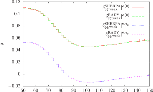
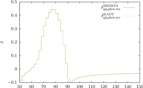
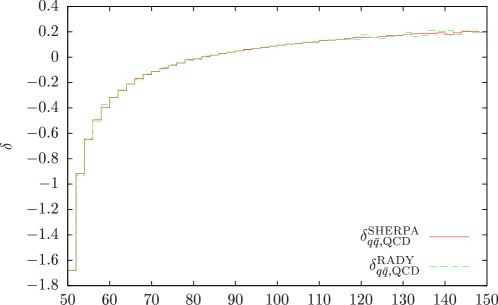
27 THE LHA FOR MONTE CARLO TOOLS AND ONE-LOOP PROGRAMS: AN APPLICATION USING BlackHat AND Rocket WITH MadFKS

27.1 Introduction

In the last few years much progress has been made in the computation of next-to-leading (NLO) computations [515]. The high energy physics community has reached the point where many of these calculations can be done almost automatically. In many cases two separate codes are needed for a full NLO generator:

• the One-Loop Program (OLP) which calculates the virtual contributions to a process for a given phase-space point,

• the Monte Carlo (MC) tool which takes care of the real emission, the subtraction terms and the phase-space integration.

Only together, the OLP and MC codes can provide total cross sections and distributions at NLO accuracy.

To facilitate the usage of the OLP together with any MC an interface has been proposed during the Les Houches 2009 workshop [24]. In this contribution we show how this interface has been implemented in the MC code MadFKS [516] and the OLP codes BlackHat [104, 105, 106] and Rocket [111, 26, 126] and how it works in practice in the process $e^{+}e^{-}\to n$ jets with $n=2,3,4$.

27.2 Code snippets

Before discussing the details of the interfaces between MadFKS and BlackHat or Rocket, we shortly remind the reader about the proposed LHA interface. More details about the proposal can be found in [24].

27.2.1 The proposal for the interface in short

The first stage of using a OLP code with a MC code is the agreement over the process and all related settings via a so-called order file, written by the MC and read by the OLP, and the corresponding contract file written by the OLP. These settings include all relevant input parameters, possible approximations (e.g. the leading color approximation) and the treatment of the helicity (e.g. sum of or Monte Carlo over helicities). Because this initialization stage does not involve linking the codes together, it will not be discussed further in this note.

After an agreement has been established on the process that will be computed and all relevant settings and parameters the actual run can start. During run-time there are two more stages in the interface. First the OLP will read the contract file and will set the corresponding input parameters. The momenta and dynamical input parameters (such as the renormalization scale and the strong coupling) are passed from the MC code to the OLP for each phase-space point. The OLP performs the calculation of the renormalized virtual matrix element squared and returns the value for the loop corrections as an expansion in $1/\epsilon$. The MC code then combines this result with the real radiation term and performs the phase-space integration.

In practice, when interfacing MadFKS with either BlackHat or Rocket, a library from the OLP code has been created. This library can then be linked to MadFKS and all information between the OLP code and the MC code can be passed by subroutine calls. Notice that the various codes can be written in different languages, for instance BlackHat is written in C++, Rocket in Fortran95 and MadFKS in Fortran77. We start by first describing the interface between Rocket and MadFKS, which is slightly simpler.

27.2.2 Linking Rocket to MadFKS

Because Fortran95 and Fortran77 are quite similar, no special treatment is needed if a compiler is used that is compatible with both languages, such as gfortran. Notice however that because Fortran77 cannot handle modules, subroutines that need to be called by MadFKS  have not been placed inside a module in the Rocket.

In practice we use the following function call in MadFKS to start-up the process:

 call OLP_start(filename,status)

where filename is the name of the agreed-upon contract file and status is set to ‘1’ by the OLP for a correctly initialized contract file. During run-time the following call is used to pass the information about the phase-space point:

 call Rocket_EvalSubproc(procnum,nexternal,p,hel,mu,alphaS,virt_wgts).

According to the proposed Les Houches Accord, procnum is the number that Rocket gives to the process in the contract file, p is a linear array containing four-momenta and masses of the external particles, mu is the renormalization scale, alphaS is the strong coupling evaluated at mu, and virt_wgts  is a four-component array with, in order, the double pole, single pole, finite part of the virtual matrix element squared and the Born squared for the given phase-space point p. We also include the number of the external particles and their helicities in the call, even though this is not (yet) part of the LHA proposal. The helicities are passed from MadFKS to Rocket by the array hel to facilitate a Monte Carlo over the helicities. The number of external particles is passed by nexternal. Although not strictly necessary because this information can be deduced from the process in the contract file, in practice it is simpler for the declaration of the arrays p and hel to have their sizes available as an argument of the subroutine.

In Fig. 77 we show an example of a contract file that is used for one of the subprocesses contributing to the NLO corrections to $e^{-}e^{+}\to 3$ jets. All the necessary parameters are specified in this contract, in the right column a brief explanation of the parameters is given. The string “OK” means that the running option or parameter is allowed, but other than that this information is for the user and is not used by the OLP or the MC. A string “ERROR” would indicate that the option/parameter required through the order file by the MC is not allowed and the initialization stage of the OLP will fail.

            # contract produced by Rocket from ’order.file’

            MatrixElementSquareType C_SUMMED  |  OK note: color summed
            IRregularization DR               |  OK note: DR scheme
            CorrectionType QCD                |  OK note: NLO QCD corrections
            Only_Z false                      |  OK note: photon contribution included
            Only_Photon false                 |  OK note: Z contribution included
            Nf_light 5                        |  OK note: nr of light flavours
            IAlpha_EM_MZ 128.802              |  OK note: Inverse of em coupling
            Alpha_S_MZ  0.1190000             |  OK note: Strong coupling
            SinThW2 0.23                      |  OK note: Sin(Th_W)^2
            Mass_Z 91.188                     |  OK note: Z mass
            Width_Z 2.43000                   |  OK note: Z Width
            Color treatment Full Color        |  OK note: Full Color
            Virtual Full NLO                  |  OK note: Full NLO

            2 -> 3 11 -11 1 -1 21             | 1 4 note: process  4

Figure 77: An example of a contract file used with Rocket in $e^{-}e^{+}\to d\bar{d}g$ production.

27.2.3 Linking BlackHat to MadFKS

When linking a C++ code to a Fortran code there are a couple of issues that should be taken into account.

• First, in Fortran arguments of the subroutines are passed by reference, which should be reflected in the C++ code.

• Multi-dimensional arrays are build in different orders in C++ and Fortran. In particular, this means that in Fortran one can define a two-dimensional array of the momenta of a phase-space point as

    real*8 p(0:4, nexternal)
  

  while in C++ this should be

    double p[nexternal][4]
  

  to get the one-dimensional array in the layout prescribed by the LHA proposal.

• Because Fortran compilers add (multiple) leading and/or trailing underscores to variable names, these need to be added in the C++ libraries. The number of underscores depends on the compiler. Also, Fortran is case insensitive, therefore the names of the subroutines in the OLP code that the MC calls, should be in capitals or completely without capitals, again depending on the fortran compiler. In our case, two trailing underscores and subroutine names in lower case letters are needed.

• Furthermore, strings have to end with a null character in C, which means that this character has to be added when passing the string of the location of the contract file from a Fortran Monte Carlo code to a C++ OLP code.

In practice, this means that during the start-up phase the following calls are used in the MadFKS and BlackHat codes, respectively:

  call OLP_Start(filename//Char(0),status)

and

extern "C" {
   void olp_start__(const char* filename,int& status);
}

During runtime

  call OLP_EvalSubprocess(procnum,p,mu,alphaS,alphaEW,virt_wgts)

and

extern "C" {
   void olp_evalsubprocess__(int& Label,double* p,double& mu,
                    double& alpha_s,double& alpha_ew,double* result);
}

are the call and interface of the subroutine that are used to pass the momenta and all relevant information from MadFKS to BlackHat which returns the virtual matrix element squared. The extern "C" is needed in the C++ code to prevent the symbol names to be mangled by the C++ compiler. It is to be noted that the parameters have to be passed by reference.

27.3 Sample results

As a proof of concept we show here some selected results for NLO predictions to electron–positron collisions to 2, 3 and 4 jets at $\sqrt{\hat{s}}=M_{Z}$ and with the renormalization and factorization scales also equal to the $Z$ boson mass. To define jets we use the $k_{t}$-algorithm and recombine momenta according to the $E$-scheme, i.e. we add up the particles four-momenta.

Figure 78: Inclusive $\cos\theta$ for 2 jet production and Thurst distribution for 3 jet production at LO (blue dashed) and NLO (red solid) using MadFKS and Rocket.

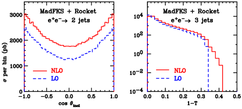
In Fig. 78 results for Rocket linked to MadFKS are plotted. On the left hand side are the LO and NLO predictions shown for the inclusive $\cos\theta$ distribution in 2 jets production. This distribution is defined as the cosine of the angle between the incoming electron direction and all of the final state jets, defined according to the Durham jet algorithm. On the right hand side are the fixed LO and NLO predictions shown of (one minus) the thrust distributions, which starts from Born-level 3 parton events and is therefore shown for $3$-jet events.

Figure 79: $C$ parameter for 3 jet production and $D$ parameter for 4 jet production at LO (blue dashed) and NLO (red solid) using MadFKS and BlackHat.

In Fig. 79 we show two distributions calculated by linking BlackHat code to the MadFKS MC program. In the plot on the left hand side, the $C$ parameter is shown in $e^{+}e^{-}\to 3$ jets at LO and NLO, and in the plot of the right hand side the $D$ parameter in $e^{+}e^{-}\to 4$ jets. [517, 518]

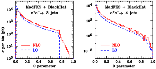
27.4 Conclusions

In this contribution we have shown how the proposed LHA interface between Monte Carlo tools and one-loop programs works in practice between BlackHat or Rocket together with MadFKS. The proposal works well even if the codes are written in different languages. We do not expect that linking other OLP or MC codes using the LHA interface will lead to any further difficulties.

27.5 Acknowledgments

We would like to thank the other members of the BlackHat, MadFKS and Rocket collaborations for their contributions to the development of these codes.

References

- [1] J. M. Campbell, J. W. Huston, and W. J. Stirling, Rept. Prog. Phys. 70 (2007) 89, [hep-ph/0611148].
- [2] C. Buttar et. al., hep-ph/0604120.
- [3] Z. The NLO multileg working group (Bern and others), published in Les Houches 2007, Physics at TeV colliders (2008) 1–120, [arXiv:0803.0494 [hep-ph]].
- [4] S. Dittmaier, S. Kallweit, and P. Uwer, Phys. Rev. Lett. 100 (2008) 062003, [0710.1577].
- [5] S. Dittmaier, S. Kallweit, and P. Uwer, Nucl. Phys. B826 (2010) 18–70, [0908.4124].
- [6] J. M. Campbell, R. K. Ellis, and G. Zanderighi, JHEP 12 (2007) 056, [arXiv:0710.1832 [hep-ph]].
- [7] T. Binoth, T. Gleisberg, S. Karg, N. Kauer, and G. Sanguinetti, Phys. Lett. B683 (2010) 154–159, [0911.3181].
- [8] J. M. Campbell, R. K. Ellis, and G. Zanderighi, JHEP 10 (2006) 028, [hep-ph/0608194].
- [9] M. Ciccolini, A. Denner, and S. Dittmaier, Phys. Rev. Lett. 99 (2007) 161803, [0707.0381].
- [10] M. Ciccolini, A. Denner, and S. Dittmaier, Phys. Rev. D77 (2008) 013002, [0710.4749].
- [11] A. Lazopoulos, K. Melnikov, and F. Petriello, Phys. Rev. D76 (2007) 014001, [hep-ph/0703273].
- [12] V. Hankele and D. Zeppenfeld, Phys. Lett. B661 (2008) 103–108, [0712.3544].
- [13] T. Binoth, G. Ossola, C. G. Papadopoulos, and R. Pittau, JHEP 06 (2008) 082, [0804.0350].
- [14] A. Bredenstein, A. Denner, S. Dittmaier, and S. Pozzorini, Phys. Rev. Lett. 103 (2009) 012002, [arXiv:0905.0110 [hep-ph]].
- [15] A. Bredenstein, A. Denner, S. Dittmaier, and S. Pozzorini, 1001.4006.
- [16] G. Bevilacqua, M. Czakon, C. G. Papadopoulos, R. Pittau, and M. Worek, JHEP 09 (2009) 109, [0907.4723].
- [17] C. F. Berger et. al., Phys. Rev. D80 (2009) 074036, [0907.1984].
- [18] R. K. Ellis, K. Melnikov, and G. Zanderighi, JHEP 04 (2009) 077, [0901.4101].
- [19] G. Bevilacqua, M. Czakon, C. G. Papadopoulos, and M. Worek, 1002.4009.
- [20] B. Jager, C. Oleari, and D. Zeppenfeld, JHEP 07 (2006) 015, [hep-ph/0603177].
- [21] B. Jager, C. Oleari, and D. Zeppenfeld, Phys. Rev. D73 (2006) 113006, [hep-ph/0604200].
- [22] G. Bozzi, B. Jager, C. Oleari, and D. Zeppenfeld, Phys. Rev. D75 (2007) 073004, [hep-ph/0701105].
- [23] T. Binoth et. al., 1001.4905.
- [24] T. Binoth et. al., 1001.1307.
- [25] H.-L. Lai et. al., 0910.4183.
- [26] R. Keith Ellis, K. Melnikov, and G. Zanderighi, Phys. Rev. D80 (2009) 094002, [0906.1445].
- [27] P. M. Nadolsky et. al., Phys. Rev. D78 (2008) 013004, [0802.0007].
- [28] J. Huston, 1001.2581.
- [29] D. C. Dunbar, Nucl. Phys. Proc. Suppl. 183 (2008) 122–136.
- [30] R. K. Ellis, W. T. Giele, and G. Zanderighi, Phys. Rev. D72 (2005) 054018, [hep-ph/0506196].
- [31] S. D. Badger and E. W. N. Glover, Nucl. Phys. Proc. Suppl. 160 (2006) 71–75, [hep-ph/0607139].
- [32] C. F. Berger, V. Del Duca, and L. J. Dixon, Phys. Rev. D74 (2006) 094021, [hep-ph/0608180].
- [33] S. D. Badger, E. W. N. Glover, and K. Risager, JHEP 07 (2007) 066, [0704.3914].
- [34] E. W. N. Glover, P. Mastrolia, and C. Williams, JHEP 08 (2008) 017, [0804.4149].
- [35] L. J. Dixon and Y. Sofianatos, JHEP 08 (2009) 058, [0906.0008].
- [36] S. Badger, E. W. N. Glover, P. Mastrolia, and C. Williams, 0909.4475.
- [37] S. Badger, J. M. Campbell, R. K. Ellis, and C. Williams, 0910.4481.
- [38] Z. Bern, L. J. Dixon, D. C. Dunbar, and D. A. Kosower, Nucl. Phys. B425 (1994) 217–260, [hep-ph/9403226].
- [39] Z. Bern, L. J. Dixon, D. C. Dunbar, and D. A. Kosower, Nucl. Phys. B435 (1995) 59–101, [hep-ph/9409265].
- [40] R. Britto and B. Feng, Phys. Rev. D75 (2007) 105006, [hep-ph/0612089].
- [41] R. Britto and B. Feng, JHEP 02 (2008) 095, [0711.4284].
- [42] R. Britto, B. Feng, and P. Mastrolia, Phys. Rev. D78 (2008) 025031, [0803.1989].
- [43] B. Feng and G. Yang, Nucl. Phys. B811 (2009) 305–352, [0806.4016].
- [44] R. Britto, B. Feng, and G. Yang, JHEP 09 (2008) 089, [0803.3147].
- [45] F. Cachazo, P. Svrcek, and E. Witten, JHEP 09 (2004) 006, [hep-th/0403047].
- [46] G. Georgiou, E. W. N. Glover, and V. V. Khoze, JHEP 07 (2004) 048, [hep-th/0407027].
- [47] L. J. Dixon, E. W. N. Glover, and V. V. Khoze, JHEP 12 (2004) 015, [hep-th/0411092].
- [48] Z. Bern, D. Forde, D. A. Kosower, and P. Mastrolia, Phys. Rev. D72 (2005) 025006, [hep-ph/0412167].
- [49] S. D. Badger, E. W. N. Glover, and V. V. Khoze, JHEP 03 (2005) 023, [hep-th/0412275].
- [50] C. Schwinn and S. Weinzierl, JHEP 05 (2005) 006, [hep-th/0503015].
- [51] K. J. Ozeren and W. J. Stirling, JHEP 11 (2005) 016, [hep-th/0509063].
- [52] R. Boels and C. Schwinn, Phys. Lett. B662 (2008) 80–86, [0712.3409].
- [53] C. Schwinn, Phys. Rev. D78 (2008) 085030, [0809.1442].
- [54] R. Britto, F. Cachazo, and B. Feng, Nucl. Phys. B715 (2005) 499–522, [hep-th/0412308].
- [55] R. Britto, F. Cachazo, B. Feng, and E. Witten, Phys. Rev. Lett. 94 (2005) 181602, [hep-th/0501052].
- [56] M.-x. Luo and C.-k. Wen, JHEP 03 (2005) 004, [hep-th/0501121].
- [57] M.-x. Luo and C.-k. Wen, Phys. Rev. D71 (2005) 091501, [hep-th/0502009].
- [58] J. Bedford, A. Brandhuber, B. J. Spence, and G. Travaglini, Nucl. Phys. B721 (2005) 98–110, [hep-th/0502146].
- [59] F. Cachazo and P. Svrcek, hep-th/0502160.
- [60] R. Britto, B. Feng, R. Roiban, M. Spradlin, and A. Volovich, Phys. Rev. D71 (2005) 105017, [hep-th/0503198].
- [61] S. D. Badger, E. W. N. Glover, V. V. Khoze, and P. Svrcek, JHEP 07 (2005) 025, [hep-th/0504159].
- [62] S. D. Badger, E. W. N. Glover, and V. V. Khoze, JHEP 01 (2006) 066, [hep-th/0507161].
- [63] D. Forde and D. A. Kosower, Phys. Rev. D73 (2006) 065007, [hep-th/0507292].
- [64] P. Ferrario, G. Rodrigo, and P. Talavera, Phys. Rev. Lett. 96 (2006) 182001, [hep-th/0602043].
- [65] K. J. Ozeren and W. J. Stirling, Eur. Phys. J. C48 (2006) 159–168, [hep-ph/0603071].
- [66] C. Schwinn and S. Weinzierl, JHEP 04 (2007) 072, [hep-ph/0703021].
- [67] N. Arkani-Hamed and J. Kaplan, JHEP 04 (2008) 076, [0801.2385].
- [68] A. Brandhuber, P. Heslop, and G. Travaglini, Phys. Rev. D78 (2008) 125005, [0807.4097].
- [69] C. Cheung, 0808.0504.
- [70] J. M. Drummond and J. M. Henn, JHEP 04 (2009) 018, [0808.2475].
- [71] C. Quigley and M. Rozali, JHEP 03 (2006) 004, [hep-ph/0510148].
- [72] C. Cheung and D. O’Connell, JHEP 07 (2009) 075, [0902.0981].
- [73] R. Boels, 0908.0738.
- [74] T. Dennen, Y.-t. Huang, and W. Siegel, 0910.2688.
- [75] P. Mastrolia, Phys. Lett. B678 (2009) 246–249, [0905.2909].
- [76] P. Mastrolia, 0906.3789.
- [77] Z. Bern, L. J. Dixon, and D. A. Kosower, Nucl. Phys. B513 (1998) 3–86, [hep-ph/9708239].
- [78] R. Britto, F. Cachazo, and B. Feng, Nucl. Phys. B725 (2005) 275–305, [hep-th/0412103].
- [79] D. Forde, Phys. Rev. D75 (2007) 125019, [0704.1835].
- [80] W. B. Kilgore, 0711.5015.
- [81] N. E. J. Bjerrum-Bohr, D. C. Dunbar, and W. B. Perkins, JHEP 04 (2008) 038, [0709.2086].
- [82] S. D. Badger, JHEP 01 (2009) 049, [0806.4600].
- [83] Z. Bern and A. G. Morgan, Nucl. Phys. B467 (1996) 479–509, [hep-ph/9511336].
- [84] W. T. Giele, Z. Kunszt, and K. Melnikov, JHEP 04 (2008) 049, [0801.2237].
- [85] R. K. Ellis, W. T. Giele, Z. Kunszt, and K. Melnikov, Nucl. Phys. B822 (2009) 270–282, [0806.3467].
- [86] Z. Bern, L. J. Dixon, and D. A. Kosower, Phys. Rev. D71 (2005) 105013, [hep-th/0501240].
- [87] C. F. Berger, Z. Bern, L. J. Dixon, D. Forde, and D. A. Kosower, Phys. Rev. D74 (2006) 036009, [hep-ph/0604195].
- [88] C. F. Berger, Z. Bern, L. J. Dixon, D. Forde, and D. A. Kosower, Phys. Rev. D75 (2007) 016006, [hep-ph/0607014].
- [89] S. D. Badger, Nucl. Phys. Proc. Suppl. 183 (2008) 220–225, [0807.1245].
- [90] R. Britto and B. Feng, Phys. Lett. B681 (2009) 376–381, [0904.2766].
- [91] G. Ossola, C. G. Papadopoulos, and R. Pittau, Nucl. Phys. B763 (2007) 147–169, [hep-ph/0609007].
- [92] E. W. Nigel Glover and C. Williams, JHEP 12 (2008) 067, [0810.2964].
- [93] S. Catani, T. Gleisberg, F. Krauss, G. Rodrigo, and J.-C. Winter, JHEP 09 (2008) 065, [0804.3170].
- [94] Z. Bern, L. J. Dixon, and D. A. Kosower, Nucl. Phys. B412 (1994) 751–816, [hep-ph/9306240].
- [95] A. Denner, U. Nierste, and R. Scharf, Nucl. Phys. B367 (1991) 637–656.
- [96] A. van Hameren, J. Vollinga, and S. Weinzierl, Eur. Phys. J. C41 (2005) 361–375, [hep-ph/0502165].
- [97] R. K. Ellis and G. Zanderighi, JHEP 02 (2008) 002, [0712.1851].
- [98] S. Badger, N. E. J. Bjerrum-Bohr, and P. Vanhove, JHEP 02 (2009) 038, [0811.3405].
- [99] A. Denner and S. Dittmaier, Nucl. Phys. Proc. Suppl. 157 (2006) 53–57, [hep-ph/0601085].
- [100] A. Denner and S. Dittmaier, Nucl. Phys. B734 (2006) 62–115, [hep-ph/0509141].
- [101] A. Denner and S. Dittmaier, Nucl. Phys. B658 (2003) 175–202, [hep-ph/0212259].
- [102] T. Binoth, J. P. Guillet, G. Heinrich, E. Pilon, and T. Reiter, Comput. Phys. Commun. 180 (2009) 2317–2330, [0810.0992].
- [103] G. Ossola, C. G. Papadopoulos, and R. Pittau, JHEP 03 (2008) 042, [0711.3596].
- [104] C. F. Berger, Z. Bern, L. J. Dixon, D. Forde, and D. A. Kosower, Nucl. Phys. Proc. Suppl. 160 (2006) 261–270, [hep-ph/0610089].
- [105] C. F. Berger et. al., Phys. Rev. D78 (2008) 036003, [0803.4180].
- [106] C. F. Berger et. al., Nucl. Phys. Proc. Suppl. 183 (2008) 313–319, [0807.3705].
- [107] R. K. Ellis, W. T. Giele, and Z. Kunszt, JHEP 03 (2008) 003, [0708.2398].
- [108] R. K. Ellis, W. T. Giele, and Z. Kunszt, PoS RADCOR2007 (2007) 020, [0802.4227].
- [109] W. T. Giele and G. Zanderighi, JHEP 06 (2008) 038, [0805.2152].
- [110] J.-C. Winter and W. T. Giele, 0902.0094.
- [111] K. Melnikov and M. Schulze, JHEP 08 (2009) 049, [0907.3090].
- [112] R. K. Ellis, W. T. Giele, Z. Kunszt, K. Melnikov, and G. Zanderighi, JHEP 01 (2009) 012, [0810.2762].
- [113] A. Lazopoulos, 0812.2998.
- [114] G. Ossola, C. G. Papadopoulos, and R. Pittau, JHEP 05 (2008) 004, [0802.1876].
- [115] G. Ossola, C. G. Papadopoulos, and R. Pittau, PoS RADCOR2007 (2007) 006.
- [116] G. Ossola, C. G. Papadopoulos, and R. Pittau, Nucl. Phys. Proc. Suppl. 183 (2008) 42–47.
- [117] G. Ossola, C. G. Papadopoulos, and R. Pittau, Acta Phys. Polon. B39 (2008) 1685–1694.
- [118] P. Draggiotis, M. V. Garzelli, C. G. Papadopoulos, and R. Pittau, JHEP 04 (2009) 072, [0903.0356].
- [119] M. V. Garzelli, I. Malamos, and R. Pittau, 0910.3130.
- [120] A. van Hameren, C. G. Papadopoulos, and R. Pittau, JHEP 09 (2009) 106, [0903.4665].
- [121] C. F. Berger et. al., 0808.0941.
- [122] C. F. Berger et. al., Phys. Rev. Lett. 102 (2009) 222001, [0902.2760].
- [123] C. F. Berger et. al., 0905.2735.
- [124] C. F. Berger et. al., 0909.4949.
- [125] G. Ossola, C. G. Papadopoulos, and R. Pittau, JHEP 07 (2007) 085, [0704.1271].
- [126] K. Melnikov and G. Zanderighi, 0910.3671.
- [127] A. Lazopoulos, 0911.5241.
- [128] T. Binoth, to appear in the Proc. of the 12th Int. Workshop on Advanced Computing and Analysis Techniques in Physics Research, Erice, Italy, 3 - 7 November 2008 [arXiv:0903.1876 [hep-ph]].
- [129] J. Alwall, S. Hoeche, S. F. Krauss, et. al., Eur. Phys. J. C 53 (2008) 473–500, [arXiv:0706.2569 [hep-ph]].
- [130] A. Cafarella, C. G. Papadopoulos, and M. Worek, Comput. Phys. Commun. 180 (2009) 1941–1955, [0710.2427].
- [131] T. Gleisberg, S. Hoeche, F. Krauss, et. al., JHEP 0402 (2004) 056, [arXiv:hep-ph/0311263].
- [132] T. Gleisberg, S. Hoeche, F. Krauss, et. al., JHEP 0902 (2009) 007, [arXiv:0811.4622 [hep-ph]].
- [133] G. Passarino and M. J. G. Veltman, Nucl. Phys. B 160 (1979) 151.
- [134] C. F. Berger and D. Forde, arXiv:0912.3534 [hep-ph].
- [135] Z. Bern, L. J. Dixon, and D. A. Kosower, Phys. Rev. Lett. 70 (1993) 2677, [arXiv:hep-ph/9302280].
- [136] Z. Bern, L. J. Dixon, and D. A. Kosower, Nucl. Phys. B 437 (1995) 259, [arXiv:hep-ph/9409393].
- [137] T. Binoth, J. P. Guillet, and G. Heinrich, JHEP 02 (2007) 013, [hep-ph/0609054].
- [138] J. A. M. Vermaseren, arXiv:math-ph/0010025.
- [139] J. A. M. Vermaseren, Nucl. Phys. Proc. Suppl. 183 (2008) 19, [arXiv:0806.4080 [hep-ph]].
- [140] D. Y. Bardin and G. Passarino, The standard model in the making: Precision study of the electroweak interactions, Oxford, UK: Clarendon (1999) 685 p.
- [141] A. Denner, G. Weiglein, and S. Dittmaier, Nucl. Phys. B 440 (1995) 95, [arXiv:hep-ph/9410338].
- [142] A. Denner, S. Dittmaier, and G. Weiglein, Proc. of the Ringberg Workshop “Perspectives for electroweak interactions in collisions”, Ringberg Castle, 5 - 8 February 1995, [arXiv:hep-ph/9505271].
- [143] A. van Hameren, JHEP 0907 (2009) 088, [arXiv:0905.1005 [hep-ph]].
- [144] M. V. G. A. v. H. C. G. P. R. P. G. Bevilacqua, M. Czakon and M. Worek,.
- [145] N. E. Adam et. al., 0803.1154.
- [146] T. Binoth, J. P. Guillet, G. Heinrich, E. Pilon, and C. Schubert, JHEP 10 (2005) 015, [hep-ph/0504267].
- [147] T. Binoth, J. P. Guillet, and G. Heinrich, Nucl. Phys. B572 (2000) 361–386, [hep-ph/9911342].
- [148] T. Hahn and M. Perez-Victoria, Comput. Phys. Commun. 118 (1999) 153–165, [hep-ph/9807565].
- [149] T. Hahn, Comput. Phys. Commun. 140 (2001) 418–431, [hep-ph/0012260].
- [150] G. J. van Oldenborgh and J. A. M. Vermaseren, Z. Phys. C46 (1990) 425–438.
- [151] P. Nogueira, J. Comput. Phys. 105 (1993) 279–289.
- [152] A. Pukhov et. al., hep-ph/9908288.
- [153] N. D. Christensen and C. Duhr, Comput. Phys. Commun. 180 (2009) 1614–1641, [0806.4194].
- [154] G. Cullen, M. Koch-Janusz, and T. Reiter,. in preparation.
- [155] A. Denner, H. Eck, O. Hahn, and J. Kublbeck, Nucl. Phys. B387 (1992) 467–484.
- [156] A. Denner, H. Eck, O. Hahn, and J. Kublbeck, Phys. Lett. B291 (1992) 278–280.
- [157] T. Reiter, 0907.3714.
- [158] M. Ceberio and V. Kreinovich, ACM 38 (March, 2004) 8–15.
- [159] S. Gopalakrishnan and P. Kalla, Proc. of Design, Automation and Test in Europe (DATE ’09) (2009) 1452–1457.
- [160] M. Poletto and V. Sarkar, ACM Transactions on Programming Languages and Systems 21 (September, 1999) 895–913.
- [161] J. A. M. Vermaseren, Comput. Phys. Commun. 83 (1994) 45–58.
- [162] T. Ohl, Comput. Phys. Commun. 90 (1995) 340–354, [hep-ph/9505351].
- [163] R. Lafaye, D. J. Miller, 2, M. Muhlleitner, and S. Moretti, hep-ph/0002238.
- [164] T. Stelzer and W. F. Long, Comput. Phys. Commun. 81 (1994) 357–371, [hep-ph/9401258].
- [165] F. Maltoni and T. Stelzer, JHEP 02 (2003) 027, [hep-ph/0208156].
- [166] R. Frederix, T. Gehrmann, and N. Greiner, JHEP 09 (2008) 122, [0808.2128].
- [167] W. Kilian, T. Ohl, and J. Reuter, 0708.4233.
- [168] S. Catani and M. H. Seymour, Nucl. Phys. B485 (1997) 291–419, [hep-ph/9605323].
- [169] Z. Nagy and Z. Trocsanyi, Phys. Lett. B634 (2006) 498–503, [hep-ph/0511328].
- [170] G. C. Blazey et. al., hep-ex/0005012.
- [171] J. Pumplin et. al., JHEP 07 (2002) 012, [hep-ph/0201195].
- [172] A. Semenov, Comput. Phys. Commun. 180 (2009) 431–454, [0805.0555].
- [173] S. Frixione, P. Nason, and C. Oleari, JHEP 11 (2007) 070, [0709.2092].
- [174] J. M. Campbell and R. K. Ellis,. MCFM v5.6: A Monte Carlo for Femtobarn processes at Hadron Colliders (Manual).
- [175] I. Antcheva et. al., Comput. Phys. Commun. 180 (2009) 2499–2512.
- [176] LHEF 2.0 specification, these proceedings.
- [177] S. Dittmaier, P. Uwer, and S. Weinzierl, Phys. Rev. Lett. 98 (2007) 262002, [hep-ph/0703120].
- [178] S. Dittmaier, P. Uwer, and S. Weinzierl, Eur. Phys. J. C59 (2009) 625–646, [0810.0452].
- [179] http://cern.ch/fpschill/LesHouchesNLOTrees.
- [180] S. Catani,. presented at the Workshop : High Precision for Hard Processes at the LHC, Sept. 2006, Zurich, Switzerland.
- [181] T. Gleisberg, Ph.D. Thesis, University of Dresden (2007).
- [182] D. E. Soper, Phys. Rev. Lett. 81 (1998) 2638–2641, [hep-ph/9804454].
- [183] M. Kramer and D. E. Soper, Phys. Rev. D66 (2002) 054017, [hep-ph/0204113].
- [184] T. Kleinschmidt, DESY-THESIS-2007-042 (2007).
- [185] M. Moretti, F. Piccinini, and A. D. Polosa, hep-ph/0802.4171.
- [186] W. Beenakker et. al., Phys. Rev. Lett. 87 (2001) 201805, [hep-ph/0107081].
- [187] W. Beenakker et. al., Nucl. Phys. B653 (2003) 151–203, [hep-ph/0211352].
- [188] S. Dawson, L. H. Orr, L. Reina, and D. Wackeroth, Phys. Rev. D67 (2003) 071503, [hep-ph/0211438].
- [189] S. Dawson, C. Jackson, L. H. Orr, L. Reina, and D. Wackeroth, Phys. Rev. D68 (2003) 034022, [hep-ph/0305087].
- [190] A. Bredenstein, A. Denner, S. Dittmaier, and S. Pozzorini, JHEP 08 (2008) 108, [0807.1248].
- [191] T. Plehn, G. P. Salam, and M. Spannowsky, 0910.5472.
- [192] A. Djouadi, J. Kalinowski, and M. Spira, Comput. Phys. Commun. 108 (1998) 56–74, [hep-ph/9704448].
- [193] A. Kanaki and C. G. Papadopoulos, Comput. Phys. Commun. 132 (2000) 306–315, [hep-ph/0002082].
- [194] C. G. Papadopoulos, Comput. Phys. Commun. 137 (2001) 247–254, [hep-ph/0007335].
- [195] C. G. Papadopoulos and M. Worek, Eur. Phys. J. C50 (2007) 843–856, [hep-ph/0512150].
- [196] M. Czakon, C. G. Papadopoulos, and M. Worek, JHEP 08 (2009) 085, [0905.0883].
- [197] D. Stump et. al., JHEP 10 (2003) 046, [hep-ph/0303013].
- [198] S. Catani, Y. L. Dokshitzer, and B. R. Webber, Phys. Lett. B285 (1992) 291–299.
- [199] S. Catani, Y. L. Dokshitzer, M. H. Seymour, and B. R. Webber, Nucl. Phys. B406 (1993) 187–224.
- [200] S. D. Ellis and D. E. Soper, Phys. Rev. D48 (1993) 3160–3166, [hep-ph/9305266].
- [201] S. Catani, S. Dittmaier, M. H. Seymour, and Z. Trocsanyi, Nucl. Phys. B627 (2002) 189–265, [hep-ph/0201036].
- [202] B. P. Kersevan and E. Richter-Was, Eur. Phys. J. C25 (2002) 379–389, [hep-ph/0203148].
- [203] B. P. Kersevan and E. Richter-Was, Comput. Phys. Commun. 149 (2003) 142–194, [hep-ph/0201302].
- [204] J. Cammin and M. Schumacher, ATL-PHYS-2003-024.
- [205] G. Aad et. al.,, The ATLAS Collaboration 0901.0512.
- [206] Drollinger, V. and Müller, T. and Denegri, D., hep-ph/0111312.
- [207] S. Cucciarelli et. al., CMS Note 2006/119.
- [208] D. Benedetti et. al., J. Phys. G34 (2007) N221–N250.
- [209] G. L. Bayatian et. al.,, CMS Collaboration J. Phys. G34 (2007) 995–1579.
- [210] A. Lazopoulos, T. McElmurry, K. Melnikov, and F. Petriello, Phys. Lett. B666 (2008) 62–65, [0804.2220].
- [211] Tevatron Electroweak Working Group Collaboration 0803.1683.
- [212] Z. Bern, L. J. Dixon, and V. A. Smirnov, Phys. Rev. D72 (2005) 085001, [hep-th/0505205].
- [213] M. Dasgupta and G. P. Salam, J. Phys. G30 (2004) R143, [hep-ph/0312283].
- [214] E. Gardi, hep-ph/0606080.
- [215] T. Becher and M. Neubert, Phys. Rev. Lett. 102 (2009) 162001, [0901.0722].
- [216] E. Gardi and L. Magnea, JHEP 03 (2009) 079, [0901.1091].
- [217] T. Becher and M. Neubert, JHEP 06 (2009) 081, [0903.1126].
- [218] E. Gardi and L. Magnea, Nuovo Cimento 32C (2009) 137, [0908.3273].
- [219] L. Magnea and G. Sterman, Phys. Rev. D42 (1990) 4222–4227.
- [220] L. Magnea, Nucl. Phys. B593 (2001) 269–288, [hep-ph/0006255].
- [221] G. P. Korchemsky and A. V. Radyushkin, Phys. Lett. B171 (1986) 459–467.
- [222] S. M. Aybat, L. J. Dixon, and G. Sterman, Phys. Rev. Lett. 97 (2006) 072001, [hep-ph/0606254].
- [223] S. M. Aybat, L. J. Dixon, and G. Sterman, Phys. Rev. D74 (2006) 074004, [hep-ph/0607309].
- [224] L. J. Dixon, Phys. Rev. D79 (2009) 091501, [0901.3414].
- [225] G. Sterman and M. E. Tejeda-Yeomans, Phys. Lett. B552 (2003) 48–56, [hep-ph/0210130].
- [226] L. J. Dixon, L. Magnea, and G. Sterman, JHEP 08 (2008) 022, [0805.3515].
- [227] S. Catani, B. R. Webber, and G. Marchesini, Nucl. Phys. B349 (1991) 635–654.
- [228] E. Gardi and R. G. Roberts, Nucl. Phys. B653 (2003) 227–255, [hep-ph/0210429].
- [229] E. Gardi and G. Grunberg, Nucl. Phys. B794 (2008) 61–137, [0709.2877].
- [230] T. Becher and M. Neubert, Phys. Rev. D79 (2009) 125004, [0904.1021].
- [231] A. Ferroglia, M. Neubert, B. D. Pecjak, and L. L. Yang, Phys. Rev. Lett. 103 (2009) 201601, [0907.4791].
- [232] A. Ferroglia, M. Neubert, B. D. Pecjak, and L. L. Yang, JHEP 11 (2009) 062, [0908.3676].
- [233] A. Armoni, JHEP 11 (2006) 009, [hep-th/0608026].
- [234] L. Dixon, E. Gardi, and L. Magnea, JHEP 02 (2010) 081, [0910.3653].
- [235] A. Gehrmann-De Ridder, T. Gehrmann, E. W. N. Glover, and G. Heinrich, JHEP 12 (2007) 094, [0711.4711].
- [236] A. Gehrmann-De Ridder, T. Gehrmann, E. W. N. Glover, and G. Heinrich, Phys. Rev. Lett. 99 (2007) 132002, [0707.1285].
- [237] A. Gehrmann-De Ridder, T. Gehrmann, E. W. N. Glover, and G. Heinrich, Phys. Rev. Lett. 100 (2008) 172001, [0802.0813].
- [238] A. Gehrmann-De Ridder, T. Gehrmann, E. W. N. Glover, and G. Heinrich, JHEP 05 (2009) 106, [0903.4658].
- [239] S. Weinzierl, Phys. Rev. Lett. 101 (2008) 162001, [0807.3241].
- [240] S. Weinzierl, JHEP 06 (2009) 041, [0904.1077].
- [241] S. Weinzierl, Phys. Rev. D80 (2009) 094018, [0909.5056].
- [242] L. W. Garland, T. Gehrmann, E. W. N. Glover, A. Koukoutsakis, and E. Remiddi, Nucl. Phys. B642 (2002) 227–262, [hep-ph/0206067].
- [243] S. Moch, P. Uwer, and S. Weinzierl, Phys. Rev. D66 (2002) 114001, [hep-ph/0207043].
- [244] Z. Bern, L. Dixon, D. A. Kosower, and S. Weinzierl, Nucl. Phys. B489 (1997) 3–23, [hep-ph/9610370].
- [245] J. M. Campbell, E. W. N. Glover, and D. J. Miller, Phys. Lett. B409 (1997) 503–508, [hep-ph/9706297].
- [246] E. W. N. Glover and D. J. Miller, Phys. Lett. B396 (1997) 257–263, [hep-ph/9609474].
- [247] F. A. Berends, W. T. Giele, and H. Kuijf, Nucl. Phys. B321 (1989) 39.
- [248] K. Hagiwara and D. Zeppenfeld, Nucl. Phys. B313 (1989) 560.
- [249] Z. Nagy and Z. Trocsanyi, Phys. Rev. D59 (1999) 014020, [hep-ph/9806317].
- [250] T. Gehrmann and E. Remiddi, Nucl. Phys. B580 (2000) 485–518, [hep-ph/9912329].
- [251] T. Gehrmann and E. Remiddi, Nucl. Phys. B601 (2001) 248–286, [hep-ph/0008287].
- [252] T. Gehrmann and E. Remiddi, Nucl. Phys. B601 (2001) 287–317, [hep-ph/0101124].
- [253] S. Moch, P. Uwer, and S. Weinzierl, J. Math. Phys. 43 (2002) 3363–3386, [hep-ph/0110083].
- [254] S. Weinzierl, Comput. Phys. Commun. 145 (2002) 357–370, [math-ph/0201011].
- [255] S. Moch and P. Uwer, Comput. Phys. Commun. 174 (2006) 759–770, [math-ph/0508008].
- [256] T. Gehrmann and E. Remiddi, Comput. Phys. Commun. 141 (2001) 296–312, [hep-ph/0107173].
- [257] T. Gehrmann and E. Remiddi, Comput. Phys. Commun. 144 (2002) 200–223, [hep-ph/0111255].
- [258] J. Vollinga and S. Weinzierl, Comput. Phys. Commun. 167 (2005) 177, [hep-ph/0410259].
- [259] A. Gehrmann-De Ridder, T. Gehrmann, and E. W. N. Glover, JHEP 09 (2005) 056, [hep-ph/0505111].
- [260] A. Gehrmann-De Ridder, T. Gehrmann, E. W. N. Glover, and G. Heinrich, JHEP 11 (2007) 058, [arXiv:0710.0346 [hep-ph]].
- [261] S. Weinzierl, Phys. Rev. D74 (2006) 014020, [hep-ph/0606008].
- [262] S. Weinzierl, JHEP 07 (2009) 009, [0904.1145].
- [263] S. Weinzierl and D. A. Kosower, Phys. Rev. D60 (1999) 054028, [hep-ph/9901277].
- [264] C. W. Bauer and B. O. Lange, 0905.4739.
- [265] G. P. Salam and G. Soyez, JHEP 05 (2007) 086, [0704.0292].
- [266] S. Catani and M. H. Seymour, Nucl. Phys. Erratum-ibid. B510 (1998) 503–504.
- [267] T. Gleisberg and F. Krauss, Eur. Phys. J. C53 (2008) 501–523, [0709.2881].
- [268] T. Gleisberg et. al., http://www.sherpa-mc.de.
- [269] S. Höche, F. Krauss, S. Schumann, and F. Siegert, JHEP 05 (2009) 053, [0903.1219].
- [270] S. Höche, S. Schumann, and F. Siegert, 0912.3501.
- [271] T. Carli, T. Gehrmann, and S. Höche, 0912.3715.
- [272] T. Gleisberg and S. Höche, JHEP 12 (2008) 039, [0808.3674].
- [273] S. Catani, F. Krauss, R. Kuhn, and B. R. Webber, JHEP 11 (2001) 063, [hep-ph/0109231].
- [274] A. Schälicke and F. Krauss, JHEP 07 (2005) 018, [hep-ph/0503281].
- [275] V. M. Abazov et. al.,, D0 Collaboration Phys. Rev. Lett. 103 (2009) 092001, [0903.0850].
- [276] T. Aaltonen et. al.,, CDF Collaboration Phys. Rev. Lett. 103 (2009) 092002, [0903.0885].
- [277] J. M. Campbell, R. Frederix, F. Maltoni, and F. Tramontano, Phys. Rev. Lett. 102 (2009) 182003, [0903.0005].
- [278] E. E. Boos, V. E. Bunichev, L. V. Dudko, V. I. Savrin, and A. V. Sherstnev, Phys. Atom. Nucl. 69 (2006) 1317–1329.
- [279] E. Boos et. al.,, CompHEP Collaboration Nucl. Instrum. Meth. A534 (2004) 250–259, [hep-ph/0403113].
- [280] T. Sjostrand, S. Mrenna, and P. Z. Skands, JHEP 05 (2006) 026, [hep-ph/0603175].
- [281] J. M. Campbell, R. Frederix, F. Maltoni, and F. Tramontano, JHEP 10 (2009) 042, [0907.3933].
- [282] F. Campanario, C. Englert, M. Spannowsky, and D. Zeppenfeld, Europhys. Lett. 88 (2009) 11001, [0908.1638].
- [283] S. Dittmaier, S. Kallweit, and P. Uwer, in preparation.
- [284] S. Kallweit, PhD thesis, LMU Munich (2008).
- [285] R. K. Ellis, D. A. Ross, and A. E. Terrano, Nucl. Phys. B178 (1981) 421.
- [286] J. Küblbeck, M. Böhm, and A. Denner, Comput. Phys. Commun. 60 (1990) 165–180.
- [287] S. Dittmaier, Nucl. Phys. B675 (2003) 447–466, [hep-ph/0308246].
- [288] G. ’t Hooft and M. J. G. Veltman, Nucl. Phys. B153 (1979) 365–401.
- [289] W. Beenakker and A. Denner, Nucl. Phys. B338 (1990) 349–370.
- [290] G. J. van Oldenborgh, Comput. Phys. Commun. 66 (1991) 1–15.
- [291] F. A. Berends, R. Pittau, and R. Kleiss, Nucl. Phys. B424 (1994) 308–342, [hep-ph/9404313].
- [292] R. Kleiss and R. Pittau, Comput. Phys. Commun. 83 (1994) 141–146, [hep-ph/9405257].
- [293] Z. Xu, D.-H. Zhang, and L. Chang, Nucl. Phys. B291 (1987) 392.
- [294] G. ’t Hooft and M. J. G. Veltman, Nucl. Phys. B44 (1972) 189–213.
- [295] P. Breitenlohner and D. Maison, Commun. Math. Phys. 52 (1977) 39.
- [296] S. A. Larin, Phys. Lett. B303 (1993) 113–118, [hep-ph/9302240].
- [297] T. L. Trueman, Z. Phys. C69 (1996) 525–536, [hep-ph/9504315].
- [298] B. W. Harris, E. Laenen, L. Phaf, Z. Sullivan, and S. Weinzierl, Phys. Rev. D66 (2002) 054024, [hep-ph/0207055].
- [299] N. Kauer and D. Zeppenfeld, Phys. Rev. D65 (2002) 014021, [hep-ph/0107181].
- [300] F. Krauss, R. Kuhn, and G. Soff, JHEP 02 (2002) 044, [hep-ph/0109036].
- [301] M. Dittmar and H. K. Dreiner, Phys. Rev. D55 (1997) 167–172, [hep-ph/9608317].
- [302] R. W. Brown and K. O. Mikaelian, Phys. Rev. D19 (1979) 922.
- [303] J. Ohnemus, Phys. Rev. D44 (1991) 1403–1414.
- [304] S. Frixione, Nucl. Phys. B410 (1993) 280–324.
- [305] L. J. Dixon, Z. Kunszt, and A. Signer, Nucl. Phys. B531 (1998) 3–23, [hep-ph/9803250].
- [306] L. J. Dixon, Z. Kunszt, and A. Signer, Phys. Rev. D60 (1999) 114037, [hep-ph/9907305].
- [307] J. M. Campbell and R. K. Ellis, Phys. Rev. D60 (1999) 113006, [hep-ph/9905386].
- [308] M. Grazzini, JHEP 01 (2006) 095, [hep-ph/0510337].
- [309] M. Spira, A. Djouadi, D. Graudenz, and P. M. Zerwas, Nucl. Phys. B453 (1995) 17–82, [hep-ph/9504378].
- [310] S. Dawson, Nucl. Phys. B359 (1991) 283–300.
- [311] R. V. Harlander and W. B. Kilgore, Phys. Rev. Lett. 88 (2002) 201801, [hep-ph/0201206].
- [312] C. Anastasiou and K. Melnikov, Nucl. Phys. B646 (2002) 220–256, [hep-ph/0207004].
- [313] V. Ravindran, J. Smith, and W. L. van Neerven, Nucl. Phys. B665 (2003) 325–366, [hep-ph/0302135].
- [314] S. Catani, D. de Florian, and M. Grazzini, JHEP 01 (2002) 015, [hep-ph/0111164].
- [315] G. Davatz, G. Dissertori, M. Dittmar, M. Grazzini, and F. Pauss, JHEP 05 (2004) 009, [hep-ph/0402218].
- [316] C. Anastasiou, K. Melnikov, and F. Petriello, Phys. Rev. Lett. 93 (2004) 262002, [hep-ph/0409088].
- [317] C. Anastasiou, G. Dissertori, and F. Stockli, JHEP 09 (2007) 018, [0707.2373].
- [318] M. Grazzini, JHEP 02 (2008) 043, [0801.3232].
- [319] A. Bredenstein, A. Denner, S. Dittmaier, and M. M. Weber, Phys. Rev. D74 (2006) 013004, [hep-ph/0604011].
- [320] T. Binoth, M. Ciccolini, N. Kauer, and M. Kramer, JHEP 03 (2005) 065, [hep-ph/0503094].
- [321] T. Binoth, M. Ciccolini, N. Kauer, and M. Kramer, JHEP 12 (2006) 046, [hep-ph/0611170].
- [322] G. Chachamis, Acta Phys. Polon. B38 (2007) 3563–3568, [0710.3035].
- [323] G. Chachamis, M. Czakon, and D. Eiras, JHEP 12 (2008) 003, [0802.4028].
- [324] G. Chachamis, M. Czakon, and D. Eiras, 0806.3043.
- [325] M. Caffo, H. Czyz, S. Laporta, and E. Remiddi, Nuovo Cim. A111 (1998) 365–389, [hep-th/9805118].
- [326] R. Boughezal, M. Czakon, and T. Schutzmeier, JHEP 09 (2007) 072, [0707.3090].
- [327] M. Czakon and T. Schutzmeier, JHEP 07 (2008) 001, [0712.2762].
- [328] M. Czakon, A. Mitov, and S. Moch, Phys. Lett. B651 (2007) 147–159, [0705.1975].
- [329] M. Czakon, A. Mitov, and S. Moch, Nucl. Phys. B798 (2008) 210–250, [0707.4139].
- [330] S. Laporta, Int. J. Mod. Phys. A15 (2000) 5087–5159, [hep-ph/0102033].
- [331] V. A. Smirnov, Phys. Lett. B460 (1999) 397–404, [hep-ph/9905323].
- [332] J. B. Tausk, Phys. Lett. B469 (1999) 225–234, [hep-ph/9909506].
- [333] G. Chachamis and M. Czakon, Publication in preparation.
- [334] M. Czakon, Comput. Phys. Commun. 175 (2006) 559–571, [hep-ph/0511200].
- [335] H. R. P. Ferguson and D. H. Bailey, Math. of Comput. 53 (1989) 649.
- [336] M. Czakon, Phys. Lett. B664 (2008) 307–314, [0803.1400].
- [337] P. N. Brown, G. D. Byrne, and A. C. Hindmarsh, SIAM J. Sci. Stat. Comput. (1989) 1038.
- [338] G. Chachamis and M. Czakon, Publication in preparation.
- [339] L. N. Lipatov, Sov. J. Nucl. Phys. 20 (1975) 94–102.
- [340] V. S. Fadin, E. A. Kuraev, and L. N. Lipatov, Phys. Lett. B60 (1975) 50–52.
- [341] E. A. Kuraev, L. N. Lipatov, and V. S. Fadin, Sov. Phys. JETP 44 (1976) 443–450.
- [342] I. I. Balitsky, L. N. Lipatov, and V. S. Fadin,. In *Leningrad 1979, Proceedings, Physics Of Elementary Particles*, Leningrad 1979, 109-149.
- [343] J. R. Andersen, V. Del Duca, F. Maltoni, and W. J. Stirling, JHEP 05 (2001) 048, [hep-ph/0105146].
- [344] J. R. Andersen and W. J. Stirling, JHEP 02 (2003) 018, [hep-ph/0301081].
- [345] J. R. Andersen and C. D. White, Phys. Rev. D78 (2008) 051501, [0802.2858].
- [346] J. R. Andersen, V. Del Duca, and C. D. White, JHEP 02 (2009) 015, [0808.3696].
- [347] J. R. Andersen and J. M. Smillie, JHEP 01 (2010) 039, [0908.2786].
- [348] J. R. Andersen and J. M. Smillie, 0910.5113.
- [349] Y. L. Dokshitzer, V. A. Khoze, and T. Sjostrand, Phys. Lett. B274 (1992) 116–121.
- [350] J. M. Campbell, R. K. Ellis, and D. L. Rainwater, Phys. Rev. D68 (2003) 094021, [hep-ph/0308195].
- [351] G. Corcella et. al., hep-ph/0210213.
- [352] T. Sjostrand, S. Mrenna, and P. Z. Skands, Comput. Phys. Commun. 178 (2008) 852–867, [0710.3820].
- [353] M. L. Mangano, M. Moretti, F. Piccinini, R. Pittau, and A. D. Polosa, JHEP 07 (2003) 001, [hep-ph/0206293].
- [354] C. F. Berger et. al., 0912.4927.
- [355] C. Anastasiou, K. Melnikov, and F. Petriello, Nucl. Phys. B724 (2005) 197–246, [hep-ph/0501130].
- [356] C. Anastasiou, G. Dissertori, M. Grazzini, F. Stockli, and B. R. Webber, JHEP 08 (2009) 099, [0905.3529].
- [357] G. Bernardi et. al.,, Tevatron New Phenomena Higgs Working Group Collaboration 0808.0534.
- [358] CDF Collaboration 0903.4001.
- [359] T. Aaltonen et. al.,, CDF Collaboration Phys. Rev. Lett. 102 (2009) 021802, [0809.3930].
- [360] C. Collaboration,, “Search for production at using of data.” CDF conference note 9500.
- [361] D. Collaboration,, “Search for higgs boson production in dilepton plus missing transverse energy final states with of collisions at .” D0 conference note 5871.
- [362] A. Heister et. al.,, ALEPH Collaboration Eur. Phys. J. C35 (2004) 457–486.
- [363] D. Buskulic et. al.,, ALEPH Collaboration Z. Phys. C73 (1997) 409–420.
- [364] P. D. Acton et. al.,, OPAL Collaboration Z. Phys. C59 (1993) 1–20.
- [365] G. Alexander et. al.,, OPAL Collaboration Z. Phys. C72 (1996) 191–206.
- [366] K. Ackerstaff et. al.,, OPAL Collaboration Z. Phys. C75 (1997) 193–207.
- [367] G. Abbiendi et. al.,, OPAL Collaboration Eur. Phys. J. C16 (2000) 185–210.
- [368] G. Abbiendi et. al.,, OPAL Collaboration Eur. Phys. J. C40 (2005) 287–316.
- [369] M. Acciarri et. al.,, L3 Collaboration Phys. Lett. B371 (1996) 137–148.
- [370] M. Acciarri et. al.,, L3 Collaboration Phys. Lett. B404 (1997) 390–402.
- [371] M. Acciarri et. al.,, L3 Collaboration Phys. Lett. B444 (1998) 569–582.
- [372] P. Achard et. al.,, L3 Collaboration Phys. Lett. B536 (2002) 217–228.
- [373] P. Achard et. al.,, L3 Collaboration Phys. Rept. 399 (2004) 71–174.
- [374] P. Abreu et. al.,, DELPHI Collaboration Phys. Lett. B456 (1999) 322–340.
- [375] J. Abdallah et. al.,, DELPHI Collaboration Eur. Phys. J. C29 (2003) 285–312.
- [376] J. Abdallah et. al.,, DELPHI Collaboration Eur. Phys. J. C37 (2004) 1–23.
- [377] P. A. Movilla Fernandez, O. Biebel, S. Bethke, S. Kluth, and P. Pfeifenschneider,, JADE Collaboration Eur. Phys. J. C1 (1998) 461–478, [hep-ex/9708034].
- [378] C. Pahl, S. Bethke, S. Kluth, J. Schieck, and t. J. collaboration, Eur. Phys. J. C60 (2009) 181–196, [0810.2933].
- [379] S. Catani, L. Trentadue, G. Turnock, and B. R. Webber, Nucl. Phys. B407 (1993) 3–42.
- [380] Z. Kunszt, Phys. Lett. B99 (1981) 429.
- [381] Z. Kunszt and P. Nason,. Z Physics at LEP 1, CERN Yellow Report 89-08, Vol. 1, p. 373.
- [382] G. Dissertori et. al., JHEP 02 (2008) 040, [0712.0327].
- [383] T. Gehrmann, G. Luisoni, and H. Stenzel, Phys. Lett. B664 (2008) 265–273, [0803.0695].
- [384] G. Dissertori et. al., JHEP 08 (2009) 036, [0906.3436].
- [385] A. Denner, S. Dittmaier, T. Gehrmann, and C. Kurz, Phys. Lett. B679 (2009) 219–222, [0906.0372].
- [386] S. Bethke, S. Kluth, C. Pahl, and J. Schieck,, JADE Collaboration Eur. Phys. J. C64 (2009) 351–360, [0810.1389].
- [387] R. A. Davison and B. R. Webber, Eur. Phys. J. C59 (2009) 13–25, [0809.3326].
- [388] T. Becher and M. D. Schwartz, JHEP 07 (2008) 034, [0803.0342].
- [389] T. Gehrmann, M. Jaquier, and G. Luisoni, 0911.2422.
- [390] Y. L. Dokshitzer, G. Marchesini, and B. R. Webber, Nucl. Phys. B469 (1996) 93–142, [hep-ph/9512336].
- [391] Y. L. Dokshitzer and B. R. Webber, Phys. Lett. B404 (1997) 321–327, [hep-ph/9704298].
- [392] Y. L. Dokshitzer, A. Lucenti, G. Marchesini, and G. P. Salam, JHEP 05 (1998) 003, [hep-ph/9802381].
- [393] Y. L. Dokshitzer, G. Marchesini, and G. P. Salam, Eur. Phys. J. direct C1 (1999) 3, [hep-ph/9812487].
- [394] E. Farhi, Phys. Rev. Lett. 39 (1977) 1587–1588.
- [395] L. Clavelli and D. Wyler, Phys. Lett. B103 (1981) 383.
- [396] P. E. L. Rakow and B. R. Webber, Nucl. Phys. B191 (1981) 63.
- [397] G. Parisi, Phys. Lett. B74 (1978) 65.
- [398] J. F. Donoghue, F. E. Low, and S.-Y. Pi, Phys. Rev. D20 (1979) 2759.
- [399] W. J. Stirling, J. Phys. G17 (1991) 1567–1574.
- [400] S. Bethke, Z. Kunszt, D. E. Soper, and W. J. Stirling, Nucl. Phys. B370 (1992) 310–334.
- [401] A. Brandenburg and P. Uwer, Nucl. Phys. B515 (1998) 279–320, [hep-ph/9708350].
- [402] W. Bernreuther, A. Brandenburg, and P. Uwer, Phys. Rev. Lett. 79 (1997) 189–192, [hep-ph/9703305].
- [403] G. Rodrigo, A. Santamaria, and M. S. Bilenky, Phys. Rev. Lett. 79 (1997) 193–196, [hep-ph/9703358].
- [404] P. Nason and C. Oleari, Nucl. Phys. B521 (1998) 237–273, [hep-ph/9709360].
- [405] R. W. L. Jones, M. Ford, G. P. Salam, H. Stenzel, and D. Wicke, JHEP 12 (2003) 007, [hep-ph/0312016].
- [406] T. Sjostrand et. al., Comput. Phys. Commun. 135 (2001) 238–259, [hep-ph/0010017].
- [407] G. Corcella et. al., JHEP 01 (2001) 010, [hep-ph/0011363].
- [408] L. Lonnblad, Comput. Phys. Commun. 71 (1992) 15–31.
- [409] R. Barate et. al.,, ALEPH Collaboration Phys. Rept. 294 (1998) 1–165.
- [410] O. Latunde-Dada, JHEP 11 (2007) 040, [0708.4390].
- [411] O. Latunde-Dada, S. Gieseke, and B. Webber, JHEP 02 (2007) 051, [hep-ph/0612281].
- [412] S. Frixione and B. R. Webber, JHEP 06 (2002) 029, [hep-ph/0204244].
- [413] P. Nason, JHEP 11 (2004) 040, [hep-ph/0409146].
- [414] K. Hamilton, P. Richardson, and J. Tully, JHEP 11 (2009) 038, [0905.3072].
- [415] G. Dissertori et. al., 0910.4283.
- [416] C. J. Pahl, Ph.D. thesis, MPI Munich 2007.
- [417] T. Han, G. Valencia, and S. Willenbrock, Phys. Rev. Lett. 69 (1992) 3274–3277, [hep-ph/9206246].
- [418] M. Spira, Fortsch. Phys. 46 (1998) 203–284, [hep-ph/9705337].
- [419] T. Figy, C. Oleari, and D. Zeppenfeld, Phys. Rev. D68 (2003) 073005, [hep-ph/0306109].
- [420] T. Figy and D. Zeppenfeld, Phys. Lett. B591 (2004) 297–303, [hep-ph/0403297].
- [421] E. L. Berger and J. Campbell, Phys. Rev. D70 (2004) 073011, [hep-ph/0403194].
- [422] P. Nason and C. Oleari, 0911.5299.
- [423] A. D. Martin, R. G. Roberts, W. J. Stirling, and R. S. Thorne, Eur. Phys. J. C39 (2005) 155–161, [hep-ph/0411040].
- [424] J. M. Butterworth, A. R. Davison, M. Rubin, and G. P. Salam, Phys. Rev. Lett. 100 (2008) 242001, [0802.2470].
- [425] P. Aurenche, R. Baier, and M. Fontannaz, Phys. Rev. D42 (1990) 1440–1449.
- [426] H. Baer, J. Ohnemus, and J. F. Owens, Phys. Rev. D42 (1990) 61–71.
- [427] E. W. N. Glover and A. G. Morgan, Z. Phys. C62 (1994) 311–322.
- [428] A. Gehrmann-De Ridder, T. Gehrmann, and E. W. N. Glover, Phys. Lett. B414 (1997) 354–361, [hep-ph/9705305].
- [429] S. Frixione, Phys. Lett. B429 (1998) 369–374, [hep-ph/9801442].
- [430] L. Carminati, ATL-PHYS-2002-004.
- [431] M. Cacciari, G. P. Salam, and G. Soyez, JHEP 04 (2008) 005, [0802.1188].
- [432] Jetphox is available at: http://lappweb.in2p3.fr/lapth/PHOX_FAMILY/main.html.
- [433] P. Aurenche, M. Fontannaz, J.-P. Guillet, E. Pilon, and M. Werlen, Phys. Rev. D73 (2006) 094007, [hep-ph/0602133].
- [434] Z. Belghobsi et. al., Phys. Rev. D79 (2009) 114024, [0903.4834].
- [435] S. Catani, M. Fontannaz, J. P. Guillet, and E. Pilon, JHEP 05 (2002) 028, [hep-ph/0204023].
- [436] J. Pumplin, A. Belyaev, J. Huston, D. Stump, and W. K. Tung, JHEP 02 (2006) 032, [hep-ph/0512167].
- [437] A. D. Martin, W. J. Stirling, R. S. Thorne, and G. Watt, Eur. Phys. J. C64 (2009) 653–680, [0905.3531].
- [438] S. Forte, L. Garrido, J. I. Latorre, and A. Piccione, JHEP 05 (2002) 062, [hep-ph/0204232].
- [439] L. Del Debbio, S. Forte, J. I. Latorre, A. Piccione, and J. Rojo,, NNPDF Collaboration JHEP 03 (2005) 080, [hep-ph/0501067].
- [440] L. Del Debbio, S. Forte, J. I. Latorre, A. Piccione, and J. Rojo,, NNPDF Collaboration JHEP 03 (2007) 039, [hep-ph/0701127].
- [441] R. D. Ball et. al.,, NNPDF Collaboration Nucl. Phys. B809 (2009) 1–63, [0808.1231].
- [442] J. Rojo et. al.,, NNPDF Collaboration 0811.2288.
- [443] R. D. Ball et. al.,, The NNPDF Collaboration Nucl. Phys. B823 (2009) 195–233, [0906.1958].
- [444] A. Guffanti, J. Rojo, and M. Ubiali, 0907.4614.
- [445] R. D. Ball et. al.,, NNPDF Collaboration 0912.2276.
- [446] R. D. Ball et. al., 1002.4407.
- [447] C. Amsler et. al.,, Particle Data Group Collaboration Phys. Lett. B667 (2008) 1.
- [448] S. Bethke, Eur. Phys. J. C64 (2009) 689–703, [0908.1135].
- [449] A. D. Martin, W. J. Stirling, R. S. Thorne, and G. Watt, Eur. Phys. J. C63 (2009) 189–285, [0901.0002].
- [450] U. Aglietti, R. Bonciani, G. Degrassi, and A. Vicini, JHEP 01 (2007) 021, [hep-ph/0611266].
- [451] R. Bonciani, G. Degrassi, and A. Vicini, JHEP 11 (2007) 095, [0709.4227].
- [452] S. Forte et. al., 2010.
- [453] W. K. Tung et. al., JHEP 02 (2007) 053, [hep-ph/0611254].
- [454] J. C. Collins, Phys. Rev. D58 (1998) 094002, [hep-ph/9806259].
- [455] M. A. G. Aivazis, J. C. Collins, F. I. Olness, and W.-K. Tung, Phys. Rev. D50 (1994) 3102–3118, [hep-ph/9312319].
- [456] J. C. Collins, F. Wilczek, and A. Zee, Phys. Rev. D18 (1978) 242.
- [457] M. Kramer, F. I. Olness, and D. E. Soper, Phys. Rev. D62 (2000) 096007, [hep-ph/0003035].
- [458] W.-K. Tung, S. Kretzer, and C. Schmidt, J. Phys. G28 (2002) 983–996, [hep-ph/0110247].
- [459] S. Kretzer, H. L. Lai, F. I. Olness, and W. K. Tung, Phys. Rev. D69 (2004) 114005, [hep-ph/0307022].
- [460] H. L. Lai and W. K. Tung, Z. Phys. C74 (1997) 463–468, [hep-ph/9701256].
- [461] H. L. Lai et. al.,, CTEQ Collaboration Eur. Phys. J. C12 (2000) 375–392, [hep-ph/9903282].
- [462] R. S. Thorne and R. G. Roberts, Phys. Rev. D57 (1998) 6871–6898, [hep-ph/9709442].
- [463] R. S. Thorne and R. G. Roberts, Phys. Lett. B421 (1998) 303–311, [hep-ph/9711223].
- [464] A. D. Martin, R. G. Roberts, W. J. Stirling, and R. S. Thorne, Eur. Phys. J. C4 (1998) 463–496, [http://arXiv.org/abs/hep-ph/9803445].
- [465] A. D. Martin, R. G. Roberts, W. J. Stirling, and R. S. Thorne, Eur. Phys. J. C23 (2002) 73–87, [hep-ph/0110215].
- [466] A. D. Martin, R. G. Roberts, W. J. Stirling, and R. S. Thorne, Eur. Phys. J. C28 (2003) 455–473, [http://arXiv.org/abs/hep-ph/0211080].
- [467] A. D. Martin, R. G. Roberts, W. J. Stirling, and R. S. Thorne, Phys. Lett. B604 (2004) 61–68, [hep-ph/0410230].
- [468] A. D. Martin, W. J. Stirling, R. S. Thorne, and G. Watt, Phys. Lett. B652 (2007) 292–299, [0706.0459].
- [469] R. S. Thorne, Phys. Rev. D73 (2006) 054019, [hep-ph/0601245].
- [470] R. S. Thorne and W. K. Tung, 0809.0714.
- [471] F. Olness and I. Schienbein, Nucl. Phys. Proc. Suppl. 191 (2009) 44–53, [0812.3371].
- [472] M. Cacciari, M. Greco, and P. Nason, JHEP 05 (1998) 007, [hep-ph/9803400].
- [473] S. Forte, E. Laenen, P. Nason, and J. Rojo, 1001.2312.
- [474] M. Dittmar et. al., hep-ph/0511119.
- [475] W. Giele et. al., hep-ph/0204316.
- [476] G. P. Salam and J. Rojo, 0804.3755.
- [477] A. Vogt, Comput. Phys. Commun. 170 (2005) 65–92, [hep-ph/0408244].
- [478] A. Chuvakin, J. Smith, and W. L. van Neerven, Phys. Rev. D61 (2000) 096004, [hep-ph/9910250].
- [479] M. A. G. Aivazis, F. I. Olness, and W.-K. Tung, Phys. Rev. D50 (1994) 3085–3101, [hep-ph/9312318].
- [480] R. M. Barnett, Phys. Rev. Lett. 36 (1976) 1163–1166.
- [481] J. Amundson, F. I. Olness, C. Schmidt, W. K. Tung, and X. Wang,. To be published in the proceedings of 6th International Workshop on Deep Inelastic Scattering and QCD (DIS 98), Brussels, Belgium, 4-8 Apr 1998.
- [482] J. Amundson, C. Schmidt, W.-K. Tung, and X. Wang, JHEP 10 (2000) 031, [hep-ph/0005221].
- [483] M. Buza, Y. Matiounine, J. Smith, and W. L. van Neerven, Eur. Phys. J. C1 (1998) 301–320, [hep-ph/9612398].
- [484] M. Buza, Y. Matiounine, J. Smith, R. Migneron, and W. L. van Neerven, Nucl. Phys. B472 (1996) 611–658, [hep-ph/9601302].
- [485] P. M. Nadolsky and W.-K. Tung, 0903.2667.
- [486] H. L. Lai et. al., Phys. Rev. D55 (1997) 1280–1296, [hep-ph/9606399].
- [487] R. S. Thorne, http://indico.cern.ch/conferenceDisplay.py?confId=70709.
- [488] G. Klamke and D. Zeppenfeld, JHEP 04 (2007) 052, [hep-ph/0703202].
- [489] J. R. Andersen, K. Arnold, and D. Zeppenfeld, 1001.3822.
- [490] J. M. Campbell, R. K. Ellis, and C. Williams, 1001.4495.
- [491] M. Cacciari and G. P. Salam, Phys. Lett. B641 (2006) 57–61, [hep-ph/0512210].
- [492] J. R. Andersen, M. Campanelli, J. Campbell, V. Ciulli, J. Huston, P. Lenzi, and R. Mackeprang, in These Proceedings.
- [493] C. Anastasiou, R. Boughezal, and F. Petriello, JHEP 04 (2009) 003, [0811.3458].
- [494] C. Anastasiou, K. Melnikov, and F. Petriello, Phys. Rev. D72 (2005) 097302, [hep-ph/0509014].
- [495] R. Boughezal, 0908.3969.
- [496] M. Grazzini, Nucl. Phys. Proc. Suppl. 183 (2008) 25–29.
- [497] D. de Florian and M. Grazzini, Phys. Lett. B674 (2009) 291–294, [0901.2427].
- [498] M. Grazzini, 0806.3336.
- [499] S. Actis, G. Passarino, C. Sturm, and S. Uccirati, Nucl. Phys. B811 (2009) 182–273, [0809.3667].
- [500] S. Actis, G. Passarino, C. Sturm, and S. Uccirati, Phys. Lett. B669 (2008) 62–68, [0809.1302].
- [501] S. Actis, G. Passarino, C. Sturm, and S. Uccirati, Phys. Lett. B670 (2008) 12–17, [0809.1301].
- [502] G. Passarino, C. Sturm, and S. Uccirati, Phys. Lett. B655 (2007) 298–306, [0707.1401].
- [503] T. C. Collaboration, t. D. Collaboration, t. T. N. Physics, and H. W. Group, 0911.3930.
- [504] A. Djouadi, M. Spira, and P. M. Zerwas, Phys. Lett. B264 (1991) 440–446.
- [505] R. Boughezal, 0908.3641.
- [506] U. Aglietti, R. Bonciani, G. Degrassi, and A. Vicini, Phys. Lett. B595 (2004) 432–441, [hep-ph/0404071].
- [507] U. Aglietti, R. Bonciani, G. Degrassi, and A. Vicini, hep-ph/0610033.
- [508] W.-Y. Keung and F. J. Petriello, Phys. Rev. D80 (2009) 013007, [0905.2775].
- [509] S. Catani, D. de Florian, M. Grazzini, and P. Nason, JHEP 07 (2003) 028, [hep-ph/0306211].
- [510] S. Dittmaier and M. Huber, 0911.2329.
- [511] S. Brensing, S. Dittmaier, M. Kramer, 1, and A. Muck, Phys. Rev. D77 (2008) 073006, [0710.3309].
- [512] S. Dittmaier and M. Kramer, 1, Phys. Rev. D65 (2002) 073007, [hep-ph/0109062].
- [513] P. Z. Skands et. al., JHEP 07 (2004) 036, [hep-ph/0311123].
- [514] T. Hahn, hep-ph/0408283.
- [515] See elsewhere in these proceedings.
- [516] R. Frederix, S. Frixione, F. Maltoni, and T. Stelzer, JHEP 10 (2009) 003, [0908.4272].
- [517] G. C. Fox and S. Wolfram, Phys. Rev. Lett. 41 (1978) 1581.
- [518] G. C. Fox and S. Wolfram, Nucl. Phys. B149 (1979) 413.