Maximal Sensitive Dependence and the Optimal Path to Epidemic Extinction

Abstract

Extinction of an epidemic or a species is a rare event that occurs due to a large, rare stochastic fluctuation. Although the extinction process is dynamically unstable, it follows an optimal path that maximizes the probability of extinction. We show that the optimal path is also directly related to the finite-time Lyapunov exponents of the underlying dynamical system in that the optimal path displays maximum sensitivity to initial conditions. We consider several stochastic epidemic models, and examine the extinction process in a dynamical systems framework. Using the dynamics of the finite-time Lyapunov exponents as a constructive tool, we demonstrate that the dynamical systems viewpoint of extinction evolves naturally toward the optimal path.

1 Introduction

Control and eradication of infectious diseases are among the most important goals for improving public health. Although the global eradication of a disease (e.g. smallpox) has been achieved (Breman and Arita, 1980), it is difficult to accomplish and remains a public health target for polio, malaria, and many other diseases, including childhood diseases (Aylward et al., 2000). The global eradication of a disease is not the only type of disease extinction process. For example, a disease may “fade out” or become locally extinct in a region. Since the extinction is local, the disease may be reintroduced from other regions (Grassly et al., 2005). Additionally, extinction may also occur to individual strains of a multistrain disease (Minayev and Ferguson, 2009), such as influenza or dengue fever. It is worth noting that the extinction process is also of interest in the fields of evolution and ecology. As an example, bio-diversity arises from the interplay between the introduction and extinction of species (Azaele et al., 2006; Banavar and Maritan, 2009).

In order to predict the dynamics of disease outbreak and spread as well as to implement control strategies which promote disease extinction, one must investigate how model parameters affect the probability of extinction. For example, Dykman et al. (2008) showed that disease control and extinction depend on both epidemiological and sociological parameters determining epidemic growth rate. Additionally, since extinction occurs in finite populations, another factor in determining extinction risk is the local community size (Bartlett, 1957, 1960; Keeling and Grenfell, 1997; Conlan and Grenfell, 2007). Further complications arise from the fact that in general, stochastic effects cause random transitions within the discrete, finite populations. These stochastic effects may be intrinsic to the system or may arise from the external environment. Small population size, low contact frequency for frequency-dependent transmission, competition for resources, and evolutionary pressure (de Castro and Bolker, 2005), as well as heterogeneity in populations and transmission (Lloyd et al., 2007) may all be determining factors for extinction to occur. Other factors which can affect the risk of extinction include the nature and strength of the noise (Melbourne and Hastings, 2008), disease outbreak amplitude (Alonso et al., 2006), and seasonal phase occurrence (Stone et al., 2007).

In large populations, the intensity of the intrinsic noise is often quite small. However, it is possible that a rare, large fluctuation which occurs with finite probability can cause the system to reach the extinct state. Since the extinct state is absorbing due to effective stochastic forces, eventual extinction is guaranteed when there is no source of reintroduction (Bartlett, 1949; Allen and Burgin, 2000; Gardiner, 2004). However, because fade outs are usually rare events in large populations, typical time scales for extinction may be extremely long.

Birth-death systems (Gardiner, 2004; van Kampen, 2007), which possess intrinsic noise, form an important class of stochastic processes. These systems have been used in the field of mathematical epidemiology (Bartlett, 1961; Andersson and Britton, 2000; Choisy et al., 2007). In these systems, the intrinsic noise arises from the discreteness of the individuals (or species) and the randomness of their interactions. To predict probabilities of events occurring at certain times, a description of the stochastic system is provided using the master equation formalism. Stochastic master equations are commonly used in statistical physics when dealing with chemical reaction processes (Kubo, 1963).

For systems with a large number of individuals, a van Kampen system-size expansion may be used to approximate the master equation by a Fokker-Planck equation (Gardiner, 2004; van Kampen, 2007). However, the technique fails in determining the probability of large fluctuations (Gaveau et al., 1996; Elgart and Kamenev, 2004). Instead, in this article, we will employ an eikonal approximation to recast the problem in terms of an effective classical Hamiltonian system (Kamenev and Meerson, 2008). With high probability, the intrinsic noise will induce extinction of the disease or species along a heteroclinic trajectory in the phase space of the classical Hamiltonian flow. This trajectory is known as the optimal path (to extinction).

It is highly desirable to locate the optimal path since the extinction rate depends on the probability to traverse this path. Additionally, the effect of a control strategy on the extinction rate can be determined by its effect on the optimal path (Dykman et al., 2008). Through the use of the eikonal approximation, we consider a mechanistic dynamical systems problem rather than the original stochastic problem. Unlike other methods, this approach enables one both to estimate extinction lifetimes and to draw conclusions about the path taken to extinction. This more detailed understanding of how extinction occurs may lead to new stochastic control strategies (Dykman et al., 2008).

In general, the optimal path to extinction is an unstable dynamical object. Therefore, many researchers have investigated the scaling of extinction rates with respect to a parameter near a bifurcation point, where the dynamics are slow (Doering et al., 2005; Kamenev and Meerson, 2008; Kamenev et al., 2008; Dykman et al., 2008). The analytical calculation of extinction rates far from a bifurcation point is much more difficult, and thus, researchers often resort to averaging over many stochastic runs (e.g. Shaw and Schwartz (2009)). The numerical computation of the optimal path trajectory has been achieved in the past using a shooting method (Kamenev and Meerson, 2008). However, since the procedure is very sensitive to boundary conditions, it is difficult to implement when analyzing paths far away from bifurcation points or when analyzing high-dimensional models.

In this article we develop a novel method for computing the optimal extinction trajectory that relies on the calculation of the dynamical system’s finite-time Lyapunov exponents (FTLE). The classical Lyapunov exponent provides a quantitative measure of how infinitesimally close particles in a dynamical system behave asymptotically as time $t\to\pm\infty$ (Guckenheimer and Holmes, 1986). Similarly, the FTLE provides a quantitative measure of how much nearby particles separate after a specific amount of time has elapsed.

The FTLE fields were used by Pierrehumbert (1991) and Pierrehumbert and Yang (1993) to characterize structures, including mixing regions and transport barriers, in the atmosphere. Later, these structures were quantified more rigorously by introducing the idea of Lagrangian Coherent Structures (LCS) (Haller, 2000, 2001, 2002; Shadden et al., 2005; Lekien et al., 2007; Branicki and Wiggins, 2009). The definition of a LCS as a ridge of the FTLE field was introduced by Haller (2002) and formalized by Shadden et al. (2005). The FTLE method provides a measure of how sensitively the system’s future behavior depends on its current state, and the LCS, or ridge, is a structure which has locally maximal FTLE value. In this article, we will show that the system displays maximum sensitivity near the optimal extinction trajectory, which enables us to dynamically evolve toward the optimal escape trajectory using FTLE calculations.

In this article, we consider three standard epidemic models that contain intrinsic or external noise sources and illustrate the power of our method to locate the optimal path to extinction. Even though our examples are taken from infectious disease models, the approach is applicable to any extinction process or escape process. Section 2 discusses stochastic modeling in the limit of large population size, while Sec. 3 describes the theory that underlies the Lyapunov exponent computations. In Sec. 4, our method is used to find the optimal path to extinction for three examples. In Sec. 5, we demonstrate that the optimal path to extinction also possesses a local maximum of the FTLE field, and conclusions are contained in Sec. 6.

2 Stochastic modeling in the large population limit

To introduce the idea of constructing an optimal path in stochastic dynamical systems, we consider the problem of extinction taken from mathematical epidemiology. The stochastic formulation of the problem accounts for the random state transitions which govern the dynamics of the system. To quantitatively account for the randomness in the system, we will formulate a master equation which describes the time evolution of the probability of finding the system in a particular state at a certain time (Gardiner, 2004; van Kampen, 2007).

The state variables $\bm{X}\in\mathbb{R}^{n}$ of the system describe the components of a population, while the random state transitions which govern the dynamics are described by the transition rates $W(\bm{X},\bm{r})$, where $\bm{r}\in\mathbb{R}^{n}$ is an increment in the change of $\bm{X}$. Consideration of the net change in increments of the state of the system results in the following master equation for the probability density $\rho(\bm{X},t)$ of finding the system in state $\bm{X}$ at time $t$:

$$\frac{\partial\rho(\bm{X},t)}{\partial t}=\sum_{\bm{r}}\left[W(\bm{X}-\bm{r};\bm{r})\rho(\bm{X}-\bm{r},t)-W(\bm{X};\bm{r})\rho(\bm{X},t)\right].$$ (1)

If the total population size of the system is $N$, the components of the state variable can be rescaled to be fractions of the population by letting $\bm{x}=\bm{X}/N$. Then the general solution (Kubo et al., 1973) for the transition probability from ${\bm{x}}_{0}$ to ${\bm{x}}$ in the time interval from $t_{0}$ to $t$ can be written as the following path integral:

$$P(\bm{x},t|\bm{x}_{0},t_{0})=\int d\mathcal{D}(\bm{x,p})\,{\rm exp}\left\{-N\int\limits_{t_{0}}^{t}ds\,\left[H(\bm{x}(s),\bm{p}(s),s)-\bm{p}(s)\dot{\bm{x}}(s)\right]\right\},$$ (2)

where $d\mathcal{D}(\bm{x,p})$ denotes integration over all paths.

The integral in the exponent of Eq. (2) is the action, and the Hamiltonian $H({\bm{x}},{\bm{p}};t)$ is given in general as

$$H({\bm{x}},{\bm{p}};t)=\sum_{\bm{r}}w({\bm{x}};{\bm{r}})({\rm exp}\,(\bm{p}\cdot{\bm{r}})-1),$$ (3)

where $w({\bm{x}};{\bm{r}})$ is defined as the transition rate $W$ per individual. The Hamiltonian $H$ depends both on the state of the system ${\bm{x}}$ as well as the momentum ${\bm{p}}$, which provides an effective force due to stochastic fluctuations on the system. It should be noted that instead of using the Hamiltonian representation, one could use the Lagrangian representation, which results in the following alternative solution:

$$P(\bm{x},t|\bm{x}_{0},t_{0})=\int d\mathcal{D}(\bm{x})\,{\rm exp}\left\{N\int\limits_{t_{0}}^{t}ds\,L(\bm{x}(s),\dot{\bm{x}}(s),s)\right\},$$ (4)

with $L(\bm{x},\dot{\bm{x}};t)=-H(\bm{x},\bm{p};t)+\dot{{\bm{x}}}\cdot{\bm{p}}$.

The action reveals much information about the probability evolution of the system, from scaling near bifurcation points in non-Gaussian processes to rates of extinction as a function of epidemiological parameters (Dykman, 1990; Dykman et al., 2008). In order to maximize the probability of extinction, one must minimize the action. The minimizing formulation entails finding the solution to the Hamilton-Jacobi equation, which means that one must solve the $2n$-dimensional system of Hamilton’s equations for $\bm{x}$ and $\bm{p}$. The appropriate boundary conditions of the system are such that a solution starts at a non-zero state, such as an endemic state, and asymptotically approaches one or more zero components of the state vector. Therefore, a trajectory that is a solution to the two-point boundary value problem determines a path, which in turn yields the probability of going from the initial state to the final state. The optimal path to extinction is the path that minimizes the action in either the Hamiltonian or Lagrangian representation.

To illustrate an application of the theory for a finite population, we consider in detail an explicit example, namely the well-known problem of extinction in a Susceptible-Infectious-Susceptible (SIS) epidemic model. In this example, the population consists of $S$ susceptible individuals and $I$ infectious individuals. The population is driven via the birth rate $\mu$, which is also equal to the death rate. The transition rates for $\bm{X}=(S,I)^{T}$ are given as follows:

$$W\bigl{(}{\bf X};(1,0)\bigr{)}=N{}\mu,\qquad\qquad W\bigl{(}{\bf X};(-1,0)\bigr{)}=\mu X_{1},$$

$$W\bigl{(}{\bf X};(0,-1)\bigr{)}=\mu X_{2},\qquad\quad W\bigl{(}{\bf X};(1,-1)\bigr{)}=\gamma X_{2},$$

$$W\bigl{(}{\bf X};(-1,1)\bigr{)}=\beta X_{1}X_{2}/N{},$$ (5)

where $\beta$ is the mass action contact rate, $\gamma$ is the recovery rate, and $N$ is now a parameter for the average size of the population. For large $S,I\propto N$, fluctuations of $S$ and $I$ are small on average. If these fluctuations are disregarded, one arrives at the following deterministic mean-field equations for $S$ and $I$:

$$\dot{X}_{1}= N\mu-\mu X_{1}+\gamma X_{2}-\beta X_{1}X_{2}/N{},$$ (6a)

$$\dot{X}_{2}= -(\mu+\gamma)X_{2}+\beta X_{1}X_{2}/N{}.$$ (6b)

Equations (6a)-(6b) are the standard equations of the SIS model in the absence of fluctuations. For the parameter $R_{0}=\beta/(\mu+\gamma)>1$, they have a stable, attracting solution $\bm{X}_{A}=N\bm{x}_{A}$ with $x_{1A}=R_{0}^{-1}$, and $x_{2A}=1-R_{0}^{-1}$, which corresponds to endemic disease. In addition, Eqs. (6a)-(6b) have an unstable stationary state (saddle point) given by $\bm{X}_{S}=N\bm{x}_{S}$ with $x_{1S}=1$ and $x_{2S}=0$, which corresponds to the extinct, or disease-free, state.

For $N\gg 1$, the steady state distribution $\rho({\bm{X}})$ has a peak at the stable state $\bm{X}_{A}$ with width $\propto N^{1/2}$. This peak is formed over a typical relaxation time given in Dykman et al. (2008) and Schwartz et al. (2009). However, in the process of extinction, we are interested in the probability of having a small number of infectious individuals, which is determined by the tail of the distribution. The distribution tail can be obtained by seeking the solution of Eqs. (6a)-(6b) in the eikonal form (Elgart and Kamenev, 2004; Doering et al., 2005; Kubo et al., 1973; Wentzell, 1976; Gang, 1987; Dykman et al., 1994; Tretiakov et al., 2003) given by

$$\rho({\bm{X}})=\exp\,[-N\mathcal{S}({\bm{x}})],\qquad\qquad{\bm{x}}={\bm{X}}/N{},$$

$$\rho({\bm{X}}+{\bm{r}})\approx\rho({\bm{X}})\exp(-{\bm{p}}\cdot{\bm{r}}),\qquad{\bm{p}}=\partial\mathcal{S}({\bm{x}})/\partial{\bm{x}},$$ (7)

where $\mathcal{S}(\bm{x)}$ is the action.

To leading order in $N{}^{-1}$, the equation for $\mathcal{S}(\bm{x})$ has a form of the Hamilton-Jacobi equation $\dot{\mathcal{S}}=-H({\bm{x}},\partial_{{\bm{x}}}\mathcal{S};t)$, where $\mathcal{S}$ is the effective action, and the effective Hamiltonian is given by Eq. (3), with $w({\bm{x}};{\bm{r}})=N^{-1}W({\bm{X}};{\bm{r}})$ being the transition rates per individual. The action $\mathcal{S}(\bm{x})$ can be found from classical trajectories of the auxiliary system with Hamiltonian $H$ that satisfy the following equations:

$$\dot{\bm{x}}=\partial_{\bm{p}}H({\bm{x}},{\bm{p}}),\qquad\dot{\bm{p}}=-\partial_{\bm{x}}H({\bm{x}},{\bm{p}}).$$ (8)

Since the maximum of the probability of extinction is found by minimizing the action, we compute the trajectory satisfying the Hamiltonian system that has as its asymptotic limits in time the endemic state as $t\to-\infty$ and the extinct state as $t\to+\infty$. The action then has the form, from Eq. (2) (Wentzell, 1976; Gang, 1987; Dykman et al., 1994; Tretiakov et al., 2003):

$$\mathcal{S}(\bm{x}_{S})=\int\limits_{-\infty}^{\infty}{\bm{p}}\cdot\dot{\bm{x}}\,dt,\qquad H({\bm{x}},{\bm{p}})=0.$$ (9)

In Eq. (9), the integral is calculated for a Hamiltonian trajectory $\bigl{(}\bm{x}(t),{\bm{p}}(t)\bigr{)}^{T}$ that starts as $t\to-\infty$ at ${\bm{x}}\to{\bm{x}}_{A},{\bm{p}}\to{\bm{0}}$, and arrives as $t\to\infty$ at the state ${\bm{x}}_{S}$. This trajectory describes the most probable sequence of elementary events ${\bm{x}}\to{\bm{x}}+{\bm{r}}$ that brings the system to ${\bm{x}}_{S}$.

Several authors have considered how extinction rates scale with respect to a parameter near bifurcation points (Doering et al., 2005; Kamenev and Meerson, 2008; Kamenev et al., 2008; Dykman et al., 2008) when the distance to the bifurcation point is small and the dynamics is very slow. For an epidemic model, this means that the reproductive rate of infection is greater than but very close to one. However, most real diseases have reproductive rates of infection greater than $1.5$ (Anderson and May, 1991), which translates into faster growth rates from the extinct state. In general, in order to get analytic scaling results, one must compute the optimal path using either the Hamiltonian or Lagrangian equations of motion. However, far from bifurcation points, one is seldom able to perform the required analysis or computation.

Additionally, the computation of the optimal path involves the use of a numerical shooting method (Kamenev and Meerson, 2008). The Hamiltonian or Lagrangian representation of an $n$-dimensional dynamical system lies in $2n$-dimensional space. Therefore, for even relatively low-dimensional dynamical systems, the use of a shooting method to find the optimal path to extinction can be quite problematic. In the next section, we demonstrate how to evolve naturally to the optimal path using a dynamical systems approach.

3 Finite-Time Lyapunov Exponents

We consider a velocity field ${\bm{v}}:\mathbb{R}^{2n}\times I\rightarrow\mathbb{R}^{2n}$ given by the Hamiltonian field in Eq. (8) which is defined over the time interval $I=[t_{i},t_{f}]\subset\mathbb{R}$ and the following system of equations:

$$\dot{{\bm{y}}}(t;t_{i},{\bm{y}}_{0})={\bm{v}}({\bm{y}}(t;t_{i},{\bm{y}}_{0}),t),$$ (10a)

$${\bm{y}}(t_{i};t_{i},{\bm{y}}_{0})={\bm{y}}_{0},$$ (10b)

where ${\bm{y}}=(\bm{x},{\bm{p}})^{T}\in\mathbb{R}^{2n}$, ${\bm{y}}_{0}\in\mathbb{R}^{2n}$, and $t\in I$.

Such a continuous time dynamical system has quantities, known as Lyapunov exponents, which are associated with the trajectory of the system in an infinite time limit. The Lyapunov exponents measure the growth rates of the linearized dynamics about the trajectory. To find the finite-time Lyapunov exponents (FTLE), one computes the Lyapunov exponents on a restricted finite time interval. For each initial condition, the exponents provide a measure of its sensitivity to small perturbations. Therefore, the FTLE is a measure of the local sensitivity to initial data. For the purpose of completeness, we briefly recapitulate the derivation of the FTLE. Details regarding the derivation along with the appropriate smoothness assumptions can be found in Haller (2000, 2001, 2002), Shadden et al. (2005), Lekien et al. (2007), and Branicki and Wiggins (2009).

The integration of Eqs. (10a)-(10b) from the initial time $t_{i}$ to the final time $t_{i}+T$ yields the flow map $\phi_{t_{i}}^{t_{i}+T}$ which is defined as follows:

$$\phi_{t_{i}}^{t_{i}+T}:{\bm{y}}_{0}\mapsto\phi_{t_{i}}^{t_{i}+T}({\bm{y}}_{0})={\bm{y}}(t_{i}+T;t_{i},{\bm{y}}_{0}).$$ (11)

Then the FTLE can be defined as

$$\sigma({\bm{y}},t_{i},T)=\frac{1}{|T|}\ln{\sqrt{\lambda_{{\rm max}}(\Delta)}},$$ (12)

where $\lambda_{{\rm max}}(\Delta)$ is the maximum eigenvalue of the right Cauchy-Green deformation tensor $\Delta$, which is given as follows:

$$\Delta({\bm{y}},t_{i},T)=\left(\frac{d\phi_{t_{i}}^{t_{i}+T}({\bm{y}}(t))}{d{\bm{y}}(t)}\right)^{*}\left(\frac{d\phi_{t_{i}}^{t_{i}+T}({\bm{y}}(t))}{d{\bm{y}}(t)}\right),$$ (13)

with * denoting the adjoint.

For a given ${\bm{y}}\in\mathbb{R}^{2n}$ at an initial time $t_{i}$, Eq. (12) gives the maximum finite-time Lyapunov exponent for some finite integration time $T$ (forward or backward), and provides a measure of the sensitivity of a trajectory to small perturbations.

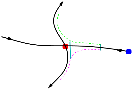
The FTLE field given by $\sigma({\bm{y}},t_{i},T)$ can be shown to exhibit “ridges” of local maxima in phase space. The ridges of the field indicate the location of attracting (backward time FTLE field) and repelling (forward time FTLE field) structures. In two-dimensional (2D) space, the ridge is a curve which locally maximizes the FTLE field so that transverse to the ridge one finds the FTLE to be a local maximum. What is remarkable is that the FTLE ridges correspond to the optimal path trajectories, which is shown heuristically in Sec. 5. The basic idea is that since the optimal path is inherently unstable and observed only through many realizations of stochastic experiments, the FTLE shows that locally, the path is also the most sensitive to initial data. Figure 1 shows a schematic that demonstrates why the optimal path has a local maximum to sensitivity. If one chooses an initial point on either side of the path near the endemic state, the two trajectories will separate exponentially in time. This is due to the fact that both extinct and endemic states are unstable, and the connecting trajectory defining the path is unstable as well. Any initial points starting near the optimal path will leave the neighborhood in short time.

Figure 1: (Color online) Schematic showing the path from the endemic state (blue) to the extinct state (red). The optimal path leaves the endemic point along an unstable manifold and connects to the extinct state along a stable manifold. The magenta and green dashed lines represent trajectories on either side of the optimal path. The initial starting distance between trajectories near the endemic state expands exponentially in forward time (shown by the cyan lines). Locally, this demonstrates that the finite-time Lyapunov measure of sensitivity with respect to initial data is maximal along the optimal path. This is evident in the ridges observed in the evolution of the exponents.

4 Finding the Optimal Path to Extinction Using FTLE

We now apply our theory of dynamical sensitivity to the problem of locating optimal paths to extinction for several examples. We consider the case of internal fluctuations, where the noise is not known a priori, as well as the case of external noise, where the noise is specified. In each case, the interaction of the noise and state of the systems begin with a description of the Hamiltonian (or Lagrangian) to describe the unstable flow. Then the corresponding equations of motion are used to compute the ridges corresponding to maximum FTLE, which in turn correspond to the optimal extinction paths (Schwartz et al., 2010).

4.1 Example 1 - Extinction in a Branching-Annihilation Process

For an example of a system with intrinsic noise fluctuations which has an analytical solution, we consider extinction in the stochastic branching-annihilation process

$$A\xrightarrow{\lambda}2A\quad{\rm and}\quad 2A\xrightarrow{\mu}\emptyset,$$ (14)

where $\lambda$ and $\mu>0$ are constant reaction rates (Elgart and Kamenev, 2004; Assaf et al., 2008). Equation (14) is a single species birth-death process and can be thought of as a simplified form of the Verhulst logistic model for population growth (Nåsell, 2001).

The stochastic process given by Eq. (14) contains intrinsic noise which arises from the randomness of the reactions and the fact that the population consists of discrete individuals. This intrinsic noise, which can generate a rare sequence of events that cause the system to evolve to the empty state, can be accounted for using a master equation approach. The probability $P_{n}(t)$ to observe, at time $t$, $n$ individuals is governed by the following master equation:

$$\dot{P}_{n}=\frac{\mu}{2}\left[(n+2)(n+1)P_{n+2}-n(n-1)P_{n}\right]+\lambda\left[(n-1)P_{n-1}-nP_{n}\right].$$ (15)

Using the formalism of Assaf et al. (2008), Eq. (15) is recast as the following exact evolution equation for $G(\rho,t)$:

$$\frac{\partial G}{\partial t}=\frac{\mu}{2}(1-\rho^{2})\frac{\partial^{2}G}{\partial\rho^{2}}+\lambda\rho(\rho-1)\frac{\partial G}{\partial\rho},$$ (16)

where $G$ is a probability generating function given by

$$G(\rho,t)=\sum\limits_{n=0}^{\infty}\rho^{n}P_{n}(t),$$ (17)

and where $\rho$ is an auxiliary variable.

We substitute the eikonal ansatz $G(\rho,t)={\rm exp}[-\mathcal{S}(\rho,t)]$, where $\mathcal{S}$ is the action, into Eq. (16) and neglect the higher-order $\partial^{2}\mathcal{S}/\partial\rho^{2}$ term. This results in a Hamilton-Jacobi equation for $\mathcal{S}(\rho,t)$. By introducing a conjugate coordinate $q=-\partial\mathcal{S}/\partial\rho$ and by shifting the momentum $p=\rho-1$, then one arrives at the following Hamiltonian:

$$H(q,p)=\left(\lambda(1+p)-\frac{\mu}{2}(2+p)q\right)qp.$$ (18)

Hamilton’s equations are therefore given as:

$$\dot{q}= \frac{\partial H}{\partial p}=q[\lambda(1+2p)-\mu(1+p)q],$$ (19a)

$$\dot{p}= -\frac{\partial H}{\partial q}=p[\mu(2+p)q-\lambda(1+p)].$$ (19b)

The Hamiltonian given by Eq. (18) has three zero-energy curves. The first is the mean-field zero-energy line $p=0$, which contains two hyperbolic points given as $h_{1}=(q,p)=(\lambda/\mu,0)$ and $h_{0}=(q,p)=(0,0)$. The second is the extinction line $q=0$, which contains another hyperbolic point given as $h_{2}=(q,p)=(0,-1)$. The third zero-energy curve is non-trivial and is given as follows:

$$q=\frac{2\lambda(1+p)}{\mu(2+p)}.$$ (20)

The segment of the curve given by Eq. (20) which lies between $-1\leq p\leq 0$ corresponds to a heteroclinic trajectory. As $t$ approaches $-\infty$, the trajectory exits the hyperbolic point $h_{1}$ along its unstable manifold and enters the hyperbolic point $h_{2}$ along its stable manifold as $t$ approaches $\infty$. This heteroclinic trajectory is the optimal path to extinction and describes the most probable (rare) sequence of events which evolves the system from a quasi-stationary state to extinction (Assaf et al., 2008).

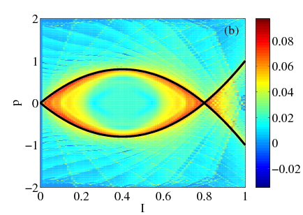
To show that the FTLE evolves to the optimal path, we calculate the FTLE field using Eqs. (19a)-(19b). Figure 2(a) shows the forward FTLE plot computed using Eqs. (19a)-(19b) for $T=6$, with $\lambda=2.0$ and $\mu=0.5$. In Fig. 2(a), one can see that the optimal path to extinction is given by the ridge associated with the maximum FTLE.

Figure 2: (Color online) FTLE flow fields computed using Eqs. (19a)-(19b) with $\lambda=2.0$ and $\mu=0.5$. The integration time is $T=6$ with an integration step size of $t=0.1$ and a grid resolution of $0.01$ in both $q$ and $p$. (a) Forward FTLE field with the optimal path to extinction given by the LCS. (b) Average of the forward and backward FTLE fields with the three zero-energy curves given by the LCS and overlaid with the analytical solution of these curves given by $p=0$, $q=0$, and Eq. (20). Note that the averaging affects only the value of the FTLE and not the structure of the FTLE field.

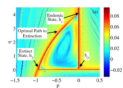
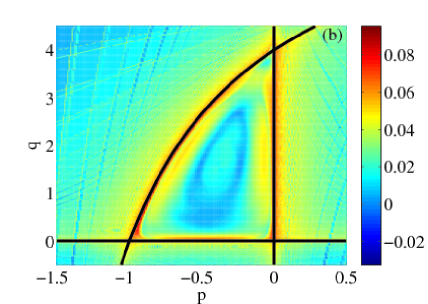
Not all of the attracting structures are shown in Fig. 2(a) because the maximum forward time FTLE identifies repelling structures where nearby initial conditions diverge. The other attracting structures may be found by computing the backward FTLE field. By overlaying the forward and backward FTLE fields, one can see in their entirety all three zero-energy curves including the optimal path to extinction in Fig. 2(b). Also shown in Fig. 2(b) are the analytical solutions to the three zero-energy curves given by $p=0$, $q=0$, and Eq. (20). There is excellent agreement between the analytical solutions of all three curves and the LCS which are found through numerical computation of the FTLE flow fields.

4.2 Example 2 - SIS Epidemic Model - External Fluctuations

As another general application of the extinction theory for finite populations, we consider the well-known problem of extinction in a Susceptible-Infectious-Susceptible (SIS) epidemiological model. The SIS model is given by the following system of equations:

$$\dot{S}= \mu-\mu S+\gamma I-\beta IS,$$ (21a)

$$\dot{I}= -(\mu+\gamma)I+\beta IS,$$ (21b)

where $\mu$ represents a constant birth and death rate, $\beta$ represents the contact rate, and $\gamma$ denotes the rate of recovery. If we assume that the total population size is constant and can be normalized to $S+I=1$, then Eqs. (21a)-(21b) can be rewritten as the following one-dimensional (1D) equation:

$$\dot{I}=-(\mu+\gamma)I+\beta I(1-I).$$ (22)

Figure 3: (Color online) FTLE flow fields computed using Eqs. (28a)-(28b) with $\beta=5.0$ and $\kappa=1.0$. The integration time is $T=5$ with an integration step size of $t=0.1$ and a grid resolution of $0.01$ in both $I$ and $p$. (a) Forward FTLE field with the optimal path to extinction given by the LCS. (b) Average of the forward and backward FTLE fields with the optimal path to extinction and its counterpart optimal path given by the LCS and overlaid with the analytical solution of the optimal paths given by Eq. (27). Note that the averaging affects only the value of the FTLE and not the structure of the FTLE field.

The stochastic version of Eq. (22) is given as

$$\dot{I}=-(\mu+\gamma)I+\beta I(1-I)+\eta(t)=F(I)+\eta(t),$$ (23)

where $\eta(t)$ is uncorrelated Gaussian noise with zero mean and models random migration to and from another population (Alonso et al., 2006; Doering et al., 2005). Equation (23) has two equilibrium points given by $I=0$ (corresponding to the disease-free state) and $I=1-(\mu+\gamma)/\beta$ (corresponding to the endemic state). One can use the Euler-Lagrange equation of motion to find the optimal path of extinction from the endemic state to the disease-free state, where the Lagrangian is determined by Eq. (23) and is given as follows:

$$L(I,\dot{I})=[\eta(t)]^{2}=[\dot{I}-F(I)]^{2}.$$ (24)

Computation of the Euler-Lagrange equation gives the following:

$$F(I)F^{\prime}(I)-\ddot{I}=0.$$ (25)

If one multiplies Eq. (25) by $\dot{I}$ followed by an integration with respect to $t$, then one obtains

$$\frac{F(I)^{2}}{2}-\frac{\dot{I}^{2}}{2}=E,$$ (26)

where $E$ is an arbitrary constant. Using the fact that the optimal path passes through the two equilibrium points stated above, then one finds that the optimal path to extinction (as well as its counterpart path from the disease-free state to the endemic state) is given by the following equation:

$$\dot{I}=\pm F(I).$$ (27)

As in the first example, one can numerically compute the optimal path to extinction using the FTLE. In this example we calculate the FTLE field using the following 2D system which is equivalent to Eq. (25):

$$\dot{I}= p,$$ (28a)

$$\dot{p}= F(I)F^{\prime}(I)=(\beta I(1-I)-\kappa I)(\beta(1-2I)-\kappa),$$ (28b)

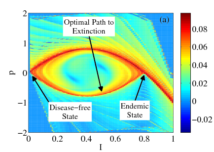
where $\kappa=\mu+\gamma$. Figure 3(a) shows the forward FTLE plot computed using Eqs. (28a)-(28b) for $T=5$, with $\beta=5.0$ and $\kappa=1.0$. In Fig. 3(a), one can see that the optimal path from the endemic state to the disease-free state is given by the ridge associated with the locally maximal FTLE.

One also can find the optimal path from the disease-free state to the endemic state by computing the backward FTLE. By overlaying the forward and backward FTLE fields, one can see the optimal path to extinction along with its counterpart optimal path in Fig. 3(b). Also shown in Fig. 3(b) are the two analytical solutions to the optimal path to extinction and its counterpart optimal path which are given by Eq. (27). There is excellent agreement between the analytical solutions to the two optimal paths and the ridges which are found through numerical computation of the FTLE flow fields.

4.3 Example 3 - SIS Epidemic Model - Internal Fluctuations

We now consider the 1D stochastic (internal) version of the SIS epidemic model given by Eq. (22). The probability $P_{n}(t)$ to observe, at time $t$, $n$ infectious individuals is governed by the following master equation:

$$\dot{P}_{n}=(\mu+\gamma)[(n+1)P_{n+1}-nP_{n}]+\beta[(n-1)(1-(n-1))P_{n-1}-n(n-1)P_{n}].$$ (29)

Using the formalism of Gang (1987), one then has the following Hamiltonian associated with Eq. (29):

$$H(I,p)=(\mu+\gamma)I(e^{-p}-1)+\beta I(1-I)(e^{p}-1),$$ (30)

and Hamilton’s equations are therefore given as:

$$\dot{I}= \frac{\partial H}{\partial p}=-(\mu+\gamma)Ie^{-p}+\beta I(1-I)e^{p},$$ (31a)

$$\dot{p}= -\frac{\partial H}{\partial I}=-(\mu+\gamma)(e^{-p}-1)+\beta(e^{p}-1)(2I-1).$$ (31b)

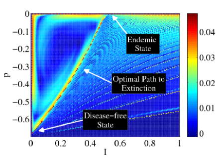
Although there is no analytical solution for the optimal path to extinction for Eqs. (31a)-(31b), we can once again determine the optimal path by computing the FTLE flow field associated with this system. Figure 4 shows the forward FTLE plot computed using Eqs. (31a)-(31b) for $T=10$, with $\beta=2.0$ and $\kappa=1.0$. As we have seen previously, the optimal path to extinction from the endemic state to the disease-free state is given by the ridge associated with the locally maximal FTLE.

Figure 4: (Color online) FTLE flow field computed using Eqs. (31a)-(31b) with $\beta=2.0$ and $\kappa=1.0$. The integration time is $T=10$ with an integration step size of $t=0.1$ and a grid resolution of $0.005$ in both $I$ and $p$. The optimal path to extinction is given by the LCS.

5 Maximal Sensitive Dependence to Initial Data Near the Optimal Path

The main heuristic argument of this section is to show that the path which maximizes the probability of extinction also has a finite-time Lyapunov exponent (FTLE) that attains its local maximum on the path. We consider a general system of equations and show how the maximum unstable direction along the optimal path to extinction governs the local hyperbolic dynamics.

From the Hamiltonian or Lagrangian equations of motion, the process which leads to extinction consists of a trajectory which emanates from a stable steady state ${\bm{x}}_{a}\in{\mathbb{R}}^{n}$ and approaches the extinct state ${\bm{x}}_{s}\in{\mathbb{R}}^{n}$. Since the stable and extinct states are both regular saddles (or unstable foci) in the variational formulations, they both have hyperbolic structure. Moreover, every point along the trajectory connecting the two states as $t\rightarrow\pm\infty$ is assumed to possess a local hyperbolic structure. As an example, consider the Langevin problem having a vector field of position ${\bm{V}}:{\mathbb{R}}^{n}\rightarrow{\mathbb{R}}^{n}$, which has the associated Lagrangian $L({\bm{x}},\dot{\bm{x}})=\left\|\dot{{\bm{x}}}-{\bm{V}}({\bm{x}})\right\|{}^{2}/2$ to describe the action. Converting to a Hamiltonian formulation leads one to the following $2n$-dimensional equations of motion and Hamiltonian:

$$\dot{\bm{x}}={\bm{p}}+{\bm{V}}({\bm{x}}),$$ (32a)

$$\dot{\bm{p}}=-{\bm{V}}^{\prime}({\bm{x}}){\bm{p}},$$ (32b)

$$H({\bm{x}},{\bm{p}})=\frac{\left\|{\bm{p}}\right\|^{2}}{2}+{\bm{p}}\cdot{\bm{V}}({\bm{x}}),$$ (32c)

where $\bm{V}^{\prime}(\bm{x})\equiv\frac{\partial{\bm{V}}(\bm{x})}{\partial{\bm{x}}}$ is the Jacobian matrix evaluated at ${\bm{x}}$.

It is immediate from Eqs. (32a)-(32c) that $\left\{({\bm{x}},{\bm{p}})\,|\,\,{\bm{p}}={\bm{0}}\right\}$ is an invariant manifold. In addition, the optimal path must lie along the $H({\bm{x}},{\bm{p}})=0$ surface, which means that in addition to the ${\bm{p}}={\bm{0}}$ manifold, the zero surface includes $\left\{({\bm{x}},{\bm{p}})\,|\,\,{\bm{p}}=-2{\bm{V}}({\bm{x}})\right\}$.

To clarify the direction along the optimal path as well as the local geometry, we make the following assumptions regarding ${\bm{V}({\bm{x}})}$:

1. ${\bm{V}}({\bm{x}})$ is smooth,

2. ${\bm{V}}({\bm{x}_{a}})={\bm{V}}({\bm{x}}_{s})={\bm{0}}$,

3. ${\bm{V}}^{\prime}({\bm{x}}_{a})$ has eigenvalues with negative real parts, and ${\bm{V}}^{\prime}({\bm{x}}_{s})$ has at least one eigenvalue with positive real part.

Items 2 and 3 imply that ${\bm{x}}_{a}$ is an attracting steady state and ${\bm{x}}_{s}$ is an unstable steady state in the deterministic dynamical system. We now assume that the optimal path must satisfy $\mathop{\lim}\limits_{t\to+\infty}({\bm{x}}(t),{\bm{p}}(t))=({\bm{x}}_{s},{\bm{0}})$, while $\mathop{\lim}\limits_{t\to-\infty}({\bm{x}}(t),{\bm{p}}(t))=({\bm{x}}_{a},{\bm{0}})$. Since $H({\bm{x}}(t),{\bm{p}}(t))=0$ along the path, the limits provide direction along the optimal path.

The optimal path lies on the curve

$$C_{({\bm{x}},{\bm{p}})}=\left\{t\in(-\infty,\infty)\,|\,{\bm{p}}(t)=-2{\bm{V}}({\bm{x}}(t))\right\},$$

and ${\bm{p}}={\bm{0}}$ corresponds to the zero fluctuation case. We shift the optimal path to the origin by using the following $2n$-dimensional transformation:

$${\bm{u}}={\bm{x}},$$ (33a)

$${\bm{w}}={\bm{p}}+2{\bm{V}}({\bm{x}}),$$ (33b)

$$\hat{H}({\bm{u}},{\bm{w}})=\frac{\left\|{\bm{w}}\right\|^{2}}{2}-{\bm{w}}\cdot{\bm{V}}(\bm{u}).$$ (33c)

The new equations of motion are now:

$$\dot{\bm{u}}=\partial\hat{H}/\partial{\bm{w}}={\bm{w}}-{\bm{V}}({\bm{u}}),$$ (34a)

$$\dot{\bm{w}}=-\partial\hat{H}/\partial{\bm{u}}={\bm{V}}^{\prime}({\bm{u}}){\bm{w}}.$$ (34b)

The optimal path now is described by the curve

$$C_{({\bm{u}},{\bm{w}})}=\left\{t\in(-\infty,\infty)\,|\,{\bm{w}}(t)={\bm{0}},\dot{\bm{u}}(t)=-{\bm{V}}({\bm{u}}(t))\right\},$$

while the zero fluctuation case given by ${\bm{p}}={\bm{0}}$ now corresponds to ${\bm{w}}=2{\bm{V}}({\bm{u}})$.

The linearized variation along the optimal path $C_{({\bm{u}},{\bm{w}})}$ is given by the following matrix initial value problem from Eqs. (34a)-(34b):

$$\dot{{\bm{X}}}=\left[\begin{array}[]{cc}-{\bm{V}}^{\prime}({\bm{u}}(t))&{\bm{I}}_{n}\\ {\bm{0}}&{\bm{V}}^{\prime}({\bm{u}}(t))\end{array}\right]{\bm{X}}\equiv{\bm{J}}({\bm{u}}(t),{\bm{0}}){\bm{X}},\quad{\bm{X}}({\bm{0}})={\bm{I}}.$$ (35)

For a fixed time $t_{0}$ such that ${\bm{u}}(t_{0})={\bm{u}}_{0}$, the local eigenvalues of Eq. (35) are given by the eigenvalues of $\pm{\bm{V}}^{\prime}({\bm{u}}_{0})$ and are assumed to have non-zero real part for any $({\bm{u}}_{0},{\bm{0}})\in C_{({\bm{u}},{\bm{w}})}$. Thus the optimal path is hyperbolic at every point. We also suppose the existence of a local coordinate system on the path so that there exists a set of linearly independent directions pointwise.

The solution to the linear variational equation about $({\bm{u}},{\bm{w}})=({\bm{u}}_{0},{\bm{0}})$ for $0<t\ll 1$ is given by ${\bm{X}}(t)\approxeq\exp{(t{\bm{J}}({\bm{u}}_{0},{\bm{0}}))}$. We assume for simplicity that the eigenvalues of ${\bm{V}}^{\prime}(u_{0})$ have algebraic multiplicity of one. The eigenvalues of ${\bm{J}}({\bm{u}}_{0},{\bm{0}})$ are given by $\{\pm\lambda_{i}\}_{i=1}^{n}$, where $\lambda_{i}$ are eigenvalues of ${\bm{V}}^{\prime}({\bm{u}}_{0})$. To examine the dynamic instability that dominates locally, let $\lambda_{{\rm max}}$ denote the eigenvalue with largest real part and be such that $Re(\lambda_{max})>0$. Since $-\lambda_{{\rm max}}$ has the most negative real part, its eigendirection denotes the strongest contracting direction.

For any $({\bm{u}}_{0},{\bm{0}})$ on the path, the existence of a set of linearly independent eigensolutions of ${\bm{J}}({\bm{u}}_{0},{\bm{0}})$ implies there is a transformation ${\bm{X}}={\bm{P}}{\bm{Y}}$, with $\bm{P}\in{\mathbb{L}}^{2n\times 2n},$ that diagonalizes the linear variational equation given by Eq. (35). Without loss of generality, we can also assume that the diagonal consists of ordered descending eigenvalues based on the real part. Therefore, the linear variational system has the form

$$\dot{\bm{Y}}=\left[\begin{array}[]{cccccc}\lambda_{{\rm max}}\\ &\ddots\\ &&\lambda_{n}\\ &&&-\lambda_{n}\\ &&&&\ddots\\ &&&&&-\lambda_{{\rm max}}\end{array}\right]{\bm{Y}}.$$ (36)

For any initial value, the solution to Eq. (36) is

$${\bm{x}}_{p}(t;{\bm{x}}_{0}) =(x_{1}(t),x_{2}(t),\cdots,x_{2n}(t))$$ (37)

$$=(e^{\lambda_{{\rm max}}t}x_{10},e^{\lambda_{2}t}x_{20},\cdots,e^{\lambda_{n}t}x_{n0},$$

$$\qquad\quad e^{-\lambda_{n}t}x_{(n+1)0},\cdots,e^{-\lambda_{2}t}x_{(2n-1)0},e^{-\lambda_{{\rm max}}t}x_{2n0}).$$ (38)

To show that the FTLE takes it maximum along the path, we notice that any point along the path is hyperbolic with a saddle structure. Therefore, we consider an arbitrary initial condition lying within a small domain containing the origin. Since almost any initial condition hits the boundary of the domain in finite time due to the saddle structure of the origin, we use the escape time as the final time for the FTLE. The definition we use of the FTLE is the direct comparison of the distance between two close trajectories as follows:

$$\sigma(t;{\bm{x}}_{0})=\frac{1}{t}\ln{(||{\bm{x}}_{p}(t;{\bm{x}}_{0}+{\bm{\epsilon}})-{\bm{x}}_{p}(t;{\bm{x}}_{0})||)},$$ (39)

where ${\bm{\epsilon}}\in{\mathbb{R}}^{2n}$.

Defining the domain to be the $2n$-dimensional hypercube $D=[-1,1]^{2n}$, then clearly any point not on the unstable manifold will escape in the $x_{1}$ direction corresponding to the eigenvalue with maximal real part. We exploit the fact that the dynamics is governed by the most unstable direction by assuming $\left|\lambda_{{\rm max}}\right|>>\left|\lambda_{i}\right|$, $i=2\cdots n$. If the initial condition lies within a distance $\delta$ of the unstable manifold with $0<\delta<<1$, then the time to escape from the domain for an arbitrary non-zero initial condition is given by

$$t_{f}\approxeq-\frac{\log{(\delta)}}{\lambda_{{\rm max}}}.$$ (40)

Using the definition of the exponent given by Eq. (39), we have that

$$\sigma(t_{f},{\bm{x}}_{0})= -\lambda_{{\rm max}}\ln{\left(\left|\frac{\epsilon_{1}}{\delta}\right|^{2}+\left|\delta^{-\frac{\lambda_{2}}{\lambda_{{\rm max}}}}\epsilon_{2}\right|^{2}+\cdots+\left|\delta^{-\frac{\lambda_{n}}{\lambda_{{\rm max}}}}\epsilon_{n}\right|^{2}+\left|\delta^{\frac{\lambda_{n}}{\lambda_{{\rm max}}}}\epsilon_{n+1}\right|^{2}\right.}$$

$$\left.+\cdots+\left|\delta^{\frac{\lambda_{2}}{\lambda_{{\rm max}}}}\epsilon_{2n-1}\right|^{2}+\left|\delta\epsilon_{2n}\right|^{2}\right)/\left(2\ln{(\delta)}\right).$$ (41)

Since $\left|\lambda_{{\rm max}}\right|>>\left|\lambda_{i}\right|$, and since $\pm\lambda_{{\rm max}}$ dominates the expanding and contracting directions, then for $\delta$ small, we may just consider

$$\sigma(t_{f},{\bm{x}}_{0})=\frac{-\lambda_{{\rm max}}\ln{(\epsilon_{1}^{2}/\delta^{2}+\epsilon_{2n}^{2}\delta^{2})}}{2\ln{\delta}}.$$ (42)

Furthermore, we find that

$$\frac{\partial\sigma(t_{f};{\bm{x}}_{0}(\delta))}{\partial\delta}={\frac{\lambda_{{\rm max}}\,\ln\left({\epsilon}_{1}^{2}\right)}{2\delta\left(\ln{\delta}\right)^{2}}}\left(1+\frac{\delta^{4}\epsilon_{2n}^{2}}{\epsilon_{1}^{2}}\right)+\mathcal{O}\left(\frac{\delta^{3}}{\ln{\delta}}\right),\$$ (43)

which can be shown to be negative assuming $\epsilon_{1}<<1$. Therefore, the FTLE as a function of distance to the stable invariant manifold is a decreasing function, and thus takes it maximum values on the manifold.

6 Conclusions

In this article, we have considered the dynamics of general stochastic epidemic models and their extinction properties in finite populations. The random fluctuations considered were from both internal fluctuations, which arise from mass action kinetics, as well as external random forces, which may be due to random population migrations. By examining the extinction processes from the master equation perspective, eikonal approximations in the large population limit give a way to solve for the probability distribution as a function of time. A variational principle applied to the exponent of the probability distribution near the steady state was used to maximize the probability to extinction from a disease endemic state.

Maximizing the probability to extinction means minimizing the action, which in turn generates a Hamiltonian (or Lagrangian) formulation that determines the flow from endemic to extinct states. The formulation describes the random fluctuations as a deterministic effective force that overcomes the instability of the extinct state. Such a deterministic flow describes the optimal path to extinction from an endemic state. Using the above variational formulation, we explicitly derived the equations of motion describing the optimal path to extinction in three different models from epidemiology as a two point boundary value problem

Figure 5: (Color online) Snapshots taken at (a) $t=1$, (b) $t=3$, (c) $t=5$, (d) $t=7$, and (e) $t=9$ showing the evolution of the FTLE flow field computed using Eqs. (31a)-(31b) with $\beta=2.0$ and $\kappa=1.0$. The integration time is $T=10$ with an integration step size of $t=0.1$ and a grid resolution of $0.005$ in both $I$ and $p$. The final snapshot in the series is taken at $t=10$ and is shown in Fig. 4. A video that shows the evolution of the FTLE flow field can be found online as ancillary material.

The main result of our paper is that the optimal path is intimately related to the maximal sensitivity of the dynamics of unstable Hamiltonian flows. Specifically, we introduced a novel method to find the optimal path to extinction that relies on the computation of the finite-time Lyapunov exponent field for the dynamical flow under consideration. The exponents provide a measure of sensitivity to initial conditions in finite time. Moreover, we have shown that the system possesses maximal sensitivity near the optimal path to extinction. Therefore, we are able to use the finite-time Lyapunov exponents to dynamically evolve toward the optimal path trajectory.

To demonstrate the equivalence of the maximal sensitivity and the optimal path maximizing the probability of extinction, we have considered three prototypical examples from mathematical epidemiology. In the examples, we have considered both internal and external noise, and we have considered both a Hamiltonian and Lagrangian formulation. Furthermore, in each of the three examples, we have shown that the optimal path to extinction is equated with having a (locally) maximal sensitivity to initial condition, which implies a relation at a fundamental level between the optimal path and the FTLE. Even though there exist many possible paths to extinction, the dynamical systems approach converges to the path that maximizes the probability to extinction.

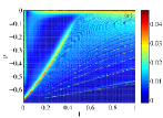
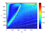
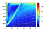
An example of the evolution of the FTLE flow field showing the convergence of the locally maximal FTLE ridge to the optimal path is shown in Fig. 5. The FTLE flow field is computed for $T=10$ using Eqns. (31a)-(31b) for the SIS epidemic model with internal fluctuations (Sec. 4.3). Figure 5 shows snapshots of the FTLE field taken at $t=1$, $t=3$, $t=5$, $t=7$, and $t=9$. The final snapshot at $t=10$ is shown in Fig. 4. A video that shows the evolution of the FTLE flow field can be found online as ancillary material.

The parameter values chosen for the three examples are such that the extinct and endemic states are far away from one another, implying that the system is operating far from any bifurcation points. This result is very important, since in general, no approximate analytical treatment, like the one performed in Dykman et al. (2008), is possible if the system’s dynamics is not sufficiently close to the bifurcation point. However, any scaling behavior of the exponent in the probability of extinction may still be computed along the optimal path, which is the important advance afforded by the new procedure proposed in this paper.

In the future, we plan on considering more complicated systems. Of particular interest are bistable systems (e.g. adaptive networks (Shaw and Schwartz, 2008) and the Schlögl birth-death process (Doering et al., 2007)), and higher-dimensional systems (e.g. multistrain epidemic models (Shaw et al., 2007)). Because the method is general, and unifies dynamical systems theory with the probability of extinction, we expect that any system found in other fields can be understood using this approach.