From coupled elementary units to the complexity of the glass transition
Abstract
Supercooled liquids display fascinating properties upon cooling such as the emergence of dynamic length scales. Different models strongly vary with respect to the choice of the elementary subsystems (CRR) as well as their mutual coupling. Here we show via computer simulations of a glass former that both ingredients can be identified via analysis of finite-size effects within the continuous-time random walk framework. The CRR already contain complete information about thermodynamics and diffusivity whereas the coupling determines structural relaxation and the emergence of dynamic length scales.
pacs:
61.20.Lc, 61.20.Ja, 64.70.pmUnderstanding the complex dynamics of supercooled liquids down to the glass transition as reflected, e.g., by the emergence of dynamic length scales L. Berthier et. al (2005); Stein and Andersen (2008) is still a highly controversal problem P. G. Debenedetti and F. H. Stillinger (2001); Dyre (2006). Qualitatively speaking the system decomposes into coupled elementary units (sometimes denoted cooperatively rearranging regions (CRRs) Adam and Gibbs (1965)). Presently discussed models differ dramatically with respect to the nature of this decomposition. For example in the mosaic approach Kirkpatrick et al. (1989); Xia and Wolynes (2001a, b); Lubchenko and Wolynes (2006) the complexity is fully embedded in the properties of the CRRs, denoted mosaics, whereas in the other extreme of the kinetically constrained models (KCMs) Fredrickson and Andersen (1984); Garrahan and Chandler (2002); Jung et al. (2004); Hedges et al. (2009) the complexity is exclusively is related to the coupling while the elementary units are just trivial two-state systems.
Here we show that it is possible via computer simulations of a standard model glass former to obtain a clear-cut decomposition and thus to learn about the nature of the CRRs as well as the coupling between them. The key idea is to directly extract coupling effects from studying the size-dependence under periodic boundary conditions. The analysis is performed in the continuous-time random walk (CTRW) framework which for the first time is quantitatively extended to larger systems. Two conclusions can be drawn. Firstly, our results explain the fact that the structural relaxation time displays major finite size effects whereas there are hardly any for the diffusion constant. Secondly, we present a minimum model of the glass transition which reflects the observed coupling effects. Albeit similar in spirit to the KCMs many important differences are present.
We have simulated the binary mixture Lennard-Jones system (BMLJ) which can be regarded as a prototype glass-former Kob and Andersen (1995). Simulations have been performed in the NVT ensemble. For the smaller system we have have used a slightly shorter cutoff of Doliwa and Heuer (2003a). In previous work it has been shown that a system as small as particles with periodic boundary conditions basically displays very similar thermodynamic as well as diffusive properties as a macroscopic system in the range of temperatures, accessible to computer simulations (in particular between and ) Doliwa and Heuer (2003b). Interestingly, for the same temperature range is too small Buechner and Heuer (1999). Thus, a BMLJ system with is close to a system reflecting the effects of just a single CRR (more precisely: two CRRs Heuer et al. (2005)).
Due to the microscopic resolution computer simulations are very well suited to extract relevant information about the coupling effects. One route which has been chosen by Biroli et al. is to immobilize a large system except for a sphere of variable radius and to study the dynamics in this sphere in dependence of Biroli et al. (2008). One faces the problem to extract from this highly non-equilibrium situation the relevant equilibrium properties. In this work we analyze the size-dependence of the BMLJ system. From the perspective of a CRR the coupling effects are switched on when increasing the system size. Interestingly, the structural relaxation time Stariolo and Fabricius (2006); Karmakar et al. (2009) as well as the length scale of dynamic heterogeneities display significant finite-size effects Whitelam et al. (2004); Berthier and Jack (2007).
A key observable to characterize the relaxation is the incoherent scattering function which is defined as
| (1) |
where denotes the single-particle displacement vector during time . The contribution of structural relaxation to the decay of can be determined by referring to the inherent structure (IS) trajectory, obtained after minimizing every configuration Schrøder et al. (2000), reflecting the minima of the potential energy landscape (PEL) Wales (2003). The resulting incoherent scattering function is denoted . Qualitatively, this procedure corresponds to a removal of the vibrational contributions. Conceptually similar is the use of the metabasin (MB) trajectory P. G. Debenedetti and F. H. Stillinger (2001); Doliwa and Heuer (2003b); Heuer (2008). A MB consists of an appropriately chosen set of nearby IS. The k-dependent relaxation time, which reflects the time a particle on average needs to move the distance , is defined via .
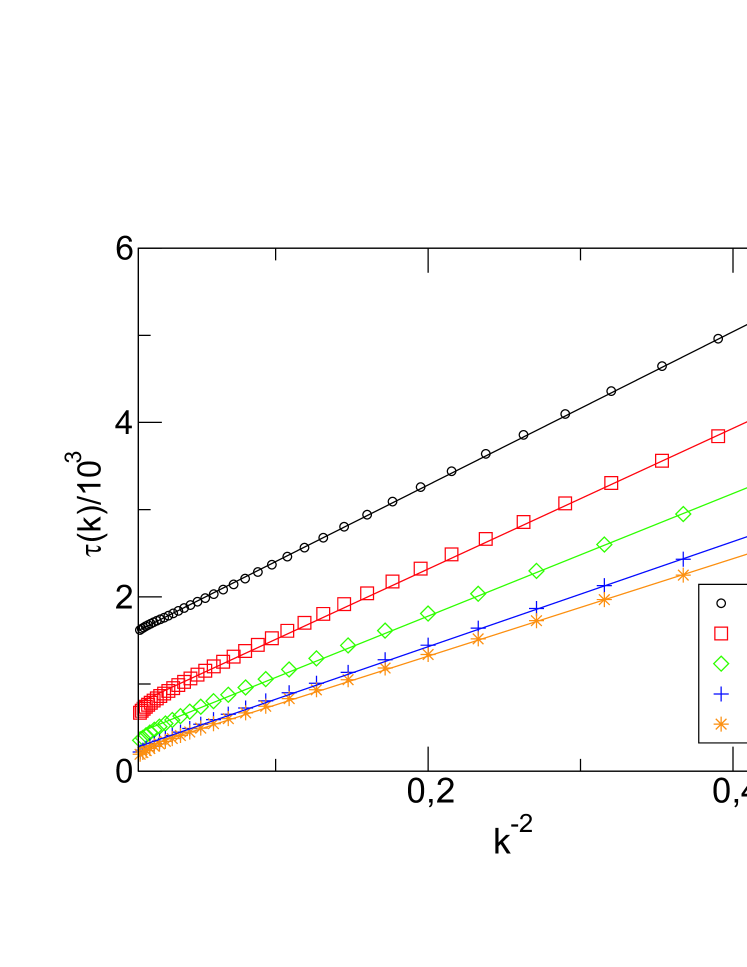
In Fig.1 we show the wave vector dependent relaxation time based on where the large k limit is significantly beyond the maximum of the structure factor. As shown in Rubner and Heuer (2008) the metabasin (MB) dynamics of a system with can be described as a CTRW in configuration space (with waiting times ) where spatial and temporal properties are decoupled Rubner and Heuer (2008). As a consequence the k-dependence of can be written as Berthier et al. (2005); Rubner and Heuer (2008)
| (2) |
where Berthier et al. (2005); Rubner and Heuer (2008)
| (3) |
Due to the presence of dynamic heterogeneities, the distribution of waiting times is very broad so that .
How to characterize the dynamics for large systems ()? In this limit the MB trajectory would violate one of the crucial assumptions of the CTRW approach because due to the dynamic heterogeneities successive MB transitions are often performed by identical particles Rubner and Heuer (2008). In particular, Eq.3 is no longer valid for large . There exists, however, an elegant solution to this problem by defining local waiting times on the single-particle level in real space Vollmayr-Lee (2004); Hedges et al. (2007). Specifically, one considers a trajectory which is time-averaged for a time somewhat longer than the vibrational time scale. Whenever the particle has moved a fixed distance (here: in LJ-units where the precise choice is irrelevant) one identifies a transition process.
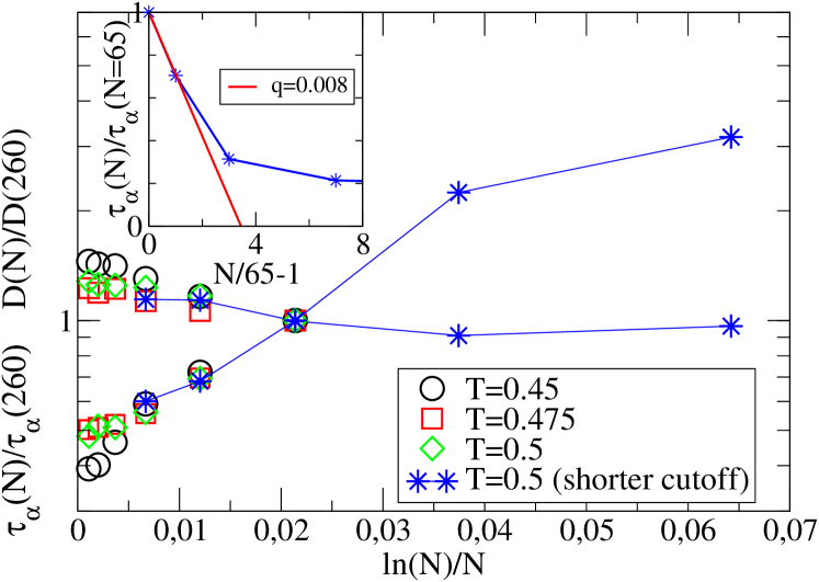
Validity of the CTRW-behavior in configuration space implies that the corresponding single-particle trajectories can be also described as a CTRW where Eq.3 has to be modified by replacing with . One might expect that this CTRW-type single-particle dynamics should prevail also when increasing the system size. Indeed, as can be seen from Fig.1 Eq.2 is applicable for all in the complete -range under consideration. In Fig.2 the resulting values of and are shown for different temperatures. Note that the diffusion constant indeed only displays small finite size effects whereas the relaxation time varies by nearly one order of magnitude. At first glance this may seem somewhat counterintuitive because upon decreasing the system size major finite-size effects are observed for a small-scale (large ) observable, i.e. , but not for a large-scale (small ) observable, i.e. .
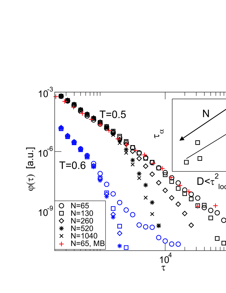
Finally, we analyse the -dependence of as shown in Fig. 3. The data are discussed in three different directions. First, for and we have also included showing a very good agreement with , thereby supporting the mapping of the waiting times in configuration space to those in real space. The presence of a few extremely long waiting times reflects the fact that on average a MB transition only covers half of the system size Heuer et al. (2005). Thus, there is a finite probability that some particles remain immobile even longer than the longest MB waiting time. Second, in the inset of Fig.3 we verify the relation in Eq.3 within statistical uncertainty. Third, one clearly sees that long residences of slow particles are strongly suppressed when approaching the large-size limit. This observation is particularly pronounced for the lower temperature where up to particles finite-size effects are present. One might be tempted to conclude that the additional fluctuations around a given subsystem increase the mobility and shifts all time scales to shorter times. This, however, disagrees with the very small finite-size effects of the diffusion constant which implies that the first moment of the waiting time distribution is basically unchanged.
For a system with it has been shown that the state of the system can be, to a reasonable approximation, characterized by a rate , denoting the probability for a MB transition Heuer et al. (2005); Heuer (2008). To discuss the nature of the observed finite-size effects we assume for reasons of simplicity that this approximation is strictly valid. Furthermore we introduce as the equilibrium distribution of rates. A finite width of is equivalent to the presence of dynamic heterogeneities. For it turns out that is strongly related to the MB energy Heuer (2008). Thus, the observed invariance of the thermodynamic properties, i.e. the trivial scaling of (e: MB energies) upon increasing the system size, strongly suggests that for the subsystem does not change either. This also follows from the previously reported observation that in terms of MB transitions the total system behaves as if it were a superposition of independent subsystems of size Doliwa and Heuer (2003c). As a consequence the remaining effect of the coupling is to give rise to fluctuations of the rate of the tagged subsystem due to relaxation processes in adjacent subsystems without modifying the overall distribution (passive exchange process).
This coupling has one important consequence. During a very immobile period, characterized by a small value of , it is very likely that the system acquires a new (and on average larger) value of . This immediately explains the numerical observation that the long-time contribution to disappears when the system size increases and thus the fluctuations become faster.
Furthermore, these observations allow us to understand the nature of the finite-size effects of . In particular one needs to understand why finite-size effects occur for rather than . Both observables are fundamentally different because (at least for spatially uncorrelated jumps) the diffusivity is fully determined by the properties of a single jump whereas for complete structural relaxation basically every particle has to move, requiring a large number of elementary relaxation processes. Thus, the presence of passive exchange processes is relevant for but not for . A more formal description of the resulting differences can be achieved by using the relations and where the average is over Diezemann et al. (1998). For reasons of simplicity we consider the case where the fluctuations of are extremely fast. Naturally, these fluctuations leave the average rate and thus unchanged. For , however, needs to be substituted by . Then one obtains
| (4) |
where the inequality is a strict mathematical statement if dynamic heterogeneities are present. Of course, the less pronounced the fluctuations the smaller the ratio .
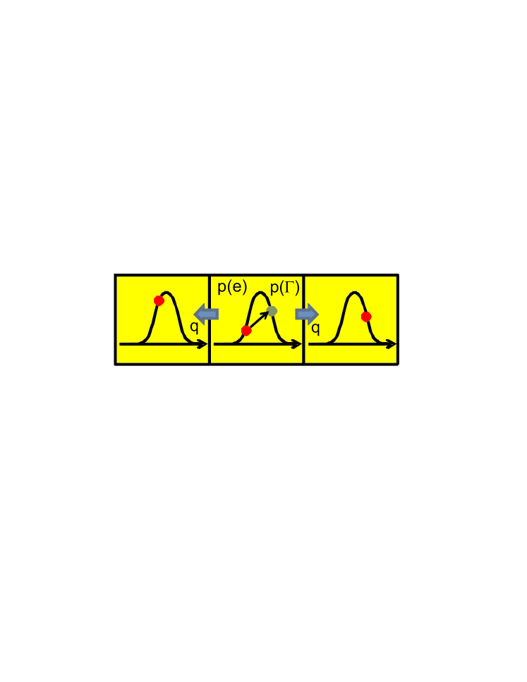
A simple visualization of the physical scenario is presented in Fig. 4: (1) The local system of size fully contains the information about the thermodynamics as well as the diffusion constant (first moment of waiting time distribution). This system can be very well characterized in the MB framework (given and ). Since, at least in the analyzed temperature range, is roughly temperature-independent no dynamic length scales are involved to characterize, e.g., the temperature dependence of the diffusion constant.(2) The macroscopic system can be regarded as a superposition of systems of size . The coupling is too weak to change the thermodynamics (basically, this was the criterion to define ) but gives rise to a dynamic coupling between the subsystems. For the minimum model, sketched in Fig. 4 one can directly estimate the coupling constant in the limit of small and not too large sup via the relation
| (5) |
with and for the present system as determined in Ref. Rubner and Heuer (2008) in the CTRW context. Comparison with the numerical data yields , see Fig.2. This clearly shows that efficient coupling does not occur on the time scale of MB transitions but for the present case on the time scale of .
The resulting correlations between the mobilities of adjacent systems will lead to the emergence of temperature-dependent length scales of dynamic heterogeneities. These correlations do not show up via a spatial correlation of instantaneous rates but rather from the spatial correlation of the relaxation behavior during sufficiently long time intervals (e.g. of the order of ), as exactly captured by the four-point correlation function Glotzer et al. (2000). For a simple model system one can show sup how the coupling modifies the value of and how dynamic correlations and thus dynamic length scales emerge.
The aspect of coupling is rephrased in the KCMs in a schematic way. Thus it is not surprising that several similarities to atomic glass-formers exist (e.g. in the FA model the diffusion constant does not depend on the coupling and the elementary length scale, i.e. a spin, is temperature-independent Jung et al. (2004)). However, some important differences remain. (1) Whereas a system of size , representing approx. two elementary units, already reflects many features of the macroscopic system, the same number of spins in the KCM naturally does not display any relevant behavior. (2) In principle a subsystem can always relax without constraints by its neighbors (see also Ref.Hedges et al. (2009)) since the coupling is via passive exchange processes rather than yes/no-decisions. (3) Strong and fragile systems can be understood by the same coupling rules by just changing the properties of the potential energy landscape of the subsystems Heuer (2008) whereas for the KCMs different rules have to be formulated. (4) The experimentally observed correlation between thermodynamic and dynamic properties is kept whereas the thermodynamics is considered irrelevant in the KCM approach. (5) The coupling strength can be directly extracted from simulations of a atomistic glass-forming system, allowing a semi-quantitative mapping between system and model.
In summary, the model, sketched above, can be, on the one hand, regarded as a generalization of the KCM whereas, on the other hand, it is a minimum model, capturing a realistic version of the facilitation effect. In particular it is compatible with the thermodynamic and dynamic observations for the model glass former reported in this work. We just note that there is no obvious way to map the present results on the mosaic approach since the basic length scale, i.e. the scale of the mosaics, is strongly temperature dependent.
We greatly acknowledge the financial support by the DFG (SFB 458).
References
- L. Berthier et. al (2005) L. Berthier et. al, Science 310, 1797 (2005).
- Stein and Andersen (2008) R. S. L. Stein and H. C. Andersen, Phys. Rev. Lett. 101, 267802 (2008).
- P. G. Debenedetti and F. H. Stillinger (2001) P. G. Debenedetti and F. H. Stillinger, Nature 410, 259 (2001).
- Dyre (2006) J. C. Dyre, Rev. Mod. Phys. 78, 953 (2006).
- Adam and Gibbs (1965) G. Adam and J. H. Gibbs, J. Chem. Phys. 43, 139 (1965).
- Kirkpatrick et al. (1989) T. R. Kirkpatrick, D. Thirumalai, and P. G. Wolynes, Phys. Rev. A 40, 1045 (1989).
- Xia and Wolynes (2001a) X. Xia and P. G. Wolynes, Phys. Rev. Lett. 86, 5526 (2001a).
- Xia and Wolynes (2001b) X. Xia and P. G. Wolynes, J. Phys. Chem. B 105, 6570 (2001b).
- Lubchenko and Wolynes (2006) V. Lubchenko and P. G. Wolynes, Ann. Rev. Phys. Chem. 58, 235 (2006).
- Fredrickson and Andersen (1984) G. H. Fredrickson and H. C. Andersen, Phys. Rev. Lett. 53, 1244 (1984).
- Garrahan and Chandler (2002) J. P. Garrahan and D. Chandler, Phys. Rev. Lett. 89, 035704 (2002).
- Jung et al. (2004) Y. J. Jung, J. P. Garrahan, and D. Chandler, Phys. Rev. E 69, 061205 (2004).
- Hedges et al. (2009) L. O. Hedges, R. L. Jack, J. P. Garrahan, and D. Chandler, Science 323, 1309 (2009).
- Kob and Andersen (1995) W. Kob and H. C. Andersen, Phys. Rev. E 52, 4134 (1995).
- Doliwa and Heuer (2003a) B. Doliwa and A. Heuer, Phys. Rev. E 67, 030501 (2003a).
- Doliwa and Heuer (2003b) B. Doliwa and A. Heuer, Phys. Rev. E 67, 031506 (2003b).
- Buechner and Heuer (1999) S. Buechner and A. Heuer, Phys. Rev. E 60, 6507 (1999).
- Heuer et al. (2005) A. Heuer, B. Doliwa, and A. Saksaengwijit, Phys. Rev. E 72, 021503 (2005).
- Biroli et al. (2008) G. Biroli, J. P. Bouchaud, A. Cavagna, T. S. Grigera, and P. Verrocchio, Nature Physics 4, 771 (2008).
- Stariolo and Fabricius (2006) D. A. Stariolo and G. Fabricius, J. Chem. Phys. 125, 064505 (2006).
- Karmakar et al. (2009) S. Karmakar, C. Dasgupta, and S. Sastry, Proc. Natl. Acad. Sci. 106, 3675 (2009).
- Whitelam et al. (2004) S. P. Whitelam, L. Berthier, and J. P. Garrahan, Phys. Rev. Lett. 92, 185705 (2004).
- Berthier and Jack (2007) L. Berthier and R. L. Jack, Phys. Rev. E 76, 041509 (2007).
- Schrøder et al. (2000) T. B. Schrøder, S. Sastry, J. C. Dyre, and S. C. Glotzer, J. Chem. Phys. 112, 9834 (2000).
- Wales (2003) D. J. Wales, Energy landscapes (Cambridge University Press, 2003).
- Heuer (2008) A. Heuer, J. Phys.: Cond. Mat. 20, 373101 (2008).
- Rubner and Heuer (2008) O. Rubner and A. Heuer, Phys. Rev. E 78, 011504 (2008).
- Berthier et al. (2005) L. Berthier, D. Chandler, and J. P. Garrahan, Europhys. Lett. 69, 320 (2005).
- Vollmayr-Lee (2004) K. Vollmayr-Lee, J. Chem. Phys 121, 4781 (2004).
- Hedges et al. (2007) L. O. Hedges, L. Maibaum, D. Chandler, and J. P. Garrahan, J. Chem. Phys. 237, 211101 (2007).
- Doliwa and Heuer (2003c) B. Doliwa and A. Heuer, J. Phys. C: Cond. Mat. 15, S849 (2003c).
- Diezemann et al. (1998) G. Diezemann, H. Sillescu, G. Hinze, and R. Böhmer, Phys. Rev. E 57, 4398 (1998).
- (33) See EPAPS Document No.
- Glotzer et al. (2000) S. C. Glotzer, V. N. Novikov, and T. B. Schroder, J. Chem. Phys. 112, 509 (2000).
Supporting Online Material
Discussion of a simple but illuminating model
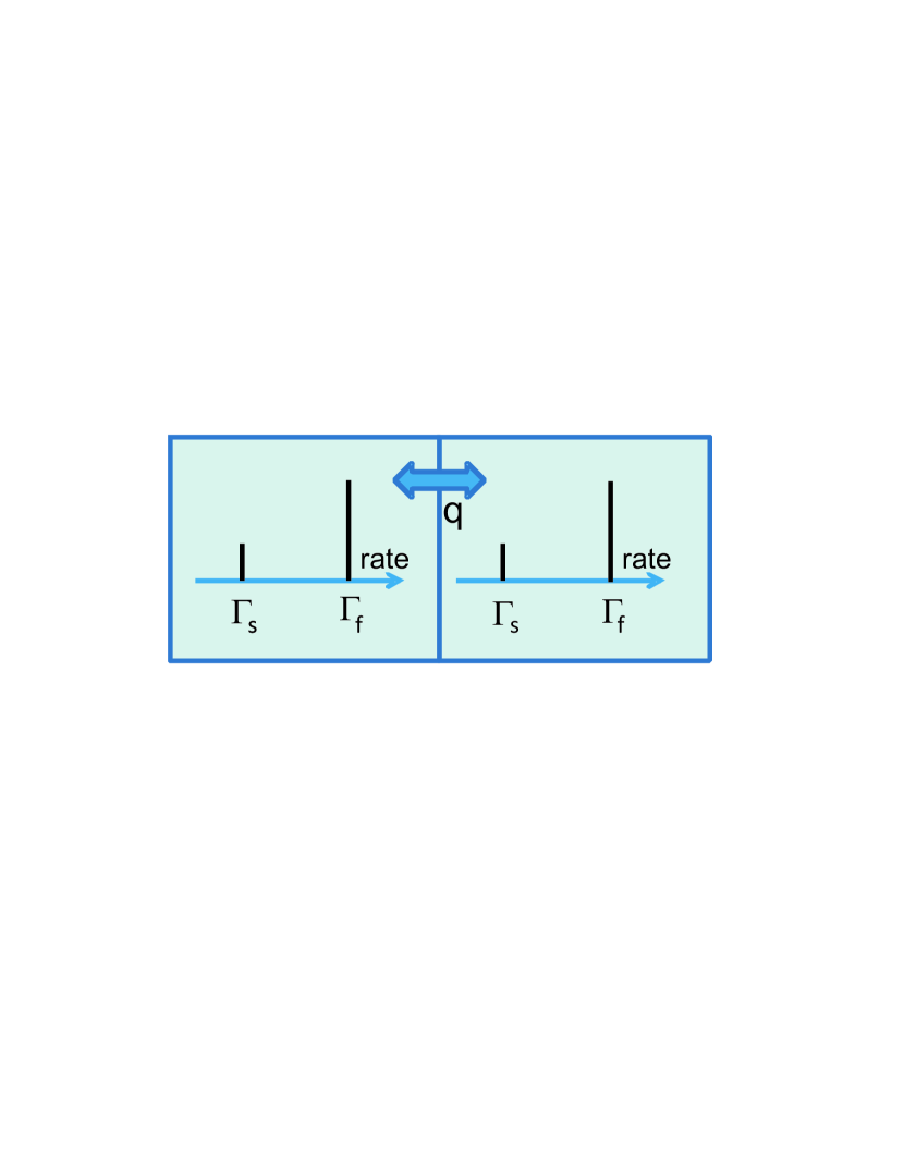
To substantiate the findings, related to the coupling effect, we analyze a minimum model which leaves the thermodynamics as well as the diffusivity unchanged upon coupling. It consists of two subsystems with a coupling constant , characterizing the strength of the coupling. The model is sketched in Fig.S1. The elementary subsystem contains two states. The slow escape rate from the lower state is , the faster escape rate from the upper state is . The relevance of dynamical heterogeneities is characterized by . The degeneracy of the high-energy state is proportional to , that of the lower state to (). The Boltzmann probabilities are proportional to . For reasons of simplicity we choose which implies . For this subsystem one directly obtains and ). Now we consider a larger system, containing two of these subsystems which are dynamically coupled. A relaxation of, e.g., subsystem 1 has two consequences. First, subsystem 1 acquires a randomly new chosen state with probability . This condition just reflects the independence of two subsequent states, populated by subsystem 1. Second, with probability subsystem 2 randomly chooses a state with probability whereas with probability no change occurs. The value of determines the strength of the coupling (: no coupling, maximum coupling). This procedure guarantees that the Boltzmann distribution in one subsystem and the average waiting time does not change as a consequence of the coupling to dynamical processes in the other subsystem.
In what follows we show via straightforward Monte Carlo simulations in combination with analytical expressions that (i) indeed decreases with increasing system size and that (ii) the coupling gives rise to dynamic length scales. The key observable, recorded during the Monte Carlo simulations are the different moments of the waiting time distribution of a single subsystem. is defined as where denotes the probability that a subsystem does not perform a relaxation process during a time interval of length .
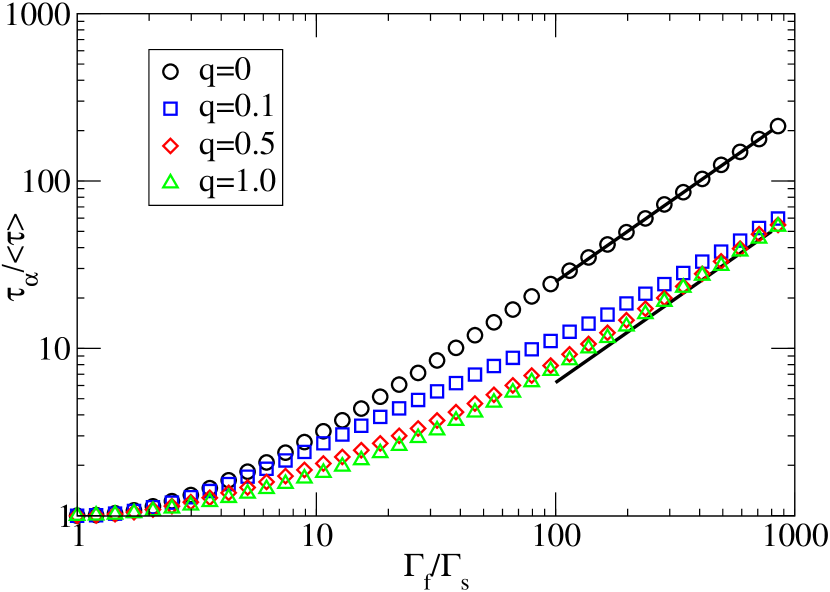
In Fig.S2 the dependence of is shown as a function of for different values of . We checked that in agreement with the setup of the model the value of does not depend on . Several interesting observations can be made. (1) decreases with increasing coupling. This naturally reflects the general system size dependencies of , reported in the main text. (2) For large dynamic heterogeneities the q-dependence disappears as long as , indicating some degree of universality for large dynamic heterogeneities. (3) In this limit one obtains for and for . These relations can be easily rationalized. For and the relevant long-time decay of is given by , implying . Together with the observed relation immediately follows. For a slow relaxation process is only observed if for both subsystems are in the slow state. If we define as the probability that none of the systems has performed a relaxation process until time one naturally has . The prefactor expresses the fact that only in one out of four cases both subsystems are initially slow. After the relaxation of, e.g., subsystem 1 and as a consequence of subsystem 1 will typically become fast afterwards. The large number of subsequent relaxation processes will for finally give rise to an exchange of the slow to the fast state in subsystem 2. Thus, for the time difference between the initial relaxation process in subsystem 1 and the first relaxation process in subsystem 2 is much smaller than . As a consequence one has , yielding as indeed observed.
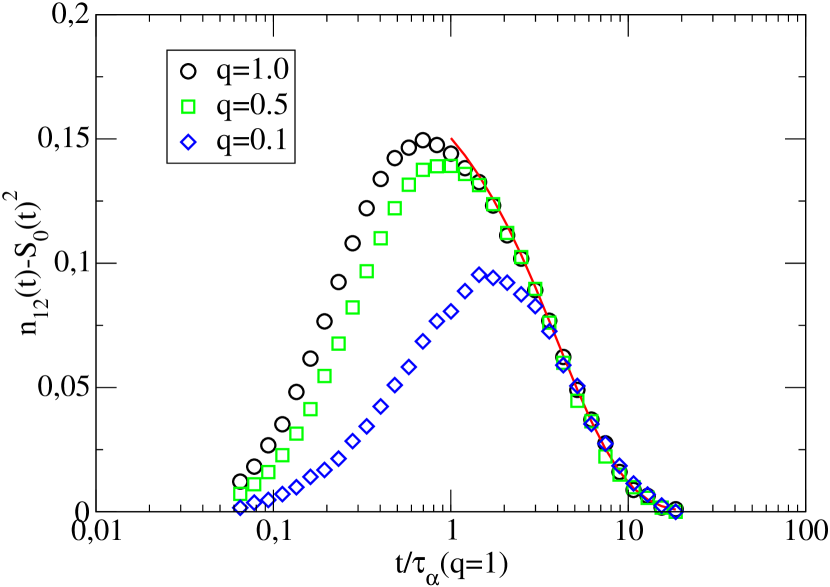
At a particular time the rates in both subsystems are uncorrelated to each other. However, for both subsystems are dynamically correlated if observed for a finite time interval; see Fig.S3. In agreement with typical data for glass-forming systems one observes a maximum correlation for . In analogy to above one expects for that which agrees with the numerical data.
Finite-size effects for small coupling constant
In generalization to above we consider two subsystems with a general distribution of rates . For one tagged system we write for the relaxation function (in discrete notation) where denotes the probability that the system is in the initial state and the probability that the system in this state has not relaxed until time . For an uncoupled system and the presence of simple rate processes one has . Since the thermodynamics does not change upon coupling the values of the remain the same. Furthermore, we define and . The index 0 always denotes the uncoupled case. Note that .
For general one has to keep track of pairs of adjacent states (see above). However, a dramatic simplification is possible in the limit of small . Restricting oneself to the lowest order effect of the coupling one can systematically neglect the forward-backward reactions which are at least of order . Thus, one can employ a mean-field type approach where a tagged system experiences fluctuations which are uncorrelated to the resulting passive exchange processes. These fluctuations induce a reorganization of the tagged system with probability per relaxation process (more specifically: MB transition). As a consequence the rate of change is . Formally, this can be written as Heuer (2008)
| (6) |
Whereas the first term on the right hand side describes the active relaxation of the tagged subsystem, starting in state , the second term characterizes a passive exchange process from some state ( to state due to the coupling to the adjacent subsystem. Since we aim to keep the dependence on only up to linear order, we can substitute by . Then integration yields
| (7) |
Thus, one can write
| (8) |
Multiplication with and summation over all states yields
| (9) |
Note that is identical to . It is exactly the first term in the brackets which in Rubner and Heuer (2008) has been denoted as and is a measure for the non-exponentiality of the total relaxation, i.e. of the dynamic heteterogeneities. Thus, we can rewrite
| (10) |
More generally, in lowest order of the tagged system of particles will experience a coupling to the surrounding particles which is proportional to the number of particles, i.e. . Furthermore, after identification of with one may finally write for to lowest order in
| (11) |
Thus, after determination of and this relation can be used to extract the dimensionless coupling constant .
Note that this estimation breaks down if (i) the second term on the right hand side approaches one (then higher-order terms of matter) or (ii) starts to be much larger than . Then the coupling is no longer proportional to because the variation of distances between different subsystems starts to matter.