Distance determination for RAVE stars using stellar models

Abstract

Aims. We develop a method for deriving distances from spectroscopic data and obtaining full 6D phase-space coordinates for the RAVE survey’s second data release.

Methods. We used stellar models combined with atmospheric properties from RAVE (effective temperature, surface gravity and metallicity) and ${(J-K_{s})}$ photometry from archival sources to derive absolute magnitudes. In combination with apparent magnitudes, sky coordinates, proper motions from a variety of sources and radial velocities from RAVE, we are able to derive the full 6D phase-space coordinates for a large sample of RAVE stars. This method is tested with artificial data, Hipparcos trigonometric parallaxes and observations of the open cluster M67.

Results. When we applied our method to a set of $16\,146$ stars, we found that 25% ($4\,037$) of the stars have relative (statistical) distance errors of $<35$%, while 50% ($8\,073$) and 75% ($12\,110$) have relative (statistical) errors smaller than 45% and 50%, respectively. Our various tests show that we can reliably estimate distances for main-sequence stars, but there is an indication of potential systematic problems with giant stars owing to uncertainties in the underlying stellar models. For the main-sequence star sample (defined as those with $\log(g){}>4$), 25% ($1\,744$) have relative distance errors $<31\%$, while 50% ($3\,488$) and 75% ($5\,231$) have relative errors smaller than 36% and 42%, respectively. Our full dataset shows the expected decrease in the metallicity of stars as a function of distance from the Galactic plane. The known kinematic substructures in the $U$ and $V$ velocity components of nearby dwarf stars are apparent in our dataset, confirming the accuracy of our data and the reliability of our technique. We provide independent measurements of the orientation of the $UV$ velocity ellipsoid and of the solar motion, and they are in very good agreement with previous work.

Conclusions. The distance catalogue for the RAVE second data release is available at http://www.astro.rug.nl/$\sim$rave, and will be updated in the future to include new data releases.

1 Introduction

The spatial and kinematic distributions of stars in our Galaxy contain a wealth of information about its current properties, its history and evolution. This phase-space distribution is a crucial ingredient if we are to build and test dynamical models of the Milky Way (e.g. Binney 2005, and references therein). More directly, the kinematics of halo stars can be used to trace the Galaxy’s accretion history (Helmi & White 1999), as has been shown to good effect in many subsequent studies (e.g. Helmi et al. 1999; Kepley et al. 2007; Smith et al. 2009). There is also much to learn from the phase-space structure of the disk, where it is possible to identify substructures due to both accretion events and dynamical resonances (e.g. Dehnen 2000; Famaey et al. 2005; Helmi et al. 2006) or learn about the mixing processes that influence the chemical evolution of the disk (e.g. Roškar et al. 2008; Schönrich & Binney 2009).

To fully exploit this rich resource, we need to analyse the full six-dimensional phase-space distribution, which clearly cannot be done without a reliable estimate of the distances to the stars under consideration. Therefore obtaining accurate distances and velocities for a representative sample of stars in our Galaxy will be essential if we are to understand both the structure of our own Galaxy and galaxy formation in general.

The most dramatic recent development in this field was the Hipparcos satellite mission (ESA 1997; Høg et al. 2000), which carried out an astrometric survey of stars down to $V\sim 12$ mag with accuracies of up to 1 mas. This catalogue enabled the distances of $\sim 10,000$ stars to be measured using the trigonometric parallax technique, with parallax errors of less than 5% (van Leeuwen 2007a, b). However, in general the resulting parallaxes only probe out to a couple of hundred parsec and are limited to the brightest stars.

This limitation of the trigonometric parallax method led researchers to attempt other techniques for calculating distances. One promising avenue is the study of pulsating variable stars, such as RR Lyraes or Cepheids, for which it is possible to accurately determine distances using period-luminosity relations (see, for example, the reviews of Gautschy & Saio 1995, 1996). These have been used effectively to probe the structure of our Galaxy, in particular the study of the old and relatively metal-poor RR Lyrae stars (Vivas et al. 2001; Kunder & Chaboyer 2008; Watkins et al. 2009).

Although pulsating variables can provide accurate tracer populations, the numbers of such stars is clearly limited; ideally we would like to determine distances for large numbers of stars and not just specific populations. As a consequence there have been numerous studies utilising photometric distance determinations, where one estimates the absolute magnitude of a star from its colour. The efficacy of this method can be seen from the work of Siegel et al. (2002) and Jurić et al. (2008), who both used this technique to model the stellar density distribution of the Galaxy. Another striking example of the power of this technique was presented by Belokurov et al. (2006), where halo turn-off stars were used to illuminate a host of substructures in the Galactic halo.

The strength of photometric distances is that they can be constructed for a wide range of stellar populations. An important recent study was carried out by Ivezić et al. (2008). In this work they took high-precision multi-band optical photometry from the Sloan Digital Sky Survey (SDSS; Abazajian et al. 2009) and constructed a photometric distance relation for F- and G-type dwarfs, using colours to identify main-sequence stars and estimate metallicity. Globular clusters were used to calibrate their photometric relation, resulting in distance estimates accurate to $\sim 15$ per cent. This is only possible due to the extremely well-calibrated SDSS photometry and, in any case, is only applicable to F- and G-type dwarfs. To determine distances for entire surveys (with a wide range of different stellar classes and populations) requires complex multi-dimensional algorithms. In this paper we develop such a technique to estimate distances for stars using photometry in combination with stellar atmosphere parameters derived from spectra.

One of the motivations behind our study is so that we can complement the Radial Velocity Experiment (RAVE Steinmetz et al. 2006; Zwitter et al. 2008). This project, which started in 2003, is currently measuring radial velocities and stellar atmosphere parameters (temperature, metallicity and surface gravity) for stars in the magnitude range 9 $<$ $I$ $<$ 12. By the time it reaches completion in $\sim 2011$ it is hoped that RAVE will have observed up to one million stars, providing a dataset that will be of great importance for Galaxy structure studies. A number of publications have already made use of this dataset (e.g. Smith et al. 2007; Klement et al. 2008; Munari et al. 2008; Siebert et al. 2008; Veltz et al. 2008), but to fully utilise the kinematic information we crucially need to know the distances to the stars. Unfortunately, most of the stars in the RAVE catalogue are too faint to have accurate trigonometric parallaxes, hence the importance of a reliable and well-tested photometric/spectroscopic parallax algorithm. When distances are combined with archival proper motions and high precision radial velocities from RAVE, this dataset will provide the full 6D phase-space coordinates for each star. Clearly such an algorithm for estimating distances will be a vital tool when carrying out kinematic analyses of large samples of Galactic stars, not just for the RAVE survey but for any similar study.

The future prospects for distance determinations are very promising. In the next decade the Gaia satellite (Perryman et al. 2001) will observe up to $10^{9}$ stars with exquisite astrometric precision. The mission is due to start in 2012, but a final data release will not arrive until near the end of the decade at the earliest. Furthermore, as with any such magnitude limited survey, there will be a significant proportion of stars for which their distances are too great for accurate trigonometric parallaxes to be determined. Therefore, although Gaia will revolutionise this field, it will not close the chapter on distance determinations for stars in the Milky Way and so photometric parallax techniques will remain of crucial importance.

In this paper we present our algorithm for determining distances, which we construct using stellar models. When we apply this method to the RAVE dataset we are able to reproduce several known characteristics of the kinematics of stars in the solar neighbourhood. In §2, we present a general introduction. We discuss the connection between stellar evolution theory, stellar tracks and isochrones to gain insight in these topics before presenting our statistical methods for the distance determination and testing the method using synthetic data. In §3 we apply the method to the RAVE dataset and compare the distances to external determinations, namely stars in the open cluster M67 and nearby stars with trigonometric parallaxes from Hipparcos. Results obtained from the phase-space distribution are presented in §4 to check whether the data reflect known properties of our Galaxy. We present a discussion of the uncertainties and limitations of the method in §5 and conclude with §6.

2 Method for distance determination

2.1 Stellar models and observables

Stellar models are commonly used to estimate distances, for instance in main-sequence fitting. Such methods work for collections of stars, but models can also be used to infer properties of individual stars, such as ages (Pont & Eyer 2004; Jorgensen & Lindegren 2005; da Silva et al. 2006). In our analysis we utilise this approach, combining stellar parameters (temperature, metallicity and surface gravity) with photometry to estimate a star’s absolute magnitude.

The evolution of a star is fully determined by its mass and initial chemical composition (e.g. Salaris & Cassisi 2005). Stellar tracks and isochrones can be seen (in a mathematical sense) as a function ($\mathcal{F}$) of alpha-enhancement ([$\alpha$/Fe]), metallicity ($Z$), mass ($m$) and age ($\tau$) that maps onto the observables: absolute magnitude (${M_{\lambda}}$), surface gravity ($\log(g)$), effective temperature ($T_{\text{eff}}$), and colours, i.e.

$$\begin{array}[]{ll}&\mathcal{F}({[\alpha\text{/Fe}]},Z,\tau,m)\mapsto({M_{\lambda}},\log(g),T_{\text{eff}},\text{colours,\ldots}).\\ \end{array}$$ (1)

In particular, an isochrone is the function $\mathcal{I}(m)$ of mass, which is obtained from $\mathcal{F}$ by keeping all other variables constant.

Assuming solar $\alpha$-abundance, ${[\alpha\text{/Fe}]}$= 0, we define the function $\mathcal{F}_{0}(Z,\tau,m)$, which is $\mathcal{F}$ with ${[\alpha\text{/Fe}]}$ fixed at 0,

$$\begin{array}[]{lll}\mathcal{F}_{0}(Z,\tau,m)&=&\mathcal{F}(Z,\tau,m)|_{{[\alpha\text{/Fe}]}=0}\\ &\mapsto&({M_{\lambda}},\log(g),T_{\text{eff}},{\rm colours}...).\\ \end{array}$$ (2)

Therefore the isochrones or stellar tracks from a given model can be seen as samples from the theoretical stars defined by $\mathcal{F}_{0}(Z,\tau,m)$. Throughout this paper we assume solar-scaled metallicities, which means that ${[\alpha\text{/Fe}]}=0$ and ${\text{[M/H]}}={\text{[Fe/H]}}$, where [M/H] is defined as $\log(Z/Z_{\odot})$.

For our study we use the $Y^{2}$ (Yonsei-Yale) models (Demarque et al. 2004). These models can be downloaded from the $Y^{2}$ website, where also an interpolation routine is available, called YYmix2. It should be noted that these models ignore any element diffusion that may take place in the stellar atmosphere (see, for example, Tomasella et al. 2008).

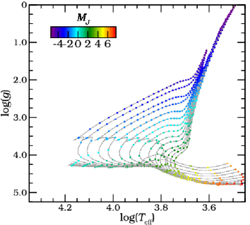
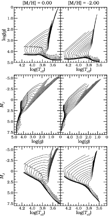
A sample of theoretical ‘model stars’ from these $Y^{2}$ models are shown in Fig. 1. Each model star is represented as a dot and the connecting lines correspond to the isochrones of different ages. In Fig. 2 we show the same isochrones as Fig. 1, illustrating the relation between $M_{J}$ and $T_{\text{eff}}$, and between $M_{J}$ and $\log(g)$ separately. Clearly, for a given $T_{\text{eff}}$, $\log(g)$ and [M/H] it is not possible to infer a unique $M_{J}$ (i.e. the function $\mathcal{F}_{0}$ is not injective). This can be seen most clearly in Fig. 1, where around $\log(T_{\text{eff}})$ = 3.8, $\log(g)$ = 4 the isochrones overlap. However, this is also evident in other regions; for example in the top panels of Fig. 2 the isochrones are systematically shifted as metallicity goes from 0 to $-2$. Because we are unable to determine a unique $M_{J}$ for a given star we are forced to adopt a statistical approach, i.e. obtaining a probability distribution for $M_{J}$.

From Fig. 2 we can see how errors in the observables $\log(g)$ and $T_{\text{eff}}$ affect the uncertainty in the absolute magnitude ($M_{J}$ in this example). The middle row in Fig. 2 shows that the value of $M_{J}$ is better defined by $\log(g)$ for red giant branch (RGB) stars than for main-sequence stars, independently of their metallicity. On the other hand, the bottom row of Fig. 2 shows that $T_{\text{eff}}$ essentially determines $M_{J}$ for main-sequence stars, again independently of metallicity. We therefore expect that a small error in $\log(g)$ will give better absolute magnitude estimates for RGB stars, while a small error in $T_{\text{eff}}$ will have a similar effect on main-sequence stars. We also expect this not to be strongly dependent on metallicity.

Figure 1: $\log(g)$ versus $\log(T_{\text{eff}})$ plot for isochrones from 0.01-15 Gyr spaced logarithmically, for [M/H] = 0 and ${[\alpha\text{/Fe}]}$ = 0. Colour indicates the absolute magnitude in the $J$ band.

Figure 2: Isochrones for ${[\alpha\text{/Fe}]}$ = 0, [M/H] = 0 (left column) and [M/H] = $-2$ (right column), ages ranging from 0.01-15 Gyr spaced logarithmically. The dashed line indicates the youngest (0.01 Gyr) isochrone. Top row: Similar to Fig. 1, shown for completeness. Middle row: $M_{J}$ is best restricted by $\log(g)$ for RGB stars. Bottom row: $M_{J}$ is best restricted by $T_{\text{eff}}$ for main-sequence stars.

2.2 Description of the method

We now outline the method that we use to estimate the probability distribution function (PDF) for the absolute magnitude (or, equivalently, the distance). Previous studies have employed similar techniques to determine properties of stars using stellar models. A selection of such work can be found in the following references: Pont & Eyer (2004); Jorgensen & Lindegren (2005); da Silva et al. (2006).

Our method requires a set of model stars. As was discussed in §2.1, we have chosen to use the $Y^{2}$ models (Demarque et al. 2004). We generate our set of isochrones using the YYmix2 interpolation code. The set consists of 600 isochrones, with 40 different ages, spaced logarithmically between 0.01 and 15.0 Gyr, and 15 different metallicities with 0.25 dex separation (corresponding to 1 sigma in [M/H] for the RAVE data; see Section 3.1) between [M/H] = $-2.5$ and [M/H] = $1.0$. The separation between the points of the isochrones has been visually inspected and is, in general, smaller than the errors in $T_{\text{eff}}$ and $\log(g)$. These isochrones do not track the evolution beyond the RGB tip. We only use the isochrones with ${[\alpha\text{/Fe}]}$ = 0 because our observational data do not allow an accurate measurement of ${[\alpha\text{/Fe}]}$ and for most of our stars we expect ${[\alpha\text{/Fe}]}\approx 0$. Later, in §2.3, we show that assuming ${[\alpha\text{/Fe}]}=0$ for stars having ${[\alpha\text{/Fe}]}>0$ does not introduce any noticeable bias in our results.

Let us suppose we have measured the following parameters for a sample of stars: $T_{\text{eff}}$, $\log(g)$, [M/H] and ${(J-K_{s})}$. Each of these quantities will have associated uncertainties due to measurement errors ($\sigma_{T_{\text{eff}}}$, $\sigma_{\log(g)}$, $\sigma_{{\text{[M/H]}}}$ and $\sigma_{{(J-K_{s})}}$), which we assume are Gaussian. For each observed star we first need to obtain the closest matching model star, which we do by minimising the usual $\chi^{2}$ statistic,

$$\chi^{2}_{\rm model}=\sum_{i=1}^{n}\frac{(A_{i}-A_{i,{\rm model}})^{2}}{\sigma_{A_{i}}^{2}},$$ (3)

where $A_{i}$ corresponds to our observable parameters (i.e. $n=4$ in this case) and $A_{i,{\rm model}}$ the corresponding parameters of the model star, as given by the set of isochrones. By minimising Eq. (3), we obtain the parameters for the most-likely model star, denoted $\overline{A_{1}},...,\overline{A_{n}}$.

Having identified the most probable model, we generate 5000 realisations of the observations that could be made of this model star by sampling Gaussian distributions in each observable that are centred on the model values, with the dispersion in each observable equal to the errors in that quantity. By drawing our realisations about $\overline{A_{i}}$ we are making the assumption that the observables are just a particular realisation of the model (e.g. chapter 15.6 of Press et al. 1992). Then for each such realisation we again find the most probable star by minimising $\chi^{2}_{\rm model}$ in Eq. (3). The final PDF is the frequency distribution of the intrinsic properties of the model stars that have been located in this way. One may argue that the first step of finding the closest model star is not formally correct since it does not have a corresponding Bayesian equivalent. However, we have found no apparent differences in the results in tests where we exclude this step in the procedure.

We use the PDF obtained from the Monte Carlo realisations to determine the distance. Due to the non-linearity of the isochrones, as can be seen in Fig. 2, we expect the PDFs to be asymmetric. In such cases the mode and the mean of the PDF are not the same. Since the mean is a linear function, we choose to calculate the mean and standard deviations of $M_{J}$ (and distance $d$) from the Monte Carlo realisations. This gives us our final determination for the distance to each star and its associated error. We also compared the method using the median of the distribution of absolute magnitudes instead of the mean, and found no significant differences.

We have not made use of any priors in this analysis. We could have invoked a prior based on, for example, the luminosity function or mass function of stars in the solar neighbourhood. However, since the luminosity function of our sample is not an unbiased selection from the true luminosity function in the RAVE magnitude range (Zwitter et al. 2008), this makes the task of quantifying our prior very difficult. We therefore choose to adopt a flat prior in order to avoid any potential biases from incorrect assumptions. However, it is hoped that by the end of the RAVE survey it will have produced a magnitude limited catalogue, at which point it may become possible to invoke a prior based on the luminosity function.

2.3 Testing the method

To test the method, we take a sample of 1075 model stars. This set is large enough for testing purposes, allowing us to determine which kind of stars the method works best for. The sample of 1075 model stars are taken from a coarsely generated grid of isochrone models with metallicity ${\text{[M/H]}}=0$. We convolve [M/H], $T_{\text{eff}}$, $\log(g)$ and the colours with Gaussians with dispersions comparable to the error in the RAVE survey in order to mimic our measurements ($\sigma_{T_{\text{eff}}}$ = 300 K, $\sigma_{\log(g)}$ = 0.3 dex, $\sigma_{{\text{[M/H]}}}$ = 0.25 dex, $\sigma_{J}\approx\sigma_{K_{s}}\approx$ 0.02 mag; see §3.1).

The reason for choosing a fixed metallicity is twofold. In §2.1 we have seen that different metallicities should give similar results in terms of the precision with which the absolute magnitude can be derived. Secondly, it also means that the results only have to be compared to one set of isochrones, making it easier to interpret. Note that although one metallicity is used to generate the sample, after error convolution, isochrones for all metallicities are used for the fitting method.

Figure 3: Effect of the uncertainties in $\log(g)$ and $T_{\text{eff}}$ on the estimated absolute magnitude $M_{J}$. The main-sequence and RGB stars perform best. Reducing the errors in $\log(g)$ has the largest effect. Left column: Errors similar to the RAVE dataset, $\sigma_{T_{\text{eff}}}$ 300 K and $\sigma_{\log(g)}$ = 0.3. Middle column: Reducing the errors in effective temperature, $\sigma_{T_{\text{eff}}}$ = 150 K. Right column: Reducing the errors in surface gravity, $\sigma_{\log(g)}$ = 0.15. Top row: The sample of 1075 stars, with colours indicating errors, clipped to a value of $\sigma_{M_{J}}$ = 1.25. Middle row: CMD with colours indicating the same errors as the top row. Bottom row: Difference between input (i.e. model) and estimated absolute magnitude versus input absolute magnitude. We include a running mean and dispersion. The colours correspond to the same scale as in the top row. The spread in this distribution grows as the estimated uncertainty in $M_{J}$ grows (as indicated by the colour change).

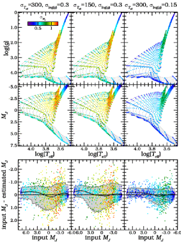
We run the method described in the previous section on this set of 1075 stars and analyse the results in the left column of Fig. 3. The colours indicate the estimated errors on $M_{J}$ obtained from our algorithm and are clipped to a value $\sigma_{M_{J}}$ = 1.25. The middle row shows the results on a colour-magnitude diagram (CMD). Stars on the main sequence and on the RGB appear to have the smallest errors as expected (see §2.1). In the bottom row, the difference between the input (i.e. model) and estimated magnitude is plotted against the input magnitude of the model star from which the estimate was derived, showing the deviation from the input absolute magnitude grows with $\sigma_{M_{J}}$, as expected. The method appears to give reasonable results, showing no serious systematic biases. The left column of Fig. 3 shows that for the main sequence and RGB stars in the RAVE data set we expect a relative distance error of the order of 25% (blue colours), and for the other stars around 50-60% (green to red colours).

We run this procedure again, now testing the effect of reducing the error in $T_{\text{eff}}$. If we decrease the error in $T_{\text{eff}}$ to 150 K, we obtain the results shown in the middle column of Fig. 3. The errors in $M_{J}$ do not seem to have changed much, except for a very slight improvement for the main-sequence stars. If, on the other hand, we decrease the error in $\log(g)$ to 0.15 dex while keeping the $T_{\text{eff}}$ error at 300 K, we obtain the results shown in the right column in Fig. 3. This shows that the accuracy and precision with which we can determine $M_{J}$ has increased significantly. Therefore, reducing the uncertainty in $\log(g)$ is much more effective than a similar reduction in $T_{\text{eff}}$ and will result in significant improvements in the estimate of the absolute magnitude. In future, high precision photometry from surveys such as Skymapper’s Southern Sky Survey (Keller et al. 2007) may aid the ability of RAVE to constrain the stellar parameters.

We carry out an additional test to quantify whether our decision to only fit to ${[\alpha\text{/Fe}]}=0$ models will bias our results. To do this we generated three similar catalogues of model stars, but with ${[\alpha\text{/Fe}]}{}=0,0.2,0.4$ dex. We then repeat the above procedure (as usual fitting to models with ${[\alpha\text{/Fe}]}$ fixed at 0) and analyse the resulting distances. Reassuringly we find that there is no difference between the accuracy of the three catalogues, justifying our decision to carry out the model fitting using only ${[\alpha\text{/Fe}]}=0$ models.

3 Application to RAVE data

3.1 Data

The Radial Velocity Experiment (RAVE) is an ongoing project measuring radial velocities and stellar atmosphere parameters (temperature, metallicity, surface gravity and rotational velocity) of up to one million stars in the Southern hemisphere. Spectra are taken using the 6dF spectrograph on the 1.2m UK Schmidt Telescope of the Anglo-Australian Observatory, with a resolution of R = 7 500, in the $8\,500-8\,750$ Å window. The input catalogue has been constructed from the Tycho-2 and SuperCOSMOS catalogues in the magnitude range $9<I<12$. To date RAVE has obtained spectra of over 250 000 stars, 50 000 of which have been presented in the most recent data release (Zwitter et al. 2008).

This second RAVE data release provides metallicity ([M/H]), $\log(g)$ and $T_{\text{eff}}$ from the spectra, and has been cross-matched with 2MASS to provide $J$ and $K_{s}$ band magnitudes. The $(JK)_{\text{ESO}}$ colours used for the $Y^{2}$ isochrones match the 2MASS $(JK_{s})_{\text{2MASS}}$ colours very well, so no colour transformation is required (Carpenter 2001).

We choose to use the $J$ and $K_{s}$ bands because they are in the infrared (IR) and are therefore less affected by dust than visual bands. To see whether extinction will be significant for our sample we carry out a simple test using the dust maps of Schlegel et al. (1998). If we model the dust as an exponential sheet with scale-height 130pc (Drimmel & Spergel 2001), we find that given the RAVE field-of-view, a typical RAVE dwarf located 250pc away would suffer $\sim$0.03 mag of extinction in the $J$-band. This corresponds to a distance error of $\sim 1\%$, which is negligible compared to the overall uncertainty inherent in our method. Reddening is similarly unimportant, with the same typical RAVE star suffering $\sim$0.02 mag reddening in ${(J-K_{s})}$. Even if we only consider fields-of-view with $\left|b\right|<40^{\circ}$ then we find that the extinction for a star at a distance of 250pc is only 0.04 mag (with corresponding distance error of $\sim 2\%$). Note that for future RAVE data releases it may be possible to use information from the spectra to include extinction corrections for some individual stars (Munari et al. 2008).

The observed parameter values used for the model fitting routine are the weighted average of the available values, where the weight is the reciprocal of the measurement error:

$$X_{\rm weighted}=\frac{\sum_{j}w_{j}X_{j}}{\sum_{j}w_{j}},$$ (4)

where $X_{j}$ are the measured values and $w_{j}=1/\sigma_{j}^{2}$ the corresponding weight. The error in the average is calculated as:

$$\sigma_{\rm weighted}^{2}=\frac{1}{\sum_{j}1/\sigma_{j}^{2}}.$$ (5)

For the RAVE data, $T_{\text{eff}}$ is determined only from the spectra, i.e. not photometrically, which means that $T_{\text{eff}}$ and ${(J-K_{s})}$ are uncorrelated in the sense that they are independently observed. Therefore we can use both $T_{\text{eff}}$ and ${(J-K_{s})}$ in Eq. 3 to obtain our distance estimate. The error in ${(J-K_{s})}$ is small compared to other colours, which means that adding further colours will result in only a negligible improvement on the uncertainty of the absolute magnitude. For this reason we only use this one colour.

The current RAVE data release (Zwitter et al. 2008) does not include individual errors for each star’s derived parameters and so for the errors in [M/H], $T_{\text{eff}}$ and $\log(g)$ we take 0.25 dex, 300 K and 0.3 dex respectively. The errors in [M/H] and $T_{\text{eff}}$ are reasonable averages for different types of stars of low temperature, as can be seen from Fig. 19 in Zwitter et al. (2008). Even though our $\log(g)$ error estimate is slightly smaller compared to this figure, our results do not show evidence of an underestimation in the distance errors (§3.3.1). In fact, repeated observations of certain stars in the RAVE catalogue indicate that these errors may be conservative (Steinmetz et al. 2008). The RAVE DR2 dataset has two metal abundances, one uncalibrated, determined from the spectra alone ([m/H]), and a calibrated value ([M/H]). The latter is calibrated using a subset of stars with accurate metallicity estimates and it is this value which we use in the fitting method. As above we assume solar-scaled metallicities, which means that ${[\alpha\text{/Fe}]}=0$ and ${\text{[M/H]}}={\text{[Fe/H]}}$.

3.2 Determining distances to RAVE stars

We now use the data set described above to derive absolute magnitudes using our model fitting method (see §2.2).

The RAVE second data release (Zwitter et al. 2008) contains 51 829 observations, of which 22 407 have astrophysical parameters. We first clean up the dataset by requiring that the stars have all parameters required by the fitting method ([M/H], $\log(g)$, $T_{\text{eff}}$, $J$, $K_{s}$), a signal to noise ratio S2N $>$ 20, no 2MASS photometric quality flags raised (i.e. we require ‘AAA’) and the spectrum quality flag to be empty to be sure we have no obvious binaries or cosmic ray problems. Although this latter flag will eliminate clear spectroscopic binaries (132 individual stars, 0.2%), our sample must suffer from binary contamination given the estimated $37\%$ binary fraction for F and G stars in the Copenhagen-Geneva survey (Holmberg et al. 2009) or the much lower estimates $6$-$14$% of Famaey et al. (2005). In future the use of repeated observations for the RAVE sample will give a better understanding of the effect of binaries on, for instance, the T${}_{\text{eff}}$ and $\log(g)$ estimates (Matijevic et al. 2009, in prep.).

Although most of the RAVE survey stars in this data release are located at high latitude (with $|b|>25^{\circ}$), there are a limited number of calibration fields with $|b|<10^{\circ}$. We remove these low-latitude fields from our analysis since they could suffer from significant extinction which will bias our distance estimates.

For some stars multiple observations are available, these are grouped by their ID, and a weighted average (Eq. 4) and corresponding error (Eq. 5) for all radial velocities are calculated. The astrophysical parameters ([M/H], $\log(g)$ and $T_{\text{eff}}$) have nominal errors as described in §3.1. For these parameters an unweighted average is calculated but the error in the average is kept equal to the nominal error. The total number of independent sources matching these constraints is 16 645.

Once we have our clean sample of stars we first find the best model star as described in §2.1. If it has a $\chi^{2}_{\rm model}\geq 6$ (Eq. 3) it is not considered further. This last step gets rid of the $\sim 3\%$ of stars that are not well fit by any model.

Our final sample has 16 146 sources which are used for the model fitting method to obtain an estimate of the distance and associated uncertainty for each star.

Figure 4: Error distribution (left) and cumulative plot (right) for $M_{J}$ (top) and distance (bottom). These distributions are for the clean sample of 16 146 stars (see §3.2). The black line includes all the stars, while the grey line shows the distribution for main-sequence stars (defined here as those with $\log(g){}>4$).

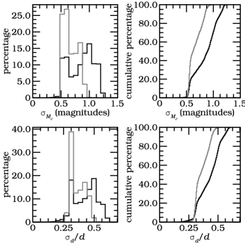
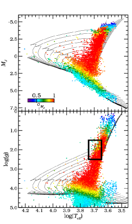
The distribution of uncertainties in the absolute magnitude and the distance for this clean sample of 16 146 stars can be found in Fig. 4 (black line). The $x$-axes are scaled such that the uncertainties can be compared using $\sigma_{d}/d\approx\sigma_{M_{J}}\ln(10)/5=0.46\sigma_{M_{J}}$. The differences between the two histograms show that the error in the apparent $J$ magnitude does contribute to the relative distance error. In Fig. 5 we show how the uncertainties behave for the different types of stars. The distribution of uncertainties for the sample is as follows: 25% ($4\,037$) of the stars have relative (statistical) distance errors of $<35$%, while 50% ($8\,073$) and 75% ($12\,110$) have relative (statistical) errors smaller than 45% and 50% respectively. For main-sequence stars (which we define here as those with $\log(g){}>4$, the grey line in Fig. 4) the distribution of uncertainties is: 25% ($1\,744$) have relative distance errors $<31\%$, while 50% ($3\,488$) and 75% ($5\,231$) have relative errors smaller than 36% and 42% respectively.

The $Y^{2}$ isochrones do not model the later evolutionary stages of stars, such as the horizontal branches and the asymptotic giant branch. The red clump (RC), which is the horizontal branch for Population I stars, is a well populated region in the CMD due to the relatively long lifetime of this phase ($\sim 0.1$ Gyr) (Girardi et al. 1998). Therefore we expect the RAVE sample to include a non negligible fraction of RC stars. Using the selection criteria of Veltz et al. (2008) and Siebert et al. (2008), namely $0.5<{(J-K_{s})}<0.7$ and $1.5<\log(g)<2.5$ we find about $\sim 10$% of the RAVE sample could be on the RC. This region is highlighted in Fig 5 with a black rectangle. The distance to many of these stars can be determined using the almost constant absolute magnitude of the RC (e.g. Veltz et al. 2008; Siebert et al. 2008). However, since there may be better ways to isolate the RC region, we choose to determine the distances for all these stars using our method. Therefore, in the rest of this paper we make no distinction between RC and RGB stars. Nonetheless, we recommend users to discard what they believe may be RC stars, and possibly to determine their distances using the absolute magnitude of the RC.

Figure 5: Results after applying the model fitting method to the RAVE data. Colours indicate the magnitude of the error in $M_{J}$. Only stars with $\sigma_{M_{J}}<1.0$ are plotted. Isochrones for [M/H] = 0 are plotted for comparison. Top: CMD of RAVE dataset showing that the stars on the main sequence and RGB stars have the smallest errors. Bottom: $\log(T_{\text{eff}})$ versus $\log(g)$, colour coding as in the top panel. The black rectangle approximately highlights the area in which red clump (RC) stars are expected to be found. The assumed error in $\log(g)$ is 0.3 dex and in $T_{\text{eff}}$ is 300 K. Note that although the RGB stars in this panel do not match the [M/H] = 0 isochrones, they are more consistent with the isochrones corresponding to their measured metallicities.

3.3 Testing of RAVE distances

In order to verify the accuracy of our distance estimates, we perform two additional checks using external data and observations of the open cluster M67.

3.3.1 Hipparcos

The best way to assess our distance estimates is through independent measurements. For calibration purposes a number of RAVE targets were chosen to be stars previously observed by the Hipparcos mission, which means that for these stars we will have an independent distance determination from the trigonometric parallax. These stars are at the brighter end of the RAVE magnitude range and are mostly dwarfs.

We take the reduction of the Hipparcos data as presented by van Leeuwen (2007a, b) and cross-match these with our RAVE stars. In order to maximise the number of RAVE stars we use a preliminary dataset larger than the public release described in §3.1; this dataset contains $\sim 250\,000$ stars, but has not undergone the rigourous verification and cleaning of the public data release. This cross-matching provides 624 stars for which the Hipparcos parallax errors are less than 20% and our distance errors are less than 50%. Note that when dealing with uncertain trigonometric parallaxes it is well known that the corresponding distance determinations are systematically underestimated (Lutz & Kelker 1973). We correct for this using the prescription described in section 3.6.2 of Binney & Merrifield (1998), in particular equation (3.51).

Figure 6: Bottom: Distance from our method versus Hipparcos distance, the dashed line corresponds to equal distances. Top: Histogram of relative distance differences between our distance and that of Hipparcos. The dashed line shows the expected distribution given the quoted errors from our method and Hipparcos. Note that the observed distribution is narrower, indicating that our errors are probably overestimated for these stars (see §3.3.1).

Figure 7: Relative offset in distance from our method vs the trigonometric parallax determination from Hipparcos, as function of $\log(g)$, [M/H], $(J-K_{s})$ and $T_{\text{eff}}$. We include a running mean and dispersion.

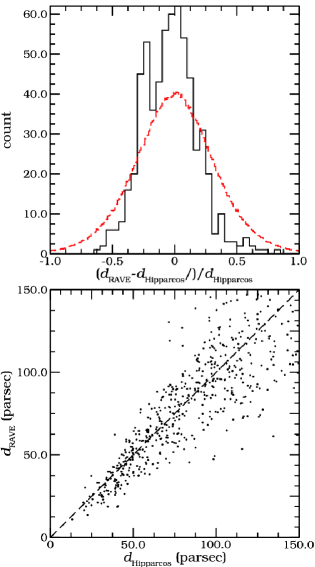
In the bottom panel of Fig. 6 we show a plot of our distance estimate ($d_{\text{RAVE}}$) vs the Hipparcos distance ($d_{\text{Hipparcos}}$). Clearly there is some scatter in this distribution, but in the top panel we quantify this by showing the distribution of $(d_{\text{RAVE}}-d_{\text{Hipparcos}})/d_{\text{Hipparcos}}$. The curve shows the expected distribution given our error on $d_{\text{RAVE}}$ and approximating the error on $d_{\text{Hipparcos}}$ from the error on the parallax (the true error on $d_{\text{Hipparcos}}$ is non-trivial to calculate owing to the aforementioned Lutz-Kelker bias). It can be seen that the predicted distribution is broader than the observed one; if we assume our estimate of the Hipparcos errors are reasonable, this discrepancy between the two distributions indicates that our errors are probably overestimated. We believe this can be explained by the fact that only the brightest RAVE stars have trigonometric parallaxes in the Hipparcos catalogue. These brighter stars have higher S2N than the average RAVE stars and so the true uncertainties on the stellar parameters are actually smaller than our adopted values. The average S2N for these 624 stars is $\sim$64, which is twice the typical S2N ratio for RAVE stars; correspondingly the uncertainties on the stellar parameters will be smaller by a factor of 1.3 (section 4.2.4 of Zwitter et al. 2008).

We can quantify the overestimation in our distance errors for these stars. The $3\sigma$ clipped standard deviation of the observed distribution is 22.1% and that of the predicted distribution is 27.8%. To give the predicted distribution the same spread as the observed distribution would require us to decrease the distance errors from our method for these stars by $\sim$35%. Note that the $3\sigma$ clipping of this distribution is necessary since a small fraction of our distances are in significant disagreement with Hipparcos. Of the 624 stars in this cross-matched sample, there are 3 with distance overestimates of more than 50%, however closer inspection shows they qualify to be RC stars (§3.2). One more star qualifies as RC star and has a distance overestimate of 40%, and one star with a $\log(g)=2.8$ has a distance overestimate of 20%. The systematic overestimation for possible RC stars and RGB stars is in agreement with our findings in the next section.

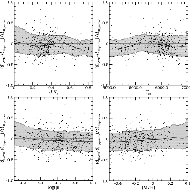
In Fig. 7 we show the distribution of $(d_{\text{RAVE}}-d_{\text{Hipparcos}})/d_{\text{Hipparcos}}$ as a function of the 2MASS colour ${(J-K_{s})}$ and of the three main stellar parameters ($T_{\text{eff}}$, [M/H], $\log(g)$). We see no clear systematic trends at a level of more than $\sim 15\%$ in any of the properties shown here, which implies that our method is producing reliable distances for main-sequence stars.

3.3.2 M67 giants

Figure 8: Bottom: CMD of M67 giants on top of theoretical solar-metallicity $Y^{2}$ isochrones, with the 4 Gyr isochrone in black. The isochrones are spaced logarithmically in age between 0.01 to 15 Gyr. Horizontal lines indicate 1$\sigma$ uncertainties in $(J-K_{s})$ and the uncertainties in the vertical direction are smaller than the size of the data-point. Top: Similar to top panel, except now for $\log(g)$ versus $\log(T_{\text{eff}})$.

The results from the previous section give us confidence the method works well for nearby main-sequence stars, but give us no indication of the validity of the distances to giant stars.

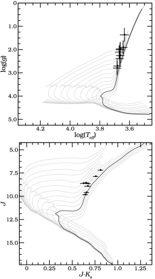
Our preliminary RAVE dataset includes a small number of RGB stars which are members of the old open cluster M67. As the distance to M67 is relatively well known, this makes a perfect test case for these stars. M67 has a distance modulus of $(m-M)_{V}=9.70$, near-solar metallicities and an age of $\tau\approx 4$ Gyr (VandenBerg et al. 2007).

We identify members of M67 using the following criteria: offset from the cluster centre of less than 0.55°; heliocentric radial velocity within 3.3 ${\rm km\,s}^{-1}$ of the mean value of 32.3 ${\rm km\,s}^{-1}$ (Kharchenko et al. 2005), where this value of 3.3 ${\rm km\,s}^{-1}$ corresponds to three times the uncertainty in the mean velocity; signal to noise ratio S2N $>$ 20; $\log(g)<3.5$. A total of 8 stars pass these criteria. In Fig. 8 we show these members, where one star is observed twice. For these stars our method gives a distance of $\sim$1.82$\pm$0.27 kpc, more than twice the distance from the literature ($\sim 0.8$ kpc; VandenBerg et al. 2007). Note however that the 4 stars at $J\approx 8.8$ qualify as RC stars as defined in §3.2. If we exclude these stars then the distance to M67 is $1.48\pm 0.36$ kpc. The distance estimate is now within 2 sigma of the assumed real distance of 0.8 kpc, but still systematically overestimated. This overestimation can be understood when one considers the performance of the stellar models. In the bottom panel we show the CMD of the members with a set of isochrones for comparison. The black isochrone is for an age similar to that of the M67 population ($4$ Gyr) and of solar metallicity. At least one or both of the predicted colour and absolute magnitude of the stars is incorrect. In the top panel we show a plot of $\log(g)$ vs. $T_{\rm eff}$, which shows that the stars do not lie on the isochrone in this plane either. Although the stars are within 1 or 2$\sigma$ from the $4$ Gyr isochrone, the deviation is systematic, particularly for the brighter RGB stars. This discrepancy will clearly impair our method and hence it is not surprising that our distances are affected. The difficulty of obtaining isochrones that match giants is a long standing problem that is being addressed by various authors (e.g. VandenBerg et al. 2008; Yadav et al. 2008).

Therefore, given the limitations of the models used in this work, our distances for stars with $\log(g)<3$ should be treated with caution. They can still be useful for analysing trends in the data (§4), but distances to individual stars are likely to be inaccurate. Note as well that our simplification to treat RC as RGB stars will lead to an overestimation of their distance. We return to the issue of stellar models in the discussion (§5.1).

3.4 6D phase-space coordinates for stars in the RAVE dataset

Figure 9: Distribution of uncertainties for velocity components $U$ (solid line), $V$ (dashed line) and $W$ (dotted line) velocities. This corresponds to the clean sample of 16 146 stars (see §3.2). The black line includes all the stars, while the grey line shows the distribution for main-sequence stars (defined here as those with $\log(g){}>4$).

Besides providing distances to RAVE stars, we also provide full 6D phase-space information derived using the radial velocities (from RAVE) and the archival proper motions contained in the RAVE catalogue (from the Starnet2, Tycho2, and UCAC2 catalogues; see Zwitter et al. 2008).

We use the Monte Carlo techniques described above to calculate 6D phase-space coordinates assuming Gaussian errors on the observed quantities (radial velocities, proper motions, etc). This is done using the transformations given by Johnson & Soderblom (1987).

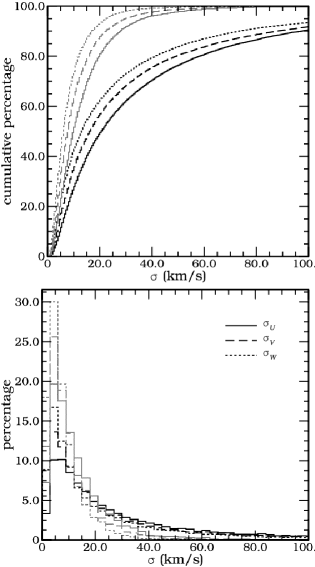
The coordinate system we use is a right-handed Cartesian coordinate system centred on the Galactic Centre (GC): the $x$ axis is aligned with the GC-Sun axis with the Sun located at $x=-8$ kpc; the $y$ axis pointing in the direction of rotation and the $z$ axis pointing towards the Northern Galactic Pole (NGP). The velocities with respect to the Sun in the directions of $(x,\,y,\,z)$ are ($U,\,V,\,W$) respectively, with the rest frame taken at the Sun (such that the Sun is at $(U_{\odot},\,V_{\odot},\,W_{\odot})=(0,\,0,\,0)$). Our final catalogue also includes cylindrical polar coordinates $(v_{\rho},\,v_{\phi},\,v_{z})$, defined in a Galactic rest frame such that the local standard of rest (LSR) moves at $v_{\phi}=-220$ ${\rm km\,s}^{-1}$. To transform from the rest frame of the Sun to the Galactic rest frame, we use $v_{\text{LSR}}$ = 220 ${\rm km\,s}^{-1}$ for the LSR and take the velocity of the Sun with respect to the LSR to be $(10.0\ \mathrm{{\rm km\,s}^{-1}},\,5.25\leavevmode\nobreak\ \mathrm{{\rm km\,s}^{-1}},\,7.17\ \mathrm{{\rm km\,s}^{-1}})$ (Dehnen & Binney 1998). A full description of the coordinate systems is given in Appendix B. An overview of the errors for $U$, $V$ and $W$ are shown in Fig. 9. We find that 7 139 (44% of the 16 146) stars have errors less than 20 ${\rm km\,s}^{-1}$ in all three velocity components, and $11\,742$ (73%) have errors less than 50 ${\rm km\,s}^{-1}$. For the main-sequence stars this is 5 425 (78% of the 6 975) and 6 832 (98% of the 6 975) respectively.

3.5 The catalogue

Our catalogue is available for download from the webpage http://www.astro.rug.nl/~rave/ and is also hosted by the CDS service VizieR. We aim to update the catalogue as future RAVE data releases are issued. The format of the catalogue is described in full in Appendix A.

4 Scientific Results

The main components of our Galaxy are the bulge, the halo and the thin and thick disks. The thin disk has a scale height of $\sim$300 pc, while the thick disk scale height is $\sim$1 kpc (e.g. Jurić et al. 2008). The disk is known to be dominated by metal rich stars, while halo stars are in general metal poor (see Wyse (2006) for a recent review). To see if this is reflected in the RAVE data, we will now focus on how the metallicity and kinematics change as a function of distance from the plane.

In Fig. 10 we show the spatial distribution of stars in the RAVE dataset, where we have restricted ourselves to stars with errors of less than 40% in distance. As expected, we see a strong concentration of stars within 1 kpc, illustrating that most of our stars are nearby disk dwarfs. However, there are also a number of stars at much larger distances, which are giants probing into the Galactic halo (although one should bear in mind that our giant distances are likely to be unreliable; see §3.3.2).

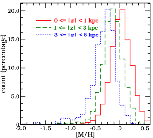
Given this large span of distances, we can investigate the change in metallicity as we move out of the Galactic plane. Since we still have stars with non-negligible errors in distance, this analysis will be subject to contamination from stars at different distances, so we show only the relevant trends in our data. The resulting distribution of metallicity for three $|z|$ bins is shown in Fig. 11 for stars with relative distance error less than 75%. It is clear that most of the stars in the $|z|<1$ kpc bin are consistent with a solar-metallicity thin-disk population, but as we move away from the plane the mean metallicity decreases. In particular, a tail of metal-poor stars is evident for $|z|>3$ kpc, consistent with a halo population. The trends that we are seeing are similar to those seen by Ivezić et al. (2008), where the metal-poor halo becomes apparent at [M/H] $\la-1$ for $|z|\ga 2$ kpc.

Figure 10: The RAVE stars in galactic coordinates, the circle with label GC indicates the galactic centre (which we have assumed to be at a distance of 8 kpc from the Sun). We have only plotted those stars with distance error less than 40%.

Figure 11: Normalised metallicity distribution for stars in different bins of height above the Galactic plane, where we are only showing stars with distance error less than 75%. As expected, stars further away from the Galactic plane are more metal poor.

We now analyse the velocities of stars in our sample, restricting ourselves to a high-quality subset of $5\,020$ stars. For this sample we only use those stars with distance error less than 40%, proper motion error less than 5 ${\rm mas}\,{\rm yr}^{-1}$ (in both components) and radial velocity error less than 5 ${\rm km\,s}^{-1}$.

In Fig. 12 we have plotted the average $v_{\phi}$ (where $-220$ ${\rm km\,s}^{-1}$ corresponds to the LSR) in different bins of $|z|$. It shows a decreasing rotational velocity as we move away from the Galactic plane, which can be explained by a transition from a fast rotating disk component, to a non-rotating (or slowly-rotating) halo. As before, owing to our uncertainties in the giant distances, this plot should only be used to draw qualitative conclusions.

Figure 12: Rotational velocity as a function of $|z|$ for the high-quality subset of 5 020 stars (see §4). The error bars indicate $1\sigma$ uncertainty in the means. Note that the LSR has been assumed to move with $v_{\phi}=-220$ ${\rm km\,s}^{-1}$.

Figure 13: Velocity distributions for the $U$, $V$ and $W$ components (histogram) and the best fit Gaussian (solid line) for high-quality volume-limited sample of 3 249 stars (see §4). The velocity distributions for $U$ and $W$ are symmetric, showing a slight negative mean $U$ and $W$ owing to the solar motion with respect to the LSR. As expected, the $V$ component shows an slight asymmetry, having a longer tail towards the slower rotating stars.

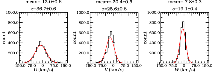
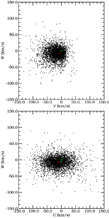
For nearby dwarfs ($\log(g){}>4$) the errors in velocity are relatively small, therefore we refine our sample further by considering a volume-limited sample. We use a cylindrical volume centred on the Sun with a radius of 500 pc and a height of 600 pc (300 above and below the Galactic plane). This sample, which contains 3 249 stars, has average errors of $(8.2\leavevmode\nobreak\ \text{${\rm km\,s}^{-1}$},\,6.3\leavevmode\nobreak\ \text{${\rm km\,s}^{-1}$},\,5.1\leavevmode\nobreak\ \text{${\rm km\,s}^{-1}$})$ in the $(U,\,V,\,W)$ directions, respectively. The velocity distributions for these stars are shown in Fig. 13 and the corresponding means and velocity dispersions are given in Table 1. The uncertainties are obtained by a bootstrap method. Note that these distributions will be broadened by the observational errors, but we have not taken this into account when calculating these variances. For this sample, we also tabulate the full velocity dispersion tensor $\sigma_{ij}$. As has been found by previous studies (e.g. Dehnen & Binney 1998), the $\sigma_{UV}$ term is clearly non-zero ($\sigma^{2}_{UV}=108.0\pm 25.7\leavevmode\nobreak\ \textrm{km${}^{2}$\,s${}^{-2}$}$). For this component we can calculate the vertex deviation,

$$l_{v}=\frac{1}{2}\arctan\left(2\frac{\sigma_{UV}^{2}}{\sigma_{U}^{2}-\sigma_{V}^{2}}\right),$$ (6)

which is a measure of the orientation of the $UV$ velocity ellipsoid. We find $l_{v}=8.7\pm 2.0^{\circ}$, which is comparable to the value of $10^{\circ}$ found for stars with $(B-V)\ga 0.4$ in the immediate solar neighbourhood by Dehnen & Binney (1998). The uncertainties on the other two cross-terms ($\sigma_{UW}^{2}$ and $\sigma_{VW}^{2}$) are too large to allow us to detect any weak correlations that might be present.

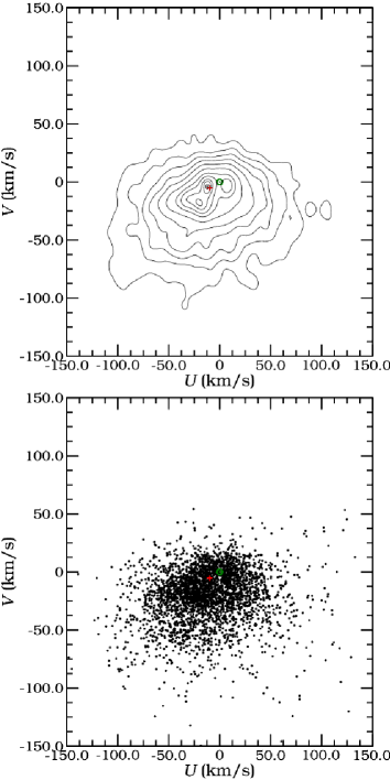
Close inspection of the middle panel of Fig. 13 shows an asymmetric distribution for the $V$ component, with a longer tail towards lower velocities. This is due to two effects. The first is that we are seeing the well-known asymmetric drift, where populations of stars with larger velocity dispersions lag behind the LSR (Binney & Merrifield 1998). Secondly, it is known that the velocity distribution of the solar neighbourhood is not smooth (see, e.g. Chereul et al. 1998; Dehnen 1998; Nordström et al. 2004). This issue is further illustrated in Fig. 14, where we show the distribution of velocities in the $UV$-plane. A slight over-density of stars around $U\approx-50$ ${\rm km\,s}^{-1}$, $V\approx-50$ ${\rm km\,s}^{-1}$ can be seen which will affect the symmetry of the $V$ velocity component. This over-density is called the Hercules stream, and is thought to be due to a resonance with the bar of our Galaxy (Dehnen 2000; Fux 2001).

It should be noted that all velocities are with respect to the Sun, which implies that the Sun’s $U$ and $W$ velocity with respect to the LSR are the negative of the mean $U$ and $W$ in our sample. Due to the asymmetric drift, the $V$ velocity of the complete sample of stars is not equal to the negative of the $V$ velocity of Sun with respect to the LSR (Binney & Merrifield 1998). The velocities and dispersions are in reasonable agreement with the results of Famaey et al. (2005) and Dehnen & Binney (1998) even though we are using different samples from those examined in these previous studies (e.g. probing different volumes or types of stars).

Mean	$\overline{U}$	$\overline{V}$	$\overline{W}$
(${\rm km\,s}^{-1}$)	$-12.0\pm 0.6$	$-20.4\pm 0.5$	$-7.8\pm 0.3$
Standard Deviation	$\sigma_{U}$	$\sigma_{V}$	$\sigma_{W}$
(${\rm km\,s}^{-1}$)	$36.7\pm 0.6$	$25.6\pm 0.8$	$19.1\pm 0.4$
Covariance	$\sigma^{2}_{UV}$	$\sigma^{2}_{UW}$	$\sigma^{2}_{VW}$
$(\textrm{km${}^{2}$\,s${}^{-2}$})$	$108.0\pm 25.7$	$-19.7\pm 17.3$	$12.8\pm 16.2$

Table 1: Means, standard deviations and covariances for $U$, $V$ and $W$ velocities corresponding to the high-quality volume limited sample of 3 249 stars (see §4).

Figure 14: The $UV$, $UW$ and $VW$ velocity distributions for the high-quality volume-limited sample of 3 249 stars (see §4). The upper-left panel shows isodensity contours for the $UV$ plane, where the contours contain 2, 6, 12, 21, 33, 50, 68, 80, 90, 99 and 99.9 percent of the stars. The red $+$ symbol marks the LSR (Dehnen & Binney 1998) and the green $\odot$ symbol marks the solar velocity $(0,0)$.

5 Discussion

5.1 The influence of the choice of stellar models

Figure 15: A comparison of isochrones from three separate groups: Yale-Yonsei (black), Padova (red), Dartmouth (green). We have chosen isochrones with age 5 Gyr, Z = 0.019, ${[\alpha\text{/Fe}]}$ = 0.

The method described in §2.2 clearly relies on the ability of stellar models to accurately predict the observed parameters. Therefore it is worth briefly discussing the potential difficulties which may arise from this assumption.

As was discussed in §2.2 we have chosen to use the Yale-Yonsei ($Y^{2}$) models (Demarque et al. 2004), but there are several groups who make stellar models. In Fig. 15 we compare isochrones (with age 5 Gyr, $Z=0.019$, ${[\alpha\text{/Fe}]}=0$) from the following three groups: the $Y^{2}$ group (Demarque et al. 2004), the Padova group (Marigo et al. 2008) and the Dartmouth group (Dotter et al. 2008). The latter paper can be consulted for a more detailed comparison of the various groups’ theoretical models (see also Glatt et al. 2008).

In general the three curves in the $\log(T_{\text{eff}})$-$\log(g)$ plane and $\log(T_{\text{eff}})$-$M_{J}$ plane show reasonably good agreement, certainly within the observational errors of the RAVE data (see §3.1). The largest discrepancy is for the cool dwarfs ($\log(T_{\text{eff}})<3.65$), but we do not believe this should have any significant effect on our results as we have very few stars in this regime. When one considers the ${(J-K_{s})}$-$M_{J}$ plane the situation is less satisfactory, probably due to the $T_{\text{eff}}$-colour transformations.

To assess whether our decision to use the $Y^{2}$ models has any serious effect on our results, we repeat the analysis presented in Section 3.3 using the Dartmouth models. We find that this has very little influence; there is no noticeable improvement for either the Hipparcos dwarfs or the M67 giants. Therefore we conclude that our method is not particularly sensitive to the choice of stellar models. However, one should still bear in mind that, by definition, our method will be limited by any problems or deficiencies in the adopted set of isochrones.

5.2 Comparisons to other work

Figure 16: Cumulative distribution of $\log(g)$, the black line shows the % of stars below a certain $\log(g)$, while the dashed grey line shows stars above a certain $\log(g)$.

Klement et al. (2008, hereafter K08) have used a different method to derive distances for RAVE stars, seemingly obtaining significantly smaller errors than ours. They calibrated a photometric distance relation (relating $V_{T}-H$ to $M_{V}$) using stars from Hipparcos catalogue with accurate trigonometric parallaxes, combined with photometry from Tycho-2, USNO-B and 2MASS. This method was then applied to the first RAVE data release (DR1; Steinmetz et al. 2006). Although the number of stars analysed by K08 is similar to that considered here ($\sim 25\,000$), they obtain $\sim 7\,000$ stars with distance errors smaller than 25%, while we have only 431 stars with distance errors smaller than 25%.

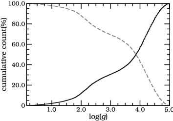
The K08 method relies on stars being on the main sequence. However, from the values of $\log(g)$we can now show that of order half the RAVE stars are giants: in Fig. 16 we show the cumulative distribution of $\log(g)$, showing that main-sequence stars ($\log(g)>4$, see also Fig. 1) are only $\sim 40$% of the whole sample. Therefore it is clear that a large fraction of the RAVE sample are giants, subgiants or close to the main-sequence turn-off. This will undoubtedly affect the results presented in K08. For example, their plot of the $UW$ velocity distribution is evidently suffering from significant systematics as can be seen from the correlation between the $U$ and $W$ velocities. Previous studies of local samples of stars have not found such a correlation. Our distribution of $UW$ shows no such strong correlation (Fig. 14) and $\sigma_{UW}$ is consistent with 0. Even in samples of stars out of the plane where one might expect correlations to appear, there is no evidence for such a pronounced level of correlation (Siebert et al. 2008).

As well as the problem of misclassified giant stars, additional factors that will adversely affect the K08 distances include: the metallicity distribution of the local RAVE sample will probably differ from that of Hipparcos due to the fact that RAVE probes a different magnitude range (and hence volume); or that K08 use the $V$-band which is more prone to reddening than our choice of ${(J-K_{s})}$. With regard to this latter point, we can repeat the simple analysis presented in Section 2.2. For a typical star 250 pc away, given the RAVE field-of-view the dust maps of Schlegel et al. (1998) predict extinction of $\sim 0.1$ mag in $V$ (with corresponding distance error of $\sim 5\%$) and reddening of $\sim 0.1$ mag in $(V-H)$.

6 Conclusion

We have presented a method to derive absolute magnitudes, and therefore distances, for RAVE stars using stellar models. It is based on the use of stellar model fitting in metallicity, $\log(g)$, $T_{\text{eff}}$ and colour space.

We find that our method reliably estimates distances for main-sequence stars, but there is an indication of potential systematic problems with giant stars owing to issues with the underlying stellar models. The uncertainties in the estimated absolute magnitudes for RGB stars are found to depend mainly on the uncertainties in $\log(g)$, while for main-sequence stars the accuracy of $T_{\text{eff}}$ is also important (§2.3). For the RAVE data the uncertainties in $\log(g)$ and $T_{\text{eff}}$ give rise to relative distance uncertainties in the range 30%-50%, although from cross-matching with Hipparcos (§3.3.1) it appears that our uncertainties may be overestimated for the brighter stars (with higher signal-to-noise spectra). It is important to note that that some 10% of the RAVE stars may be on the red clump, but these are treated as RGB by our pipeline, and hence their distances may be systematically biased.

As can be seen in the results section (§4), the data accurately reflect the known properties of halo and disk stars of the Milky Way. A variation in metallicity and $v_{\phi}$ was found away from the Galactic plane, corresponding to an increase in the fraction of metal-poor halo stars. Existing substructure in the $UV$ velocity plane was recovered, as was the vertex deviation. Upon completion the RAVE survey will have observed a factor of up to $\sim$20 times more stars than analysed here. Clearly this will be a hugely valuable resource for studies of the Galaxy.

In future the Gaia satellite mission (Perryman et al. 2001) will revolutionise this field, recording distances to millions of stars with unprecedented accuracy. However, for large numbers of Gaia stars it will not be possible to accurately constrain the distance due to them being too far away or too faint, which implies that it is crucial to develop techniques such as ours for reliably estimating distances.

In the near term it will be possible to improve the accuracy of our pipeline by calibrating it through observations of clusters; a technique which has been used with great success by the Sloan Digital Sky Survey (Ivezić et al. 2008). Within the RAVE collaboration a project is underway to obtain data for cluster stars (e.g. Kiss et al. 2007) and we aim to incorporate this into future analyses. This may allow us to reduce or remove the reliance on stellar models, which will lessen one of the major sources of uncertainty in our work. Our pipeline will allow us to fully utilise current surveys such as RAVE, and also places us in an ideal position exploit future large-scale spectroscopic surveys that will be enabled by upcoming instruments such as LAMOST.

Appendix A Description of RAVE catalogue with phase-space coordinates

We present the results of our distance determinations and corresponding phase-space coordinates as a comma separated values (CSV) file, with headers. The columns are described in Table 2. See Steinmetz et al. (2006); Zwitter et al. (2008) for a more detailed description of the RAVE data.

Table 2: A full description of the catalogue.

Field name	Units	Type	Description
OBJECT_ID		string	RAVE internal identifier
RA	deg	float	Right ascension (J2000)
DE	deg	float	Declination (J2000)
Glon	deg	float	Galactic longitude
Glat	deg	float	Galactic latitude
RV	${\rm km\,s}^{-1}$	float	Weighted mean of available radial velocities
eRV	${\rm km\,s}^{-1}$	float	Weighted error of available radial velocities
pmRA	mas yr-1	float	Proper motion RA
pmDE	mas yr-1	float	Proper motion DE
epmRA	mas yr-1	float	Error proper motion RA
epmDE	mas yr-1	float	Error proper motion DE
Teff	Kelvin	float	Arithmetic mean of available temperatures
nTeff		int	Number of observations having $T_{\text{eff}}$
logg	$\log(\frac{cm}{s^{2}})$	float	Arithmetic mean of available surface gravities
nlogg		int	Number of observations having $\log(g)$
MH	dex	float	Arithmetic mean of RAVE uncalibrated metallicity ([m/H])
			abundance
nMH		int	Number of observations having [m/H]
MHcalib	dex	float	Arithmetic mean of RAVE calibrated metallicity ([M/H])
			abundance
nMHcalib		int	Number of observations having [M/H]
AM	dex	float	Arithmetic mean of RAVE alpha enhancement (${[\alpha\text{/Fe}]}$)
nAM		int	Number of observations having ${[\alpha\text{/Fe}]}$
Jmag	mag	float	2MASS $J$ magnitude
eJmag	mag	float	error on Jmag
Kmag	mag	float	2MASS $K_{s}$ magnitude
eKmag	mag	float	error on Kmag
Mj	mag	float	Absolute magnitude in $J$ band (from fitting method)
eMj	mag	float	Error on $M_{J}$
distance	kpc	float	Distance from $M_{J}$ and $J$
edistance	kpc	float	Error on distance
xGal	kpc	float	Galactic $x$ coordinate
exGal	kpc	float	Error on $x$
yGal	kpc	float	Galactic $y$ coordinate
eyGal	kpc	float	Error on $y$
zGal	kpc	float	Galactic $z$ coordinate
ezGal	kpc	float	Error on $z$
U	${\rm km\,s}^{-1}$	float	Galactic velocity on $x^{\prime}$ direction w.r.t the Sun ($U$)
eU	${\rm km\,s}^{-1}$	float	Error on $U$
V	${\rm km\,s}^{-1}$	float	Galactic velocity on $y^{\prime}$ direction w.r.t the Sun ($V$)
eV	${\rm km\,s}^{-1}$	float	Error on $V$
W	${\rm km\,s}^{-1}$	float	Galactic velocity on $z^{\prime}$ direction w.r.t the Sun ($W$)
eW	${\rm km\,s}^{-1}$	float	Error on $W$
vxGal	${\rm km\,s}^{-1}$	float	Galactic velocity on $x$ direction in Galactic rest frame ($v_{x}$)
evxGal	${\rm km\,s}^{-1}$	float	Error on $v_{x}$
vyGal	${\rm km\,s}^{-1}$	float	Galactic velocity on $y$ direction in Galactic rest frame ($v_{y}$)
evyGal	${\rm km\,s}^{-1}$	float	Error on $v_{y}$
vzGal	${\rm km\,s}^{-1}$	float	Galactic velocity on $z$ direction in Galactic rest frame ($v_{z}$)
evzGal	${\rm km\,s}^{-1}$	float	Error on $v_{z}$
Vr	${\rm km\,s}^{-1}$	float	Galactic velocity on $\rho$ direction in Galactic rest frame ($v_{\rho}$)
eVr	${\rm km\,s}^{-1}$	float	Error on $v_{\rho}$
Vphi	${\rm km\,s}^{-1}$	float	Galactic velocity on $\phi$ direction in Galactic rest frame ($v_{\phi}$)
eVphi	${\rm km\,s}^{-1}$	float	Error on $v_{\phi}$

Appendix B Coordinate systems

Figure 17: Overview of the Galactic coordinates. The Sun is found at $(x,y,z)=(-8,0,0)$. $l$ and $b$ are the Galactic sky coordinates.

Figure 18: Overview of Galactic coordinate systems. $U,V,W$ velocities are with respect to the Sun and are aligned with the $x^{\prime},y^{\prime},z^{\prime}$ coordinate system. $v_{x},v_{y},v_{z}$ are Cartesian velocities, and $v_{\rho},v_{\phi}$ are cylindrical velocities, both with respect to the Galactic rest frame.

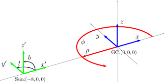
The $x^{\prime},y^{\prime},z^{\prime}$ coordinate system we use is a right handed Cartesian coordinate system centred on the Sun indicating positions, with the $x^{\prime}$ axis pointing from the Sun to the Galactic Centre (GC), the $y^{\prime}$ axis pointing in the direction of rotation and the $z^{\prime}$ axis pointing towards the Northern Galactic Pole (NGP). The $x,y,z$ coordinate system is similar to the $x^{\prime},y^{\prime},z^{\prime}$ coordinate system, but centred on the GC, assuming the Sun is at $(x,\,y,\,z)=(-8\leavevmode\nobreak\ \text{kpc},\,0,\,0)$. An overview can be found in Fig. 17 with Galactic longitude $(l)$ and latitude $(b)$ shown for completeness.

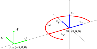
The velocities with respect to the Sun in the directions of $x,\,y,\,z$ are $U,\,V,\,W$ respectively. For velocities of nearby stars, a Cartesian coordinate system will be sufficient, but for large distances, a cylindrical coordinate system makes more sense for disk stars. To calculate these coordinates, we first have to transform the $U,\,V,\,W$ velocities to the Galactic rest frame, indicated by $v_{x},\,v_{y},\,v_{z}$ as shown in Fig. 18. Assuming a local standard of rest (LSR) of $v_{\text{LSR}}$ = 220 ${\rm km\,s}^{-1}$, and the velocity of the Sun with respect to the LSR from Dehnen & Binney (1998), we find:

$$v_{x} =U+10.0\ \mathrm{{\rm km\,s}^{-1}},$$ (7)

$$v_{y} =V+v_{\text{LSR}}+5.25\leavevmode\nobreak\ \mathrm{{\rm km\,s}^{-1}},$$ (8)

$$v_{z} =W+7.17\ \mathrm{{\rm km\,s}^{-1}}.$$ (9)

The relations between Cartesian ($x,\,y,\,z$) and cylindrical coordinates ($\rho,\,\phi,\,z)$ are:

$$x =\rho\cos(\phi),$$ (10)

$$y =\rho\sin(\phi),$$ (11)

$$z =z,$$ (12)

$$\rho^{2} =x^{2}+y^{2},$$ (13)

$$\tan(\phi) =\frac{y}{x}.$$ (14)

We can use this to find the velocities in the directions of $\rho$ and $\phi$:

$$v_{\rho} =\frac{d\rho}{dt}=\frac{xv_{x}+yv_{y}}{\rho},$$ (15)

$$v_{\phi} =\rho\frac{d\phi}{dt}=\frac{xv_{y}-yv_{x}}{\rho}.$$ (16)

Note that the direction of $\phi$ is anti-clockwise, meaning that the LSR is at $(v_{\rho},\,v_{\phi},\,v_{z})=(0\leavevmode\nobreak\ \text{${\rm km\,s}^{-1}$},\,-220\leavevmode\nobreak\ \text{${\rm km\,s}^{-1}$},\,0\leavevmode\nobreak\ \text{${\rm km\,s}^{-1}$})$.