A finite element method for second order nonvariational elliptic problems

Abstract.

We propose a numerical method to approximate the solution of second order elliptic problems in nonvariational form. The method is of Galerkin type using conforming finite elements and applied directly to the nonvariational (nondivergence) form of a second order linear elliptic problem. The key tools are an appropriate concept of “finite element Hessian” and a Schur complement approach to solving the resulting linear algebra problem. The method is illustrated with computational experiments on three linear and one quasilinear PDE, all in nonvariational form.

1. Introduction

Finite element methods (FEM) arguably constitute one of the most successful method families in numerically approximating elliptic partial differential equations (PDE’s) that are given in variational (also known as divergence) form.

For the reader’s appreciation of this statement we briefly introduce standard FEM concepts. Let $\varOmega$ be a given domain (open and bounded set) in $\mathbb{R}^{d}$, $d\in\mathbb{N}$, $f,a_{\alpha,\beta}=a_{\beta,\alpha}:\varOmega\to\mathbb{R}$, be given functions with the appropriate regularity such that the operator $\operatorname{div}\left(\boldsymbol{A}\nabla u\right)$, for $\boldsymbol{A}:=[a_{\alpha,\beta}]_{\alpha,\beta=1,\ldots,d}$, makes sense, is elliptic and there is a unique function $u:\varOmega\to\mathbb{R}$ satisfying $\operatorname{div}\left(\boldsymbol{A}\nabla u\right)=f$ with $u=0$ on $\partial\varOmega$ [GT83, for details]. The classical solution, $u$, of this problem can be characterized by first writing the PDE in weak (also known as variational) form using Green’s formula:

$$u\in\mathscr{Y}\text{ and satisfies }a(u,v):=\int_{\varOmega}{{\nabla u}^{{\boldsymbol{\intercal}}}\boldsymbol{A}\nabla v}=\int_{\varOmega}fv\quad\>\forall\>v\in\mathscr{X},$$ (1.1)

where $\mathscr{X}\text{ and }\mathscr{Y}$ are appropriate (infinite dimensional) function spaces. A (finite) Galerkin procedure consists in finding an approximation of $u$, $U\in\mathbb{Y}$

$$A(U,V)=\left\langle f,V\right\rangle\quad\>\forall\>V\in\mathbb{X},$$ (1.2)

where $\mathbb{Y}$ and $\mathbb{X}$ are finite dimensional “counterparts” (usually subspaces, but may be not) of $\mathscr{Y}$ and $\mathscr{X}$ and the bilinear form $A$ an approximation of $a$. For example, when $a=A$ (modulo quadrature) $\mathscr{X}=\mathscr{Y}=\operatorname{H}^{1}_{0}(\varOmega)$ and $\mathbb{X}=\mathbb{Y}$ are a space of continuous piecewise $p$-degree polynomial functions on a partition of $\varOmega$, we obtain the standard conforming mesh-refinement ($h$-version) finite element method of degree $p$.

The reason behind the FEM’s success in such a framework is twofold: (1) the weak form is suitable to apply functional analytic frameworks (Lax–Milgram Theorem or Babuška–Brezzi–Ladyženskaya condition, e.g.), and (2) the discrete functions need to be differentiated at most once, whence weak smoothness requirements on the “elements”.

In this article, we depart from this basis by considering second order elliptic boundary value problems (BVP’s) in nonvariational form

$$\text{find }u\text{ such that }{\boldsymbol{A}}{:}{\mathrm{D}^{2}u}=f\text{ in }\varOmega\text{ and }\left.u\right|_{\partial\varOmega}=g,$$ (1.3)

for which one may not always be successful in applying the standard FEM (with reference to §2 for the notation). Indeed, the use of the standard FEM requires (1) the coefficient matrix $\boldsymbol{A}:\varOmega\to\mathbb{R}^{d\times d}$ to be (weakly) differentiable and (2) the rewriting of the second order term in divergence form, an operation which introduces an advection (first order) term:

$${\boldsymbol{A}}{:}{\mathrm{D}^{2}u}=\operatorname{div}\left(\boldsymbol{A}\nabla u\right)-\left({\operatorname{div}\left(\boldsymbol{A}\right)}\right)\nabla u.$$ (1.4)

Even when coefficient matrix $\boldsymbol{A}$ is differentiable on $\varOmega$, this procedure could result in the problem becoming advection–dominated and unstable for conforming FEM, as we demonstrate numerically using Problem (4.5).

Our main motivation for studying linear elliptic BVP’s in nonvariational form is their important role in pure and applied mathematics. An important example of nonvariational problems is the fully nonlinear BVP that is approximated via a Newton method which becomes an infinite sequence of linear nonvariational elliptic problems [Böh08].

In this article, we propose and test a direct discretization of the strong form (1.3) that makes no special assumption on the derivative of $\boldsymbol{A}$. The main idea, is an appropriate definition of a finite element Hessian given in §2.5. The finite element Hessian has been used earlier in different contexts, such as anisotropic mesh generation [AV02, CSX07, VMD⁺07] and finite element convexity [AM08]. The finite element Hessian is related also to the finite element (discrete) elliptic operator appearing in the analysis of evolution problems [Tho06].

The method we propose is quite straightforward, and we are surprised that it is not easily available in the literature. It consists in discretizing, via a Galerkin procedure, the BVP (1.3) directly without writing it in divergence form.

The main difficulty of our approach is having to deal with a somewhat involved linear algebra problem that needs to be solved as efficiently as possible (this is especially important when we apply this method in the linearization of nonlinear elliptic BVP’s). We overcame this difficulty in §3, by combining the definition of $u$’s distributional Hessian,

$$\left\langle\mathrm{D}^{2}u\,|\,\phi\right\rangle=-\left\langle\nabla u\otimes\nabla\phi\right\rangle+\left\langle\nabla u\otimes\boldsymbol{n}\ \phi\right\rangle_{\partial{\varOmega}}\quad\>\forall\>\phi\in\operatorname{C}^{\infty}(\varOmega),$$ (1.5)

with equation (1.3) into a system of equations that are larger, but easier to handle numerically, once discretized.

It is worth noting that there are alternatives to our approach, most notably the standard finite difference method and its variants. The reason we are interested in a Galerkin procedure is the ability to use an unstructured mesh, essential for complicated geometries where the finite difference method leads to complicated, and sometimes prohibitive, modifications (especially in dimension $3$ and higher), and the potential of dealing with adaptive methods, using available finite element code. Furthermore, our method has the potential to approach the iterative solution fully nonlinear problems where finite difference methods can become clumsy and demanding [KT92, LR05, Obe08, CS08].

This paper focuses mainly on the algorithmic and linear algebraic aspects of the method and is set out as follows. In §2 we introduce some notation and set out the model problem. We then present a discretization scheme for the model problem using standard conforming finite elements in $\operatorname{C}^{0}(\varOmega)$. In §3 we present a linear algebra technique, inspired by the standard Schur complement idea, for solving the linear system arising from the discretization. Finally, in §4 we summarize extensive numerical experiments on model linear boundary value problems (BVPs) in nonvariational form and an application to quasilinear BVP in nonvariational form.

2. Set up

2.1. Notation

Let $\varOmega\subset\mathbb{R}^{d}$ be an open and bounded Lipschitz domain. We denote $\operatorname{L}_{2}(\varOmega)$ to be the space of square (Lebesgue) integrable functions on $\varOmega$ together with it’s inner product $\left\langle v,w\right\rangle:=\int_{\varOmega}vw$ and norm $\left\|v\right\|:=\left\|v\right\|_{\operatorname{L}_{2}(\varOmega)}=\left\langle v,v\right\rangle^{1/2}$. We also denote by $\langle f\rangle_{\omega}$ the integral of a function $f$ over the domain $\omega$ and drop the subscript for $\omega=\varOmega$.

We use the convention that the derivative $\mathrm{D}u$ of a function $u:\varOmega\to\mathbb{R}$ is a row vector, while the gradient of $u$, $\nabla u$ is the derivative’s transpose, i.e., $\nabla u={\left(\mathrm{D}u\right)}^{{\boldsymbol{\intercal}}}$. We will make use of the slight abuse of notation, following a common practice, whereby the Hessian of $u$ is denoted as $\mathrm{D}^{2}u$ (instead of the correct $\nabla\mathrm{D}u$) and is represented by a $d\times d$ matrix.

The Sobolev spaces  [Cia78, Eva98]

$$\operatorname{H}^{k}(\varOmega):=\operatorname{W}^{k}_{2}(\varOmega)=\left\{\phi\in\operatorname{L}_{2}(\varOmega):\;\sum_{\left|\boldsymbol{\alpha}\right|\leq k}\mathrm{D}^{\boldsymbol{\alpha}}\phi\in\operatorname{L}_{2}(\varOmega)\right\},$$ (2.1)

are equipped with norms and semi-norms

$$\left\|v\right\|_{k}^{2}:=\left\|v\right\|_{\operatorname{H}^{k}(\varOmega)}^{2}=\sum_{\left|\boldsymbol{\alpha}\right|\leq k}\left\|\mathrm{D}^{\boldsymbol{\alpha}}v\right\|^{2}$$ (2.2)

$$\text{ and }\left|v\right|_{k}^{2}:=\left|v\right|_{\operatorname{H}^{k}(\varOmega)}^{2}=\sum_{\left|\boldsymbol{\alpha}\right|=k}\left\|\mathrm{D}^{\boldsymbol{\alpha}}v\right\|^{2}$$ (2.3)

respectively, where $\boldsymbol{\alpha}=\{\alpha_{1},...,\alpha_{d}\}$ is a multi-index, $\left|\boldsymbol{\alpha}\right|=\sum_{i=1}^{d}\alpha_{i}$ and derivatives $\mathrm{D}^{\boldsymbol{\alpha}}$ are understood in a weak sense. We pay particular attention to the cases $k=1,2$,

$$\operatorname{H}^{1}_{0}(\varOmega):=\text{closure of }\operatorname{C}^{\infty}_{0}(\varOmega)\text{ in }\operatorname{H}^{1}(\varOmega)$$ (2.4)

$$\text{ and }\operatorname{H}^{-1}(\varOmega):=\operatorname{dual}\left({\operatorname{H}^{1}_{0}(\varOmega)}\right).$$ (2.5)

We denote by $\left\langle v\,|\,w\right\rangle$ the action of a distribution $v$ on the function $w$. If both $v,w\in\operatorname{L}_{2}(\varOmega)$ then $\left\langle v\,|\,w\right\rangle=\left\langle v,w\right\rangle$.

We consider the following problem: Find $u\in\operatorname{H}^{1}_{0}(\varOmega)$ such that

$$\begin{split}\mathscr{L}u&=f\text{ in }\varOmega,\\ u&=0\text{ on }\partial\varOmega,\end{split}$$ (2.6)

where the data $f:\varOmega\to\mathbb{R}$ is prescribed and $\mathscr{L}$ is a general linear, second order, uniformly elliptic partial differential operator. Let $\boldsymbol{A}\in\operatorname{L}_{\infty}(\varOmega)^{d\times d}\cap\operatorname{Sym}(\mathbb{R}^{d\times d})$, the space of bounded, symmetric, positive definite, $d\times d$ matrixes.

$$\begin{array}[]{rccl}{\mathscr{L}}:&{\operatorname{H}^{1}_{0}(\varOmega)}&\to&{\operatorname{H}^{-1}(\varOmega)}\\ &{u}&\mapsto&{\mathscr{L}u:={\boldsymbol{A}}{:}{\mathrm{D}^{2}u},}\end{array}\quad$$ (2.7)

we use ${\boldsymbol{X}}{:}{\boldsymbol{Y}}:=\operatorname{trace}{({\boldsymbol{X}}^{{\boldsymbol{\intercal}}}\boldsymbol{Y})}$ to denote the Frobenius inner product between two matrixes.

2.2. Discretization

Let $\mathscr{T}$ be a conforming triangulation of $\varOmega$, namely, $\mathscr{T}$ is a finite family of sets such that

1. $K\in\mathscr{T}$ implies $K$ is an open simplex (segment for $d=1$, triangle for $d=2$, tetrahedron for $d=3$),

2. for any $K,J\in\mathscr{T}$ we have that $\overline{K}\cap\overline{J}$ is a full subsimplex (i.e., it is either $\emptyset$, a vertex, an edge, a face, or the whole of $\overline{K}$ and $\overline{J}$) of both $\overline{K}$ and $\overline{J}$ and

3. $\bigcup_{K\in\mathscr{T}}\overline{K}=\overline{\varOmega}$.

The shape regularity of $\mathscr{T}$ is defined as

$$\mu(\mathscr{T}):=\inf_{K\in\mathscr{T}}\frac{\rho_{K}}{h_{K}},$$ (2.8)

where $\rho_{K}$ is the radius of the largest ball contained inside $K$ and $h_{K}$ is the diameter of $K$. We use the convention where $h:\varOmega\to\mathbb{R}$ denotes the meshsize function of $\mathscr{T}$, i.e.,

$$h(\boldsymbol{x}):=\max_{\overline{K}\ni\boldsymbol{x}}h_{K}.$$ (2.9)

We introduce the finite element spaces

$$\mathbb{V}:=\left\{\Phi\in\operatorname{H}^{1}(\varOmega):\;\Phi|_{K}\in\mathbb{P}^{p}\>\forall\>K\in\mathscr{T}\right\},$$ (2.10)

$$\mathring{\mathbb{V}}:=\mathbb{V}\cap\operatorname{H}^{1}_{0}(\varOmega),$$ (2.11)

where $\mathbb{P}^{k}$ denotes the linear space of polynomials in $d$ variables of degree no higher than a positive integer $k$. We consider $p\geq 1$ to be fixed and denote by $\mathring{N}:=\dim{\mathring{\mathbb{V}}}$ and $N=\mathring{N}+{N}_{\partial{}}:=\dim{\mathbb{V}}$. Let ${\boldsymbol{\mathsf{\mathring{\Phi}}}}={(\mathring{\Phi}_{1},...,\mathring{\Phi}_{\mathring{N}})}^{{\boldsymbol{\intercal}}}$ and ${\boldsymbol{\mathsf{\Phi}}}={(\mathring{\Phi}_{1},...,\mathring{\Phi}_{\mathring{N}},\Phi_{1},...,\Phi_{{N}_{\partial{}}})}^{{\boldsymbol{\intercal}}}$ where $\{\mathring{\Phi}_{1},...,\mathring{\Phi}_{\mathring{N}}\}$ and $\{\mathring{\Phi}_{1},...,\mathring{\Phi}_{\mathring{N}},\Phi_{1},...,\Phi_{{N}_{\partial{}}}\}$ form a basis of $\mathring{\mathbb{V}}$, $\mathbb{V}$ respectively.

Testing the model problem (2.6) with $\phi\in\operatorname{H}^{1}_{0}(\varOmega)$ gives

$$\left\langle\mathscr{L}u,\phi\right\rangle=\left\langle{\boldsymbol{A}}{:}{\mathrm{D}^{2}u},\phi\right\rangle=\left\langle f,\phi\right\rangle.$$ (2.12)

In order to discretize (2.12) with $\mathbb{V}$ we use an appropriate definition of a Hessian of a finite element function. Such a function may not admit a Hessian in the classical sense, so we consider it as a distribution (or generalized function) which we recall the definition.

2.3 Definition (generalized Hessian).

Let $\boldsymbol{n}:\partial\varOmega\to\mathbb{R}^{d}$ be the outward pointing normal of $\varOmega$. Given $v\in\operatorname{H}^{1}_{0}(\varOmega)$ its generalized Hessian defined in the standard distributional sense is given by

$$\left\langle\mathrm{D}^{2}v\,|\,\phi\right\rangle=-\left\langle\nabla v\otimes\nabla\phi\right\rangle+\left\langle\nabla v\otimes\boldsymbol{n}\ \phi\right\rangle_{\partial\varOmega}\quad\>\forall\>\phi\in\operatorname{C}^{\infty}(\varOmega),$$ (2.13)

where we are using $\boldsymbol{x}\otimes\boldsymbol{y}:={\boldsymbol{x}}{{\boldsymbol{y}}^{{\boldsymbol{\intercal}}}}$ to denote the tensor product between two geometric vectors $\boldsymbol{x}\text{ and }\boldsymbol{y}$.

2.4 Theorem (finite element Hessian).

For each $V\in\mathring{\mathbb{V}}$ there exists a unique $\boldsymbol{H}[V]\in\mathbb{V}^{d\times d}$ such that

$$\left\langle\boldsymbol{H}[V],\Phi\right\rangle=\left\langle\mathrm{D}^{2}V\,|\,\Phi\right\rangle\quad\>\forall\>\Phi\in\mathbb{V}.$$ (2.14)

Proof . Given a finite element function $V\in\mathring{\mathbb{V}}$, Definition 2.3 implies

$$\left\langle\mathrm{D}^{2}V\,|\,\phi\right\rangle=-\left\langle\nabla V\otimes\nabla\phi\right\rangle+\left\langle\nabla V\otimes\boldsymbol{n}\ \phi\right\rangle_{\partial\varOmega}\quad\>\forall\>\phi\in\operatorname{C}^{\infty}(\varOmega).$$ (2.15)

We fix $V$ and let

$$\begin{array}[]{rccl}{G}:&{\operatorname{C}^{\infty}(\varOmega)}&\to&{\mathbb{R}^{d\times d}}\\ &{\phi}&\mapsto&{-\left\langle\nabla V\otimes\nabla\phi\right\rangle+\left\langle\nabla V\otimes\boldsymbol{n}\ \phi\right\rangle_{\partial\varOmega}.}\end{array}\quad$$ (2.16)

Notice that $G$ is a bounded linear functional on $\operatorname{C}^{\infty}(\varOmega)$ in the $\operatorname{H}^{1}(\varOmega)$-norm as,

$$\left|G(\phi)\right|=\left|\left\langle\nabla V\otimes\nabla\phi\right\rangle\right|+\left|\left\langle\nabla V\otimes\boldsymbol{n}\ \phi\right\rangle_{\partial\varOmega}\right|\leq C(d,\varOmega)\left\|V\right\|_{1}\left\|\phi\right\|_{1}.$$ (2.17)

Thus, due to the density of $\operatorname{C}^{\infty}(\varOmega)$ in $\operatorname{H}^{1}(\varOmega)$, $G$ admits a unique extension, $\tilde{G}$.

Let $R=\left.\tilde{G}\right|_{\mathbb{V}}$ be the restriction of $\tilde{G}$ to $\mathbb{V}$. Since $\tilde{G}$ is linear and bounded on $\operatorname{H}^{1}(\varOmega)$ it follows that $R$ is linear and bounded on $\mathbb{V}$ in the $\operatorname{H}^{1}(\varOmega)$-norm. Hence by Riesz’s Representation Theorem there exists an $\boldsymbol{H}[V]\in\mathbb{V}^{d\times d}$ such that for each $\Phi\in\mathbb{V}$

$$\left\langle\boldsymbol{H}[V],\Phi\right\rangle:=R(\Phi)=-\left\langle\nabla V\otimes\nabla\Phi\right\rangle+\left\langle\nabla V\otimes\boldsymbol{n}\ \Phi\right\rangle_{\partial\varOmega},$$ (2.18)

which coincides with the generalized Hessian (cf. Definition 2.3) on $\mathbb{V}$. ∎

2.5 Definition (finite element Hessian).

From Theorem 2.4 we define the finite element Hessian as follows. Let $V\in\mathring{\mathbb{V}}$ then

$$\left\langle\boldsymbol{H}[V],\Phi\right\rangle:=-\left\langle\nabla V\otimes\nabla\Phi\right\rangle+\left\langle\nabla V\otimes\boldsymbol{n}\ \Phi\right\rangle_{\partial\varOmega}\quad\>\forall\>\Phi\in\mathbb{V}.$$ (2.19)

It follows that $\boldsymbol{H}$ is a linear operator on $\mathring{\mathbb{V}}$.

Taking the model problem (2.12) we substitute the finite element Hessian directly, reducing the space of test functions to $\mathring{\mathbb{V}}$, we wish to find $U\in\mathring{\mathbb{V}}$ such that

$$\left\langle{\boldsymbol{A}}{:}{\boldsymbol{H}[U]},\mathring{\Phi}\right\rangle=\left\langle f,\mathring{\Phi}\right\rangle\quad\>\forall\>\mathring{\Phi}\in\mathring{\mathbb{V}}.$$ (2.20)

2.6 Theorem (nonvariational finite element method (NVFEM)).

The nonvariational finite element solution for the model problem’s discretization (2.20) is given as $U={{\boldsymbol{\mathsf{\mathring{\Phi}}}}}^{{\boldsymbol{\intercal}}}{\boldsymbol{\mathsf{u}}}$, where ${\boldsymbol{\mathsf{u}}}\in\mathbb{R}^{\mathring{N}}$ is the solution to the following linear system

$${\boldsymbol{\mathsf{D}}}{\boldsymbol{\mathsf{u}}}:=\sum_{\alpha=1}^{d}\sum_{\beta=1}^{d}{\boldsymbol{\mathsf{B}}}^{\alpha,\beta}{\boldsymbol{\mathsf{M}}}^{-1}{\boldsymbol{\mathsf{C}}}_{\alpha,\beta}{\boldsymbol{\mathsf{u}}}={\boldsymbol{\mathsf{f}}}.$$ (2.21)

The components of (2.21) are given by

$${\boldsymbol{\mathsf{B}}}^{\alpha,\beta} :=\left\langle{\boldsymbol{\mathsf{\mathring{\Phi}}}},\boldsymbol{A}^{\alpha,\beta}{{\boldsymbol{\mathsf{\Phi}}}}^{{\boldsymbol{\intercal}}}\right\rangle\in\mathbb{R}^{\mathring{N}\times N},$$ (2.22)

$${\boldsymbol{\mathsf{M}}} :=\left\langle{\boldsymbol{\mathsf{\Phi}}},{{\boldsymbol{\mathsf{\Phi}}}}^{{\boldsymbol{\intercal}}}\right\rangle\in\mathbb{R}^{N\times N},$$ (2.23)

$${\boldsymbol{\mathsf{C}}}_{\alpha,\beta} :=-\left\langle\partial_{\beta}{{\boldsymbol{\mathsf{\Phi}}}},\partial_{\alpha}{}{{\boldsymbol{\mathsf{\mathring{\Phi}}}}}^{{\boldsymbol{\intercal}}}\right\rangle+\left\langle{\boldsymbol{\mathsf{\Phi}}}n_{\beta},\partial_{\alpha}{{{\boldsymbol{\mathsf{\mathring{\Phi}}}}}^{{\boldsymbol{\intercal}}}}\right\rangle_{\partial\varOmega}\in\mathbb{R}^{N\times\mathring{N}},$$ (2.24)

$${\boldsymbol{\mathsf{f}}} :=\left\langle f,{{\boldsymbol{\mathsf{\mathring{\Phi}}}}}\right\rangle\in\mathbb{R}^{\mathring{N}}.$$ (2.25)

Proof . Since $\boldsymbol{H}[U]\in\mathbb{V}^{d\times d}$ for each $\alpha,\beta=1,\dots,d$ , $\boldsymbol{H}_{\alpha,\beta}[U]={{\boldsymbol{\mathsf{\Phi}}}}^{{\boldsymbol{\intercal}}}{\boldsymbol{\mathsf{h}}}_{\alpha,\beta}$. Then, testing (2.20) with ${\boldsymbol{\mathsf{\mathring{\Phi}}}}$,

$$\begin{split}\left\langle f,{\boldsymbol{\mathsf{\mathring{\Phi}}}}\right\rangle&=\sum_{\alpha=1}^{d}\sum_{\beta=1}^{d}\left\langle\boldsymbol{A}^{\alpha,\beta}\boldsymbol{H}_{\alpha,\beta}[U],{\boldsymbol{\mathsf{\mathring{\Phi}}}}\right\rangle\\ &=\sum_{\alpha=1}^{d}\sum_{\beta=1}^{d}\left\langle{\boldsymbol{\mathsf{\mathring{\Phi}}}},\boldsymbol{A}^{\alpha,\beta}{{\boldsymbol{\mathsf{\Phi}}}}^{{\boldsymbol{\intercal}}}{\boldsymbol{\mathsf{h}}}_{\alpha,\beta}\right\rangle\\ &=\sum_{\alpha=1}^{d}\sum_{\beta=1}^{d}\left\langle{\boldsymbol{\mathsf{\mathring{\Phi}}}},\boldsymbol{A}^{\alpha,\beta}{{\boldsymbol{\mathsf{\Phi}}}}^{{\boldsymbol{\intercal}}}\right\rangle{{\boldsymbol{\mathsf{h}}}_{\alpha,\beta}}.\\ &=\sum_{\alpha=1}^{d}\sum_{\beta=1}^{d}{\boldsymbol{\mathsf{B}}}^{\alpha,\beta}{\boldsymbol{\mathsf{h}}}_{\alpha,\beta}\end{split}$$ (2.26)

Utilizing Definition 2.5 for each $\alpha,\beta=1\dots d$ we can compute ${\boldsymbol{\mathsf{h}}}_{\alpha,\beta}\in\mathbb{R}^{N}$, noting $U={{\boldsymbol{\mathsf{\mathring{\Phi}}}}}^{{\boldsymbol{\intercal}}}{\boldsymbol{\mathsf{u}}}$,

$$\begin{split}\left\langle{\boldsymbol{\mathsf{\Phi}}},{{\boldsymbol{\mathsf{\Phi}}}}^{{\boldsymbol{\intercal}}}\right\rangle{\boldsymbol{\mathsf{h}}}_{\alpha,\beta}&=\left\langle{\boldsymbol{\mathsf{\Phi}}},\boldsymbol{H}_{\alpha,\beta}[U]\right\rangle\\ &=-\left\langle\partial_{\beta}{}{\boldsymbol{\mathsf{\Phi}}},\partial_{\alpha}{U}\right\rangle+\left\langle{\boldsymbol{\mathsf{\Phi}}}\boldsymbol{n}_{\beta},\partial_{\alpha}{U}\right\rangle_{\partial\varOmega}\\ &=\left(-\left\langle\partial_{\beta}{}{\boldsymbol{\mathsf{\Phi}}},\partial_{\alpha}{{{\boldsymbol{\mathsf{\mathring{\Phi}}}}}^{{\boldsymbol{\intercal}}}}\right\rangle+\left\langle{\boldsymbol{\mathsf{\Phi}}}\boldsymbol{n}_{\beta},\partial_{\alpha}{{{\boldsymbol{\mathsf{\mathring{\Phi}}}}}^{{\boldsymbol{\intercal}}}}\right\rangle_{\partial\varOmega}\right){\boldsymbol{\mathsf{u}}}.\end{split}$$ (2.27)

Using the definition of ${\boldsymbol{\mathsf{C}}}_{\alpha,\beta}$ (2.24) and ${\boldsymbol{\mathsf{M}}}$ (2.23) we see for each $\alpha,\beta=1\dots d$

$$\begin{split}{\boldsymbol{\mathsf{M}}}{{\boldsymbol{\mathsf{h}}}_{\alpha,\beta}}&={\boldsymbol{\mathsf{C}}}_{\alpha,\beta}{{\boldsymbol{\mathsf{u}}}}\\ {{\boldsymbol{\mathsf{h}}}_{\alpha,\beta}}&={\boldsymbol{\mathsf{M}}}^{-1}{\boldsymbol{\mathsf{C}}}_{\alpha,\beta}{{\boldsymbol{\mathsf{u}}}}.\end{split}$$ (2.28)

Substituting ${\boldsymbol{\mathsf{h}}}_{\alpha,\beta}$ from (2.28) into (2.26) we obtain the desired result. ∎

2.7 Example (for $d=2$).

For a general elliptic operator in 2-D, the formulation (2.21) takes the form

$$\left({\boldsymbol{\mathsf{B}}}^{1,1}{\boldsymbol{\mathsf{M}}}^{-1}{\boldsymbol{\mathsf{C}}}_{1,1}+{\boldsymbol{\mathsf{B}}}^{2,2}{\boldsymbol{\mathsf{M}}}^{-1}{\boldsymbol{\mathsf{C}}}_{2,2}+{\boldsymbol{\mathsf{B}}}^{1,2}{\boldsymbol{\mathsf{M}}}^{-1}{\boldsymbol{\mathsf{C}}}_{1,2}+{\boldsymbol{\mathsf{B}}}^{2,1}{\boldsymbol{\mathsf{M}}}^{-1}{\boldsymbol{\mathsf{C}}}_{2,1}\right){\boldsymbol{\mathsf{u}}}={\boldsymbol{\mathsf{f}}}$$ (2.29)

3. Solving the linear system

3.1 Remark ((2.21) is difficult to solve).

Looking at the full system setting ${\boldsymbol{\mathsf{D}}}=\sum\sum{\boldsymbol{\mathsf{B}}}^{\alpha,\beta}{\boldsymbol{\mathsf{M}}}^{-1}{\boldsymbol{\mathsf{C}}}_{\alpha,\beta}$ multiplying out each of the matrixes and proceeding to solve ${\boldsymbol{\mathsf{D}}}{\boldsymbol{\mathsf{u}}}={\boldsymbol{\mathsf{f}}}$ the resulting system would not be sparse forcing the use of direct solvers.

In this section we will present a method to solve formulation (2.21) in a general setting. This method makes use of the sparsity of the component matrixes ${\boldsymbol{\mathsf{B}}}^{\alpha,\beta},{\boldsymbol{\mathsf{C}}}^{\alpha,\beta}$ and ${\boldsymbol{\mathsf{M}}}$.

3.2 Remark.

An interesting point of note is that if the mass matrix ${\boldsymbol{\mathsf{M}}}$ were diagonalized, by mass lumping, then for each $\alpha$ and $\beta$ the matrix ${\boldsymbol{\mathsf{B}}}^{\alpha,\beta}{\boldsymbol{\mathsf{M}}}^{-1}{\boldsymbol{\mathsf{C}}}_{\alpha,\beta}$ would still be sparse (albeit less so than the individual matrixes ${\boldsymbol{\mathsf{B}}}^{\alpha,\beta}$ and ${\boldsymbol{\mathsf{C}}}_{\alpha,\beta}$). Hence the system can be easily solved using existing sparse methods. However mass lumping is only applicable to $\mathbb{P}^{1}$ finite elements. For higher order finite elements it would be desirable to exploit the sparse structure of the component matrixes that make up the system.

3.3. A generalized Schur complement

We observe the matrix ${\boldsymbol{\mathsf{D}}}$ in the system (2.21) is a sum of Schur complements ${\boldsymbol{\mathsf{B}}}^{\alpha,\beta}{\boldsymbol{\mathsf{M}}}^{-1}{\boldsymbol{\mathsf{C}}}_{\alpha,\beta}$. With that in mind we introduce the $(d^{2}+1)^{2}$ block matrix

$${\boldsymbol{\mathsf{E}}}=\left[\begin{array}[]{cccccc}{\boldsymbol{\mathsf{M}}}&{\boldsymbol{\mathsf{0}}}&\dotsb&{\boldsymbol{\mathsf{0}}}&{\boldsymbol{\mathsf{0}}}&-{\boldsymbol{\mathsf{C}}}_{1,1}\\ {\boldsymbol{\mathsf{0}}}&{\boldsymbol{\mathsf{M}}}&\dotsb&{\boldsymbol{\mathsf{0}}}&{\boldsymbol{\mathsf{0}}}&-{\boldsymbol{\mathsf{C}}}_{1,2}\\ \vdots&\vdots&\ddots&\vdots&\vdots&\vdots\\ {\boldsymbol{\mathsf{0}}}&{\boldsymbol{\mathsf{0}}}&\dotsb&{\boldsymbol{\mathsf{M}}}&{\boldsymbol{\mathsf{0}}}&-{\boldsymbol{\mathsf{C}}}_{d,d-1}\\ {\boldsymbol{\mathsf{0}}}&{\boldsymbol{\mathsf{0}}}&\dots&{\boldsymbol{\mathsf{0}}}&{\boldsymbol{\mathsf{M}}}&-{\boldsymbol{\mathsf{C}}}_{d,d}\\ {\boldsymbol{\mathsf{B}}}^{1,1}&{\boldsymbol{\mathsf{B}}}^{1,2}&\dots&{\boldsymbol{\mathsf{B}}}^{d,d-1}&{\boldsymbol{\mathsf{B}}}^{d,d}&{\boldsymbol{\mathsf{0}}}\end{array}\right].$$ (3.1)

3.4 Lemma (generalized Schur complement).

Given

$${\boldsymbol{\mathsf{v}}}={\left({\boldsymbol{\mathsf{h}}}_{1,1},{\boldsymbol{\mathsf{h}}}_{1,2},\dots,{\boldsymbol{\mathsf{h}}}_{d,d-1},{\boldsymbol{\mathsf{h}}}_{d,d},{\boldsymbol{\mathsf{u}}}\right)}^{{\boldsymbol{\intercal}}},$$ (3.2)

$${\boldsymbol{\mathsf{b}}}={\left({\boldsymbol{\mathsf{0}}},{\boldsymbol{\mathsf{0}}}\dots,{\boldsymbol{\mathsf{0}}},{\boldsymbol{\mathsf{0}}},{\boldsymbol{\mathsf{f}}}\right)}^{{\boldsymbol{\intercal}}},$$ (3.3)

solving the system

$${\boldsymbol{\mathsf{D}}}{\boldsymbol{\mathsf{u}}}=\sum_{\alpha=1}^{d}\sum_{\beta=1}^{d}{\boldsymbol{\mathsf{B}}}^{\alpha,\beta}{\boldsymbol{\mathsf{M}}}^{-1}{\boldsymbol{\mathsf{C}}}_{\alpha,\beta}{\boldsymbol{\mathsf{u}}}={\boldsymbol{\mathsf{f}}},$$ (3.4)

is equivalent to solving

$${\boldsymbol{\mathsf{E}}}{\boldsymbol{\mathsf{v}}}={\boldsymbol{\mathsf{b}}}.$$ (3.5)

for ${\boldsymbol{\mathsf{u}}}$.

Proof . The proof is just block Gaussian elimination on ${\boldsymbol{\mathsf{E}}}$. Left-multiplying the first $d^{2}$ rows by ${\boldsymbol{\mathsf{M}}}^{-1}$ yields

$$\left[\begin{array}[]{cccccc}{\boldsymbol{\mathsf{I}}}&{\boldsymbol{\mathsf{0}}}&\dotsb&{\boldsymbol{\mathsf{0}}}&{\boldsymbol{\mathsf{0}}}&-{\boldsymbol{\mathsf{M}}}^{-1}{\boldsymbol{\mathsf{C}}}_{1,1}\\ {\boldsymbol{\mathsf{0}}}&{\boldsymbol{\mathsf{I}}}&\dotsb&{\boldsymbol{\mathsf{0}}}&{\boldsymbol{\mathsf{0}}}&-{\boldsymbol{\mathsf{M}}}^{-1}{\boldsymbol{\mathsf{C}}}_{1,2}\\ \vdots&\vdots&\ddots&\vdots&\vdots&\vdots\\ {\boldsymbol{\mathsf{0}}}&{\boldsymbol{\mathsf{0}}}&\dotsb&{\boldsymbol{\mathsf{I}}}&{\boldsymbol{\mathsf{0}}}&-{\boldsymbol{\mathsf{M}}}^{-1}{\boldsymbol{\mathsf{C}}}_{d,d-1}\\ {\boldsymbol{\mathsf{0}}}&{\boldsymbol{\mathsf{0}}}&\dots&{\boldsymbol{\mathsf{0}}}&{\boldsymbol{\mathsf{I}}}&-{\boldsymbol{\mathsf{M}}}^{-1}{\boldsymbol{\mathsf{C}}}_{d,d}\\ {\boldsymbol{\mathsf{B}}}^{1,1}&{\boldsymbol{\mathsf{B}}}^{1,2}&\dots&{\boldsymbol{\mathsf{B}}}^{d,d-1}&{\boldsymbol{\mathsf{B}}}^{d,d}&{\boldsymbol{\mathsf{0}}}\end{array}\right]\left[\begin{array}[]{c}{\boldsymbol{\mathsf{h}}}_{1,1}\\ {\boldsymbol{\mathsf{h}}}_{1,2}\\ \vdots\\ {\boldsymbol{\mathsf{h}}}_{d,d-1}\\ {\boldsymbol{\mathsf{h}}}_{d,d}\\ {\boldsymbol{\mathsf{u}}}\end{array}\right]=\left[\begin{array}[]{c}{\boldsymbol{\mathsf{0}}}\\ {\boldsymbol{\mathsf{0}}}\\ \vdots\\ {\boldsymbol{\mathsf{0}}}\\ {\boldsymbol{\mathsf{0}}}\\ {\boldsymbol{\mathsf{f}}}\end{array}\right].$$ (3.6)

Multiplying the $i$-th row by the $i$-th entry of the $(d^{2}+1)$-th row for $i=1,\dots,d^{2}$

$$\left[\begin{array}[]{cccccc}{\boldsymbol{\mathsf{B}}}^{1,1}&{\boldsymbol{\mathsf{0}}}&\dotsb&{\boldsymbol{\mathsf{0}}}&{\boldsymbol{\mathsf{0}}}&-{\boldsymbol{\mathsf{B}}}^{1,1}{\boldsymbol{\mathsf{M}}}^{-1}{\boldsymbol{\mathsf{C}}}_{1,1}\\ {\boldsymbol{\mathsf{0}}}&{\boldsymbol{\mathsf{B}}}^{1,2}&\dotsb&{\boldsymbol{\mathsf{0}}}&{\boldsymbol{\mathsf{0}}}&-{\boldsymbol{\mathsf{B}}}^{1,2}{\boldsymbol{\mathsf{M}}}^{-1}{\boldsymbol{\mathsf{C}}}_{1,2}\\ \vdots&\vdots&\ddots&\vdots&\vdots&\vdots\\ {\boldsymbol{\mathsf{0}}}&{\boldsymbol{\mathsf{0}}}&\dotsb&{\boldsymbol{\mathsf{B}}}^{d,d-1}&{\boldsymbol{\mathsf{0}}}&-{\boldsymbol{\mathsf{B}}}^{d,d-1}{\boldsymbol{\mathsf{M}}}^{-1}{\boldsymbol{\mathsf{C}}}_{d,d-1}\\ {\boldsymbol{\mathsf{0}}}&{\boldsymbol{\mathsf{0}}}&\dots&{\boldsymbol{\mathsf{0}}}&{\boldsymbol{\mathsf{B}}}^{d,d}&-{\boldsymbol{\mathsf{B}}}^{d,d}{\boldsymbol{\mathsf{M}}}^{-1}{\boldsymbol{\mathsf{C}}}_{d,d}\\ {\boldsymbol{\mathsf{B}}}^{1,1}&{\boldsymbol{\mathsf{B}}}^{1,2}&\dots&{\boldsymbol{\mathsf{B}}}^{d,d-1}&{\boldsymbol{\mathsf{B}}}^{d,d}&{\boldsymbol{\mathsf{0}}}\end{array}\right]\left[\begin{array}[]{c}{\boldsymbol{\mathsf{h}}}_{1,1}\\ {\boldsymbol{\mathsf{h}}}_{1,2}\\ \vdots\\ {\boldsymbol{\mathsf{h}}}_{d,d-1}\\ {\boldsymbol{\mathsf{h}}}_{d,d}\\ {\boldsymbol{\mathsf{u}}}\end{array}\right]=\left[\begin{array}[]{c}{\boldsymbol{\mathsf{0}}}\\ {\boldsymbol{\mathsf{0}}}\\ \vdots\\ {\boldsymbol{\mathsf{0}}}\\ {\boldsymbol{\mathsf{0}}}\\ {\boldsymbol{\mathsf{f}}}\end{array}\right].$$ (3.7)

Subtracting each of the first $d^{2}$ rows from the $(d^{2}+1)$-th row reduces the system into row echelon form.

$$\left[\begin{array}[]{cccccc}{\boldsymbol{\mathsf{B}}}^{1,1}&{\boldsymbol{\mathsf{0}}}&\dotsb&{\boldsymbol{\mathsf{0}}}&{\boldsymbol{\mathsf{0}}}&-{\boldsymbol{\mathsf{B}}}^{1,1}{\boldsymbol{\mathsf{M}}}^{-1}{\boldsymbol{\mathsf{C}}}_{1,1}\\ {\boldsymbol{\mathsf{0}}}&{\boldsymbol{\mathsf{B}}}^{1,2}&\dotsb&{\boldsymbol{\mathsf{0}}}&{\boldsymbol{\mathsf{0}}}&-{\boldsymbol{\mathsf{B}}}^{1,2}{\boldsymbol{\mathsf{M}}}^{-1}{\boldsymbol{\mathsf{C}}}_{1,2}\\ \vdots&\vdots&\ddots&\vdots&\vdots&\vdots\\ {\boldsymbol{\mathsf{0}}}&{\boldsymbol{\mathsf{0}}}&\dotsb&{\boldsymbol{\mathsf{B}}}^{d,d-1}&{\boldsymbol{\mathsf{0}}}&-{\boldsymbol{\mathsf{B}}}^{d,d-1}{\boldsymbol{\mathsf{M}}}^{-1}{\boldsymbol{\mathsf{C}}}_{d,d-1}\\ {\boldsymbol{\mathsf{0}}}&{\boldsymbol{\mathsf{0}}}&\dots&{\boldsymbol{\mathsf{0}}}&{\boldsymbol{\mathsf{B}}}^{d,d}&-{\boldsymbol{\mathsf{B}}}^{d,d}{\boldsymbol{\mathsf{M}}}^{-1}{\boldsymbol{\mathsf{C}}}_{d,d}\\ {\boldsymbol{\mathsf{0}}}&{\boldsymbol{\mathsf{0}}}&\dots&{\boldsymbol{\mathsf{0}}}&{\boldsymbol{\mathsf{0}}}&{\boldsymbol{\mathsf{D}}}\end{array}\right]\left[\begin{array}[]{c}{\boldsymbol{\mathsf{h}}}_{1,1}\\ {\boldsymbol{\mathsf{h}}}_{1,2}\\ \vdots\\ {\boldsymbol{\mathsf{h}}}_{d,d-1}\\ {\boldsymbol{\mathsf{h}}}_{d,d}\\ {\boldsymbol{\mathsf{u}}}\end{array}\right]=\left[\begin{array}[]{c}{\boldsymbol{\mathsf{0}}}\\ {\boldsymbol{\mathsf{0}}}\\ \vdots\\ {\boldsymbol{\mathsf{0}}}\\ {\boldsymbol{\mathsf{0}}}\\ {\boldsymbol{\mathsf{f}}}\end{array}\right].$$ (3.8)

∎

3.5 Remark (structure of the block matrix).

In fact this method for the solution of the system ${\boldsymbol{\mathsf{D}}}{\boldsymbol{\mathsf{u}}}={\boldsymbol{\mathsf{f}}}$ is not surprising given the discretization presented in the proof of Theorem 2.6 is equivalent to the following system:

$$\text{Find $U\in\mathring{\mathbb{V}}$ such that }\begin{cases}\left\langle\boldsymbol{H}[U],\Phi\right\rangle=-\left\langle\nabla U\otimes\nabla\Phi\right\rangle+\left\langle\nabla U\otimes\boldsymbol{n}\ \Phi\right\rangle_{\partial{\varOmega}}\quad\>\forall\>\Phi\in\mathbb{V}\\ \\ \left\langle{\boldsymbol{A}}{:}{\boldsymbol{H}[U]},\mathring{\Phi}\right\rangle=\left\langle f,\mathring{\Phi}\right\rangle\quad\>\forall\>\mathring{\Phi}\in\mathring{\mathbb{V}}.\end{cases}$$ (3.9)

3.6 Remark (enforcing non-trivial Dirichlet boundary values).

Given additional problem data $g\in\operatorname{H}^{1/2}(\varOmega)$, to solve

$$\begin{split}\mathscr{L}u=&f\text{ in }\varOmega,\\ u=&g\text{ on }\partial\varOmega,\end{split}$$ (3.10)

it is not immediate how to enforce the boundary conditions. If we were solving the full system ${\boldsymbol{\mathsf{D}}}{\boldsymbol{\mathsf{u}}}={\boldsymbol{\mathsf{f}}}$, we could directly enforce them into the system matrix.

Since $g\in\operatorname{H}^{1/2}(\varOmega)$ by an embedding it is continuous and can be approximated by the Lagrange interpolant with optimal order. To enforce the Dirichlet boundaries we introduce a further block representation

$$\left[\begin{array}[]{c c}{\boldsymbol{\mathsf{I}}}&{\boldsymbol{\mathsf{0}}}\\ {\boldsymbol{\mathsf{E}}}_{\partial{}}&{\boldsymbol{\mathsf{E}}}\end{array}\right]\left[\begin{array}[]{c}{\boldsymbol{\mathsf{v}}}_{\partial{}}\\ {\boldsymbol{\mathsf{v}}}\end{array}\right]=\left[\begin{array}[]{c}{\boldsymbol{\mathsf{b}}}_{\partial{}}\\ {\boldsymbol{\mathsf{b}}}\end{array}\right],$$ (3.11)

where ${\boldsymbol{\mathsf{E}}},{\boldsymbol{\mathsf{v}}}\text{ and }{\boldsymbol{\mathsf{b}}}$ are defined as before and ${\boldsymbol{\mathsf{E}}}_{\partial{}},{\boldsymbol{\mathsf{v}}}_{\partial{}}\text{ and }{\boldsymbol{\mathsf{b}}}_{\partial{}}$ are defined as follows

$${\boldsymbol{\mathsf{E}}}_{\partial{}}=\left[\begin{array}[]{c c c c c c}{\boldsymbol{\mathsf{M}}}&{\boldsymbol{\mathsf{0}}}&\dotsb&{\boldsymbol{\mathsf{0}}}&{\boldsymbol{\mathsf{0}}}&-{\boldsymbol{\mathsf{C}}}_{1,1}^{\partial{}}\\ {\boldsymbol{\mathsf{0}}}&{\boldsymbol{\mathsf{M}}}&\dotsb&{\boldsymbol{\mathsf{0}}}&{\boldsymbol{\mathsf{0}}}&-{\boldsymbol{\mathsf{C}}}_{1,2}^{\partial{}}\\ \vdots&\vdots&\ddots&\vdots&\vdots&\vdots\\ {\boldsymbol{\mathsf{0}}}&{\boldsymbol{\mathsf{0}}}&\dotsb&{\boldsymbol{\mathsf{M}}}&{\boldsymbol{\mathsf{0}}}&-{\boldsymbol{\mathsf{C}}}_{d,d-1}^{\partial{}}\\ {\boldsymbol{\mathsf{0}}}&{\boldsymbol{\mathsf{0}}}&\dots&{\boldsymbol{\mathsf{0}}}&{\boldsymbol{\mathsf{M}}}&-{\boldsymbol{\mathsf{C}}}_{d,d}^{\partial{}}\\ {\boldsymbol{\mathsf{B}}}^{1,1}&{\boldsymbol{\mathsf{B}}}^{1,2}&\dots&{\boldsymbol{\mathsf{B}}}^{d,d-1}&{\boldsymbol{\mathsf{B}}}^{d,d}&{\boldsymbol{\mathsf{0}}}\end{array}\right],$$ (3.18)

$${\boldsymbol{\mathsf{v}}}_{\partial{}}={\left[{\boldsymbol{\mathsf{h}}}_{1,1}^{\partial{}},{\boldsymbol{\mathsf{h}}}_{1,2}^{\partial{}},\dots,{\boldsymbol{\mathsf{h}}}_{d,d-1}^{\partial{}},{\boldsymbol{\mathsf{h}}}_{d,d}^{\partial{}},{\boldsymbol{\mathsf{u}}}^{\partial{}}\right]}^{{\boldsymbol{\intercal}}},$$ (3.19)

$${\boldsymbol{\mathsf{b}}}_{\partial{}}={\left[{\boldsymbol{\mathsf{0}}},{\boldsymbol{\mathsf{0}}},\dots,{\boldsymbol{\mathsf{0}}},{\boldsymbol{\mathsf{0}}},{\boldsymbol{\mathsf{g}}}\right]}^{{\boldsymbol{\intercal}}}.$$ (3.20)

Let ${\boldsymbol{\mathsf{\Phi}}}_{\partial{}}=\{\Phi_{1},\dots,\Phi_{{N}_{\partial{}}}\}$, then the components of ${\boldsymbol{\mathsf{E}}}_{\partial{}}$ and ${\boldsymbol{\mathsf{b}}}_{\partial{}}$ are defined as follows

$${\boldsymbol{\mathsf{C}}}^{\partial{}}_{\alpha,\beta}=-\left\langle\partial_{\beta}{}{\boldsymbol{\mathsf{\Phi}}},\partial_{\alpha}{}{{\boldsymbol{\mathsf{\Phi}}}_{\partial{}}}^{{\boldsymbol{\intercal}}}\right\rangle+\left\langle{\boldsymbol{\mathsf{\Phi}}}\boldsymbol{n}_{\beta},\partial_{\alpha}{}{{\boldsymbol{\mathsf{\Phi}}}_{\partial{}}}^{{\boldsymbol{\intercal}}}\right\rangle_{\partial{\varOmega}}\in\mathbb{R}^{N\times{N}_{\partial{}}},$$ (3.21)

$${\boldsymbol{\mathsf{g}}}_{j}=g(x_{j})\Phi_{j}\in\mathbb{R}^{{N}_{\partial{}}},$$ (3.22)

where $x_{j}$ is the Lagrange node associated with $\Phi_{j}$.

The block matrix (3.11) can then be trivially solved

$${\boldsymbol{\mathsf{E}}}{\boldsymbol{\mathsf{v}}}={\boldsymbol{\mathsf{b}}}-{\boldsymbol{\mathsf{E}}}_{\partial{}}{\boldsymbol{\mathsf{b}}}_{\partial{}}.$$ (3.23)

3.7 Remark (storage issues).

We will be using the generalized minimal residual method (GMRES) to solve this system. The GMRES, as with any iterative solver, only requires an algorithm to compute a matrix-vector multiplication. Hence we are only required to store the component matrixes ${\boldsymbol{\mathsf{B}}}^{\alpha,\beta},{\boldsymbol{\mathsf{C}}}_{\alpha,\beta}\text{ and }{\boldsymbol{\mathsf{M}}}$.

3.8 Remark (condition number).

The convergence rate of an iterative solver applied to a linear system ${\boldsymbol{\mathsf{N}}}{\boldsymbol{\mathsf{v}}}={\boldsymbol{\mathsf{g}}}$ will depend on the condition number $\kappa({\boldsymbol{\mathsf{N}}})$, defined as the ratio of the maximum and minimum eigenvalues of ${\boldsymbol{\mathsf{N}}}$:

$$\kappa({\boldsymbol{\mathsf{N}}})=\frac{\lambda_{\text{max}}}{\lambda_{\text{min}}}$$ (3.24)

Numerically we observe the condition number of the block matrix $\kappa({\boldsymbol{\mathsf{E}}})\leq Ch^{-2}$ (see Table 1).

4. Numerical applications

In this section we study the numerical behavior of the scheme presented above. All our computations were carried out in Matlab${}^{\bigcirc\!\;\!\!\!\!\!\!\!\;\text{\sc r}}$ (code available on request).

We present two linear benchmark problems, for which the solution is known. We take $\varOmega$ to be the square $S=(-1,1)\times(-1,1)\subset\mathbb{R}^{2}$ and in the first two tests consider the operator

$$\boldsymbol{A}(\boldsymbol{x})=\begin{bmatrix}1&b(\boldsymbol{x})\\ b(\boldsymbol{x})&a(\boldsymbol{x})\end{bmatrix}$$ (4.1)

varying the coefficients $a(\boldsymbol{x})$ and $b(\boldsymbol{x})$.

4.1. Test problem with a nondifferentiable operator

For the first test problem we choose the operator in such a way that (1.4) does not hold, that is the components of $\boldsymbol{A}$ are non-differentiable on $\varOmega$, in this case we take

$$a(\boldsymbol{x})=(x_{1}^{2}x_{2}^{2})^{1/3}+1$$ (4.2)

$$b(\boldsymbol{x})=0.$$ (4.3)

A visualization of the operator (4.2) is given in Figure 2(a). We choose our problem data $f$ such that the exact solution to the problem is given by:

$$u(\boldsymbol{x})=\exp(-10\left|\boldsymbol{x}\right|^{2}).$$ (4.4)

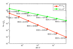
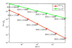
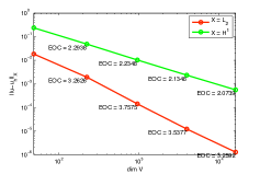
We discretize the problem given by (4.2) under the algorithm set out in §2.2, numerical convergence results are shown in Figure 2.

4.2. Test problem with convection dominated operator

The second test problem demonstrates the ability to overcome oscillations introduced into the standard finite element when rewriting the operator in divergence form. Take

$$a(\boldsymbol{x})=\operatorname{arctan}\left(K(\left|\boldsymbol{x}\right|^{2}-1)\right)+2$$ (4.5)

$$b(\boldsymbol{x})=0.$$ (4.6)

with $K\in\mathbb{R}^{+}$. Rewriting in divergence form gives

$${\boldsymbol{A}}{:}{\mathrm{D}^{2}u}=\operatorname{div}\left(\boldsymbol{A}\nabla u\right)-\operatorname{div}\left(\boldsymbol{A}\right)\nabla u.$$ (4.7)

The derivatives

$$\partial_{\alpha}{a}(\boldsymbol{x})=\frac{dKx_{\alpha}}{1+K\left(\left|\boldsymbol{x}\right|^{2}-1\right)}$$ (4.8)

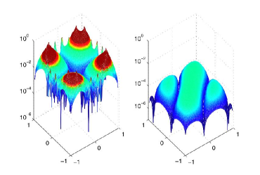
can be made arbitrarily large on the unit circle by choosing $K$ appropriately (see Figure  2(b)).

We choose our problem data $f$ such that the exact solution to the problem is given by:

$$u(\boldsymbol{x})=\operatorname{sin}\left(\pi x_{1}\right)\operatorname{sin}\left(\pi x_{2}\right).$$ (4.9)

We then construct the standard finite element method around (4.7), that is find $U\in\mathring{\mathbb{V}}$ such that for each $\mathring{\Phi}\in\mathring{\mathbb{V}}$

$$\left\langle\boldsymbol{A}\nabla U,\nabla\mathring{\Phi}\right\rangle-\left\langle\operatorname{div}\left(\boldsymbol{A}\right)\nabla U,\mathring{\Phi}\right\rangle=\left\langle f,\mathring{\Phi}\right\rangle.$$ (4.10)

If $K$ is chosen small enough the standard finite element method converges optimally. If we increase the value of $K$ oscillations become apparent in the finite element solution along the unit circle. Figure 4 demonstrates the oscillations arising from this method compared to discretizing using the nonvariational finite element method.

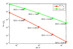
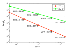
Figure 3 shows the numerical convergence rates of the nonvariational finite element method applied to this problem.

4.3. Test problem choosing a solution with nonsymmetric Hessian

In this test we choose the operator such that $b(\boldsymbol{x})$ is non-zero. To maintain ellipticity in this problem we must choose $a(\boldsymbol{x})$ such that the trace of $\boldsymbol{A}$ dominates it’s determinant. We choose

$$a(\boldsymbol{x})=2$$ (4.11)

$$b(\boldsymbol{x})=(x_{1}^{2}x_{2}^{2})^{1/3}.$$ (4.12)

We choose the problem data such that the exact solution is given by

$$u(\boldsymbol{x})=\begin{cases}\frac{x_{1}x_{2}(x_{1}^{2}-x_{2}^{2})}{x_{1}^{2}+x_{2}^{2}}&\boldsymbol{x}\neq\boldsymbol{0}\\ 0&\boldsymbol{x}=\boldsymbol{0}.\end{cases}$$ (4.13)

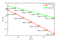
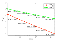
This function has a nonsymmetric Hessian at the point $\boldsymbol{0}$. The nontrivial Dirichlet boundary is dealt with using Remark 3.6. Figure 5 shows numerical results for this problem.

4.4. Test problem with quasilinear PDE in nondivergence form

The problem under consideration in this test is the following quasi-linear PDE arising from differential geometry:

$$\operatorname{div}\left(\frac{\nabla u}{\sqrt{1+\left|\nabla u\right|^{2}}}\right)=\frac{f}{\sqrt{1+\left|\nabla u\right|^{2}}},$$ (4.14)

where $\sqrt{1+\left|\nabla u\right|^{2}}$ is the area element. Here we are using $\left|\nabla u\right|^{2}=\mathrm{D}u\nabla u$. Applying a fixed point linearization given an initial guess $u^{0}$ for each $n\in\mathbb{N}$ we seek $u^{n}$ such that

$$\operatorname{div}\left(\frac{\nabla u^{n}}{\sqrt{1+\left|\nabla u^{n-1}\right|^{2}}}\right)=\frac{f}{\sqrt{1+\left|\nabla u^{n-1}\right|^{2}}}.$$ (4.15)

Applying a standard finite element discretization of (4.15) yields: Given $U^{0}\in\mathring{\mathbb{V}}$, for each $n\in\mathbb{N}$ find $U^{n}\in\mathring{\mathbb{V}}$ such that for each $\mathring{\Phi}\in\mathring{\mathbb{V}}$

$$\left\langle{\frac{\nabla U^{n}}{\sqrt{1+\left|\nabla U^{n-1}\right|^{2}}}},\nabla\mathring{\Phi}\right\rangle=\left\langle\frac{f}{\sqrt{1+\left|\nabla U^{n-1}\right|^{2}}},\mathring{\Phi}\right\rangle.$$ (4.16)

In fact we can work on this problem combining the two nonlinear terms. To do so we must first rewrite (4.14) into the form ${A(u,\nabla u)}{:}{\mathrm{D}^{2}u}=f$.

$$\begin{split}f=&\sqrt{1+\left|\nabla u\right|^{2}}\operatorname{div}\left(\frac{\nabla u}{\sqrt{1+\left|\nabla u\right|^{2}}}\right)\\ =&\sqrt{1+\left|\nabla u\right|^{2}}\left(\frac{\Delta u}{\sqrt{1+\left|\nabla u\right|^{2}}}+\frac{\mathrm{D}\left(1+\left|\nabla u\right|^{2}\right)}{2\left(1+\left|\nabla u\right|^{2}\right)^{3/2}}\nabla u\right)\\ =&\Delta u+\frac{\mathrm{D}u\mathrm{D}^{2}u\nabla u}{1+\left|\nabla u\right|^{2}}\\ =&{\left(\boldsymbol{I}+\frac{\nabla u\mathrm{D}u}{1+\left|\nabla u\right|^{2}}\right)}{:}{\mathrm{D}^{2}u}.\end{split}$$ (4.17)

Applying a similar fixed point linearization given an initial guess $u^{0}$ for each $n\in\mathbb{N}$ we seek $u^{n}$ such that

$${\left(\boldsymbol{I}+\frac{\nabla u^{n-1}\mathrm{D}u^{n-1}}{1+\left|\nabla u^{n-1}\right|^{2}}\right)}{:}{\mathrm{D}^{2}u^{n}}=f$$ (4.18)

Discretizing the problem is then similar to that set out in Section 2.2. The component matrixes ${\boldsymbol{\mathsf{M}}}$ and ${\boldsymbol{\mathsf{C}}}_{\alpha,\beta}$ are problem independent, ${\boldsymbol{\mathsf{B}}}^{\alpha,\beta}$ are defined as

$${\boldsymbol{\mathsf{B}}}^{\alpha,\beta}=\begin{cases}\left\langle{\boldsymbol{\mathsf{\mathring{\Phi}}}},1+\frac{\partial_{\alpha}{U}^{n-1}\partial_{\beta}{U}^{n-1}}{1+\left|\nabla U^{n-1}\right|^{2}}{\boldsymbol{\mathsf{\Phi}}}\right\rangle,&\text{ for }\alpha=\beta,\\ \\ \left\langle{\boldsymbol{\mathsf{\mathring{\Phi}}}},\frac{\partial_{\alpha}{U}^{n-1}\partial_{\beta}{U}^{n-1}}{1+\left|\nabla U^{n-1}\right|^{2}}{\boldsymbol{\mathsf{\Phi}}}\right\rangle,&\text{ for }\alpha\neq\beta.\end{cases}$$ (4.19)

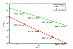
Table 2 compares the two linearizations (4.15) and (4.18). Figure 6 show asymptotic numerical convergence results for NVFEM applied to (4.18).

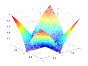
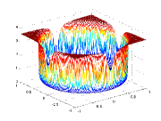
Figure 1. A visualization of the coefficient of the operators (4.2) (on the left) and (4.5) (on the right).

(a) The function $(x_{1}^{2}x_{2}^{2})^{1/3}+1$ over $\varOmega$. Note the derivatives are singular at $x_{1}=0$ and $x_{2}=0$.

(b) The function $\operatorname{arctan}\left(5000(\left|x\right|^{2}-1)\right)$ over $\varOmega$. Note the derivatives are very large on the unit circle.

Figure 2. Test 4.1. Errors and convergence rates for the NVFEM applied to a non-divergence form operator (4.2), choosing $f$ appropriately such that $u(\boldsymbol{x})=\exp{(-10\left|\boldsymbol{x}\right|)}$. The convergence rates are optimal, that is for $\mathbb{P}^{1}$-elements (on the left) $\left\|u-U\right\|=\operatorname{O}(h^{2})$ and $\left|u-U\right|_{1}=\operatorname{O}(h)$. For $\mathbb{P}^{2}$-elements (on the right) $\left\|u-U\right\|=\operatorname{O}(h^{3})$ and $\left|u-U\right|_{1}=\operatorname{O}(h^{2})$.

(a) $\mathbb{P}^{1}$-elements

(b) $\mathbb{P}^{2}$-elements

Table 1. Test 4.1. On the condition number of ${\boldsymbol{\mathsf{E}}}$ upon discretizing problem (4.2) using $\mathbb{P}^{1}$ finite elements. As claimed in Remark 3.8 $\kappa({\boldsymbol{\mathsf{E}}})\approx Ch^{-2}$.

$\dim{\mathbb{V}}$	$h$	$\kappa({\boldsymbol{\mathsf{E}}})$	$h^{-2}\kappa({\boldsymbol{\mathsf{E}}})$
$16$	$0.4714$	$4.904\times 10^{1}$	$10.898$
$64$	$0.202$	$6.594\times 10^{2}$	$26.952$
$256$	$0.0943$	$3.665\times 10^{3}$	$32.633$
$1024$	$0.0456$	$1.722\times 10^{4}$	$35.833$
$4096$	$0.0224$	$6.894\times 10^{4}$	$34.737$
$16384$	$0.0111$	$3.383\times 10^{5}$	$41.949$
$65536$	$0.0055$	$1.337\times 10^{6}$	$40.43$

Figure 3. Test 4.2. Errors and convergence rates for the NVFEM applied to a non-divergence form operator (4.5) with $K=5000$, choosing $f$ appropriately such that $u(\boldsymbol{x})=\operatorname{sin}\left(\pi x_{1}\right)\operatorname{sin}\left(\pi x_{2}\right)$. The convergence rates are optimal, that is for $\mathbb{P}^{1}$-elements (on the left) $\left\|u-U\right\|=\operatorname{O}(h^{2})$ and $\left|u-U\right|_{1}=\operatorname{O}(h)$. For $\mathbb{P}^{2}$-elements (on the right) $\left\|u-U\right\|=\operatorname{O}(h^{3})$ and $\left|u-U\right|_{1}=\operatorname{O}(h^{2})$.

(a) $\mathbb{P}^{1}$-elements

(b) $\mathbb{P}^{2}$-elements

Figure 4. Test 4.2. On the left we present $\smash{\left\|u-\tilde{U}\right\|}_{\operatorname{L}_{\infty}(K)}$ plotted on a logarithmic scale as a function over $\varOmega$. This represents the maximum error of the standard FE-solution, $\tilde{U}$, to problem (4.5) with $16384$ DOF’s ($h=1/32$). Notice the oscillations apparent on the unit circle. On the right we show $\left\|u-{U}\right\|_{\operatorname{L}_{\infty}(K)}$ plotted on a logarithmic scale as a function over $\varOmega$, the maximum error of the NVFE-solution, $U$, to problem (4.5) with $16384$ DOF’s ($h=1/32$).

Figure 5. Test 4.3. Errors and convergence rates for the NVFEM on an operator (4.11), choosing $f$ appropriately such that $u(\boldsymbol{x})=\frac{x_{1}x_{2}(x_{1}^{2}-x_{2}^{2})}{x_{1}^{2}+x_{2}^{2}}$ if $\boldsymbol{x}\neq\boldsymbol{0}$, or $u(\boldsymbol{x})=0$ otherwise. The convergence rates are optimal, that is for $\mathbb{P}^{1}$-elements (on the left) $\left\|u-U\right\|=\operatorname{O}(h^{2})$ and $\left|u-U\right|_{1}=\operatorname{O}(h)$. For $\mathbb{P}^{2}$-elements (on the right) $\left\|u-U\right\|=\operatorname{O}(h^{3})$ and $\left|u-U\right|_{1}=\operatorname{O}(h^{2})$.

(a) $\mathbb{P}^{1}$-elements

(b) $\mathbb{P}^{2}$-elements

Table 2. Test 4.4. Comparison of the fixed point linearization in variational form (4.15) and in nonvariational form (4.18). We fix $f$ appropriately such that $u(\boldsymbol{x})=\operatorname{sin}\left(\pi x_{1}\right)\operatorname{sin}\left(\pi x_{2}\right)$. Taking initial guesses $U^{0}=\tilde{U^{0}}=0$ we discretize problem (4.14) using a standard FEM and using the NVFEM. Denoting $U_{i}$ and $\tilde{U}_{i}$ to be the NVFE-solution FE-solution respectively we run both linearizations for until a tolerance $\left\|U_{n+1}-U_{n}\right\|$ (resp. $\smash{\left\|\tilde{U}_{n+1}-\tilde{U}_{n}\right\|}$) $\leq h^{2}$ is achieved. We compute both the stagnation point—which is the iteration at which the prescribed tolerance is achieved—and the total CPU time. Notice there is significant savings in the number of iterations required to reach the stagnation point using the NVFEM over the standard FEM, however each iteration is computationally more costly using the NVFEM since the system is larger and more complicated to solve. The CPU cost for the entire algorithm is comparable for each fixed $h$.

	$h$	$\sqrt{2}/5$	$\sqrt{2}/10$	$\sqrt{2}/20$	$\sqrt{2}/40$	$\sqrt{2}/80$	$\sqrt{2}/160$
FEM	Stag. Point	$5$	$13$	$16$	$26$	$32$	$36$
	CPU Time	$0.50$	$4.02$	$17.51$	$117.58$	$796.58$	$5308.81$
NDFEM	Stag. Point	$4$	$6$	$7$	$8$	$10$	$12$
	CPU Time	$0.72$	$3.40$	$16.49$	$97.93$	$838.8$	$5256.84$

Figure 6. Test 4.4. Errors and convergence rates for NVFEM applied to (4.14), a quasi-linear PDE under a fixed point linearization. We fix $f$ appropriately such that $u(\boldsymbol{x})=\operatorname{sin}\left(\pi x_{1}\right)\operatorname{sin}\left(\pi x_{2}\right)$, taking an initial guess $u^{0}=0$. The convergence rates are optimal, that is for $\mathbb{P}^{1}$-elements (on the left) $\left\|u-U\right\|=\operatorname{O}(h^{2})$ and $\left|u-U\right|_{1}=\operatorname{O}(h)$. For $\mathbb{P}^{2}$-elements (on the right) $\left\|u-U\right\|=\operatorname{O}(h^{3})$ and $\left|u-U\right|_{1}=\operatorname{O}(h^{2})$.

(a) $\mathbb{P}^{1}$-elements

(b) $\mathbb{P}^{2}$-elements

References

• [AM08] Néstor E. Aguilera and Pedro Morin. On convex functions and the finite element method. online preprint arXiv:0804.1780v1, arXiv.org, Apr 2008.
• [AV02] A. Agouzal and Yu. Vassilevski. On a discrete Hessian recovery for P1subscript𝑃1P_{1} finite elements. J. Numer. Math., 10(1):1–12, 2002.
• [Böh08] Klaus Böhmer. On finite element methods for fully nonlinear elliptic equations of second order. SIAM J. Numer. Anal., 46(3):1212–1249, 2008.
• [Cia78] Philippe G. Ciarlet. The finite element method for elliptic problems. North-Holland Publishing Co., Amsterdam, 1978. Studies in Mathematics and its Applications, Vol. 4.
• [CS08] Luis A. Caffarelli and Panagiotis E. Souganidis. A rate of convergence for monotone finite difference approximations to fully nonlinear, uniformly elliptic PDEs. Comm. Pure Appl. Math., 61(1):1–17, 2008.
• [CSX07] Long Chen, Pengtao Sun, and Jinchao Xu. Optimal anisotropic meshes for minimizing interpolation errors in Lpsuperscript𝐿𝑝L^{p}-norm. Math. Comp., 76(257):179–204 (electronic), 2007.
• [Eva98] Lawrence C. Evans. Partial differential equations, volume 19 of Graduate Studies in Mathematics. American Mathematical Society, Providence, RI, 1998.
• [GT83] David Gilbarg and Neil S. Trudinger. Elliptic Partial Differential Equations of Second Order. Springer-Verlag, Berlin, second edition, 1983.
• [KT92] Hung Ju Kuo and Neil S. Trudinger. Discrete methods for fully nonlinear elliptic equations. SIAM J. Numer. Anal., 29(1):123–135, 1992.
• [LR05] Grégoire Loeper and Francesca Rapetti. Numerical solution of the Monge-Ampère equation by a Newton’s algorithm. C. R. Math. Acad. Sci. Paris, 340(4):319–324, 2005.
• [Obe08] Adam M. Oberman. Wide stencil finite difference schemes for the elliptic Monge-Ampère equation and functions of the eigenvalues of the Hessian. Discrete Contin. Dyn. Syst. Ser. B, 10(1):221–238, 2008.
• [Tho06] Vidar Thomée. Galerkin finite element methods for parabolic problems, volume 25 of Springer Series in Computational Mathematics. Springer-Verlag, Berlin, second edition, 2006.
• [VMD+07] M.-G. Vallet, C.-M. Manole, J. Dompierre, S. Dufour, and F. Guibault. Numerical comparison of some Hessian recovery techniques. Internat. J. Numer. Methods Engrg., 72(8):987–1007, 2007.