Power Counting Regime of Chiral Effective Field Theory and Beyond

Abstract

Chiral effective field theory ($\chi$EFT) complements numerical simulations of quantum chromodynamics (QCD) on a space-time lattice. It provides a model-independent formalism for connecting lattice simulation results at finite volume and a variety of quark masses to the physical world. The asymptotic nature of the chiral expansion places the focus on the first few terms of the expansion. Thus, knowledge of the power-counting regime (PCR) of $\chi$EFT, where higher-order terms of the expansion may be regarded as negligible, is as important as knowledge of the expansion itself. Through the consideration of a variety of renormalization schemes and associated parameters, techniques to identify the PCR where results are independent of the renormalization scheme are established. The nucleon mass is considered as a benchmark for illustrating this general approach. Because the PCR is small, the numerical simulation results are also examined to search for the possible presence of an intrinsic scale which may be used in a nonperturbative manner to describe lattice simulation results outside of the PCR. Positive results that improve on the current optimistic application of chiral perturbation theory ($\chi$PT) beyond the PCR are reported.

I Introduction

The low energy chiral effective field theory ($\chi$EFT) of quantum chromodynamics (QCD) provides a model-independent approach for understanding the consequences of dynamical chiral-symmetry breaking in the chiral properties of hadrons. Non-analytic contributions in the quark mass are generated by the pseudo-Goldstone meson dressings of hadrons through meson-loop integrals. Chiral perturbation theory ($\chi$PT) provides a formal approach to counting the powers of low energy momenta and quark masses such that an ordered expansion in powers of the quark mass $m_{q}\propto m_{\pi}^{2}$ is constructed. $\chi$PT indicates that, in general, the most singular nonanalytic contributions to hadron properties lie in the one-loop ‘meson cloud’ of the hadron. For example, the leading nonanalytic behavior of a baryon mass is proportional to $m_{q}^{3/2}$ or $m_{\pi}^{3}$. More generally, baryon masses can be written as an ordered expansion in quark mass or $m_{\pi}^{2}$.

To establish a model-independent framework in $\chi$PT, the expansion must display the properties of a convergent series for the terms considered. There is a power-counting regime (PCR) where the quark mass is small, and higher-order terms in the expansion are negligible beyond the order calculated. Within the PCR, the truncation of the chiral expansion is reliable to a prescribed precision.

The asymptotic nature of the chiral expansion places the focus on the first few terms of the expansion. A survey of the literature for the baryon sector of $\chi$EFT illustrates the rarity of calculations beyond one-loop McGovern and Birse (1999, 2006); Schindler et al. (2007), and there are no two-loop calculations which incorporate the effects of placing a baryon in a finite volume. With only a few terms of the expansion known for certain, knowledge of the PCR of $\chi$EFT is as important as knowledge of the expansion itself. It is within the PCR that higher-order terms of the expansion may be regarded as negligible.

Numerical simulations of QCD on a space-time lattice are complemented by $\chi$EFT through the provision of a model-independent formalism for connecting lattice simulation results to the physical world. Simulations at finite volume and a variety of quark masses are related to the infinite volume and physical quark masses through this formalism. However, the formalism is accurate only if one works within the PCR of the truncated expansion. Present practice in the field is best described as optimistic. Truncated expansions are regularly applied to a wide range of quark (or pion) masses with little regard to a rigorous determination of the PCR.

When considering nucleons, there is some evidence that the PCR may be quite small; constrained by $m_{\pi}\lesssim 200$ MeV at $1\%$ accuracy at the chiral order $\mathcal{O}(m_{\pi}^{4}\,\log m_{\pi})$ Beane (2004a) Leinweber et al. (2005a). This estimate of the PCR of $\chi$PT was identified using specific finite-range regularization (FRR) techniques to analyze lattice QCD data. Using FRR, the regime is manifest when the quark-mass dependence of the nucleon mass is independent of the renormalization scheme parameter.

A chief focus of this paper is to establish a rigorous approach to determining the PCR of a truncated chiral expansion quantitatively. Through the consideration of a variety of renormalization schemes and associated parameters, new techniques to identify the PCR are established. The PCR is the regime where results are scheme independent. The nucleon mass is considered as a benchmark for illustrating this general approach. Here, the chiral expansion is examined, focusing on the individual low energy coefficients of the chiral expansion. This approach provides a determination of the PCR for a truncated expansion in $\chi$EFT. As discussed in detail in the following section, the PCR is indeed small for the nucleon mass. Other observables are expected to show a similar if not smaller PCR. Thus most of today’s lattice simulation results lie outside the PCR, and the truncated chiral expansions have been used to extrapolate from outside the PCR. The low energy coefficients determined by applying the truncated expansion outside the PCR will take on unphysical values, as they accommodate important but otherwise missing contributions from non-negligible higher-order terms.

While continued advances in numerical simulations of lattice QCD will be vital to some extent in resolving this problem, the physical value of the strange-quark mass presents a challenge that will not diminish with supercomputing advances. If one were to include the effects of kaons, vital to understanding strangeness in the nucleon for example, then one must either calculate to significantly higher order in the expansion of $\chi$PT, or develop new non-perturbative approaches which utilize the non-perturbative information expressed in the lattice simulation results. Since the former is likely to be compromised by the asymptotic nature of the expansion, attention is given to the latter approach.

Thus the second focus of this paper is to examine the numerical simulation results, to identify the possible presence of an intrinsic scale. This may then be used to address lattice simulation results outside of the PCR in a non-perturbative manner. Of course, the non-perturbative formalism must incorporate the exact perturbative results of $\chi$PT in the PCR. Positive results are reported that improve on the current optimistic application of $\chi$PT outside of the PCR.

The outline of the presentation is as follows. Sec. II reviews chiral effective field theory and the process of regularization and renormalization. The adoption of finite-range regularization (FRR) provides a wide range of schemes and scales, which overlap with the more popular massless renormalization schemes as the finite-range regulator parameter is taken to infinity. Sec. III investigates FRR in the context of a particular model. By generating a set of pseudodata and analysing it with a variety of renormalization schemes, a robust method for determining the PCR is obtained, along with an optimal renormalization scale to use beyond the PCR. Finally, Sec. IV includes the analysis of three sets of lattice results for the nucleon mass, utilizing the tools developed in the previous section. Conclusions are summarized in Sec. V.

II Effective Field Theory

This section begins by briefly reviewing the process of regularization and renormalization in finite-range regularized (FRR) chiral effective field theory, providing a range of renormalization schemes and scales. A central focus is to search for the dependence of physical results on the scheme and associated scales, as these will be an indication that one is applying the chiral expansion outside the PCR.

The focus is to establish techniques that provide a quantitative test of whether a given range of $m_{\pi}$ lies within the PCR. This is achieved through an examination of the flow of the low energy coefficients as a function of the renormalization scheme parameter(s). A negligible dependence would confirm that the pion-mass range is within the PCR. On the other hand, the properties of the flow will be used to identify a preferred regularization scheme in a non-perturbative sense that best describes the results beyond the PCR.

II.1 Renormalization in FRR $\chi$EFT

Using the standard Gell-Mann–Oakes–Renner relation connecting quark and pion masses, $m_{q}\propto m_{\pi}^{2}$ Gell-Mann et al. (1968), the formal chiral expansion of the nucleon can be written as a polynomial expansion in $m_{\pi}^{2}$ plus the meson-loop integral contributions:

$$M_{N} = \{a_{0}+a_{2}m_{\pi}^{2}+a_{4}m_{\pi}^{4}+\mathcal{O}(m_{\pi}^{6})\}$$ (1)

$$+ \Sigma_{N}+\Sigma_{\Delta}+\Sigma_{tad}\,.$$

The pion cloud corrections are considered in the heavy-baryon limit, with loop integrals, $\Sigma_{N}$, $\Sigma_{\Delta}$ and $\Sigma_{tad}$, corresponding to Figures 3 through 3, respectively. The coefficients $a_{i}$ of the analytic polynomial, contained in brackets $\{\,\}$ in Eq. (1), are related to the low energy constants of $\chi$PT. In this investigation, they will be determined by fitting to lattice QCD data. These coefficients will be referred to as the residual series coefficients. These bare coefficients undergo renormalization due to contributions from the loop integrals $\Sigma_{N}$, $\Sigma_{\Delta}$ and $\Sigma_{tad}$.

Under the most general considerations, each loop integral, when evaluated, produces an analytic polynomial in $m_{\pi}^{2}$ and nonanalytic terms:

$$\Sigma_{N} = b_{0}^{N}+b_{2}^{N}m_{\pi}^{2}+\chi_{N}m_{\pi}^{3}+b_{4}^{N}m_{\pi}^{4}+\mathcal{O}(m_{\pi}^{5})\,,$$ (2)

$$\Sigma_{\Delta} = b_{0}^{\Delta}+b_{2}^{\Delta}m_{\pi}^{2}+b_{4}^{\Delta}m_{\pi}^{4}$$ (3)

$$+\frac{3}{4\pi\Delta}\chi_{\Delta}m_{\pi}^{4}\,\log\frac{m_{\pi}}{\mu}+\mathcal{O}(m_{\pi}^{5})\,,$$

$$\Sigma_{tad} = b_{2}^{t^{\prime}}m_{\pi}^{2}+b_{4}^{t^{\prime}}m_{\pi}^{4}+\chi_{t}^{\prime}m_{\pi}^{4}\,\log\frac{m_{\pi}}{\mu}+\mathcal{O}(m_{\pi}^{5}).$$ (4)

Here $\Delta$ is the delta-nucleon mass splitting in the chiral limit, taken to be $292$ MeV. $\chi_{N}$, $\chi_{\Delta}$ and $\chi_{t}^{\prime}$ denote the model independent chiral coefficients of the terms that are nonanalytic in the quark mass. The $b_{i}$ coefficients are renormalization scheme dependent as are the $a_{i}$ coefficients. It can be noted that the tadpole loop contribution $\Sigma_{tad}$ does not produce a $b_{0}^{t}$ term because it enters with a leading factor of $m_{\pi}^{2}$, as discussed in Section II.2. The primes on the coefficients $b_{2}^{t^{\prime}}$ and $\chi_{t}^{\prime}$ here simply indicate that they will be used later in a slightly different form.

The process of renormalization in FRR $\chi$EFT proceeds by combining the renormalization-scheme dependent coefficients to provide the physical low energy coefficients, which are denoted as $c_{i}$. Thus, the nucleon mass expansion takes on the standard form:

$$M_{N} = c_{0}+c_{2}m_{\pi}^{2}+\chi_{N}m_{\pi}^{3}+c_{4}m_{\pi}^{4}$$ (5)

$$+ \!\left(\!\!-\frac{3}{4\pi\Delta}\chi_{\Delta}+c_{2}\chi_{t}\!\right)\!m_{\pi}^{4}\log\frac{m_{\pi}}{\mu}+\mathcal{O}(m_{\pi}^{5})\,.$$

By comparing Eqs. (1) through (5), the following renormalization procedure is obtained:

$$c_{0} = a_{0}+b_{0}^{N}+b_{0}^{\Delta}\,,$$ (6)

$$c_{2} = a_{2}+b_{2}^{N}+b_{2}^{\Delta}+b_{2}^{t^{\prime}}\,,$$ (7)

$$c_{4} = a_{4}+b_{4}^{N}+b_{4}^{\Delta}+b_{4}^{t^{\prime}}\,,\mbox{\,\,etc.}$$ (8)

The coefficients $c_{i}$ are scheme independent quantities, and this property will be demonstrated when determined within the PCR. The value of $c_{0}$ is the nucleon mass in the chiral limit ($m_{\pi}^{2}=0$), and $c_{2}$ is related to the so-called sigma term of explicit chiral symmetry breaking Leinweber et al. (2000); Wright et al. (2000); Holl et al. (2006). The nonanalytic terms $m_{\pi}^{3}$ and $m_{\pi}^{4}\,\log m_{\pi}/\mu$ have known, constant coefficients denoted by $\chi_{N}$, $\chi_{\Delta}$ and $\chi_{t}$. The value of $c_{4}$ is scale dependent, such that the total $m_{\pi}^{4}$ term in Eq. (5), including the logarithm, is independent of the scale $\mu$. It can be noted that the nucleon mass itself is completely independent of the choice of $\mu$. For the numerical analysis, $\mu$ is set equal to $1\,{\rm GeV}$.

Figure 1: The pion loop contribution to the self-energy of the nucleon, providing the leading nonanalytic contribution to the nucleon mass. All charge conserving transitions are implicit.

Figure 2: The pion loop contribution to the self-energy of the nucleon allowing transitions to the near-by and strongly-coupled decuplet baryons.

Figure 3: Tadpole contributions to the nucleon self energy.

Of course, EFT loop calculations are commonly divergent without some regularization method. Since the effective field theory is only applicable for low energies, hard momenta contributions to loop calculations may be eliminated. However, the traditional schemes including dimensional regularization (DR) often do not involve an explicit scale dependence when evaluating loop diagrams. Without any momentum cutoff, the $b_{i}$ coefficients from each loop integral become either infinite or vanish, and the $c_{i}$ coefficients from Eq. (5) undergo an infinite renormalization or none at all:

$$c_{0} = a_{0}-\infty\,,$$ (9)

$$c_{2} = a_{2}+\infty\,,$$ (10)

$$c_{4} = a_{4}+0\,,\mbox{\,\,etc.}$$ (11)

Since the $c_{i}$ coefficients are finite after renormalization, the $a_{i}$ coefficients must have been infinite, with the opposite sign of the $b_{i}$ coefficients. As emphasized above, both the $a_{i}$ and $b_{i}$ coefficients are scheme dependent. The infinities are absorbed in constructing the $c_{i}$ coefficients and thus subtracted from the chiral expansion. This minimal subtraction scheme with no explicit scale dependence makes DR quite suitable for elementary fields, where the absence of new degrees of freedom at higher energies is assumed. However, for EFTs there is an energy scale beyond which the effective fields are no longer the relevant degrees of freedom. When one integrates loop contributions over this high energy domain, there is no guarantee that one can efficiently subtract the model-dependent, ultraviolet physics with a finite number of counter-terms (unless in the PCR). As a result, the chiral expansion typically only shows reliable convergence properties over a narrow range of pion mass.

Indeed this problem of beginning with rapidly varying loop contributions, which must then be removed with a finite number of counter-terms, can easily be overcome. The hard momentum contributions to the meson-loop diagrams can be suppressed via the introduction of a regulator. As such, the coefficients of the residual expansion are likely to be smaller, and the utility of the expansion has the potential to apply to a broader range of quark or pion masses. The introduction of a regulator acts to resum the chiral expansion, with loop integrals having the general properties described in Eqs. (2) through (4).

The resummation of the chiral series through the introduction of a regulator (or similar variant) has been studied in various instances Donoghue et al. (1999); Young et al. (2002, 2003); Borasoy et al. (2002); Leinweber et al. (2004); Bernard et al. (2004); Djukanovic et al. (2005); Young et al. (2005); Leinweber et al. (2005b, a). The method consists of inserting a regulator function $u(k^{2})$ into the integrand of the meson-loop integrals. The regulator can take any form, so long as it is normalized to $1$, and approaches $0$ sufficiently fast to ensure convergence of the loop. Unlike DR, this method involves an explicit momentum cutoff scale, $\Lambda$. The chiral expansion can now be written in terms of this cutoff scale:

$$M_{N} = \{a_{0}^{\Lambda}+a_{2}^{\Lambda}\,m_{\pi}^{2}+a_{4}^{\Lambda}\,m_{\pi}^{4}+\mathcal{O}(m_{\pi}^{6})\}$$ (12)

$$+ \Sigma_{N}(m_{\pi}^{2},\Lambda)+\Sigma_{\Delta}(m_{\pi}^{2},\Lambda)+\Sigma_{tad}(m_{\pi}^{2},\Lambda).\,\,$$

The superscript $\Lambda$ denotes the scheme dependence of the $a_{i}^{\Lambda}$ coefficients. The loop integrals are functions of the scale $\Lambda$ and also $m_{\pi}^{2}$.

Through the introduction of the regulator, the loop integrals are now low energy contributions, significant for small $m_{\pi}^{2}$ and becoming negligible as $m_{\pi}^{2}$ becomes large. The scheme dependent $a_{i}^{\Lambda}$ coefficients undergo a renormalization, as before, via their combination with the $b_{i}^{\Lambda}$ coefficients, whose scheme dependence is now explicit, reflecting the regularization of the loop integrals:

$$c_{0} = a_{0}^{\Lambda}+b_{0}^{\Lambda,N}+b_{0}^{\Lambda,\Delta}\,,$$ (13)

$$c_{2} = a_{2}^{\Lambda}+b_{2}^{\Lambda,N}+b_{2}^{\Lambda,\Delta}+b_{2}^{\Lambda,t^{\prime}}\,,$$ (14)

$$c_{4} = a_{4}^{\Lambda}+b_{4}^{\Lambda,N}+b_{4}^{\Lambda,\Delta}+b_{4}^{\Lambda,t^{\prime}}\,,\mbox{\,\,etc.}$$ (15)

Dimensional analysis reveals that the coefficients $b_{i}$ are proportional to $\Lambda^{(3-i)}$. Thus it can be realized that as the cutoff scale $\Lambda$ goes to infinity the FRR expansion reduces to that of Eq. (5) via Eqs. (9) through (11). At any finite $\Lambda$, a partial resummation of higher-order terms is introduced.

Previous studies indicate that extrapolation results show very little sensitivity to the precise functional form of the regulator Leinweber et al. (2004). In this investigation, the family of smoothly attenuating dipole regulators will be considered. The general $n-$tuple dipole function takes the following form, for a cutoff scale of $\Lambda$:

$$u_{n}(k^{2})={\left(1+{\frac{k^{2n}}{\Lambda^{2n}}}\right)}^{-2}\,.$$ (16)

The standard dipole is recovered for $n=1$. The cases $n=2,3$ are the ‘double-’ and ‘triple-dipole’ regulators, respectively. In the following, $u(k^{2})$ is used to denote one of these regulators. This functional form allows one to interpolate between the dipole regulator and the step function (which corresponds to $n\to\infty$).

In a study by Bernard et al. Bernard et al. (2004), it was suggested that only a sharp cutoff FRR scheme is consistent with chiral symmetry. Djukanovic et al. Djukanovic et al. (2005) have demonstrated more general functional forms can be generated by proposing a scheme in which the regulator function is interpreted as a modification to the propagators of the theory, obtained from a new chiral symmetry-preserving Lagrangian. Higher-derivative coupling terms are built into the Lagrangian in order to produce a regulator from the Feynman Rules in a symmetry preserving manner.

The regulators used in the present investigation are introduced in a less systematic fashion, such that chiral symmetry is not automatically preserved to the order calculated. The higher derivative couplings of the regulator induces scheme-dependent nonanalytic terms. To maintain chiral symmetry, one must introduce the necessary vertex corrections.

Alternatively, one can choose the regulator judiciously such that any extra scheme-dependent nonanalytic are removed to any chosen order. For example, the $n-$tuple dipole regulators generate extra nonanalytic terms in the chiral expansion of Eq. (5) at higher chiral orders. For a dipole regulator, regulator-dependent nonanalytic terms occur at odd powers of $m_{\pi}$, beginning at $\mathcal{O}(m_{\pi}^{5})$ . In the case of the double dipole, the nonanalytic terms begin at $\mathcal{O}(m_{\pi}^{7})$, and for the triple dipole the nonanalytic terms begin only at $\mathcal{O}(m_{\pi}^{9})$.

In a final observation, it is essential to note that the degrees of freedom present in the residual series coefficients, $a_{i}^{\Lambda}$, are sufficient to eliminate any dependence on the regulator parameter, $\Lambda$, to the order of the chiral expansion calculated: in this case ${\cal O}(m_{\pi}^{4})$. By definition, higher order terms in the FRR expansion are negligible in the PCR, and therefore FRR $\chi$EFT is mathematically equivalent to $\chi$PT in the PCR. Any differences observed in results obtained at the same chiral order but with different regularization schemes are a direct result of considering data that lie outside the PCR (provided that the regulator $\Lambda$ is not chosen too small such as to introduce an unphysical low energy scale).

II.2 Loop Integrals and Definitions

The leading order loop integral contributions to the nucleon mass, corresponding to the diagrams in Figures 3 through 3, can be simplified to a convenient form by taking the heavy-baryon limit, and performing the pole integration for $k_{0}$. Renormalization, as outlined above, is achieved by subtracting the relevant terms in the Taylor expansion of the loop integrals and absorbing them into the corresponding low energy constants, $c_{i}$:

$$\tilde{\Sigma}_{N} = \chi_{N}\frac{1}{2\pi^{2}}\int\!\!\mathrm{d}^{3}k\frac{k^{2}u^{2}(k^{2})}{\omega^{2}(k)}-b_{0}^{\Lambda,N}-b_{2}^{\Lambda,N}m_{\pi}^{2}$$ (17)

$$= \chi_{N}m_{\pi}^{3}+b_{4}^{\Lambda,N}m_{\pi}^{4}+\mathcal{O}(m_{\pi}^{5})\,,$$ (18)

$$\tilde{\Sigma}_{\Delta} = \chi_{\Delta}\frac{1}{2\pi^{2}}\int\!\!\mathrm{d}^{3}k\frac{k^{2}u^{2}(k^{2})}{\omega(k)\left(\Delta+\omega(k)\right)}$$ (19)

$$\quad-b_{0}^{\Lambda,\Delta}-b_{2}^{\Lambda,\Delta}m_{\pi}^{2}$$

$$= b_{4}^{\Lambda,\Delta}m_{\pi}^{4}-\frac{3}{4\pi\Delta}\chi_{\Delta}m_{\pi}^{4}\,\log\frac{m_{\pi}}{\mu}+\mathcal{O}(m_{\pi}^{5})\,,\qquad$$ (20)

$$\tilde{\Sigma}_{tad} = c_{2}m_{\pi}^{2}\left(\chi_{t}\frac{1}{4\pi}\int\!\!\mathrm{d}^{3}k\frac{2u^{2}(k^{2})}{\omega(k)}-b_{2}^{\Lambda,t}\right)$$ (21)

$$= c_{2}m_{\pi}^{2}\left(b_{4}^{\Lambda,t}m_{\pi}^{2}+\chi_{t}m_{\pi}^{2}\,\log\frac{m_{\pi}}{\mu}+\mathcal{O}(m_{\pi}^{5})\right)\qquad$$ (22)

$$= c_{2}m_{\pi}^{2}\tilde{\sigma}_{tad}\,.$$ (23)

These integrals are expressed in terms of the pion energy, $\omega(k)=\sqrt{k^{2}+m_{\pi}^{2}}$. The tilde ($\,\tilde{\,}\,$) denotes that the integrals are written out in renormalized form to chiral order $\mathcal{O}(m_{\pi}^{2})$. As the $b_{i}$ coefficients are regulator and scale dependent, this subtraction removes this dependence. The coefficients $a_{0}$ and $a_{2}$ of the analytic terms in the chiral expansion in Eq. (5) are now automatically the renormalized coefficients $c_{0}$ and $c_{2}$. This is because the $b_{0}$ and $b_{2}$ terms in Eqs. (13) and (14) are removed in the subtraction. Note also that the tadpole amplitude in Eqs. (22) and (23) contains the renormalized $c_{2}$ in its coefficient. The interaction vertex in this diagram arises from expanding out the pion field in the leading quark mass insertion.

The constant coefficients $\chi_{N}$, $\chi_{\Delta}$ and $\chi_{t}$ for each integral are defined in terms of the pion decay constant, which is taken to be $f_{\pi}=93$ MeV, and the axial coupling parameters $D$, $F$ and $\mathcal{C}$ which couple the baryons to the pion field. The phenomenological values for these couplings are used, applying the $\mathrm{SU}(6)$ flavour-symmetry relations Jenkins (1992); Lebed (1995) to yield $\mathcal{C}=-2D$, $F=\frac{2}{3}D$ and the value $D=0.76$:

$$\chi_{N} = -\frac{3}{32\pi f_{\pi}^{2}}(D+F)^{2}\,,$$ (24)

$$\chi_{\Delta} = -\frac{3}{32\pi f_{\pi}^{2}}\frac{8}{9}\mathcal{C}^{2}\,,$$ (25)

$$\chi_{t} = -\frac{3}{16\pi^{2}f_{\pi}^{2}}\,.$$ (26)

With the renormalized integrals specified, the FRR modified version of the chiral expansion in Eq. (5) takes the form:

$$M_{N}=c_{0}+c_{2}m_{\pi}^{2}(1+{\tilde{\sigma}}_{tad})+a_{4}^{\Lambda}m_{\pi}^{4}+{\tilde{\Sigma}}_{N}+{\tilde{\Sigma}}_{\Delta}\,.\\$$ (27)

The $a_{4}^{\Lambda}$ term is left in unrenormalized form for simplicity. Indeed, the $b_{4}$ can be evaluated by expanding out corresponding loop integrals, such as in Ref. Young et al. (2003). However, the focus here is on the behaviour of $c_{0}$ and $c_{2}$.

Since the results of lattice simulations reflect the presence of discrete momentum values associated with the finite volume of the lattices, the formalism must also take into account these finite volume effects. In order to accommodate the effect of the finite volume, the continuous loop integrals occurring in the meson loop calculations in infinite volume are transformed into a sum over discrete momentum values. The difference between a loop sum and its corresponding loop integral is the finite volume correction, which should vanish for all integrals as $m_{\pi}L$ becomes large Beane (2004b).

While Eq. (27) is useful in describing the pion mass evolution of the nucleon mass, for the consideration of lattice QCD results, one also needs to incorporate corrections to allow for the finite-volume nature of the numerical simulations. As the pion is the lightest degree of freedom in the system, it is the leading order pion loop effects that are most sensitive to the periodic boundary conditions. The corrections can be determined by considering the transformation of each loop integral in Eqs. (17), (19) and (21), into a discrete sum for lattice volume $V=L_{x}L_{y}L_{z}$ Armour et al. (2006):

$$\int\!\!\mathrm{d}^{3}k\rightarrow\frac{{(2\pi)}^{3}}{L_{x}L_{y}L_{z}}\sum_{k_{x},k_{y},k_{z}}\,.$$ (28)

Each momentum component is quantized in units of $2\pi/L$, that is $k_{i}=n_{i}2\pi/L$ for integers $n_{i}$. The finite volume correction $\delta^{\mathrm{FVC}}$ can be written as the difference between the finite sum and the integral:

$$\delta^{\mathrm{FVC}}_{i}\!\!=\frac{\chi_{i}}{2\pi^{2}}\Big{[}\frac{{(2\pi)}^{3}}{L_{x}L_{y}L_{z}}\!\!\sum_{k_{x},k_{y},k_{z}}\!\!\!\!\!I_{i}(\vec{k},m_{\pi}^{2},\Lambda)\,-\int\!\!\mathrm{d}^{3}k\,\,I_{i}(\vec{k},m_{\pi}^{2},\Lambda)\Big{]},\quad$$ (29)

where $i=N,\Delta$, and the integrands are denoted $I_{i}(\vec{k},m_{\pi}^{2},\Lambda)$. By adding the relevant finite volume correction (FVC) to each loop contribution, the finite volume nucleon mass can be parameterized:

$$M_{N}^{V} = c_{0}+c_{2}m_{\pi}^{2}(1+{\tilde{\sigma}}_{tad})+a_{4}^{\Lambda}m_{\pi}^{4}$$ (30)

$$+ ({\tilde{\Sigma}}_{N}+\delta_{N}^{\mathrm{FVC}})+({\tilde{\Sigma}}_{\Delta}+\delta_{\Delta}^{\mathrm{FVC}})\,.$$

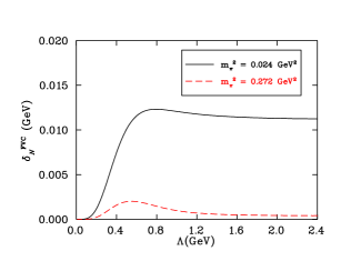
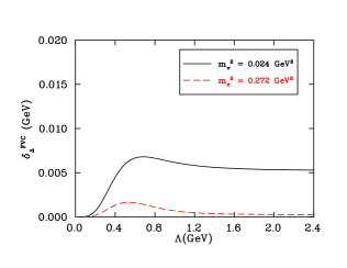
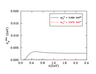
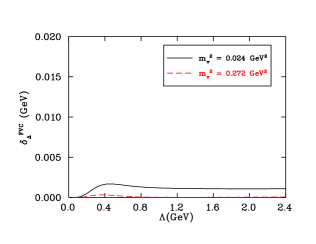
It is also anticipated that the FVC are independent of the regularization scale $\Lambda$ in this domain. In Figures 7 and 7, the scale dependence of the finite-volume corrections is shown for a dipole regulator and a $2.9$ fm box (the same box size used for the PACS-CS data Aoki et al. (2008)). It is notable that choosing $\Lambda$ too small suppresses the very infrared physics that one is trying to describe, and therefore it is sensible to be cautious by not selecting a $\Lambda$ that is too low. Figures 7 and 7 show the behaviour of the FVC for a $4.0$ fm box, and the corrections are much smaller as expected.

For large $\Lambda$ the results saturate to a fixed result. For the light pion masses, provided $\Lambda\gtrsim 0.8$ GeV, the estimated finite volume corrections are stable. The asymptotic result is used, which has been demonstrated to be successful in previous studies Ali Khan et al. (2004). Numerically, this is achieved by evaluating the finite volume corrections with a parameter, $\Lambda^{\prime}=2.0$ GeV, $\delta_{i}^{\mathrm{FVC}}=\delta_{i}^{\mathrm{FVC}}(\Lambda^{\prime})$. It should be noted that this is equivalent to the more algebraic approach outlined in Ref. Beane (2004b).

Figure 4: (color online). Behaviour of the finite volume corrections $\delta_{N}^{\mathrm{FVC}}$ vs. $\Lambda$ on a $2.9$ fm box using a dipole regulator. Results for two different values of $m_{\pi}^{2}$ are shown.

Figure 5: (color online). Behaviour of finite volume corrections $\delta_{\Delta}^{\mathrm{FVC}}$ vs. $\Lambda$ on a $2.9$ fm box using a dipole regulator. Results for two different values of $m_{\pi}^{2}$ are shown.

Figure 6: (color online). Behaviour of finite volume corrections $\delta_{N}^{\mathrm{FVC}}$ vs. $\Lambda$ on a $4.0$ fm box using a dipole regulator. Results for two different values of $m_{\pi}^{2}$ are shown.

Figure 7: (color online). Behaviour of finite volume corrections $\delta_{\Delta}^{\mathrm{FVC}}$ vs. $\Lambda$ on a $4.0$ fm box using a dipole regulator. Results for two different values of $m_{\pi}^{2}$ are shown.

III Intrinsic Scale: Pseudodata

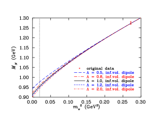
This $\chi$EFT extrapolation scheme to order $\mathcal{O}(m_{\pi}^{4}\,\mathrm{log}\,m_{\pi})$ will be used in conjunction with lattice QCD data from JLQCD, PACS-CS and CP-PACS to predict the nucleon mass for any value of $m_{\pi}^{2}$. The lattice data used in this analysis can be used to extrapolate $M_{N}$ to the physical point by taking into account the relevant curvature from the loop integrals in Eqs.  (18), (20) and (22). As an example, a regulator value of $\Lambda=1.0$ GeV was chosen for Figures 9 through 11, where the finite volume corrected EFT appears concordant with previous QCDSF-UKQCD results Ali Khan et al. (2004). If the regulator is changed away from the choice $\Lambda=1.0$ GeV, the extrapolation curve also changes. This signifies a scheme dependence in the result due to using lattice QCD data beyond the PCR.

To demonstrate this, consider the infinite volume extrapolation of the CP-PACS data. The extrapolation is achieved by subtracting the finite volume loop integral contributions defined in Eqs. (17), (19) and (21) from each data point and then fitting the result to obtain the coefficients $c_{0}$, $c_{2}$ and $a_{4}^{\Lambda}$ as shown in Eq. (27). The infinite volume loop integrals are then added back at any desired value of $m_{\pi}^{2}$.

Figure 11 shows that the curves overlap exactly when $m_{\pi}^{2}$ is large, where the lattice data reside. They diverge as the chiral regime is approached. This section addresses this problem in detail.

Figure 8: (color online). Example dipole extrapolation based on JLQCD data Ohki et al. (2008), box size: $1.9$ fm.

Figure 9: (color online). Example dipole extrapolation based on PACS-CS data Aoki et al. (2008), box size: $2.9$ fm.

Figure 10: (color online). Example dipole extrapolation based on CP-PACS data Ali Khan et al. (2002), box size: $2.3-2.8$ fm.

Figure 11: (color online). Close zoom of the regulator dependence for dipole extrapolation based on CP-PACS data. Only the data point corresponding to the smallest $m_{\pi}^{2}$ value is shown at this scale.

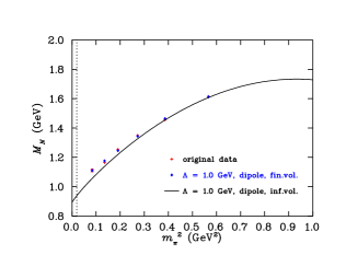
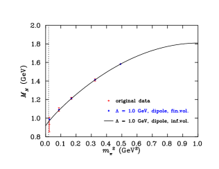
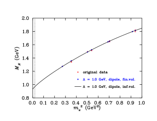
A particular regularization scale is selected and a dense and precise data set is generated, which smoothly connects with state of the art lattice simulation results. If all the data considered lie within the PCR then the choice of regulator parameter is irrelevant, and the FRR chiral expansion is mathematically equivalent to scale-invariant renormalzation schemes including DR. However, the purpose here is to consider an insightful scenario, whereby a set of ideal pseudodata with known low energy coefficients is produced. This scenario will form the basis of the investigation of the PCR, and ultimately the possible existence of an intrinsic scale hidden within the actual lattice QCD data.

The pseudodata are produced by performing a finite volume extrapolation such as shown in Figures 9 through 11. The difference is that $100$ infinite volume extrapolation points are produced close to the chiral regime. The exercise is to pretend that it is actual lattice QCD data. Clearly, a regularization scheme must be chosen to produce the pseudodata. In this case, a dipole regulator was chosen and pseudodata were created at $\Lambda_{\mathrm{c}}\equiv 1.0$ GeV.

The regularization dependence of the extrapolation is characterized by the scale dependence of the renormalized constants $c_{i}$. Consider how $c_{0}$ and $c_{2}$ behave when analyzed with a variety of regulator values in Figures 13 and 13. By choosing to use pseudodata produced at infinite volume, one eliminates the concern that behaviour of the low energy constants across a range of regulators and pion masses is a finite volume artefact. The equivalents of Figures 13 and 13 for finite volume pseudodata exhibit the same features.

Figure 12: (color online). Behaviour of $c_{0}$ vs. regulator parameter $\Lambda$, based on infinite volume pseudodata created with a dipole regulator at $\Lambda_{\mathrm{c}}=1.0$ GeV (based on lightest four data points from PACS-CS). Each curve uses pseudodata with a different upper value of pion mass $m_{\pi,\mathrm{max}}^{2}$.

Figure 13: (color online). Behaviour of $c_{2}$ vs. $\Lambda$, based on infinite volume pseudodata created with a dipole regulator at $\Lambda_{\mathrm{c}}=1.0$ GeV (based on lightest four data points from PACS-CS). Each curve uses pseudodata with a different upper value of pion mass $m_{\pi,\mathrm{max}}^{2}$.

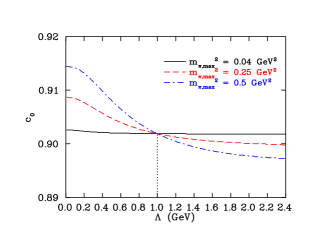
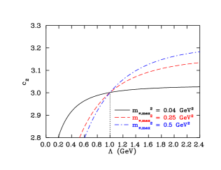
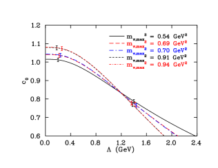
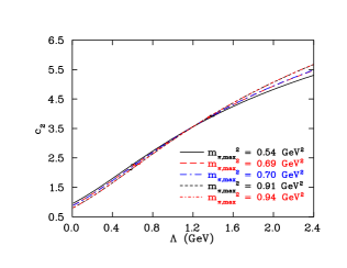
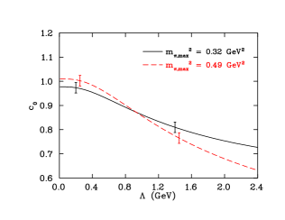
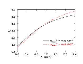
If three pseudodata sets are compared, each with different upper bounds on the range of $m_{\pi}^{2}$ considered in the fit, an increasing regulator dependence in $c_{0}$ and $c_{2}$ is seen further from the PCR. A steep line indicates a strong scheme dependence in the result, and naturally occurs for data samples extending far outside the PCR. Scheme independence will appear as a completely horizontal graph. The latter is what one expects for a value of $m_{\pi,\mathrm{max}}^{2}<0.04$ GeV², as shown in Figures 13 and 13. Note that, for each figure, all three curves (corresponding to different $m_{\pi,\mathrm{max}}^{2}$) arrive at stable values for $c_{0}$ and $c_{2}$ on the righthand side of the graph (large $\Lambda$). To read off the values of $c_{0}$ and $c_{2}$ for large $\Lambda$ is tempting but wrong. It is known that the correct values of $c_{0}$ and $c_{2}$ are recovered at $\Lambda=1.0$ GeV, because at that value the pseudodata were created.

The analysis of the pseudodata in Figures 13 and 13 shows that as the value of $m_{\pi,\mathrm{max}}^{2}$ is changed, the correct value of $c_{0}$ is recovered at exactly $\Lambda=\Lambda_{\mathrm{c}}$, where the curves intersect. This is also the intersection point for $c_{2}$ at $\Lambda=\Lambda_{\mathrm{c}}$. This suggests that when considering lattice QCD results extending outside the PCR, there may be an optimal finite-range cutoff. Physically, such a cutoff would be associated with an intrinsic scale reflecting the finite size of the source of the pion dressings. Mathematically, this optimal cutoff is reflected by an independence of the fit parameters on $m_{\pi,\mathrm{max}}^{2}$.

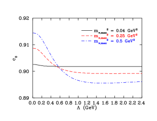
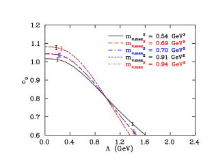
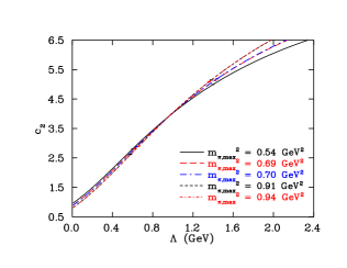
To illustrate the non-triviality of this scale of curve-intersection, the pseudodata were analyzed with a different regulator, e.g. a triple-dipole regulator. Figures 15 and 15 show that the scale of the intersection is no longer a clear point, but a cluster centred about $0.5$ to $0.6$ GeV. The triple-dipole will of course predict a different ‘best scale’, since the shape of the regulator is different from that of the dipole used to create the pseudodata. The essential point of this exercise is that clustering of curve intersections identifies a preferred renormalization scale that allows one to recover the correct low energy coefficients. In this case, the crossing of the dash and dot-dash curves (from fitting) clearly identifies $\Lambda^{\mathrm{scale}}_{\mathrm{trip}}=0.6$ GeV as a preferred regulator, which reflects the intrinsic scale used to create the data. Table 1 compares the values for $c_{0}$ and $c_{2}$ recovered in this analysis for two different regulators: the preferred value $\Lambda^{\mathrm{scale}}_{\mathrm{trip}}=0.6$ GeV, and a large value $\Lambda_{\mathrm{trip}}=2.4$ GeV reflecting the asymptotic result recovered from DR. The input values of $c_{0}$ and $c_{2}$ used to create the pseudodata are also indicated.

parameter	input	$\Lambda^{\mathrm{scale}}_{\mathrm{trip}}=0.6$	$\Lambda_{\mathrm{trip}}=2.4$	$\Lambda_{\mathrm{trip}}=2.4$
		$m_{\pi,\mathrm{max}}^{2}=0.25$	$m_{\pi,\mathrm{max}}^{2}=0.25$	$m_{\pi,\mathrm{max}}^{2}=0.5$
$c_{0}$	$0.902$	$0.901$	$0.899$	$0.896$
$c_{2}$	$3.00$	$3.07$	$3.17$	$3.23$

Table 1: A comparison of the parameters $c_{0}$ (GeV) and $c_{2}$ (GeV^-1) at their input value (pseudodata created with a dipole at $\Lambda_{\mathrm{c}}=1.0$ GeV) with the values when analysed with a triple dipole regulator. Different values of $\Lambda_{\mathrm{trip}}$ (GeV) and $m_{\pi,\mathrm{max}}^{2}$ (GeV²) are chosen to demonstrate the scheme dependence of $c_{0}$ and $c_{2}$ for data extending outside the PCR.

Figure 14: (color online). Behaviour of $c_{0}$ vs. $\Lambda$, based on infinite volume pseudodata created with a dipole regulator at $\Lambda_{\mathrm{c}}=1.0$ GeV but subsequently analyzed using a triple-dipole regulator.

Figure 15: (color online). Behaviour of $c_{2}$ vs. $\Lambda$, based on infinite volume pseudodata created with a dipole regulator at $\Lambda_{\mathrm{c}}=1.0$ GeV but subsequently analyzed using a triple-dipole regulator.

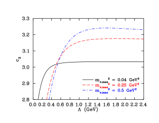
Note that the finite-range renormalization scheme breaks down if the finite-range regulator is too small. This is because $\Lambda$ must be large enough to include the chiral physics being studied. The exact value of a sensible lower bound in the finite-range regulator will depend on the functional form chosen as regulator. This is estimated for three dipole-like regulators in Section (IV).

Figure 13 shows that the renormalization for $c_{2}$ breaks down for small values of the regulator $\Lambda$. FRR breaks down for a value of $\Lambda_{\mathrm{dip}}$ much below $0.6$ GeV, because the coefficients $b_{i}$ of the loop integral expansion in Eqs. (18), (20) and (22) are proportional to $\Lambda^{(3-i)}$. For high-order terms with large $i$, the coefficients will become large when $\Lambda$ is small. This will adversely affect the convergence properties of the chiral expansion. One obtains a residual series expansion with good convergence properties only when $\Lambda$ reflects the intrinsic scale of the source of the pion dressings of the hadron in question.

The pseudodata analysis provides a good indication of a lower bound for $\Lambda$ using a dipole regulator: $\Lambda_{\mathrm{dip}}\gtrsim 0.6$ GeV. Similarly, Figure 15 suggests a lower bound for the triple dipole regulator: $\Lambda_{\mathrm{trip}}\gtrsim 0.3$ GeV. The same analysis can be repeated for the double dipole regulator to obtain $\Lambda_{\mathrm{doub}}\gtrsim 0.4$ GeV.

One may also constrain the lowest value that $\Lambda$ can take by considering phenomenological arguments. Based on the physical values of the sigma commutator and the nucleon mass, a pion mass of $m_{\pi}\approx 0.5$ GeV bounds the radius of convergence Borasoy et al. (2002); Young et al. (2009); Young and Thomas (2009). Therefore, in order to ensure the inclusion of important contributions to the chiral physics, one should choose an energy scale $\Lambda_{\mathrm{sharp}}\sim 0.5$ GeV for a sharp cutoff (step function) regulator. To compare this estimate for the sharp cutoff to that of dipole-like regulators, one can calculate the regulator value required such that $u^{2}_{n}(k^{2})=1/2$ when the momentum takes the energy scale of $\Lambda_{\mathrm{sharp}}$. This results in a rough estimate for a sensible value for the dipole, double dipole and triple dipole. These values are $\Lambda_{\mathrm{dip}}\sim 1.1$ GeV, $\Lambda_{\mathrm{doub}}\sim 0.76$ GeV and $\Lambda_{\mathrm{trip}}\sim 0.66$ GeV, respectively. In any event, a wide range of regulator values will be considered, and the intersections of the curves for the low energy coefficients will be used in order to construct fits outside the PCR. This will be done in order to identify the presence of an intrinsic scale for the pion source and an associated preferred regularization scale.

IV Intrinsic Scale: Lattice Results

IV.1 Evidence for an Intrinsic Scale

In the example of the pseudodata, an optimal finite-range cutoff was obtained from the data themselves. Clearly, the pseudodata have an intrinsic scale: the renormalization scale $\Lambda_{\mathrm{c}}$ at which they were created. This test example leads the researcher to wonder if actual lattice QCD data have an intrinsic cutoff scale embedded within them. That is, by analysing lattice QCD data in the same way as the pseudodata, can a similar intersection point be obtained from the renormalization scale flow of $c_{0}$ and $c_{2}$? If so, this indicates that the lattice QCD data contain information regarding an optimal finite-range regularization scale, which can be calculated.

The results for the renormalization of $c_{0}$ and $c_{2}$ as a function of $\Lambda$ are now presented for JLQCD Ohki et al. (2008), PACS-CS Aoki et al. (2008) and CP-PACS Ali Khan et al. (2002) lattice QCD data. The JLQCD data use overlap fermions in two-flavor QCD, but the lattice box size for each data point is $\sim 1.9$ fm, smaller than the other two data sets. The PACS-CS data use the nonperturbatively $\mathcal{O}(a)$-improved Wilson quark action at a lattice box size of $\sim 2.9$ fm, but the data set only contains five data points and a large statistical error in the smallest $m_{\pi}^{2}$ point. The CP-PACS data use a mean field improved clover quark action on lattice box sizes for each data point varying from $\sim 2.2$ fm to $\sim 2.8$ fm.

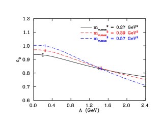
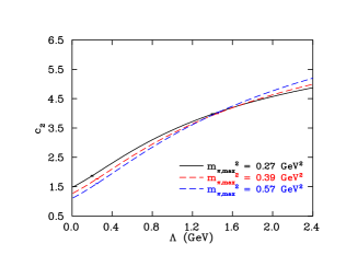
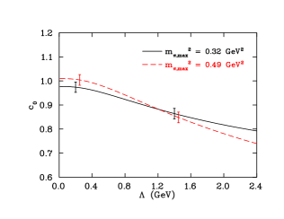
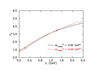
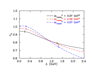
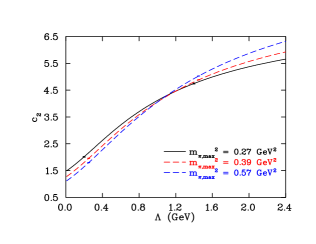
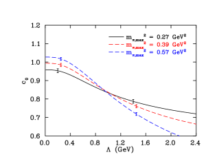
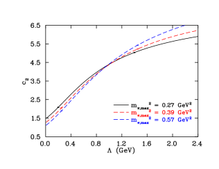
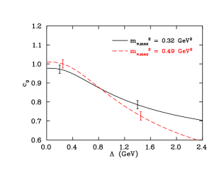
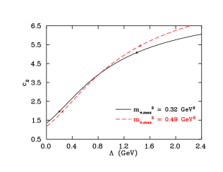
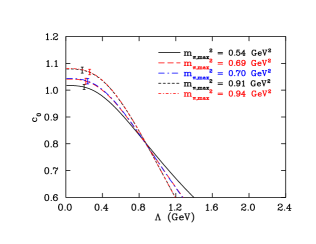
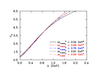
The chiral expansion is first used to chiral order $\mathcal{O}(m_{\pi}^{3})$. In this case, the fit parameters are $c_{0}$ and $c_{2}$ only. The results for a dipole regulator are shown in Figures 19 through 21, the results for the double dipole case are shown in Figures 25 through 27 and the results for the triple dipole are shown in Figures 31 through 33. To estimate the statistical error in the renormalized constants $\delta c$, a bootstrap technique of $200$ configurations of nucleon mass data is used. The configurations differ by the statistical error in the data, with values generated by a Gaussian distribution. In each plot, the same configurations are used for a variety of values of $\Lambda$ considered. A few points are selected in Figures 19 through 33 to indicate the general size of the statistical error bars.

It should be noted that none of these curves is flat to within $1\%$ accuracy. All fits have included data beyond the commonly accepted PCR. Clearly, there is a well-defined intersection point in the renormalization flow curves. Also, the value of $\Lambda$ at which the intersection point occurs is the same even for different data sets, and for different $c_{i}$. The tight groupings of the curve crossings lend credence to the ansatz of an intrinsic scale associated with the finite size of the source of the pion dressings of the nucleon. This is a central result of this analysis.

An intrinsic scale of $\Lambda^{\mathrm{scale}}_{\mathrm{dip}}\approx 1.3$ GeV was obtained for the dipole, $\Lambda^{\mathrm{scale}}_{\mathrm{doub}}\approx 1.0$ GeV for the double dipole and $\Lambda^{\mathrm{scale}}_{\mathrm{trip}}\approx 0.9$ GeV for the triple dipole. These values differ because the regulators have different shapes, and different values of $\Lambda^{\mathrm{scale}}$ are required to create a similar suppression of large loop momenta.

Figure 16: (color online). Behaviour of $c_{0}$ vs. $\Lambda$, based on JLQCD data. The chiral expansion is taken to order $\mathcal{O}(m_{\pi}^{3})$, and a dipole regulator is used. A few points are selected to indicate the general size of the statistical error bars.

Figure 17: (color online). Behaviour of $c_{2}$ vs. $\Lambda$, based on JLQCD data. The chiral expansion is taken to order $\mathcal{O}(m_{\pi}^{3})$, and a dipole regulator is used. A few points are selected to indicate the general size of the statistical error bars.

Figure 18: (color online). Behaviour of $c_{0}$ vs. $\Lambda$, based on PACS-CS data. The chiral expansion is taken to order $\mathcal{O}(m_{\pi}^{3})$, and a dipole regulator is used. A few points are selected to indicate the general size of the statistical error bars.

Figure 19: (color online). Behaviour of $c_{2}$ vs. $\Lambda$, based on PACS-CS data. The chiral expansion is taken to order $\mathcal{O}(m_{\pi}^{3})$, and a dipole regulator is used. A few points are selected to indicate the general size of the statistical error bars.

Figure 20: (color online). Behaviour of $c_{0}$ vs. $\Lambda$, based on CP-PACS data. The chiral expansion is taken to order $\mathcal{O}(m_{\pi}^{3})$, and a dipole regulator is used. A few points are selected to indicate the general size of the statistical error bars.

Figure 21: (color online). Behaviour of $c_{2}$ vs. $\Lambda$, based on CP-PACS data. The chiral expansion is taken to order $\mathcal{O}(m_{\pi}^{3})$, and a dipole regulator is used. A few points are selected to indicate the general size of the statistical error bars.

Figure 22: (color online). Behaviour of $c_{0}$ vs. $\Lambda$, based on JLQCD data. The chiral expansion is taken to order $\mathcal{O}(m_{\pi}^{3})$ and a double dipole regulator is used. A few points are selected to indicate the general size of the statistical error bars.

Figure 23: (color online). Behaviour of $c_{2}$ vs. $\Lambda$, based on JLQCD data. The chiral expansion is taken to order $\mathcal{O}(m_{\pi}^{3})$ and a double dipole regulator is used. A few points are selected to indicate the general size of the statistical error bars.

Figure 24: (color online). Behaviour of $c_{0}$ vs. $\Lambda$, based on PACS-CS data. The chiral expansion is taken to order $\mathcal{O}(m_{\pi}^{3})$ and a double dipole regulator is used. A few points are selected to indicate the general size of the statistical error bars.

Figure 25: (color online). Behaviour of $c_{2}$ vs. $\Lambda$, based on PACS-CS data. The chiral expansion is taken to order $\mathcal{O}(m_{\pi}^{3})$ and a double dipole regulator is used. A few points are selected to indicate the general size of the statistical error bars.

Figure 26: (color online). Behaviour of $c_{0}$ vs. $\Lambda$, based on CP-PACS data. The chiral expansion is taken to order $\mathcal{O}(m_{\pi}^{3})$ and a double dipole regulator is used. A few points are selected to indicate the general size of the statistical error bars.

Figure 27: (color online). Behaviour of $c_{2}$ vs. $\Lambda$, based on CP-PACS data. The chiral expansion is taken to order $\mathcal{O}(m_{\pi}^{3})$ and a double dipole regulator is used. A few points are selected to indicate the general size of the statistical error bars.

Figure 28: (color online). Behaviour of $c_{0}$ vs. $\Lambda$, based on JLQCD data. The chiral expansion is taken to order $\mathcal{O}(m_{\pi}^{3})$ and a triple dipole regulator is used. A few points are selected to indicate the general size of the statistical error bars.

Figure 29: (color online). Behaviour of $c_{2}$ vs. $\Lambda$, based on JLQCD data. The chiral expansion is taken to order $\mathcal{O}(m_{\pi}^{3})$ and a triple dipole regulator is used. A few points are selected to indicate the general size of the statistical error bars.

Figure 30: (color online). Behaviour of $c_{0}$ vs. $\Lambda$, based on PACS-CS data. The chiral expansion is taken to order $\mathcal{O}(m_{\pi}^{3})$ and a triple dipole regulator is used. A few points are selected to indicate the general size of the statistical error bars.

Figure 31: (color online). Behaviour of $c_{2}$ vs. $\Lambda$, based on PACS-CS data. The chiral expansion is taken to order $\mathcal{O}(m_{\pi}^{3})$ and a triple dipole regulator is used. A few points are selected to indicate the general size of the statistical error bars.

Figure 32: (color online). Behaviour of $c_{0}$ vs. $\Lambda$, based on CP-PACS data. The chiral expansion is taken to order $\mathcal{O}(m_{\pi}^{3})$ and a triple dipole regulator is used. A few points are selected to indicate the general size of the statistical error bars.

Figure 33: (color online). Behaviour of $c_{2}$ vs. $\Lambda$, based on CP-PACS data. The chiral expansion is taken to order $\mathcal{O}(m_{\pi}^{3})$ and a triple dipole regulator is used. A few points are selected to indicate the general size of the statistical error bars.

IV.2 Statistical Errors

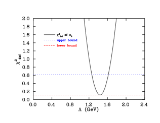
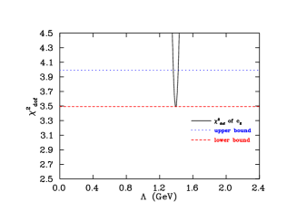
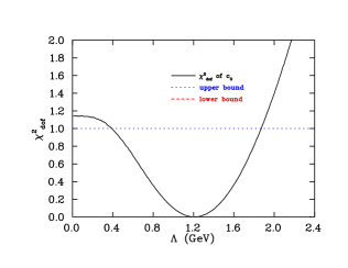
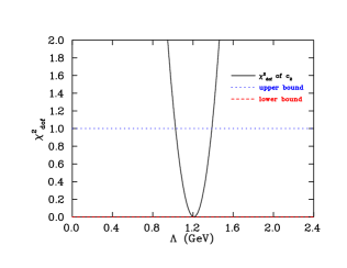
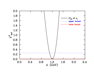
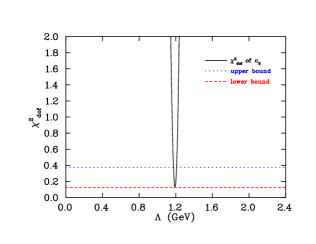
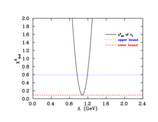
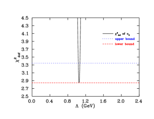
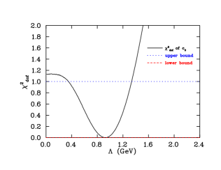
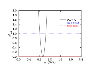
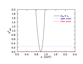
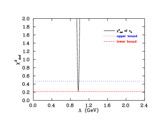
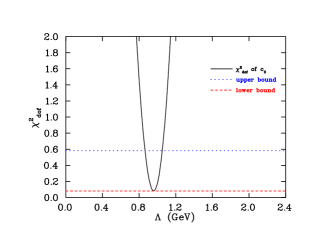
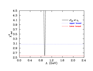
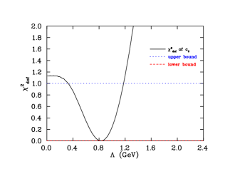
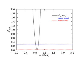
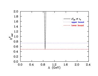
On each renormalization plot in Figures 19 through 33 there are many curves, each corresponding to different values of $m_{\pi,\mathrm{max}}^{2}$. It is of primary interest to what extent these curves match. Therefore, a $\chi^{2}_{dof}$ should be constructed, where $dof$ equals the number of curves on each plot minus one for the best fit value of $c_{0}$ or $c_{2}$, denoted by $c^{T}$ in the following. This also serves to quantify the constraint on the intrinsic scale $\Lambda^{\mathrm{scale}}$. The $\chi^{2}_{dof}$ is evaluated separately for each renormalized constant $c$ (with error $\delta c$) and regulator value $\Lambda$:

$$\chi^{2}_{dof}=\frac{1}{n-1}\sum_{i=1}^{n}\frac{{(c_{i}(\Lambda)-c^{T}(\Lambda))}^{2}}{{(\delta c_{i}(\Lambda))}^{2}}\,,$$ (31)

for $i$ corresponding to data sets with differing $m_{\pi,\mathrm{max}}^{2}$. The theoretical value $c^{T}$ is given by the weighted mean:

$$c^{T}(\Lambda)=\frac{\sum_{i=1}^{n}c_{i}(\Lambda)/{{(\delta c_{i}(\Lambda))}^{2}}}{\sum_{j=1}^{n}1/{(\delta c_{j}(\Lambda))}^{2}}\,.$$ (32)

The $\chi^{2}_{dof}$ can be calculated as a function of the regulator parameter $\Lambda$ for each of the renormalization plots of Figures 19 through 33. In the case of the PACS-CS data, the minimum of the $\chi^{2}_{dof}$ curve will be centred at the intersection point. In the case of the JLQCD and CP-PACS data, there appears to be a single intersection point on each plot, but in fact there are multiple intersections over a very small window of $\Lambda$. The results for $\chi^{2}_{dof}$ will indicate the ‘best’ central value of $\Lambda$. This central value of $\Lambda$ will be taken to be the intrinsic scale. The $\chi^{2}_{dof}$ curves for a dipole regulator are shown in Figures 37 through 39, the $\chi^{2}_{dof}$ curves for the double dipole case are shown in Figures 43 through 45 and the $\chi^{2}_{dof}$ curves for the triple dipole are shown in Figures 49 through 51.

Figure 34: (color online). Behaviour of $\chi^{2}_{dof}$ for $c_{0}$ vs. $\Lambda$, based on JLQCD data. The chiral expansion is taken to order $\mathcal{O}(m_{\pi}^{3})$, and a dipole regulator is used.

Figure 35: (color online). Behaviour of $\chi^{2}_{dof}$ for $c_{2}$ vs. $\Lambda$, based on JLQCD data. The chiral expansion is taken to order $\mathcal{O}(m_{\pi}^{3})$, and a dipole regulator is used.

Figure 36: (color online). Behaviour of $\chi^{2}_{dof}$ for $c_{0}$ vs. $\Lambda$, based on PACS-CS data. The chiral expansion is taken to order $\mathcal{O}(m_{\pi}^{3})$, and a dipole regulator is used.

Figure 37: (color online). Behaviour of $\chi^{2}_{dof}$ for $c_{2}$ vs. $\Lambda$, based on PACS-CS data. The chiral expansion is taken to order $\mathcal{O}(m_{\pi}^{3})$, and a dipole regulator is used.

Figure 38: (color online). Behaviour of $\chi^{2}_{dof}$ for $c_{0}$ vs. $\Lambda$, based on CP-PACS data. The chiral expansion is taken to order $\mathcal{O}(m_{\pi}^{3})$, and a dipole regulator is used.

Figure 39: (color online). Behaviour of $\chi^{2}_{dof}$ for $c_{2}$ vs. $\Lambda$, based on CP-PACS data. The chiral expansion is taken to order $\mathcal{O}(m_{\pi}^{3})$, and a dipole regulator is used.

Figure 40: (color online). Behaviour of $\chi^{2}_{dof}$ for $c_{0}$ vs. $\Lambda$, based on JLQCD data. The chiral expansion is taken to order $\mathcal{O}(m_{\pi}^{3})$, and a double dipole regulator is used.

Figure 41: (color online). Behaviour of $\chi^{2}_{dof}$ for $c_{2}$ vs. $\Lambda$, based on JLQCD data. The chiral expansion is taken to order $\mathcal{O}(m_{\pi}^{3})$, and a double dipole regulator is used.

Figure 42: (color online). Behaviour of $\chi^{2}_{dof}$ for $c_{0}$ vs. $\Lambda$, based on PACS-CS data. The chiral expansion is taken to order $\mathcal{O}(m_{\pi}^{3})$, and a double dipole regulator is used.

Figure 43: (color online). Behaviour of $\chi^{2}_{dof}$ for $c_{2}$ vs. $\Lambda$, based on PACS-CS data. The chiral expansion is taken to order $\mathcal{O}(m_{\pi}^{3})$, and a double dipole regulator is used.

Figure 44: (color online). Behaviour of $\chi^{2}_{dof}$ for $c_{0}$ vs. $\Lambda$, based on CP-PACS data. The chiral expansion is taken to order $\mathcal{O}(m_{\pi}^{3})$, and a double dipole regulator is used.

Figure 45: (color online). Behaviour of $\chi^{2}_{dof}$ for $c_{2}$ vs. $\Lambda$, based on CP-PACS data. The chiral expansion is taken to order $\mathcal{O}(m_{\pi}^{3})$, and a double dipole regulator is used.

Figure 46: (color online). Behaviour of $\chi^{2}_{dof}$ for $c_{0}$ vs. $\Lambda$, based on JLQCD data. The chiral expansion is taken to order $\mathcal{O}(m_{\pi}^{3})$, and a triple dipole regulator is used.

Figure 47: (color online). Behaviour of $\chi^{2}_{dof}$ for $c_{2}$ vs. $\Lambda$, based on JLQCD data. The chiral expansion is taken to order $\mathcal{O}(m_{\pi}^{3})$, and a triple dipole regulator is used.

Figure 48: (color online). Behaviour of $\chi^{2}_{dof}$ for $c_{0}$ vs. $\Lambda$, based on PACS-CS data. The chiral expansion is taken to order $\mathcal{O}(m_{\pi}^{3})$, and a triple dipole regulator is used.

Figure 49: (color online). Behaviour of $\chi^{2}_{dof}$ for $c_{2}$ vs. $\Lambda$, based on PACS-CS data. The chiral expansion is taken to order $\mathcal{O}(m_{\pi}^{3})$, and a triple dipole regulator is used.

Figure 50: (color online). Behaviour of $\chi^{2}_{dof}$ for $c_{0}$ vs. $\Lambda$, based on CP-PACS data. The chiral expansion is taken to order $\mathcal{O}(m_{\pi}^{3})$, and a triple dipole regulator is used.

Figure 51: (color online). Behaviour of $\chi^{2}_{dof}$ for $c_{2}$ vs. $\Lambda$, based on CP-PACS data. The chiral expansion is taken to order $\mathcal{O}(m_{\pi}^{3})$, and a triple dipole regulator is used.

IV.3 Higher Chiral Order

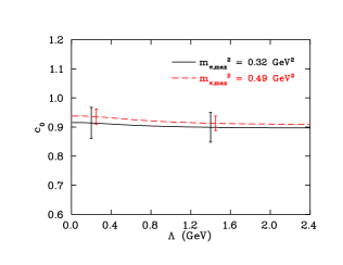
Consider the renormalization of $c_{0}$ and $c_{2}$ as a function of $\Lambda$, for chiral order $\mathcal{O}(m_{\pi}^{4}\,\mathrm{log}\,m_{\pi})$. The results for PACS-CS and CP-PACS data are shown in Figures 55 through 55, as an example. In this case, no clear intersection points in the renormalization curves can be found, and so one is unable to specify an intrinsic scale. This certainly should be the case when working with data entirely within the PCR, because all renormalization procedures would be equivalent (to a prescribed level of accuracy) and so there would be no optimal regulator parameter. It is known that this is not the case for the data sets used in this study. This is verified by considering the evident scale dependence of $c_{0}$ and $c_{2}$ in Figures 55 through 55. The fact that $c_{0}$ and $c_{2}$ change over the range of $\Lambda$ values indicates that the data are not inside the PCR. Further, since no preferred scale is revealed, any choice of $\Lambda$ appears equivalent at this order. While this is encouraging that the scheme dependence is being weakened by working to higher order, it must be recognized that there is a systematic error associated with the choice of $\Lambda$. In the case of the CP-PACS results shown in Figures 55 and 55, it can be seen that the statistical errors are substantially smaller than the systematic error associated with a characteristic range, $\Lambda_{\mathrm{lower}}<\Lambda<\infty$, where $\Lambda_{\mathrm{lower}}$ is the lowest reasonable value of $\Lambda$.

Figure 52: (color online). Behaviour of $c_{0}$ vs. $\Lambda$, based on PACS-CS data. The chiral expansion taken to order $\mathcal{O}(m_{\pi}^{4}\,\mathrm{log}\,m_{\pi})$ and a dipole regulator is used. A few points are selected to indicate the general size of the statistical error bars.

Figure 53: (color online). Behaviour of $c_{2}$ vs. $\Lambda$, based on PACS-CS data. The chiral expansion taken to order $\mathcal{O}(m_{\pi}^{4}\,\mathrm{log}\,m_{\pi})$ and a dipole regulator is used. A few points are selected to indicate the general size of the statistical error bars.

Figure 54: (color online). Behaviour of $c_{0}$ vs. $\Lambda$, based on CP-PACS data. The chiral expansion taken to order $\mathcal{O}(m_{\pi}^{4}\,\mathrm{log}\,m_{\pi})$ and a dipole regulator is used. A few points are selected to indicate the general size of the statistical error bars.

Figure 55: (color online). Behaviour of $c_{2}$ vs. $\Lambda$, based on CP-PACS data. The chiral expansion taken to order $\mathcal{O}(m_{\pi}^{4}\,\mathrm{log}\,m_{\pi})$ and a dipole regulator is used. A few points are selected to indicate the general size of the statistical error bars.

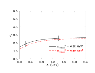
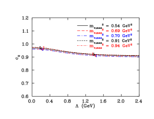
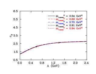
Since it is difficult to identify the intrinsic scale at this chiral order, the results for chiral order $\mathcal{O}(m_{\pi}^{3})$ will be chosen to demonstrate the process of handling the existence of an optimal regulator scale in lattice QCD data. The results for the calculation of the intrinsic scales $\Lambda^{\mathrm{scale}}$ for different data sets and regulators are given in Table 2. This table simply summarizes the central values from Figures 37 through 51. Such excellent agreement between the $c_{0}$ analysis and the $c_{2}$ analysis is remarkable, and indicative of the existence of an instrinsic scale in the data. There is also consistency among independent data sets. It is important to realize that the value of $\Lambda^{\mathrm{scale}}$ is always the order of $\sim 1$ GeV, not $10$ GeV, nor $100$ GeV; nor is it infinity.

	regulator form
optimal scale	dipole	double	triple
$\Lambda^{\mathrm{scale}}_{c_{0},\mathrm{JLQCD}}$	$1.44$	$1.08$	$0.96$
$\Lambda^{\mathrm{scale}}_{c_{2},\mathrm{JLQCD}}$	$1.40$	$1.05$	$0.94$
$\Lambda^{\mathrm{scale}}_{c_{0},\mathrm{PACS-CS}}$	$1.21$	$0.93$	$0.83$
$\Lambda^{\mathrm{scale}}_{c_{2},\mathrm{PACS-CS}}$	$1.21$	$0.93$	$0.83$
$\Lambda^{\mathrm{scale}}_{c_{0},\mathrm{CP-PACS}}$	$1.20$	$0.98$	$0.88$
$\Lambda^{\mathrm{scale}}_{c_{2},\mathrm{CP-PACS}}$	$1.19$	$0.97$	$0.87$

Table 2: Values of the central $\Lambda$ value in GeV, taken from the $\chi^{2}_{dof}$ analysis for $c_{0}$ and $c_{2}$, based on JLQCD, PACS-CS and CP-PACS data.

In calculating the systematic uncertainty in the observables $c_{0}$, $c_{2}$ and the nucleon mass at the physical point due to the intrinsic scale at order $\mathcal{O}(m_{\pi}^{4}\,\mathrm{log}\,m_{\pi})$, two methods are provided. Firstly, the upper and lower bounds from the $\chi^{2}_{dof}$ analysis at order $\mathcal{O}(m_{\pi}^{3})$ will be used to constrain $\Lambda$, and taken to be an accurate estimate of the systematic uncertainty in the contributions of higher order terms. Secondly, variation of the observables across the characteristic range of scale values, $\Lambda_{\mathrm{lower}}<\Lambda<\infty$ will be used, where $\Lambda_{\mathrm{lower}}$ takes the value of $0.6$, $0.4$ and $0.3$ GeV for the dipole, double dipole and triple dipole regulator, respectively. The results from both of these methods are displayed in Table 3.

The final results for the calculation of the renormalized constants $c_{0}$, $c_{2}$ and the nucleon mass extrapolated to the physical point ($m_{\pi,\mathrm{phys}}=140$ MeV) are summarized in Table 4. The lightest four data points from each of JLQCD, PACS-CS and CP-PACS lattice QCD data are used. The nucleon mass is calculated at the scale determined by the data.

	regulator form
sys. err.	dipole		double		triple
$\delta^{\Lambda}\!c_{0}^{\mathrm{JLQCD}}$	$0.001$,	$0.009$	$0.001$,	$0.013$	$0.001$,	$0.016$
$\delta^{\Lambda}\!c_{0}^{\mathrm{PACS-CS}}$	$0.005$,	$0.006$	$0.005$,	$0.010$	$0.006$,	$0.012$
$\delta^{\Lambda}\!c_{0}^{\mathrm{CP-PACS}}$	$0.002$,	$0.024$	$0.002$,	$0.037$	$0.002$,	$0.045$
$\delta^{\Lambda}\!c_{2}^{\mathrm{JLQCD}}$	$0.02$,	$0.31$	$0.03$,	$0.38$	$0.01$,	$0.48$
$\delta^{\Lambda}\!c_{2}^{\mathrm{PACS-CS}}$	$0.18$,	$0.25$	$0.16$,	$0.33$	$0.14$,	$0.43$
$\delta^{\Lambda}\!c_{2}^{\mathrm{CP-PACS}}$	$0.02$,	$0.40$	$0.02$,	$0.58$	$0.02$,	$0.73$
$\delta^{\Lambda}\!M_{N,\mathrm{phys}}^{\mathrm{JLQCD}}$	$0.0004$,	$0.0051$	$0.0003$,	$0.0073$	$0.0003$,	$0.0090$
$\delta^{\Lambda}\!M_{N,\mathrm{phys}}^{\mathrm{PACS-CS}}$	$0.0022$,	$0.0030$	$0.0025$,	$0.0046$	$0.0025$,	$0.0058$
$\delta^{\Lambda}\!M_{N,\mathrm{phys}}^{\mathrm{CP-PACS}}$	$0.0012$,	$0.0175$	$0.0013$,	$0.0270$	$0.0014$,	$0.0326$

Table 3: Results at $\mathcal{O}(m_{\pi}^{4}\,\mathrm{log}\,m_{\pi})$ for the systematic error due to the intrinsic scale, calculated using two methods, for the values of $c_{0}$ (GeV), $c_{2}$ (GeV^-1) and the nucleon mass $M_{N}$ (GeV) extrapolated to the physical point ($m_{\pi,\mathrm{phys}}=140$ MeV). The first number in each column is the systematic error due to the intrinsic scale using the upper and lower bound from the $\chi^{2}_{dof}$ analysis at order $\mathcal{O}(m_{\pi}^{3})$. The second number is the systematic error due to the instrinsic scale across the whole range of $\Lambda$ values from the lowest reasonable value ($\Lambda=\Lambda_{\mathrm{lower}}$) obtained from the pseudodata analysis, to the asymptotic value ($\Lambda=\infty$).

	regulator form
parameter	dipole	double	triple	WM(1)	WM(2)
$c_{0}^{\mathrm{JLQCD}}$	$0.873(18)(16)$	$0.875(17)(16)$	$0.891(17)(16)$	$0.880(29)$	$0.879(32)$
$c_{0}^{\mathrm{PACS-CS}}$	$0.900(51)(15)$	$0.899(51)(14)$	$0.898(51)(14)$	$0.899(53)$	$0.899(55)$
$c_{0}^{\mathrm{CP-PACS}}$	$0.924(3)(8)$	$0.914(3)(7)$	$0.918(3)(7)$	$0.918(13)$	$0.920(37)$
$c_{2}^{\mathrm{JLQCD}}$	$3.09(9)(11)$	$3.18(9)(12)$	$3.20(9)(11)$	$3.16(18)$	$3.14(43)$
$c_{2}^{\mathrm{PACS-CS}}$	$3.06(32)(15)$	$3.15(31)(14)$	$3.17(31)(14)$	$3.13(39)$	$3.12(49)$
$c_{2}^{\mathrm{CP-PACS}}$	$2.54(5)(4)$	$2.70(5)(2)$	$2.71(5)(3)$	$2.66(18)$	$2.61(60)$
$M_{N,\mathrm{phys}}^{\mathrm{JLQCD}}$	$1.02(2)(9)$	$1.02(2)(9)$	$1.02(2)(9)$	$1.02(9)$	$1.02(9)$
$M_{N,\mathrm{phys}}^{\mathrm{PACS-CS}}$	$0.967(45)(43)$	$0.966(45)(43)$	$0.966(45)(43)$	$0.966(62)$	$0.966(62)$
$M_{N,\mathrm{phys}}^{\mathrm{CP-PACS}}$	$0.982(2)(40)$	$0.975(2)(43)$	$0.978(2)(42)$	$0.979(43)$	$0.979(50)$

Table 4: Results at $\mathcal{O}(m_{\pi}^{4}\,\mathrm{log}\,m_{\pi})$ for the values of $c_{0}$ (GeV), $c_{2}$ (GeV^-1) and the nucleon mass $M_{N}$ (GeV) extrapolated to the physical point ($m_{\pi,\mathrm{phys}}=140$ MeV). WM is the weighted mean of each row. The nucleon mass is calculated at the optimal scale $\Lambda^{\mathrm{scale}}$, which is the average of $\Lambda^{\mathrm{scale}}_{c_{0}}$ and $\Lambda^{\mathrm{scale}}_{c_{2}}$ for each data set. The extrapolations are performed at box sizes relevant to each data set: $L_{\mathrm{extrap}}^{\mathrm{JLQCD}}=1.9$ fm, $L_{\mathrm{extrap}}^{\mathrm{PACS-CS}}=2.9$ fm and $L_{\mathrm{extrap}}^{\mathrm{CP-PACS}}=2.8$ fm. The errors are quoted as the estimate of the statistical error first (based on random bootstrap configurations), and the systematic error obtained from the number of $m_{\pi}^{2}$ values used second. Two seperate weighted means are calculated for each row. WM(1) incorporates the systematic error in the intrinsic scale using the upper and lower bound from the $\chi^{2}_{dof}$ analysis at order $\mathcal{O}(m_{\pi}^{3})$. The WM(2) incorporates the systematic error due to the intrinsic scale across the whole range of $\Lambda$ values from the lowest reasonable value ($\Lambda=\Lambda_{\mathrm{lower}}$) obtained from the pseudodata analysis, to the asymptotic value ($\Lambda=\infty$). The weighted means also include an estimate of the systematic error in the choice of regulator. All errors are added in quadrature. Note that any order $\mathcal{O}(a)$ errors have not been incorporated into the total error analysis.

V Conclusion

In conclusion, it has been demonstrated that chiral effective field theory is an important tool for investigating the chiral properties of hadrons, and for extrapolating lattice QCD results. Because the chiral expansion is only convergent within a PCR, a renormalization scheme such as finite-range regularization should be used for current lattice QCD results, and into the foreseeable future. Renormalization scheme dependence occurs when lattice QCD data extending outside the PCR are used in the extrapolation. This provides a new quantitative test for determining when lattice QCD data lie within the PCR. As most lattice data extend beyond the PCR, a formalism was developed to determine if there is an optimal regularization scale $\Lambda^{\mathrm{scale}}$ in the finite-range regulator, and to calculate it if it exists. It was concluded that such an optimal scale can be obtained from the data itself by analyzing the renormalization flow curves of the low energy coefficients in the chiral expansion. The optimal scale is selected by the value for which the renormalized constants are independent of the upper bound of the fit domain. This also means that the renormalized constants are not to be identified with their asymptotic values at large $\Lambda$.

It was revealed that a preferred regularization scheme exists only for data sets extending outside the PCR. Such a preferred regularization scheme is associated with an intrinsic scale for the size of the pion dressings of the nucleon. By working to sufficiently high chiral order, it was discovered that the scale dependence was weakened. Nevertheless, the residual scale dependence persists as a significant component of the systematic uncertainty. For efficient propagation of this uncertainty, an interesting future direction would be to consider marginalization over the scale dependence Schindler and Phillips (2009). The described procedure was used to calculate the nucleon mass at the physical point, the low energy coefficients $c_{0}$ and $c_{2}$ and their associated statistical and systematic errors. Several different functional forms of regulator were considered, and lattice QCD data from JLQCD, PACS-CS and CP-PACS were used. An optimal cutoff scale $\Lambda^{\mathrm{scale}}$ for each set of lattice QCD data was obtained, and the systematic error in the choice of renormalization scheme was calculated.

In summary, the existence of a well defined intrinsic scale has been discovered. It has also been illustrated how its value can be determined from lattice QCD results.

References

- McGovern and Birse (1999) J. A. McGovern and M. C. Birse, Phys. Lett. B446, 300 (1999), eprint hep-ph/9807384.
- McGovern and Birse (2006) J. A. McGovern and M. C. Birse, Phys. Rev. D74, 097501 (2006), eprint hep-lat/0608002.
- Schindler et al. (2007) M. R. Schindler, D. Djukanovic, J. Gegelia, and S. Scherer, Phys. Lett. B649, 390 (2007), eprint hep-ph/0612164.
- Beane (2004a) S. R. Beane, Nucl. Phys. B695, 192 (2004a), eprint hep-lat/0403030.
- Leinweber et al. (2005a) D. B. Leinweber, A. W. Thomas, and R. D. Young, Nucl. Phys. A755, 59 (2005a), eprint hep-lat/0501028.
- Gell-Mann et al. (1968) M. Gell-Mann, R. J. Oakes, and B. Renner, Phys. Rev. 175, 2195 (1968).
- Leinweber et al. (2000) D. B. Leinweber, A. W. Thomas, and S. V. Wright, Phys. Lett. B482, 109 (2000), eprint hep-lat/0001007.
- Wright et al. (2000) S. V. Wright, D. B. Leinweber, and A. W. Thomas, Nucl. Phys. A680, 137 (2000), eprint nucl-th/0005003.
- Holl et al. (2006) A. Holl, P. Maris, C. D. Roberts, and S. V. Wright, Nucl. Phys. Proc. Suppl. 161, 87 (2006), eprint nucl-th/0512048.
- Donoghue et al. (1999) J. F. Donoghue, B. R. Holstein, and B. Borasoy, Phys. Rev. D59, 036002 (1999), eprint hep-ph/9804281.
- Young et al. (2002) R. D. Young, D. B. Leinweber, A. W. Thomas, and S. V. Wright, Phys. Rev. D66, 094507 (2002), eprint hep-lat/0205017.
- Young et al. (2003) R. D. Young, D. B. Leinweber, and A. W. Thomas, Prog. Part. Nucl. Phys. 50, 399 (2003), eprint hep-lat/0212031.
- Borasoy et al. (2002) B. Borasoy, B. R. Holstein, R. Lewis, and P. P. A. Ouimet, Phys. Rev. D66, 094020 (2002), eprint hep-ph/0210092.
- Leinweber et al. (2004) D. B. Leinweber, A. W. Thomas, and R. D. Young, Phys. Rev. Lett. 92, 242002 (2004), eprint hep-lat/0302020.
- Bernard et al. (2004) V. Bernard, T. R. Hemmert, and U.-G. Meissner, Nucl. Phys. A732, 149 (2004), eprint hep-ph/0307115.
- Djukanovic et al. (2005) D. Djukanovic, M. R. Schindler, J. Gegelia, and S. Scherer, Phys. Rev. D72, 045002 (2005), eprint hep-ph/0407170.
- Young et al. (2005) R. D. Young, D. B. Leinweber, and A. W. Thomas, Phys. Rev. D71, 014001 (2005), eprint hep-lat/0406001.
- Leinweber et al. (2005b) D. B. Leinweber et al., Phys. Rev. Lett. 94, 212001 (2005b), eprint hep-lat/0406002.
- Jenkins (1992) E. E. Jenkins, Nucl. Phys. B368, 190 (1992).
- Lebed (1995) R. F. Lebed, Phys. Rev. D51, 5039 (1995), eprint hep-ph/9411204.
- Beane (2004b) S. R. Beane, Phys. Rev. D70, 034507 (2004b), eprint hep-lat/0403015.
- Armour et al. (2006) W. Armour, C. R. Allton, D. B. Leinweber, A. W. Thomas, and R. D. Young, J. Phys. G32, 971 (2006), eprint hep-lat/0510078.
- Aoki et al. (2008) S. Aoki et al. (PACS-CS) (2008), eprint 0807.1661.
- Ali Khan et al. (2004) A. Ali Khan et al. (QCDSF-UKQCD), Nucl. Phys. B689, 175 (2004), eprint hep-lat/0312030.
- Ohki et al. (2008) H. Ohki et al., Phys. Rev. D78, 054502 (2008), eprint 0806.4744.
- Ali Khan et al. (2002) A. Ali Khan et al. (CP-PACS), Phys. Rev. D65, 054505 (2002), eprint hep-lat/0105015.
- Young et al. (2009) R. D. Young, J. M. M. Hall, and D. B. Leinweber (2009), eprint 0907.0408.
- Young and Thomas (2009) R. D. Young and A. W. Thomas (2009), eprint 0901.3310.
- Schindler and Phillips (2009) M. R. Schindler and D. R. Phillips, Annals Phys. 324, 682 (2009), eprint 0808.3643.