Entropy production and coarse-graining in Markov processes

Abstract

We study the large time fluctuations of entropy production in Markov processes. In particular, we consider the effect of a coarse-graining procedure which decimates fast states with respect to a given time threshold. Our results provide strong evidence that entropy production is not directly affected by this decimation, provided that it does not entirely remove loops carrying a net probability current. After the study of some examples of random walks on simple graphs, we apply our analysis to a network model for the kinesin cycle, which is an important biomolecular motor. A tentative general theory of these facts, based on Schnakenberg’s network theory, is proposed.

To our friend and colleague Massimo Falcioni, on his 60th birthday

I Introduction

The coarse-graining procedure is a fundamental ingredient of the statistical description of physical systems Ma (1985); Kadanoff (2000); Castiglione et al. (2008). By coarse-graining we mean a procedure which reduces the number of observables to simplify the physical description. For instance, it is used to describe the behaviour of the physically relevant quantities, or slow variables, which depends on the coupling among all variables characterizing the system of interest, including the so-called fast variables. The archetype of such a procedure is the treatment of Brownian colloidal particles, immersed in a fluid, in terms of the Langevin equation. In this sense any model meant to represent a real phenomenon may be thought of as a coarse-grained, i.e. reduced, description. The purpose of a model is, indeed, to advance our understanding of the object under investigation, by highlighting its interesting features and discarding the irrelevant ones. In turn, the roles of relevant and irrelevant characteristics depend on the purpose of the analysis to be performed. Furthermore, it isn’t always obvious which quantities should be listed as interesting, and which ones should be neglected, especially if a new problem is to be tackled Ma (1985); Kadanoff (2000); Castiglione et al. (2008); Bonaldi et al. (2009); Gregorio et al. (2009). Therefore, it is critical to understand how specific physical observables depend on the coarse-graining procedure.

Examples of coarse-grained descriptions at different resolution levels include the steps meant to connect the microscopic descriptions of systems of physical interest to the macroscopic ones, for instance the passage from the deterministic $\Gamma$-space description (positions and momenta of the $N$ particles) to the stochastic $\mu$-space description (position and momentum of one particle), up to macroscopic descriptions such as hydrodynamics, Fourier law, Navier-Stokes equations, etc.

Other methods use the coarse-graining procedure in order to reduce the number of variables, e.g. by a decimation method which suppresses the fast variables, or perform a spatial coarse-graining, as in the renormalization group approach. In these methods the coarse-graining is parametrized by some threshold, here denoted as coarse-graining level (CGL). This paper is devoted to the investigation of the impact of variations of CGL on the entropy production of non-equilibrium systems.

In the last decades, the introduction of the so-called Fluctuation Relations (FR) for deterministic dynamics, by Evans, Cohen, Morriss, Gallavotti, Jarzynski and other authors brought about important developements in the physics of far from equilibrium systems Evans et al. (1993); Gallavotti and Cohen (1995); Jarzynski (1997). In the specific context of Markov processes, here discussed, Lebowitz and Spohn Lebowitz and Spohn (1999) showed that the “entropy production” per unit time, measured on a time-interval $t$, $\mathcal{W}_{t}$ say, is described by a large deviation theory whose Cramer function, $C$, enjoys the following symmetry property:

$$C(\mathcal{W}_{t})-C(-\mathcal{W}_{t})=-\mathcal{W}_{t}~{}.$$

This relation is the stochastic counterpart of the deterministic steady state FR, and we call it Lebowitz-Spohn FR, or simply FR.

We remark that the FR does not provide any specific information about the shape of $C$. Therefore, a coarse-graining procedure which preserves the Markovian character of the model should preserve the validity of the FR as well, although it may change the shape of the Cramer function. As a matter of fact, Rahav and Jarzynski Rahav and Jarzynski (2007) argue that the validity of the FR is little affected by the coarse-graining procedure, even in nontrivial cases, such as those in which the decimation (or blocking) of variables results in the loss of the Markovian property.

In the present paper, at variance with Ref.Rahav and Jarzynski (2007), we do not address the question of validity of the FR (which is always satisfied by our models), but focus our attention on the effects of the decimation procedures on the behaviour of the Cramer function.

Understanding how $C$ changes under variations of the CGL is relevant, e.g. to interpret experimental results, since they are always obtained at finite resolution (for instance in frequency, Bonaldi et al. (2009)). Likewise, any model describing a real system is necessarily affected by some degree of approximation or of idealism. For instance, the entropy production defined by Lebowitz and Spohn appears to be a rather abstract quantity, depending on the direct and inverse trajectories in the state space, as well as on their probabilities in the stationary state, cf. Section II. Furthermore, such a quantity cannot be measured in a direct way. Therefore, it needs to be connected to directly measurable quantities, for its properties to be assessed.

Naively, one may expect the entropy production computed through a model which encompasses lots of details of the system of interest to be higher than that computed through less detailed models. Consider for example the Markov chain depicted in Fig. 1a, with transition probabilities $2\to 1$ and $3\to 4$ much larger than the remaining ones. One may impose that a net current flows from $3$ to $1$ and from $2$ to $4$, by choosing transition probabilities $P_{3\to 1}\ll P_{1\to 3}$ and $P_{2\to 4}\ll P_{4\to 2}$ and by tuning the other parameters so that all states have the same stationary probability.

Figure 1: A simple example of decimation which results in vanishing entropy production.

In this system, detailed balance does not hold, hence the mean entropy production is positive. However, the mean entropy production vanishes if the fast states $2$ and $3$ are decimated, and the Markov chain is reduced to the one represented in Fig. 1b, where $A$ corresponds to the old state $1$ and $B$ to the old state $4$. Indeed, detailed balance, which implies a vanishing entropy production, holds in any Markov chain with two states.

In the following we consider Markovian systems described by a Master equation:

$$\frac{dP_{n}}{dt}=\sum_{l\neq n}P_{l}W_{l\to n}-W_{n}^{0}P_{n}$$ (1)

where $W_{l\to n}$ is the transition rate from state $l$ to state $n$, with $l,n\in[1,N]$, $N$ being the number of possible states of the process, $P_{n}(t)$ is the probability to stay in the state $n$ at time $t$, and

$$W_{n}^{0}=\sum_{l\neq n}W_{n\to l}.$$ (2)

We adopt the coarse graining procedure introduced in Ref.Pigolotti and Vulpiani (2008) and described in Appendix A, which amounts to a decimation of all states whose characteristic times $\tau_{n}=1/W_{n}^{0}$ are smaller than a given $\Delta\tau>0$. The resulting master equation for the surviving states may be written as

$$\frac{d\tilde{P}_{j}}{dt}=\sum_{i\neq j}\tilde{P}_{i}\tilde{W}_{i\to j}-\tilde{W}_{j}^{0}\tilde{P}_{j}$$ (3)

with transition rates $\tilde{W}_{i\to j}$ as prescribed by Pigolotti and Vulpiani (2008), $i,j\in[1,\tilde{N}]$, $\tilde{N}<N$, and $\tilde{W}_{j}^{0}<1/\Delta\tau$ for all $j\in[1,\tilde{N}]$.

Varying $\Delta\tau$ the number of the slow states and the shape of the Cramer function $C_{\Delta\tau}(\mathcal{W}_{t})$ may in principle change.

In Section II, we present some numerical results for differently decimated Markov processes. In section III, we discuss the possibility of constructing a general theory, not yet available, of the decimation effects. In Section IV, we draw some conclusions and discuss open problems. Appendix A illustrates the decimation procedure; Appendix B reports analytical results about the effect of decimation on the current in a single loop; Appendix C recalls the graph analysis of currents in a Markov system, based on Schnakenberg’s theory; Appendix D describes in detail the kinesine model mentioned at the end of section II; Appendix E lists the main symbols used in the text.

II Some numerical results

II.1 Entropy production on a trajectory

While the concept of entropy production, or energy dissipation, dates a long time back de Groot and Mazur (1984), only recently have the fluctuations of entropy production attracted particular interest, thanks to important theoretical and numerical results, supported by some experimental evidence. For a trajectory of duration $t$ of a continuous time Markov process, in which $m$ transitions $\omega_{0}\to\omega_{1}...\omega_{m-1}\to\omega_{m}$ are observed, $\omega_{i}$ being the $i$-th visited state, the following definition of entropy production has been given by Lebowitz and Spohn Lebowitz and Spohn (1999):

$$\mathcal{W}_{t}=\frac{1}{t}\ln\frac{W_{\omega_{0}\to\omega_{1}}W_{\omega_{1}\to\omega_{2}}...W_{\omega_{m-1}\to\omega_{m}}}{W_{\omega_{1}\to\omega_{0}}W_{\omega_{2}\to\omega_{1}}...W_{\omega_{m}\to\omega_{m-1}}}.$$ (4)

It can be shown that the times $t_{i}$ at which the transitions occur affect the numerical value of $\mathcal{W}_{t}$ only with corrections of order $\mathcal{O}(1/t)$, negligible in the $t\to\infty$ limit. In the present paper, we consider this entropy production, introduced by Lebowitz and Spohn. Clearly, this quantity does not need to represent any real thermodynamic observable, since it can be defined independently of the physical relevance of the Markov process at hand. Nevertheless, as commonly done in the literature, we will refer to it merely as to “entropy production”.

Even if in this paper we consider the case of continuous time, in the discrete time case (Markov chains) one can use the same definition (4), by replacing $W_{i\to j}$ with the probability of a transition in a time step $\delta t$, $P_{i\to j}$. The relation between continuous and discrete time quantities is incorporated in the equalities $P_{i\to j}=W_{i\to j}\delta t$ for $i\neq j$, and $P_{i\to i}=1-W_{i}^{0}\delta t$.

The connections of $\mathcal{W}_{t}$ with other definitions of entropy production rate are discussed in Appendix C. Here, it suffices to recall that $\langle\mathcal{W}_{t}\rangle=0$ in the steady state, if the invariant probability $P^{inv}_{\omega}$ of the process satisfies the detailed balance condition

$$\frac{W_{\omega\to\omega^{\prime}}}{W_{\omega^{\prime}\to\omega}}=\frac{P^{inv}_{\omega^{\prime}}}{P^{inv}_{\omega}}.$$ (5)

The system is in equilibrium if eq. (5) holds. If detailed balance does not hold, one has $\langle\mathcal{W}_{t}\rangle>0$. Let $C$ be the Cramer function of the probability density function (pdf) $f$ of $\mathcal{W}_{t}$, in the steady state, i.e. let $C$ be defined by

$$C(\mathcal{W}_{t})=-\lim_{t\to\infty}\frac{1}{t}\log[f(\mathcal{W}_{t})].$$ (6)

In numerical calculations, the Cramer function $C$ must be approximated by its finite time counterparts, $C(\mathcal{W}_{t})\approx-\log[f(\mathcal{W}_{t})]/t$. Therefore, in our calculations, we have chosen times $t$ large enough that further growths of the averaging times practically do not affect our results.

Lebowitz and Spohn have shown that the condition

$$C(\mathcal{W}_{t})-C(-\mathcal{W}_{t})=-\mathcal{W}_{t},$$ (7)

is better and better approximated as the time $t$ grows Lebowitz and Spohn (1999). The $t\to\infty$ limit of relation (7) is known as a Steady State Fluctuation Relation (SSFR). It does not provide the shape of $C$, but only a symmetry property of $C$. Remarkably, $C$ is system-dependent Marini Bettolo Marconi et al. (2008), while (7) holds quite in general.

In the following, we address the question of the dependence of $C$ on the CGL which, in the decimation procedure of Pigolotti and Vulpiani (2008), is parametrized by the threshold time $\Delta t$. The protocol of Ref.Pigolotti and Vulpiani (2008), eliminates all states $i$ with average exit time $\tau_{i}<\Delta t$, and requires the surviving states to have re-normalized transition rates $\tilde{W}_{\omega\to\omega^{\prime}}$. Denote by $f_{\Delta t}$ and by $C_{\Delta t}$ the pdf of the entropy production and its Cramer function, for the decimated process with threshold time $\Delta t$.

The present investigation suggests the conjecture that the entropy production does not depend sensibly on the precise properties of fast and slow variables of the Markov process: it only depends on the currents flowing in the system.

II.2 Results on $1d$ and $2d$ regular lattices

Let us begin focusing on continuous time random walks on simple topologies, i.e. on regular lattices with periodic boundary conditions, with random transition rates restricted to nearest neighbours. To simplify the procedure, we require every state $n$, $n=1,...,N$, to have characteristic (exit) time $\tau_{n}=1/\sum_{l\neq n}W_{n\to l}$, belonging to a set $\{\tau^{(1)},...,\tau^{(M)}\}$ such that $\tau^{(\alpha-1)}\ll\tau^{(\alpha)}\ll\tau^{(\alpha+1)}$. This condition corresponds to a separation of time-scales which represents a mild requirement for the decimation protocol of Pigolotti and Vulpiani (2008) to apply. Transition rates may then be chosen to have, or not to have, a preferential direction, in order to allow, or to prevent, a positive entropy production. For instance, entropy production can be positive in $1d$ lattices, only if some rates obey $W_{i\to i+1}/W_{i\to i-1}\neq 1$ (cf. Appendix C, for a more precise condition, based on the notion of affinities).

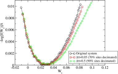
Simulations for regular lattices show a striking robustness of the entropy production Cramer function with respect to decimation. The numerically computed Cramer function $-\log f_{\Delta t}(\mathcal{W}_{t})/t$ for $1d$ chains is plotted in Figure 2 for different CGL. The figure shows that decimating $90\%$ of the system, i.e. leaving only the slowest states, the fluctuations of entropy production remain substantially the same. The result does not seem to depend on the details of the transition rates, but only on the separation of time-scales.

In the following sections, we show that the entropy production is not directly related to the properties of fast and slow states per se either, while it seems reasonable to conjecture that it is closely related to the currents flowing in the system. These are global quantities, rather than local ones, which depend on the topology and on the interplay among all transition rates, an idea that may be understood in simple terms, as follows. In the case of a random walk on a ring (a 1-dimensional lattice with periodic boundary conditions), one may write

$$\frac{W_{\omega_{0}\to\omega_{1}}W_{\omega_{1}\to\omega_{2}}...W_{\omega_{n-1}\to\omega_{n}}}{W_{\omega_{1}\to\omega_{0}}W_{\omega_{2}\to\omega_{1}}...W_{\omega_{n}\to\omega_{n-1}}}=\left(\frac{W_{forw}}{W_{back}}\right)^{m}\times\mathcal{R}$$ (8)

where $W_{forw}=W_{1\to 2}W_{2\to 3}...W_{N-1\to N}W_{N\to 1}$, $W_{back}=W_{1\to N}W_{N\to N-1}...W_{3\to 2}W_{2\to 1}$, $m$ is an integer and $\mathcal{R}\approx\mathcal{O}(1)$ is a correction term. In presence of a mean current $J>0$, one has $m=[G(t)t]$ where $G(t)$ is the current computed in the time window $(0,t)$ (i.e. $\lim_{t\to\infty}\langle G(t)\rangle=J$) and $[a]$ indicates the integer part of $a$. This leads to the relation

$$\mathcal{W}_{t}\approx G(t)\log\frac{W_{forw}}{W_{back}}+\mathcal{O}(1/t).$$ (9)

Since the decimation protocol eliminates fast states and modifies transition rates in order to leave basically unaltered the currents connecting the surviving states, the fluctuations of entropy production should not be sensibly affected by the decimation procedure. Observe, however, that this current conservation is only approximate, not exact. The modification of the current produced by the decimation can indeed be estimated analytically in simple cases, as in systems whose states form a single loop. In Appendix B, we argue that the correction should be generally small and related to the ratio of the times spent in the fast states and in the slow ones.

Figure 2: Numerically computed Cramer function for entropy production distribution in $1D$ continuous time random walks with p.b.c. In each plot a comparison among different coarse graining levels is shown. In both panels, each state of the non-decimated system may take one out of three possible average exit times: $1$ ($10\%$ of states), $0.1$ ($20\%$ of states) and $0.01$ ($70\%$ of states). In the left panel, the probability of jumping to the right is $0.4$ ($60\%$ of states) or $0.6$ ($40\%$ of states). In the right panel, the probability of jumping to the right is $0.4$. In the left frame we have $N=100$ and $t=2\cdot 10^{3}$. In the right frame we have $N=300$ and $t=10^{3}$. The numerical computation has been performed with the Gillespie algorithm Gillespie (1977), where the actual probability of a transition is the product of the transition rate by the characteristic time.

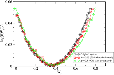
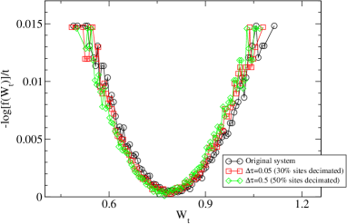
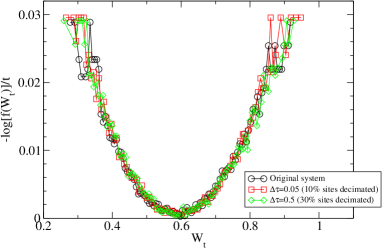
Similar results are reported in Figure 3 for 2D regular square lattices, where jumps occur among nearest neighbours: even with this topology, the fluctuations of entropy production appear not to be affected by the CGL, although the result is not as robust as in the $1D$ case. Indeed, a substantial change in entropy production can be observed if the system contains a very large number of fast states to be decimated. Nevertheless, it still is interesting to realize that the Cramer function has not changed substantially, even after $50\%$ of the original system has been decimated. Note that the square lattice topology is drastically altered by decimation: states which have not been decimated remain connected by chains of transitions, but the system is not planar nor a regular lattice anymore. Currents in this case may still be defined within a more general graph theory Schnakenberg (1976), such as that discussed in Appendix C.

Figure 3: Approximated Cramer function for entropy production distribution in continuous time random walks on a $2D$ squared lattice (nearest neighbours) with p.b.c. In each plot a comparison among different coarse graining levels is shown. In both cases the probabilities of jumping to one of the four nearest neighbours are biased to give a net current in one direction. The left and the right panels differ by the values of the exit times. Left: the states have exit times $1$ ($50\%$ of states), $0.1$ ($20\%$ of states) and $0.01$ ($30\%$ of states). Right: the states have exit times $1$ ($70\%$ of states), $0.1$ ($20\%$ of states) and $0.01$ ($10\%$ of states). In both cases $N=100$ and $t=1000$

II.3 Results on graphs with fast and slow loops

Guided by the conjecture that the fundamental ingredient for entropy production is the current flowing in a circuit, we construct Markov processes composed of independent loops joined by a single interchange state. The general structure of this graph is illustrated in Fig. 4. The main slow loop is decorated by fast loops (first level), which are on their turn decorated by faster loops (second level), etc. After decimation, one may encounter different situations:

1. the new and the old structures have the same topology, i.e. only pieces of loops have been suppressed but the number and position of loops is the same;

2. all loops of the faster (outer) level are suppressed;

3. all loops of the two fastest levels are suppressed;

4. and so on;

Loops at the same level have similar properties and, in particular, are chosen to have, or not to have, a positive entropy production, i.e. to have or not to have a preferential direction in their transition rates.

Figure 4: Sketch of a graph made of three levels of nested loops: in this example, the main level loop has no preferential direction, while the second and third levels are made of smaller loops with faster states and preferential directions.

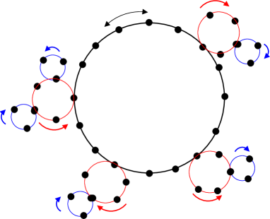
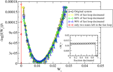
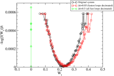
The computed Cramer function for the entropy production of the case of Figure 4 is reported in Figures 5 and 6. In Figure 5 the states of the fast loop have slightly different characteristic times, allowing a progressive decimation of the fast loop. At a decimation threshold such that the fast loop is still alive, even if made of only three states (blue curve), we are in situation 1 and the Cramer function of the entropy production is very close to that of the non-decimated system (black curve). A further increase of the decimation threshold makes the fast loop disappear: it remains with only two states and the system falls in situation 2, where the Cramer function of the entropy production has a sudden macroscopic change (red curve). The inset of Figure 5 shows $\langle\mathcal{W}_{t}\rangle$ as a function of the decimated percentage of the fast loop: neglecting a very weak growth, $\langle\mathcal{W}_{t}\rangle$ appears practically constant, until the fast loop is not reduced to a $2$-states branch. If the main loop is configured to have a non-zero current, this is what remains at that point, otherwise the fluctuations of $\mathcal{W}_{t}$ are reduced to a very narrow and symmetric peak around zero.

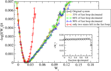
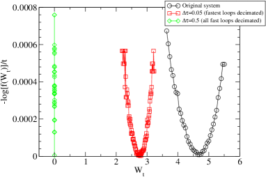
Figure 6 shows other cases with three levels of loops. The Cramer function of the entropy production always changes when a level of current-carrying loops is entirely removed.

Figure 5: Approximate Cramer function for entropy production distribution in continuous time random walks on a graph similar to that of Figure 4, with two hierarchical levels. A comparison among different coarse graining levels is shown. The main loop is made of $100$ states with average exit time $1$ and preferential direction given by balanced (left) or unbalanced (right) transition rates. In the case of unbalanced rates, they are $0.6$ toward left and $0.4$ toward right. The second level loops have $30$ states and a bias in the transition probabilities ($0.8$ vs. $0.2$) chosen to give a preferential direction, while their characteristic times range from $0.1$ to $0.7$. In all simulations $t=1000$.

Figure 6: Approximate Cramer function for entropy production distribution in continuous time random walks on the topologies of Figure 4, with three hierarchical levels of nested loops and $t=10^{4}$. In each plot a comparison among different coarse grained levels is shown. The main loop is made of $100$ states with average exit time $1$ and no preferred direction. The second level loops (each with $10$ states) have average exit time $0.1$ and a bias in the transition probability chosen to give a preferential direction. The third level loops (each with $5$ states) have average exit time $0.01$. The difference between the left and right frames is in the transition rates of this third level. Left: third level loops have a preferential direction. Right: third level loops without preferential direction.

II.4 A model from molecular biology: coarse graining of the Kinesin’s network

The examples in the previous sections suggest that the entropy production is weakly affected by the coarse graining procedure, apart from the cases in which loops contributing significantly to the entropy are destroyed and the entropy production undergoes an abrupt decrease. A natural question is whether this phenomenology is a peculiarity of the model introduced here, or similar behaviors pertain to other realistic models of non-equilibrium systems. Biochemical reactions are often characterized by non-equilibrium processes acting over different timescales and thus afford an ideal benchmark for the ideas proposed here. In this subsection, we study the effect of coarse graining on a recent network model of the kinesin motor cycle Liepelt and Lipowski (2007).

Kinesins are a common category of motor proteins Howard (2001) that are used for transport on microtubules in eucaryotic cells. Like many other non-equilibrium reactions inside cells, kinesin is powered by ATP. A number of experiments during the last decades elucidated many structural and dynamical details of this systems. In particular, it is now understood that kinesins are made of two identical heads, that walk on microtubules with a “hand-over-hand” mechanism Yildiz et al. (2004), alternating their position at the front.

The model proposed in Liepelt and Lipowski (2007) describes both the ATP-driven chemical reactions and the mechanical step in which the two heads swap. The multiple cycle structure of the reaction is given by this chemomechanical nature and by considering the fact that ATP may be burned by both heads. The scheme of the reaction and the possible transitions are illustrated in Fig.(7).

Figure 7: Scheme of the transition network of the kinesin model Liepelt and Lipowski (2007). a) Reaction network. The states, numbered from $1$ to $6$, are characterized by the two heads bound to ATP (A), ADP (D) or free. The molecules bound (or released) during the chemical transitions are shown as connected to the arrows. The dashed arrow represents the mechanical transition, in which kinesin makes its step on the microtubule. b) Kinesin network after coarse graining the fastest states, first state $2$, then state $5$. Dot-dashed arrows represent the new transitions appearing as a consequence of the coarse graining procedure.

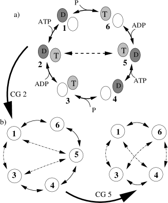
Each of the two heads may be in three different configurations: free, bound to ATP and bound to ADP, resulting in $3\times 3=9$ possible states. However, the motor is believed to work “out of phase”, i.e. states in which the two heads are in the same configuration are unlikely to be observed. This reduces the model to the $6$ states represented in the scheme of Fig. (7). Of all the possible transition among the states, only those which are consistent with experimental observations are considered in the model and shown in the diagram. Clearly, the assumptions above (in particular that of considering only $6$ states) already imply some level of coarse graining with respect to the complete problem. However, the effect of these assumptions on the entropy production is hard to determine, since it would be difficult to construct a more detailed model, from the available experimental results. We then take the model of Fig. (7) as our starting point, and study the effect of decimating the states of the system.

The transition rates of the model depend on the ADP, ATP and P concentration and on the load force $F$ of the molecular motor. Moreover, the parameters determining these rates have a slight dependence on the kind of the experiment one wants to reproduce, since different experiments work in different conditions and may use different kinds of proteins in the kinesin family. We determined the rates by choosing the parameters fitting the experiment of Ref.Carter and Cross (2005) and assumed fixed concentrations of $[ADP]=[ATP]=[P]=1\mu M$ (micromoles) for simplicity. We then consider two different cases: one without work load and one with a work force equal to $F\approx 5pN$ (piconewton). Details on the derivation of the rates and numerical values are given in Appendix (D).

In both cases (with and without load), state $2$ is the fastest and state $5$ is the second fastest. We compare then the entropy production of the complete model, of the model in which state $2$ has been adiabatically eliminated and of the model in which both $2$ and $5$ have been eliminated. The pdf of finite-time-averaged entropy production $W_{t_{max}}/t_{max}$, obtained from $10000$ realizations of trajectories of length $t_{max}$ is shown in Figure 8, without load in the left panel, with load in the right panel. Decimation of state 2 leaves the pdf unchanged. In the case without load, further decimation of state 5 changes abruptly the pdf to a close-to-zero peaked pdf.

Figure 8: Pdf’s of the entropy production per unit of time. Black curve is for the original model with 6 states. Red is after decimation of state 2. Green is after decimation of states 2 and 5. Left panel: the case without load. Right panel: the case with load.

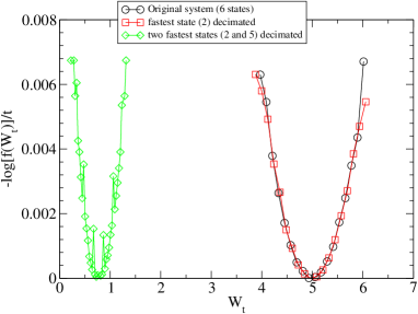
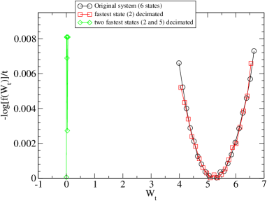
This model reproduces the same scenario of the “fast loop-slow loop” model of the previous section. The first coarse graining strongly alters the structure of the network, but its effect on the entropy production and its fluctuations is barely noticeable. Conversely, decimating one more state drastically reduces the entropy production. Notice also that the most irreversible transition in the original model is the “mechanical” transition between state $2$ and $5$, since $W_{25}/W_{52}=3\ 10^{3}$ for the load-free case and $\approx 57$ for the loaded case. In the sense specified in the next section, the information about the irreversibility of this transition is lost, when the level of coarse graining is too large.

III Tentative theory

Consider a continuous time Markov process: each state $n$ can be seen as a vertex of a graph, and transitions $n\to n^{\prime}$ with a positive rate correspond to edges (also called links) between $n$ and $n^{\prime}$. As in Lebowitz and Spohn (1999), we assume that the transition $n\to n^{\prime}$ has a positive rate whenever the inverse transition $n^{\prime}\to n$ does. As illustrated in Section 2.B, the entropy production of random walks on 1D rings is closely related to the current flowing in the ring. In this Section, we attempt to generalize this observation to generic graphs Burioni and Cassi (2005). The main tool for this purpose is a decomposition in fundamental cycles, which is illustrated in Appendix C. In the example of Figure 4, the fundamental cycles are nothing but the loops.

Let us introduce a different functional $Q_{t}$:

$$Q_{t}=\sum_{\alpha}A(\vec{C}_{\alpha})G_{\alpha}(t)$$ (10)

which depends only on a few “structural properties” of the process: the fundamental cycles $\vec{C}_{\alpha}$ (i.e. a property of the graph), their affinities $A(\vec{C}_{\alpha})$ and their fluctuating currents $G_{\alpha}$, averaged over a time interval $(0,t)$, which depend also on the transition rates.

Figure 9: Equivalence of the Cramer function for $\mathcal{W}_{t}$ and $Q_{t}$ at $t=10^{4}$. Left: random walk on a 2d lattice with same parameters as in Figure 3 (right). Right: random walk on a nested loop graph with same parameters as that in Figure 6 (right).

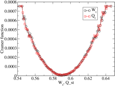
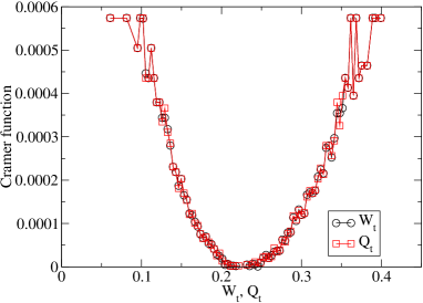
In various numerical simulations, we have verified that the fluctuations of $Q_{t}$ and those of $\mathcal{W}_{t}$ are practically indistinguishable, at large times: cf. Figure 9 for two examples. It is also known that $\langle Q_{t}\rangle=\langle\mathcal{W}_{t}\rangle$ for large times Andrieux and Gaspard (2007).

To obtain a complete theory, it remains to show that the “structural properties” are not affected by the decimation; this task can be subdivided in three steps:

1. examine the fate of fundamental cycles after decimation of one fast state; there are three possibilities: i. cycles may be destroyed, ii. transformed into different ones, iii. new cycles may be created;

2. derive the corresponding variation of affinities;

3. obtain the values of currents after decimation.

Concerning task $2$, it is easy to realize that affinities do not change in transformed cycles, while new cycles have zero affinity, so they do not contribute to the entropy production. Disappearing cycles pose, instead, a difficult question: numerical simulations show that they are usually small and that the affinity lost with their removal is equally small. At the moment, however, we do not have an analytical estimate of this quantity. Task 3 is a hard problem too: the stationary value of currents must satisfy many coupled Kirchhoff equations and depends on the properties of the whole graph. Numerical simulations suggest that average currents are not drastically influenced by our decimation procedure. One rough explanation of this fact can be given for a system $\Sigma$ with small entropy production, obtained from a perturbation of an equilibrium system $\Sigma^{0}$. Indeed, one may assume a linear relation between the affinities $A$ and the average currents $J_{\beta}$ of $\Sigma$, of the form $A(\vec{C}_{\alpha})=\sum_{\beta}L_{\alpha\beta}J_{\beta}$, with coefficients $L_{\alpha\beta}$ determined only by the properties of $\Sigma^{0}$. If the decimation procedure, which replaces $\Sigma$ with a new system $\Sigma^{\prime}$, leaves substantially unaltered the invariant probability of the surviving states, it is reasonable to assume that the decimated system $\Sigma^{\prime}$ is another small perturbation of $\Sigma^{0}$. Then, the linear relation between affinities and currents of $\Sigma^{\prime}$ retains the same coefficients $L_{\alpha\beta}$, leading to the conclusion that the currents are conserved under decimation, if affinities are.

We now discuss the consequences of decimation on cycles and their affinities. A maximal (also called “spanning”) tree $T$ is found on the original graph $G$. This tree includes all $N$ vertices (states) and only a part ($N-1$) of the original number $E$ of edges. All pairs of vertices are connected by a unique path on this tree. All edges left out from the tree (a number $\nu=E-(N-1)$) are called “chords”. A chord connecting vertices $i$ and $j$, attached to the unique path connecting $i$ and $j$ along the tree, is a closed loop. All loops generated in this way constitute the set of fundamental loops, which become “cycles” when orientation is taken into account. These fundamental cycles determine the statistics of $Q_{t}$ and therefore of $\mathcal{W}_{t}$, cf. Appendix C for the details. In the cases discussed below, the removal of a vertex using our decimation procedure preserves almost exactly the fundamental cycles and their affinities; the small variations observed are due to the possibile reduction of whole $3$-loops to $2$-loops (i.e. simple links) corresponding to a total loss of the affinity of the original $3$-loop. The impact of this unfortunate event is difficult to estimate, because it depends on the topology of the graph: the removal of a vertex may lead to a crunch of a number of loops smaller than or equal to the degree of the removed vertex. The amount of lost affinity for each reduced loop is expected to be small, since it is associated with a small loop, and correspondingly small should be the loss in current and in entropy production. It is remarkable that the exit times of states do not affect the affinities, although they can affect the currents.

Nevertheless, decimation may affect the large loops as well; a progressive and repeated removal of vertices may eventually reduce a large loop to a $2$-loop. Unfortunately, controlling these events goes beyond our mathematical ability, therefore, the size of the error in the conservation of fundamental cycles under decimation remains an open question.

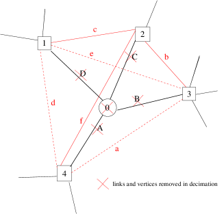
In the figures, all black objects (vertices and links) are related to the original graph, red objects are the new ones formed after decimation. Solid links are part of the maximal tree, dashed links are chords. When the state labelled by $0$ is removed, it is linked to some other states collectively denoted as $j$: $j$-states (linked to $0$) are in number of $n$. These links are broken and all pairs of states $j$ and $j^{\prime}$ (previously connected to $0$) are connected among each other with a new transition rate $W_{j->0}W_{0->j^{\prime}}/W_{0}^{0}$ (or, if the link $j-j^{\prime}$ already exists, its transition rate is updated adding that amount). We consider the simplest case where one chord at most is involved in the decimation procedure. With this assumption, three possibilities can be encountered:

Figure 10: An example of state-removal where no chords belong to the subgraph involving the removed state. Black objects (vertices and links) are relative to the original graph, red objects are formed by the decimation protocol. Solid links are part of the maximal tree, dashed links are chords.

1. new loops with no entropy production:

   The simplest case is realized when no chords connect any $j$ to $0$ and no chords connect any $j$ to any $j^{\prime}$, cf. Fig. 10 for one example. In this case, all original links $j\to 0$ ($A$, $B$, $C$ and $D$ in Fig. 10) are on the spanning tree and no links join any $j$ to any $j^{\prime}$. After the links and the central state have been removed, the red links are created (a, b, c, d, e, f in the example): they are in a number $n(n-1)/2$. A number $(n^{2}-3n+2)/2>0$ (for any $n\geq 2$) are new chords (a, d and e in the example), while the remaining $n-1$ are links of the new spanning tree (b, c and f). Therefore new loops have been created (in the example they are $3-4-2-3$ with chord a, $3-1-2-3$ with chord e and $1-2-4-1$ with chord d). It is immediate to verify that the affinity of the new loops vanishes: for instance the loop $3-1-2-3$ has forward transition rate given by $3\to 0,0\to 1,1\to 0,0\to 2,2\to 0,0\to 3$ and backward transition rate given by $3\to 0,0\to 2,2\to 0,0\to 1,1\to 0,0\to 3$ and they exactly cancel out (the exit rates are omitted, but they cancel out trivially): these new loops do not contribute to the entropy production.

   

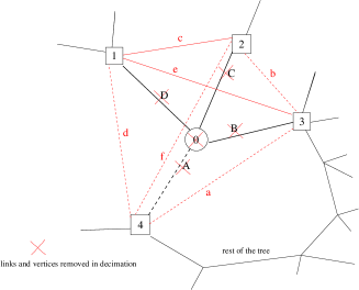
   Figure 11: An example of state-removal where a chord is removed by decimation. Black objects (vertices and links) concern the original graph, before decimation, red objects are the new ones formed after decimation. Solid links are part of the maximal tree, dashed links are chords.

2. loop-shortening:

   Another possibility (see Fig. 11) is that some link $0\to j^{*}$ is a chord in the original graph, which means that it is not in the spanning tree: e.g. link A in the example, with $j^{*}=4$. Then, state $j^{*}$ is connected to 0 through some other unique path on the tree, possibly passing through a state $j^{\prime}$ (the unique path on the tree is also represented in the figure, terminating with the link $3-0$), forming a loop $0-j^{*}-tree-j^{\prime}-0$. In this case, the decimation of state $0$ creates the link $j^{*}\to j^{\prime}$ (link “a” in the example) as a chord of the loop $j^{*}-tree-j^{\prime}-j^{*}$, which is two steps shorter than the orginal loop. It is immediate to see that the affinity of the new loop is the same as that of the old one. In this case, all new links starting from $j^{*}$, or from $j^{\prime}$, and ending in another $j$, must be chords, since $j^{*}$ and $j^{\prime}$ are joined by a unique path on the tree which has not been touched by decimation: the number of new chords is larger than in the previous case, but all their loops have zero affinities.

   There is also the possibility that the loop passing through chord $A$ is simply given by $j^{*}-0-j-j^{*}$, i.e. that it is a $3$-loop, originally belonging to the graph: this case can be put in the last category, simply exchanging the roles of the chords A and a: we call loop-crunching this case.

   

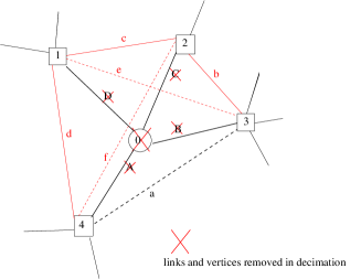
   Figure 12: An example of state-removal where a chord connects two states which are directly linked to the removed state. Black objects (vertices and links) pertain to the original graph, before decimation, red objects are formed by decimation. Solid links are part of the maximal tree, dashed links are chords.

3. loop-crunching:

   The last possibility is that some link $j\to j^{\prime}$ already existed in the original graph, which means that it is a chord of the loop $A-j-j^{\prime}-A$, cf. Fig. 12, where chord a connects states 4 and 3. In this case the removal of state $A$ leads us to crunch the $3$-loop, making it a simple link $j-j^{\prime}$ with a new transition rate. The original loop and its contribution to entropy production are then lost.

We stress that a mathematical proof of the above considerations is still lacking, although our arguments are strongly supported by numerical results.

IV Concluding remarks and open problems

In this paper we support, both numerically and theoretically, the idea that fluctuations of the entropy production are essentially insensitive to a coarse-graining based on decimation of fast states, provided that decimation does not remove fundamental loops carrying net currents. The threshold of coarse-graining level which trigger the removal of such loops is not fully understood, but our investigation suggests that entropy production fluctuations are generally quite robust with respect to decimation. Moreover, this robustness does not appear directly related to the characteristic times of the removed states. Robustness or fragility of loops appears mostly related to the global structure of the network at hand.

We applied this analysis to the network model of the biomolecule known as kinesin, discovering that no entropy production is lost if a coarse-graining from six to five states is performed. This observation is potentially interesting in biophysics, since entropy production is a fundamental property of irreversible chemical reactions, such as those fueling the kinesin motor protein. On the contrary, the decimation of the model from six to four states is catastrophic, making the model unsuitable to produce work.

More detailed studies are necessary to quantify the entropy production variations induced by coarse graining: the main missing ingredient is the evaluation of the effect of decimation on the currents of the surviving loops. This will lead to a better understanding of the role and meaning of $\mathcal{W}_{t}$ as a definition of entropy production. In particular, understanding the relation between $\mathcal{W}_{t}$ and macroscopic observable properties of the system may help in modelling non-equilibrium systems.

Appendix A The decimation procedure

In this Appendix, we summarize the coarse graining method introduced in Pigolotti and Vulpiani (2008). Consider a master equation of the form of eq. (1). Due to the Markovian nature of the process, the time spent in a generic state $n$ is exponentially distributed with average $\tau_{n}=1/W^{0}_{n}$. One may wish to decimate all states having an average permanence time smaller than a prescribed threshold $\Delta\tau$. To do that, Ref.Pigolotti and Vulpiani (2008) sets to 0 the time spent in these states. In this way, the fast states disappear from the description and transitions to them are redirected to other states with proper statistical weights. In formulae, if a state $i$ is linked to a state $j$ via a fast state $n$ that must be eliminated, the transition rate $W_{i\to j}$ from $i$ to $j$ is renormalized to yield the rate:

$$\tilde{W}_{i\to j}=W_{i\to j}+W_{i\to n}W_{n\to j}/W^{0}_{n}$$ (11)

If $W_{i\to j}=0$, the decimation creates a direct connection between the surviving states, which is reminscent of the states that disappeared from the model under consideration.

This procedure corresponds to an adiabatic approximation and is commutative, if the prescription of Pigolotti and Vulpiani (2008) is followed. Once the set of states to be decimated is determined by the threshold, they can be decimated in any order without affecting the final result, as long as the set itself is not modified during the decimation procedure. It may happen, indeed, that the permanence time of some of the states selected for decimation becomes larger than $\Delta\tau$, while other states are decimated. The recipe of Pigolotti and Vulpiani (2008) requires that this state be eventually decimated nonetheless.

Appendix B Effect of decimation on the current in a single loop

In this Appendix, we investigate the effect of decimation on the current of a single loop consisting of $N$ states. For convenience, let us rewrite the master equation:

$$\frac{d}{dt}P_{n}(t)=W_{n-1\to n}P_{n-1}+W_{n+1\to n}P_{n+1}-P_{n}(W_{n\to n+1}+W_{n\to n-1})~{},$$

with $P_{0}=P_{N}$, as:

$$\frac{d}{dt}P_{n}(t)=J_{n}-J_{n-1}$$ (12)

where the local current $J_{n}$ is given by:

$$J_{n}=P_{n-1}W_{n-1\to n}-P_{n}W_{n\to n-1}.$$ (13)

In a stationary state, the current is site-independent and one may write $J_{n}=J$. In particular, detailed balance and equilibrium hold if $J=0$. The set of equation $J_{n}=J$, together with the normalization condition $\sum_{n}P_{n}=1$, can be solved for both $J$ and the invariant measure $P_{n}^{inv}$. For instance, let us proceed iteratively, as follows:

$$P_{n} = P_{n-1}\frac{W_{n-1\to n}}{W_{n\to n-1}}-\frac{J}{W_{n\to n-1}}=$$ (14)

$$= P_{n-2}\frac{W_{n-2\to n-1}W_{n-1\to n}}{W_{n\to n-1}W_{n-1\to n-2}}-J\left(\frac{1}{W_{n\to n-1}}+\frac{1}{W_{n-1\to n-2}}\frac{W_{n-1\to n}}{W_{n\to n-1}}\right)=\dots$$

$$= P_{n}\prod\limits_{k=1}^{N}\frac{W_{k-1\to k}}{W_{k\to k-1}}-J\left(\sum\limits_{j=0}^{N-1}\frac{1}{W_{n-j\to n-j-1}}\prod\limits_{k=0}^{j}\frac{W_{n-j+k-1\to n-j+k}}{W_{n-j+k\to n-j+k-1}}\right).$$

We obtain $P_{n}$ from the last expression

$$P_{n}=\frac{-J\left(\sum\limits_{j=0}^{N-1}\frac{1}{W_{n-j\to n-j-1}}\prod\limits_{k=0}^{j}\frac{W_{n-j+k-1\to n-j+k}}{W_{n-j+k\to n-j+k-1}}\right)}{1-\prod\limits_{k=1}^{N}\frac{W_{k-1\to k}}{W_{k\to k-1}}}$$ (15)

and by means of the normalization condition $\sum P_{n}=1$, we reach the following closed expression for $J$:

$$J=\frac{\left(\prod\limits_{k=1}^{N}\frac{W_{k-1\to k}}{W_{k\to k-1}}\right)-1}{\sum\limits_{n=1}^{N}\sum\limits_{j=0}^{N-1}\frac{1}{W_{n-j\to n-j-1}}\prod\limits_{k=0}^{j}\frac{W_{n-j+k-1\to n-j+k}}{W_{n-j+k\to n-j+k-1}}}.$$ (16)

Let us now decimate one fast state, $n^{*}$ say, and consider the current. It is easy to show that the numerator is not affected by the decimation protocol defined by eq. (11). Conversely, the denominator decreases by an amount $\Delta D$ which can be espressed as follows:

$$\Delta D=D_{o}-D_{d}=\frac{1}{W_{n^{*}\to n^{*}-1}}+\sum\limits_{j=0}^{N-1}\frac{1}{W_{n^{*}+1\to n^{*}}}\prod\limits_{k=0}^{j}\frac{W_{n^{*}+k\to n^{*}+k+1}}{W_{n^{*}+k+1\to n^{*}+k}}$$ (17)

where $D_{0}$ and $D_{d}$ are the denominator in (16) for the original and the decimated system, respectively. As $\Delta D$ is positive, the current in the decimated system is larger than in the original one, the difference being

$$\Delta J=J_{d}-J=J\frac{\Delta D}{D_{0}-\Delta D}.$$ (18)

This allows us to check what happens in simple cases. For instance, eq. (17) leads to $\Delta D/D=1/N$, if all state have same left and right jump rates (the two must be different to have a non-trivial current). If the rate of the decimated state is much faster than the others, eq. (17) also shows that the correction decreases linearly with the separation of time scales, i.e. with the ratio of the average rates of the fast states and that of the other states. This is consistent with the picture of the current correction being essentially due to a rescaling of the times related to the elimination of the fast state. In other words, the magnitude of the correction seems to be always related to the ratio of the time spent in the fast state(s) and the time spent in the slow ones.

Appendix C Graphs and currents

We consider a Markovian (continuous time) process on $N$ states. The $N$ states are considered as nodes of a graph. The transitions between different states are considered as links (edges) between nodes.

C.1 Fundamental cycles

Graph theory simplifies the classification of closed loops on a graph Schnakenberg (1976), identifying a set of fundamental “cycles”. Given a graph $G$ with $N$ vertices (nodes) and $E$ edges (links between nodes), the strategy - exemplified in Figure 13 - is the following:

Figure 13: An example of graph with $5$ states and three fundamental loops: all transitions (links) have a given orientation. A possible maximal tree is the one made of only solid links, with the three dashed links representing the remaining chords, which individuate three fundamental loops. Any other possible loop, e.g. $\vec{C}=1\to 2\to 4\to 5\to 1$, can be decomposed in the sum of fundamental loops, e.g. $\vec{C}=\vec{C}_{1}+\vec{C}_{3}$.

• identify a maximal tree $T(G)$, i.e. a set containing all $N$ vertices and part of the $E$ edges, which is connected and does not contain circuits. It is easy to show that $T(G)$ has $N-1$ edges. Many maximal trees can be identified, but one suffices;

• given an arbitrary maximal tree $T(G)$, the edges of $G$ which do not belong to $T(G)$ are called chords of $T(G)$, they are in a number $\nu=E-N+1$;

• if only one chord $s_{\alpha}$, $\alpha\in[1,\nu]$, is added to $T(G)$, the new graph contains only one circuit, $C_{\alpha}$, obtained by $T(G)+s_{\alpha}$ removing all edges which are not part of the circuit; therefore, from a maximal tree, $\nu$ circuits can be generated adding the $\nu$ chords;

• the set of $\nu$ circuits obtained from the $\nu$ chords of a maximal graph is called a fundamental set of circuits, denoted by $\{C_{1},...,C_{\nu}\}$

• orientation of edges must be introduced: each edge is assumed to be oriented in an arbitrary direction, giving the oriented version of $G$, denoted as $\vec{G}$; then one can take a subgraph with oriented edges $\vec{P}$, which may have different orientations with respect to the original orientations of the edges of $\vec{G}$. The function $S_{e}(\vec{P})$ is introduced for these cases: it returns $1$ if the edge $e$ is in $\vec{P}$ and has the original orientation, $-1$ if it is in $\vec{P}$ and has opposite orientation, and $0$ if $e$ is not in $\vec{P}$.

• a cycle is an oriented circuit, e.g. $\vec{C}$; a fundamental cycle is denoted by $\vec{C}_{\alpha}$: for simplicity we always choose the orientation of a fundamental circuit to be parallel to the orientation of its chord $\alpha$, i.e. $S_{\alpha}(\vec{C}_{\alpha})=1$;

• the scalar product among cycles is defined as

  $$(\vec{C},\vec{C}_{\alpha})=S_{\alpha}(\vec{C})S_{\alpha}(\vec{C}_{\alpha})\equiv S_{\alpha}(\vec{C})$$ (19)

  where $\alpha$ is the chord which generates the circuit $C_{\alpha}$; this scalar product can only take three values: $0$, $1$ or $-1$.

• a decomposition of cycles is finally achieved: any cycle (oriented circuit) of the graph $G$ can be linearly decomposed using the fundamental set as a basis:

  $$\vec{C}=\sum_{\alpha=1}^{\nu}(\vec{C},\vec{C}_{\alpha})\vec{C}_{\alpha}$$ (20)

C.2 Currents

The current for the $\omega\to\omega^{\prime}$ transition is

$$J(\omega\to\omega^{\prime},t)=P_{\omega}(t)W_{\omega\to\omega^{\prime}}-P_{\omega^{\prime}}(t)W_{\omega^{\prime}\to\omega}.$$ (21)

The stationary state value is denoted by $J(\omega\to\omega^{\prime})$. The stationarity condition $dP_{\omega}^{inv}/dt=0$ is equivalent to

$$\sum_{\omega^{\prime}}J(\omega^{\prime}\to\omega)=0\;\;\;\;\;\;\;\forall\omega$$ (22)

which is known as Kirchhoff current law. If the transition $\omega\to\omega^{\prime}$ corresponds to the oriented edge $e$, its steady state current is also denoted as $J_{e}$.

The current (or flux) on a fundamental circuit is defined as the steady state transtion current flowing in the chord $\alpha$ in the original direction and is denoted by $J_{\alpha}$. For instance if $\alpha$ is the oriented edge corresponding to the transition $\omega\to\omega^{\prime}$, then $J_{\alpha}=J(\omega\to\omega^{\prime})$ and the flux of the associated cycle $\vec{C}_{\alpha}$ is equal to $+J_{\alpha}$.

The Kirchhoff law for the steady state guarantees that a current on any edge is the sum of the currents going through the cycles which intersect the edge, i.e.

$$J_{e}=\sum_{\alpha=1}^{\nu}S_{e}(\vec{C}_{\alpha})J_{\alpha}.$$ (23)

An edge of the graph $G$ can be oriented in a different direction with respect to the edges of the cycles, therefore the sign function $S_{e}$ is used.

The fluctuating instantaneous current $J_{\alpha}$ depends on the particular realization of the Markov process; it is measured on a chord $\alpha$ as:

$$j_{\alpha}(t)=\sum_{n=-\infty}^{+\infty}S_{\alpha}(e_{n})\delta(t-t_{n})$$ (24)

where $t_{n}$ is the time of the random transition $e_{n}$ (an oriented edge of the graph) during a trajectory of the stochastic process. In brief, $j_{\alpha}$ is the instantaneous and oriented rate of the transitions in the chord $\alpha$, for a particular realization of the process. It is a stochastic variable. Its time-average (in a finite time $t$) is denoted by

$$G_{\alpha}(t)=\frac{1}{t}\int_{0}^{t}dt^{\prime}j_{\alpha}(t^{\prime}),$$ (25)

which is still a stochastic variable. Some properties of $j_{\alpha}$ and $G_{\alpha}$ have been studied in Andrieux and Gaspard (2007).

C.3 Affinities

The affinity of a transition $\omega\to\omega^{\prime}$ is defined as

$$A(\omega\to\omega^{\prime},t)=\ln\frac{P_{\omega}(t)W_{\omega\to\omega^{\prime}}}{P_{\omega}^{\prime}(t)W_{\omega^{\prime}\to\omega}}$$ (26)

The affinity of a cycle $C$ is defined as $A(C)=\sum_{e}S_{e}(C)A(e)$, but it can also be defined as $A(C)=\sum_{e}S_{e}(C)B(e)$. where $B(\omega\to\omega^{\prime})=\ln(W_{\omega\to\omega^{\prime}}/W_{\omega^{\prime}\to\omega})$. The equivalence of these two forms is due to the fact that all $P_{\omega}(t)$ cancel out, in a cycle. For this reason the affinity of a cycle does not depend upon time, but only on the transition rates, which come from the “external physical constraints”, e.g. mechanical, chemical and thermodynamical forces.

Thanks to the decomposition of cycles described above, one can linearly decompose the affinity of any cycle in terms of affinities of a “fundamental set of cycles” $\{\vec{C}_{\alpha}\}$:

$$A(\vec{C})=\sum_{\alpha}(\vec{C},\vec{C}_{\alpha})A(\vec{C}_{\alpha})$$ (27)

where $(.,.)$ is the previously defined scalar product between cycles.

C.4 Entropy production

Having defined the Gibbs entropy as

$$\mathcal{S}(t)=-\sum_{\omega}P_{\omega}(t)\ln P_{\omega}(t),$$ (28)

its time derivative can be decomposed in two parts $d\mathcal{S}/dt=d_{e}\mathcal{S}/dt+d_{i}\mathcal{S}/dt$, where the bilinear form

$$\frac{d_{i}\mathcal{S}}{dt}=\frac{1}{2}\sum_{\omega,\omega^{\prime}}J(\omega\to\omega^{\prime},t)A(\omega\to\omega^{\prime},t)\geq 0$$ (29)

is considered as the internal entropy production, and the rest $d_{e}\mathcal{S}/dt$ is the entropy flux through the boundaries of the system of interest. In the steady state one has $d_{e}\mathcal{S}/dt=-d_{i}\mathcal{S}/dt$.

A definition of entropy production per trajectory is given by Lebowitz and Spohn Lebowitz and Spohn (1999), see Eq. (4). It depends on a particular realization, i.e. it is a stochastic variable. It can also be written as:

$$\mathcal{W}_{t}=\frac{1}{t}\sum_{e}B(e)\int_{0}^{t}dt^{\prime}j_{e}(t^{\prime}).$$ (30)

Lebowitz and Spohn have noticed that

$$\lim_{t\to\infty}\langle\mathcal{W}_{t}\rangle=\left.\frac{d_{i}\mathcal{S}}{dt}\right|_{st}$$ (31)

in the stationary state. The following relation has instead been noticed in Ref.Andrieux and Gaspard (2007):

$$\mathcal{W}_{t}=Q_{t}+R_{t}$$ (32)

with

$$Q_{t} =\sum_{\alpha}A(\vec{C}_{\alpha})G_{\alpha}(t)$$ (33)

$$R_{t} =\frac{1}{t}\sum_{e\neq{\alpha}}B(e)\left[\int_{0}^{t}dt^{\prime}\left(j_{e}(t^{\prime})-\sum_{\alpha}S_{e}(\vec{C}_{\alpha})j_{\alpha}(t^{\prime})\right)\right].$$ (34)

The $Q_{t}$ term is the contribution due to the fundamental set of cycles. The “remainder” $R_{t}$ has zero average (thanks to the Kirchhoff law Eq. (23)). This implies that

$$\left.\frac{d_{i}\mathcal{S}}{dt}\right|_{st}=\lim_{t\to\infty}\langle\mathcal{W}_{t}\rangle=\lim_{t\to\infty}\langle Q_{t}\rangle=\sum_{\alpha}A(\vec{C}_{\alpha})J_{\alpha},$$ (35)

since

$$\lim_{t\to\infty}\langle G_{\alpha}(t)\rangle=\lim_{t\to\infty}\frac{1}{t}\left\langle\int_{0}^{t}j_{\alpha}(t^{\prime})dt^{\prime}\right\rangle=J_{\alpha}.$$ (36)

Numerical comparison of the fluctuations of $Q_{t}$ and those of $\mathcal{W}_{t}$ show that they have identical Cramer functions (see Figure 9), in many examples of continuous time Markov processes.

From eq. (21), detailed balance, with respect to the invariant measure, is equivalent to

$$J(\omega\to\omega^{\prime})=0\;\;\;\;\;\forall(\omega\to\omega^{\prime}),$$ (37)

which implies that the probability of any trajectory is equal to the probability of its time reversal. Detailed balance also implies that the flux on any cycle vanishes, $J_{\alpha}=0$, and that affinities vanish on a single edge as well as on any cycle, eg. $A(\vec{C}_{\alpha})=0$. As an immediate consequence, the internal entropy production vanishes:

$$\left.\frac{d_{i}\mathcal{S}}{dt}\right|_{st}=0.$$ (38)

Appendix D Appendix: parameters in the kinesin model

As sketched in Section II.4, the rates in the kinesin network model of Ref.Liepelt and Lipowski (2007) are adjusted to the parameters obtained by specific experiments. Moreover, they depend on the concentrations of the chemical species entering the reaction (ADP, ATP and P), as well as on the load force $F$. More formally, one has:

$$W_{i\to j}=k_{ij}\ I_{ij}([X])\ \Phi_{ij}(F)$$ (39)

where the $k$’s are the experiment-specific parameters. The functions $I_{ij}$ and $\Phi_{ij}$ express the dependence of the reaction rates on a generic chemical species $X$ and/or on the load force $F$. If the transition from $i$ to $j$ does not involve chemical binding, we define $I_{ij}\equiv 1$.

Assuming diluted solutions, all reactions are diffusion-limited, so that we can assume $I([X])\sim[X]$. The $\Phi$’s are adimensional functions, with the convention $\Phi(0)=1$. Theoretical considerations lead to $\Phi_{ij}(F)=\Phi_{ji}(F)=2/(1+e^{\chi_{ij}\bar{F}})$ for the chemical transitions, i.e. all but those between states $2$ and $5$. Mechanical transitions are parametrized by $\Phi_{25}=e^{-\theta\bar{F}}$ and $\Phi_{52}=e^{(1-\theta)\bar{F}}$. The $\chi$’s and $\theta$ are additional parameters obtained by experiments, while $\bar{F}=lF/kT$ is the adimensional force ($l\approx 8nm$ being the average kinesin step length and $k$ the Boltzmann constant). With these choices, the $k$’s are dimensionally different depending on whether they multiply a concentration (dimensions of rate divided by concentration, $[(\mu M\ s)^{-1}]$) or not (dimension of a rate, $[s^{-1}]$).

The parameters we used in the simulations are derived from those reproducing the results of the experiment Carter and Cross (2005):

• The values of $k$’s describing the experiment Carter and Cross (2005) according to Liepelt and Lipowski (2007) are $k_{25}=3\cdot 10^{5}$, $k_{52}=0.24$, $k_{12}=k_{45}=2.0$, $k_{21}=100$, $k_{56}=k_{61}=k_{23}=k_{34}=100$, $k_{65}=k_{32}=0.02$, $k_{16}=k_{43}=0.02$. The upper and lower cycle in Fig. 7 are assumed to have same parameters, apart from the transition from $5$ to $4$, which is determined from theoretical considerations as $k_{54}=k_{21}(k_{52}/k_{25})^{2}=6.4\ 10^{-11}$.

• Typical concentrations in the experiment are $0.5\mu M$. For simplicity, we assume all of them to be kept constant and equal to $[P]=[ADP]=[ATP]=1\mu M$.

• The mechanical parameters reproducing the results of experiment Carter and Cross (2005) are: $\theta=0.65$, $\chi_{12}=\chi_{45}=0.25$, $\chi_{23}=\chi_{56}=0.15$, $\chi_{34}=\chi_{61}=0.15$. In all cases, we have $\chi_{ij}=\chi_{ji}$.

In section II.4, we considered two instances of the model. The first one is without load, $F=0$. In this case and with the assumptions above, it is easy to obtain the transition rates: all the $\Phi$’s and concentrations are equal to $1$, so from Eq. (39) we obtain $W_{i\to j}=k_{ij}$: the rates are just the $k$’s listed above.

About the load case, the unit of the adimensional force is equal to $kT/l\approx 0.5pN$. Experiments are performed with forces of the order of piconewton. We took a value $\bar{F}=10$: substituting this value in the expression for the $\Phi$’s leads to the following values of the transition rates, which are those used in the simulations of the model with load: $W_{2\to 5}=451$, $W_{5\to 2}=7.95$, $W_{1\to 2}=W_{4\to 5}=0.3$, $W_{2\to 1}=15$, $W_{5\to 6}=W_{6\to 1}=W_{2\to 3}=W_{3\to 4}=36.5$, $W_{6\to 5}=W_{3\to 2}=0.007$, $W_{1\to 6}=W_{4\to 3}=0.007$, $W_{5\to 4}=0.5\ 10^{-11}$.

Appendix E List of the main symbols

• $W_{i\to j}$ is the transition rates from $i$ to $j$

• $W_{i}^{0}$ is the exit rate from state $i$

• $\tau_{i}=1/W_{i}^{0}$ is the characteristic time of state $i$

• $P_{n}(t)$ is the probability of being in $n$ at time $t$

• $P_{n}^{inv}$ is the invariant probability of being in $n$

• $\Delta\tau$ is the time threshold for decimation

• $\tilde{W}_{i\to j}$ are the new transition rates in the decimated process

• $\mathcal{W}_{t}$ is the Lebowitz-Spohn entropy production integrated on time $t$ and divided by $t$

• $C()$ is the Cramer’s function of the entropy production

• $f(\mathcal{W}_{t})\sim e^{-tC(\mathcal{W}_{t})}$ is the probability density of $\mathcal{W}_{t}$

• $C_{\Delta\tau}(\mathcal{W}_{t})$ is the Cramer function in the decimated process with a time threshold $\Delta\tau$.

• $\vec{C}_{\alpha}$ is an oriented cycle of the graph

• $G_{\alpha}(t)$ is the current on cycle $\alpha$ averaged on a finite time $t$

• $A(\vec{C}_{\alpha})$ is the affinity associated to the oriented cycle $\vec{C}_{\alpha}$.

References

- Ma (1985) S.-K. Ma, Statistical Mechanics (World Scientific, 1985).
- Kadanoff (2000) L. Kadanoff, Statistical Physics: Statics, Dynamics and Remormalization (World Scientific, 2000).
- Castiglione et al. (2008) P. Castiglione, M. Falcioni, A. Lesne, and A. Vulpiani, Chaos and coarse graining in Statistical Mechanics (Cambridge University Press, 2008).
- Bonaldi et al. (2009) M. Bonaldi, L. Conti, P. D. Gregorio, L. Rondoni, G. Vedovato, A. Vinante, M. Bignotto, M. Cerdonio, P. Falferi, N. Liguori, et al., Phys. Rev. Lett. 103, 010601 (2009).
- Gregorio et al. (2009) P. D. Gregorio, L. Rondoni, M. Bonaldi, and L. Conti, J. Stat. Mech. p. P10016 (2009).
- Evans et al. (1993) D. J. Evans, E. G. D. Cohen, and G. P. Morriss, Phys. Rev. Lett. 71, 2401 (1993).
- Gallavotti and Cohen (1995) G. Gallavotti and E. G. D. Cohen, J. Stat. Phys. 80, 931 (1995).
- Jarzynski (1997) C. Jarzynski, Phys. Rev. Lett. 78, 2690 (1997).
- Lebowitz and Spohn (1999) J. L. Lebowitz and H. Spohn, J. Stat. Phys. 95, 333 (1999).
- Rahav and Jarzynski (2007) S. Rahav and C. Jarzynski, J. Stat. Mech. p. P09012 (2007).
- Pigolotti and Vulpiani (2008) S. Pigolotti and A. Vulpiani, J. Chem. Phys. 128, 154114 (2008).
- de Groot and Mazur (1984) S. R. de Groot and P. Mazur, Non-equilibrium thermodynamics (Dover Publications, New York, 1984).
- Marini Bettolo Marconi et al. (2008) U. Marini Bettolo Marconi, A. Puglisi, L. Rondoni, and A. Vulpiani, Phys. Rep. 461, 111 (2008).
- Gillespie (1977) D. T. Gillespie, J. Phys. Chem. 81, 2340 (1977).
- Schnakenberg (1976) J. Schnakenberg, Rev. Mod. Phys. 48, 571 (1976).
- Liepelt and Lipowski (2007) S. Liepelt and R. Lipowski, Phys. Rev. Lett. 98, 258102 (2007).
- Howard (2001) J. Howard, Mechanics of Motor Proteins and the Cytoskeleton (Sinauer, 2001).
- Yildiz et al. (2004) A. Yildiz, M. Tomishige, R. D. Vale, and P. R. Selvin, Science 303, 676 (2004).
- Carter and Cross (2005) N. J. Carter and R. A. Cross, Nature (London) 435, 308 (2005).
- Burioni and Cassi (2005) R. Burioni and D. Cassi, J. Phys. A 38, R45 (2005).
- Andrieux and Gaspard (2007) D. Andrieux and G. Gaspard, J. Stat. Phys. 127, 107 (2007).