Abstract:

We present a determination of the parton distributions of the nucleon from a global set of hard scattering data using the NNPDF methodology: NNPDF2.0. Experimental data include deep–inelastic scattering with the combined HERA-I dataset, fixed target Drell-Yan production, collider weak boson production and inclusive jet production. Next–to–leading order QCD is used throughout without resorting to $K$–factors. We present and utilize an improved fast algorithm for the solution of evolution equations and the computation of general hadronic processes. We introduce improved techniques for the training of the neural networks which are used as parton parametrization, and we use a novel approach for the proper treatment of normalization uncertainties. We assess quantitatively the impact of individual datasets on PDFs. We find very good consistency of all datasets with each other and with NLO QCD, with no evidence of tension between datasets. Some PDF combinations relevant for LHC observables turn out to be determined rather more accurately than in any other parton fit.

1 Introduction

Over the last several years, we have developed a novel approach [1] to the determination of parton distribution functions (PDFs), which combines a Monte Carlo representation of the probability measure in the space of PDFs with the use of neural networks as a set of unbiased basis functions (the NNPDF methodology, henceforth). The method was developed, refined, and applied to problems of increasing complexity: the parametrization of a single structure function [1], of several structure functions [2] and the determination of the nonsinglet parton distribution [3]. Eventually, in Ref. [4] a first complete set of parton distributions was constructed, using essentially all the then–available deep–inelastic scattering (DIS) data. This parton set, NNPDF1.0, included five independent parton distributions (the two lightest flavours and antiflavours and the gluon). It was then extended in Refs. [5, 6] to also include an independent parametrization of the strange and antistrange quarks, with heavier flavours determined dynamically (NNPDF1.2 parton set). All NNPDF parton sets are available through the LHAPDF interface [7, 8]. In these works, as well as in studies for the HERA–LHC workshop [9], it was shown that PDFs determined using the NNPDF methodology enjoy several desirable features: the Monte Carlo behaves in a statistically consistent way (e.g., uncertainties scale as expected with the size of the sample) [4, 6]; results are demonstrably independent of the parton parametrization [4, 6]; PDFs behave as expected upon the addition of new data (e.g. uncertainties expand when data are removed and shrink when they are added unless the new data is incompatible with the old) [4, 9] and results are even stable upon the addition of new independent PDF parametrizations [5, 4].

With PDF uncertainties under control, detailed precision physics studies become possible, such as for instance the determination of CKM matrix elements [6]. However, the requirements of precision physics are such that it is mandatory to exploit all the available information in PDF determination. Specifically, it has been known for a long time (see Ref. [4] for references to the earlier literature) that DIS data are insufficient to determine accurately many aspects of PDFs, such as the flavour decomposition of the quark and antiquark sea or the gluon distribution, especially at large $x$: indeed, the current state–of–the–art PDF determinations, such as CTEQ6.6 [10] and MSTW2008 [11] are based on global fits, in which hadronic data are included along with DIS data.

In this paper we present a PDF determination using NNPDF methodology based on a global fit. The data used for fitting include, on top of all the data used in Ref. [6] (DIS data and “dimuon” charm neutrino production data) also hadronic data, specifically Drell–Yan (DY), W and Z production and Tevatron inclusive jets. We also replace the separate ZEUS and H1 datasets with the recently published HERA-I combined dataset [12]. The dataset used in this parton determination is thus comparable in variety and size (and is in fact slightly larger) to that used by the CTEQ [10] and MSTW groups [11].

The PDF determination presented here is based on a consistent use of NLO QCD. This is novel in the context of a global parton determination: indeed, in other parton fits such as Refs. [10, 11] only DIS data are treated using fully NLO QCD, while several sets of hadronic data are treated using LO theory improved through $K$–factors. The main bottleneck in the use of NLO theory for hadronic processes is the speed in the computation of hadron–level observables, which requires a convolution of the PDF of both incoming hadrons with parton–level cross sections. The use of Mellin–space techniques (as e.g. in Ref. [13]) solves this problem, but at the cost of limiting the flexibility of the acceptable PDF parametrization: specifically, the very flexible neural network method of Refs. [4, 6] parametrizes PDFs in $x$ space. Efficient fast methods to overcome this hurdle have been suggested (see [14], in [15]), based on the idea of precomputing and storing the convolution with a set of basis functions over which any PDF can be expanded. These methods have been implemented in fast public codes for specific processes, such as FastNLO [16] for jet production, and very recently in a general–purpose interface APPLGRID [17].

In this paper, we use similar ideas to fully exploit the powerful parton evolution method introduced in Ref. [3], based on the convolution of PDFs with a pre–computed kernel, determined using Mellin–space techniques. This gives us a new approach, which we call the FastKernel method, which we use both for parton evolution, and for the computation of DIS and DY physical observables. The FastKernel method leads to a considerable increase in speed in comparison to Refs. [4, 6] for DIS data, and it makes possible for the first time to use exact NLO theory for DY in a global parton fit.

Thanks to the FastKernel method, we are able to produce a first fully NLO global parton set using NNPDF methodology: the NNPDF2.0 parton set. This parton determination enjoys the same desirable features of the previous NNPDF1.0 and NNPDF1.2 PDF sets, with which in particular it is fully compatible, though uncertainties are now significantly smaller, and in fact sometimes also rather smaller than those of other existing global fits. Thanks to the use of a Monte Carlo methodology, it is possible to perform a detailed comparison of NNPDF2.0 PDFs with those of previous NNPDF fits, and in particular to assess the impact of the various new aspects of this parton determination, both due to improved methodology and the use of more precise data and a wider dataset. Perhaps the most striking feature of the NNPDF2.0 parton determination is the fact that it is free of tension between different datasets and NLO QCD: in fact, whereas the addition of new data leads to sizable error reduction, we do not find any evidence of any individual dataset being incompatible with the others, nor for the distribution of fit results to contradict statistical expectations. Specifically, any combination or subset of the data included in the global analysis can be fitted using the same methodology, and results obtained fitting to various subsets of data are all compatible with each other.

Whereas we refer to the previous NNPDF papers [4, 6] for a general introduction to the NNPDF methodology, all the new aspects of the NNPDF2.0 parton determination are fully documented in this paper. In particular, in Sect. 2 we discuss the features of the new data used here, and specifically the kinematics of DY and jet data. In Sect. 3 we discuss in detail the FastKernel method, and its application to parton evolution and the computation of DIS and DY observables. In Sect. 4 we discuss several improvements in the techniques that ensure that the quality of the fit to different data is balanced, which are made necessary by the greater complexity of the NNPDF2.0 dataset.

Readers who are not interested in the details of parton determination and the NNPDF methodology, and mostly interested in PDF use should skip directly to Sect. 5, where our results are presented. In this section, after comparing the NNPDF2.0 PDF set both with previous NNPDF sets and with current MSTW and CTEQ PDFs, we turn to a series of studies of its features. Specifically, we study possible non–gaussian behaviour of our results by comparing standard deviations with confidence level intervals; we assess one by one the impact on the new fit of the aforementioned improved fitting method, of an improved treatment of normalization uncertainties discussed elsewhere and used here [18], of the new combined HERA data, and of the addition of either jet or DY data; we discuss the impact of positivity constraints; and we discuss the dependence of our results on the value of $\alpha_{s}$.

Finally, in Sect. 6 we perform some preliminary studies of the phenomenological implications of this PDF determination: after briefly summarizing the quality of the agreement between data and theory for the processes used in the fit, we reassess the implication of our improved strangeness determination for the so–called NuTeV anomaly [19, 20], and we discuss some LHC standard candles. Some statistical tools and a brief summary of factorization and kinematics for the DY process are collected in appendices.

2 Experimental data

The NNPDF2.0 parton determination includes both deep-inelastic (DIS) data and hadronic Tevatron data for fixed–target Drell-Yan and collider weak vector boson and inclusive jet production. The DIS dataset only differs from that used in the previous NNPDF1.2 [6] PDF determination in the replacement of separate H1 and ZEUS datasets with the combined HERA-I dataset of Ref. [12].

The treatment of experimental data in the present fit follows Ref. [4], with the exception of normalization uncertainties, which are treated using the improved method presented in Ref. [18], the so-called $t_{0}$ method. All information on correlated systematic errors,when available, is included in our fit.

In this section first we introduce the dataset and the way we construct the experimental covariance matrix. Then we discuss the details of the new datasets used in the NNPDF2.0 analysis as compared to previous work, and finally we show how the Monte Carlo generation of replicas of experimental data is used to construct the sampling of the available experimental information.

2.1 Dataset, uncertainties and correlations

The dataset used for the present fit is summarized in Table 1, where experimental data is separated into DIS data, fixed target Drell-Yan production, collider weak boson production and inclusive jet production. For each dataset we provide the number of points both before and after kinematic cuts, and their kinematic ranges. The same kinematical cuts as in [4] are applied to DIS data, while no cuts are applied to the hadronic data: we impose $Q^{2}\geq Q_{0}^{2}=m_{c}^{2}=2$ GeV² and $W^{2}\geq 12.5$ GeV².

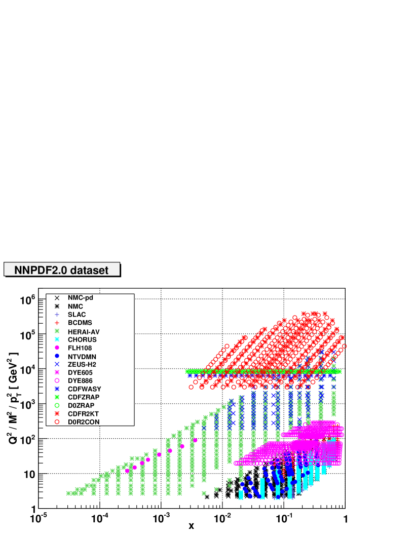
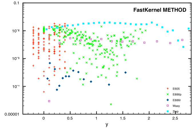
For hadronic data we use the LO partonic kinematics to estimate the effective range of Bjorken-$x$ which eaech dataset span (see Sect. 2.2 below for a definition of the pertinent kinematic variables). eeIn Fig. 1 we show a scatter plot of the data, which demonstrates that the kinematic coverage is now much more extended than in the DIS–only NNPDF1.2 fit.

The DIS data of Table 1 and Fig. 1 differ from the NNPDF1.2 set because of the replacement of all ZEUS and H1 data from the HERA-I run with the combined set of Ref. [12]. The combined HERA-I dataset has a better accuracy than that expected on purely statistical grounds from the combination of previous H1 and ZEUS data because of the reduction of systematic errors from the cross-calibration of the two experiments. These data are given with 110 correlated systematic uncertainties and three correlated procedural uncertainties, which we fully include in the covariance matrix. The remaining DIS data are the same as in Ref. [6], to which we refer for further details. Hadronic data are discussed in greater detail in Sect. 2.2 below.

In Table 2 we show the percentage average experimental uncertainties for each dataset, where uncertainties are separated into statistical (which includes uncorrelated systematic), correlated systematic and normalization uncertainties. As in the case of Table 1, for the DIS datasets we provide the values with and without kinematical cuts, if different.

Figure 1: Experimental data which enter the NNPDF2.0 analysis (Table 1). For hadronic data, the values of $x_{1}$ and $x_{2}$ determined by leading order partonic kinematics (Eqs. (3), (4) and (12)) are plotted (two values per data point).

The covariance matrix is computed for all the data included in the fit, as discussed in Ref. [4]. An important difference in comparison to [4] is the improved treatment of normalization uncertainties. Following [18], the covariance matrix for each experiment is computed from the knowledge of statistical, systematic and normalization uncertainties as follows:

$$({\rm cov_{t_{0}}})_{IJ}=\left(\sum_{l=1}^{N_{c}}\sigma_{I,l}\sigma_{J,l}+\delta_{IJ}\sigma_{I,s}^{2}\right)F_{I}F_{J}+\left(\sum_{n=1}^{N_{a}}\sigma_{I,n}\sigma_{J,n}+\sum_{n=1}^{N_{r}}\sigma_{I,n}\sigma_{J,n}\right)F_{I}^{(0)}F_{J}^{(0)}\ ,$$ (1)

where $I$ and $J$ run over the experimental points, $F_{I}$ and $F_{J}$ are the measured central values for the observables $I$ and $J$, and $F_{I}^{(0)}$, $F_{J}^{(0)}$ are the corresponding observables as determined from some previous fit.

The uncertainties, given as relative values, are: $\sigma_{I,l}$, the $N_{c}$ correlated systematic uncertainties; $\sigma_{I,n}$, the $N_{a}$ ($N_{r}$) absolute (relative) normalization uncertainties; $\sigma_{I,s}$ the statistical uncertainties (which includes uncorrelated systematic uncertainties). The values of $F^{(0)}_{I}$ have been determined iteratively, by repeating the fit and using for $F^{(0)}_{I}$ at each iteration the results of the previous fit. In practice, convergence of the procedure is very fast and the final values of $F^{(0)}_{I}$ used in Eq. (1) do not differ significantly from the final NNPDF2.0 fit results. Note that thanks to this iterative procedure, normalization uncertainties can be included in the covariance matrix as all other systematics and therefore they do not require the fitting of shift parameters.

The use of this treatment of normalization uncertainties is necessary because of the presence in the fit of data affected by disparate normalization uncertainties: indeed, the simpler method used in Refs. [1]-[6] is only accurate [18] when all normalization uncertainties have a similar size.

Deep-Inelastic scattering
Experiment	Set	Ref.	$N_{\rm dat}$	$x_{\rm min}$	$x_{\rm max}$	$Q^{2}_{\rm min}$ [GeV2]	$Q^{2}_{\rm max}$ [GeV2]
NMC-pd			260 (153)
	NMC-pd	[21]	260 (153)	0.0015 (0.008)	0.68	0.2 (2.2)	99.0
NMC			288 (245)
	NMC	[22]	288 (245)	0.0035 (0.0056)	0.47	0.8 (2.1)	61.2
SLAC			422 (93)
	SLACp	[23]	211 (47)	0.07	0.85 (0.55)	0.58 (2.0)	29.2
	SLACd	[23]	211 (46)	0.07	0.85 (0.55)	0.58 (2.0)	29.1
BCDMS			605 (581)
	BCDMSp	[24]	351 (333)	0.07	0.75	7.5	230.0
	BCDMSd	[24]	254 (248)	0.07	0.75	8.8	230.0
HERAI-AV			741 (608)
	HERA1-NCep	[12]	528 (395)	$6.2\,10^{-7}$ ($3.1\,10^{-5}$)	0.65	0.045 (2.7)	30000
	HERA1-NCem	[12]	145	$1.3\,10^{-3}$	0.65	90.000	30000
	HERA1-CCep	[12]	34	0.008	0.4	300.0	15000
	HERA1-CCem	[12]	34	0.013	0.4	300.0	30000
CHORUS			1214 (942)
	CHORUSnu	[25]	607 (471)	0.02	0.65	0.3 (2.0)	95.2
	CHORUSnb	[25]	607 (471)	0.02	0.65	0.3 (2.0)	95.2
FLH108			8
	FLH108	[26]	8	0.00028	0.0036	12.0	90.000
NTVDMN			90 (84)
	NTVnuDMN	[27, 28]	45 (43)	0.027	0.36	1.1 (2.2)	116.5
	NTVnbDMN	[27, 28]	45 (41)	0.021	0.25	0.8 (2.1)	68.3
ZEUS-H2			127
	Z06NC	[29]	90	$5\,10^{-3}$	0.65	200	$3\,10^{5}$
	Z06CC	[30]	37	0.015	0.65	280	$3\,10^{5}$
Fixed Target Drell-Yan production
Experiment	Set	Ref.	$N_{\rm dat}$	$\left[y/x^{F}_{\rm min},y/x^{F}_{\rm max}\right]$	$\left[x_{\rm min},x_{\rm max}\right]$	$M^{2}_{\rm min}$ [GeV2]	$M^{2}_{\rm max}$ [GeV2]
DYE605			119
	DYE605	[31]	119	$\left[-0.20,0.40\right]$	$\left[0.14,0.65\right]$	50.5	286
DYE866			390
	DYE866p	[32, 33]	184	$\left[0.0,0.78\right]$	$\left[0.017,0.87\right]$	19.8	251.2
	DYE866r	[34]	15	$\left[0.05,0.53\right]$	$\left[0.025,0.56\right]$	21.2	166.4
Collider vector boson production
Experiment	Set	Ref.	$N_{\rm dat}$	$\left[y_{\rm min},y_{\rm max}\right]$	$\left[x_{\rm min},x_{\rm max}\right]$	$M^{2}_{\rm min}$ [GeV2]	$M^{2}_{\rm max}$ [GeV2]
CDFWASY			13
	CDFWASY	[35]	13	$\left[0.10,2.63\right]$	$\left[2.9\,10^{-3},0.56\right]$	6463	6463
CDFZRAP			29
	CDFZRAP	[36]	29	$\left[0.05,2.85\right]$	$\left[2.9\,10^{-3},0.80\right]$	8315	8315
D0ZRAP			28
	D0ZRAP	[37]	28	$\left[0.05,2.75\right]$	$\left[2.9\,10^{-3},0.72\right]$	8315	8315
Collider inclusive jet production
Experiment	Set	Ref.	$N_{\rm dat}$	$\left[y_{\rm min},y_{\rm max}\right]$	$\left[x_{\rm min},x_{\rm max}\right]$	$p^{2}_{T,\rm min}$ [GeV2]	$p^{2}_{T,\rm max}$ [GeV2]
CDFR2KT			76
	CDFR2KT	[38]	76	$\left[0.05,1.85\right]$	$\left[4.6\,10^{-3},0.90\right]$	3364	$3.7\,10^{5}$
D0R2CON			110
	D0R2CON	[39]	110	$\left[0.20,2.20\right]$	$\left[3.1\,10^{-3},0.97\right]$	3000	$3.4\,10^{5}$
Total
Experiment			$N_{\rm dat}$	$x_{\rm min}$	$x_{\rm max}$	$Q^{2}_{\rm min}$ [GeV2]	$Q^{2}_{\rm max}$ [GeV2]
TOTAL			4520 (3415)	$3.1\,10^{-5}$	0.97	2.0	$3.7\,10^{5}$

Table 1: Experimental datasets included in the NNPDF2.0 global analysis. For DIS experiments we provide in each case the number of data points and the ranges of the kinematical variables before and after (in parenthesis) kinematical cuts. For hadronic data we show the ranges of parton $x$ covered for each set (denoted by $\left[x_{\rm min},x_{\rm max}\right]$), determined using leading order parton kinematics (Eqs. (3), (4) and (12)). Note that hadronic data are unaffected by kinematic cuts. The values of $x_{\rm min}$ and $Q^{2}_{\rm min}$ for the total dataset hold after imposing kinematic cuts.

Deep-Inelastic scattering
Set	$\left\langle\sigma_{\rm stat}\right\rangle$ (%)	$\left\langle\sigma_{\rm sys}\right\rangle$ (%)	$\left\langle\sigma_{\rm norm}\right\rangle$ (%)	$\left\langle\sigma_{\rm tot}\right\rangle$ (%)
NMC-pd	2.0 (1.7)	0.4 (0.2)	0.0	2.1 (1.8)
NMC	3.7 (3.7)	2.3 (2.1)	2.0	5.0 (4.9)
SLACp	2.7 (3.8)	0.0	2.2	3.6 (4.5)
SLACd	2.5 (3.4)	0.0	1.8	3.1 (3.9)
BCDMSp	3.2 (3.1)	2.0 (1.7)	3.2	5.5 (5.2)
BCDMSd	4.5 (4.4)	2.3 (2.1)	3.2	6.6 (6.4)
HERA1-NCep	4.0	1.9 (1.5)	0.5	4.7 (4.5)
HERA1-NCem	10.9	1.9	0.5	11.2
HERA1-CCep	11.2	2.1	0.5	11.4
HERA1-CCem	22.3	3.5	0.5	22.7
CHORUSnu	4.2 (4.1)	6.4 (5.8)	7.9 (7.6)	11.2 (10.6)
CHORUSnb	13.8 (14.9)	7.8 (7.5)	8.7 (8.2)	18.7 (19.1)
FLH108	47.2	53.3	5.0	71.9
NTVnuDMN	16.2 (16.0)	0.0	2.1	16.3 (16.2)
NTVnbDMN	26.6 (26.4)	0.0	2.1	26.7 (26.5)
Z06NC	3.8	3.7	2.6	6.4
Z06CC	25.5	14.3	2.6	31.9
Fixed Target Drell-Yan production
Set	$\left\langle\sigma_{\rm stat}\right\rangle$ (%)	$\left\langle\sigma_{\rm sys}\right\rangle$ (%)	$\left\langle\sigma_{\rm norm}\right\rangle$ (%)	$\left\langle\sigma_{\rm tot}\right\rangle$ (%)
DYE605	16.6	0.0	15.0	22.6
DYE866p	20.4	0.0	6.5	22.1
DYE866r	3.6	1.0	0.0	3.8
Collider vector boson production
Set	$\left\langle\sigma_{\rm stat}\right\rangle$ (%)	$\left\langle\sigma_{\rm sys}\right\rangle$ (%)	$\left\langle\sigma_{\rm norm}\right\rangle$ (%)	$\left\langle\sigma_{\rm tot}\right\rangle$ (%)
CDFWASY	4.2	4.2	0.0	6.0
CDFZRAP	5.1	6.0	6.0	11.5
D0ZRAP	7.6	0.0	6.1	10.2
Collider inclusive jet production
Set	$\left\langle\sigma_{\rm stat}\right\rangle$ (%)	$\left\langle\sigma_{\rm sys}\right\rangle$ (%)	$\left\langle\sigma_{\rm norm}\right\rangle$ (%)	$\left\langle\sigma_{\rm tot}\right\rangle$ (%)
CDFR2KT	4.5	21.1	5.8	23.0
D0R2CON	4.4	14.3	6.1	16.8

Table 2: Average statistical, systematic and normalization uncertainties for each of the experimental datasets included in NNPDF2.0. Uncorrelated systematic uncertainties are considered as part of the statistical uncertainty. All uncertainties are given in percentage. Details on the number of points and the kinematics of each dataset are provided in Table 1. For DIS experiments average uncertainties are given both before and (in parenthesis) after cuts.

2.2 New experimental observables

The hadronic observables used in the NNPDF2.0 PDF determination correspond to three classes of processes: Drell–Yan production in fixed target experiments, collider weak vector boson production, and collider inclusive jet production. For each type of process we briefly introduce the leading order structure of the observables and kinematics used in Tab. 1 and Fig. 1, then discuss the features of the data. Full NLO expressions for Drell-Yan observables are summarized in Appendix B, and their fast implementation is presented in detail in Sect. 3. For jet observables, we interfaced our code with FastNLO [16], by direct inclusion of the precomputed tables from this reference, to which we refer for explicit expressions for the cross–sections.

2.2.1 Drell-Yan production on a fixed target

We consider data for the double–differential distribution in $M$, the invariant mass of the Drell-Yan lepton pair, and either the rapidity of the pair $y$ or Feynman $x_{F}$, respectively defined in terms of the hadronic kinematics as

$$y\equiv{{1}\over{2}}\ln{{q_{0}+q_{z}}\over{q_{0}-q_{z}}};\quad x_{F}\equiv{{2q_{z}}\over{\sqrt{s}}},$$ (2)

where $\sqrt{s}$ is the hadron–hadron center-of-mass energy, $q$ is the four-vector of the Drell-Yan pair and $q_{z}$ is its projection on the longitudinal axis.

At leading order, the parton kinematics is entirely fixed in terms of hadronic variables by

$$x_{1}^{0}=\sqrt{\tau}e^{y}={{M}\over{\sqrt{s}}}e^{y}\ ,\qquad x_{2}^{0}=\sqrt{\tau}e^{-y}={{M}\over{\sqrt{s}}}e^{-y}\ ,$$ (3)

or equivalently

$$x_{1}^{0}={{1}\over{2}}\left(x_{F}+\sqrt{x_{F}^{2}+4\tau}\right),\qquad x_{2}^{0}={{1}\over{2}}\left(-x_{F}+\sqrt{x_{F}^{2}+4\tau}\right)\ .$$ (4)

The corresponding inverse relations are

$$\tau=x_{1}^{0}x_{2}^{0};\quad M^{2}=sx_{1}^{0}x_{2}^{0}$$ (5)

and

$$y={{1}\over{2}}\ln{{x_{1}^{0}}\over{x_{2}^{0}}};\qquad x_{F}\equiv x_{1}^{0}-x_{2}^{0}$$ (6)

At leading order, the $y$ or $x_{F}$ Drell-Yan differential distribution is given by

$${{{\rm d}\sigma}\over{{\rm d}M^{2}{\rm d}y}}(M^{2},y) = {{4\pi\alpha^{2}}\over{9M^{2}s}}\sum_{i}e_{i}^{2}\left[q_{i}(x_{1},M^{2})\bar{q}_{i}(x_{2},M^{2})+\bar{q}_{i}(x_{1},M^{2})q_{i}(x_{2},M^{2})\right]\ ,$$ (7)

$${{{\rm d}\sigma}\over{{\rm d}M^{2}{\rm d}x_{F}}}(M^{2},y) = {{1}\over{x_{1}^{0}+x_{2}^{0}}}{{{\rm d}\sigma}\over{{\rm d}M^{2}{\rm d}y}}(M^{2},y),$$ (8)

where $\alpha$ is the fine–structure constant and $e_{i}$ the quark electric charges.

The fixed–target Drell-Yan data used for our parton determination are:

• E605

  This experiment provides the absolute cross section for DY production from a proton beam on a copper target [31]. The double differential distribution in $y$ and $M^{2}$ is given. No correlation matrix is provided, and only a total systematic uncertainty $\sigma_{\rm sys}=10\%$ is given. Therefore, we will add statistical and total systematic errors in quadrature. The only source of correlation between the data points comes from the absolute normalization uncertainty of 15%. We do not apply any nuclear corrections, which we expect [6] to be small.

• E866

  This experiment, also known as NuSea, is based on the experimental set-up of the previous DY experiments E605 [31] and E772 [40]. The absolute cross section measurements on a proton target is described in [32, 33], while the cross section ratio between deuteron and proton targets can be found in [34]. Double differential distributions in $x_{F}$ and $M$ are provided. No correlation matrix is provided, and only a total systematic uncertainty is given, so we add statistical and total systematic errors in quadrature. The only source of correlation comes from the $6.5\%$ absolute normalization uncertainty, which cancels in the cross–section ratio [34].

Note that we do not include fixed target Drell-Yan data from the E772 experiment [40] nor from the deuteron data of E866 [32, 33]. These datasets have been shown to have poor compatibility with other Drell-Yan measurements [13] and thus do not add additional information to the global PDF analysis. As we have shown elsewhere [1]-[6], within NNPDF methodology the addition of incompatible data only increases uncertainties, and thus these data are not included. The issue of their compatibility with other Drell-Yan data will be addressed elsewhere.

2.2.2 Weak boson production

We consider the rapidity distributions for $W$ and $Z$ production. At leading order, the parton kinematics is as in Eqs. (2)-(6), and the differential distribution is given by

$${{{\rm d}\sigma}\over{{\rm d}y}}={{\pi G_{F}M_{V}^{2}\sqrt{2}}\over{3s}}\sum_{i,j}c_{ij}\left[q_{i}(x_{1},M_{V}^{2})\bar{q}_{j}(x_{2},M_{V}^{2})+\bar{q}_{i}(x_{1},M_{V}^{2})q_{j}(x_{2},M_{V}^{2})\right],$$ (9)

where $M_{V}$ denotes either $M_{W}$ or $M_{Z}$; the electroweak couplings are

$$c_{ij}=|V_{ij}| \mbox{for $W^{\pm}$}\;,$$ (10)

$$c_{ij}=(v_{i}^{2}+a_{i}^{2})\delta_{ij} \mbox{for $Z^{0}$ unpolarized }\ ,$$

where $|V_{ij}|$ are CKM matrix elements and $v_{i}$, $a_{i}$ the $Z-$boson vector and axial couplings.

The weak boson production data included in our parton determination are:

• D0 $Z$ rapidity distribution

  This measurement, performed at Tevatron Run II and described in Ref. [36], gives the $Z/\gamma^{*}$ rapidity distribution in the range $71\leq M_{ee}\leq 111$ GeV. The contribution from the $Z^{0}/\gamma^{*}$ interference terms is well below the experimental uncertainties and it is neglected. No correlation matrix is provided, so we add in quadrature systematic and statistical uncertainties. The only correlated systematic error is the absolute normalization uncertainty from the Tevatron luminosity, $6.1\%$.

• CDF $Z$ rapidity distribution

  This observable is analogous to its D0 counterpart, and it is described in Ref. [37]. For this experiment, $N_{\rm sys}=11$ independent correlated systematic uncertainties are provided, which have been used in the construction of the covariance matrix.

• CDF $W$ boson asymmetry

  This measurement, also performed at Tevatron Run II, is described in Ref. [35]. For this dataset, $N_{\rm sys}=7$ independent correlated systematic uncertainties are quoted, from which the experimental correlation matrix can be constructed. The physical observable is the rapidity asymmetry

  $$A\left(y_{W}\right)\equiv{{d\sigma^{W^{+}}/dy_{W}-d\sigma^{W^{-}}/dy_{W}}\over{d\sigma^{W^{+}}/dy_{W}+d\sigma^{W^{-}}/dy_{W}}}\ .$$ (11)

  Since the $A(y_{W})$ distribution is symmetric at the Tevatron, the experimental data is folded onto positive rapidities to improve statistics.

Because of the lack of a fast analytic implementation, we do not include lepton–level data, such as the Tevatron $W$ asymmetries Refs. [41, 42], which have been included in recent parton fits [11, 43] using $K$–factors. The recent development of the APPLGRID [17] interface is likely to facilitate the future inclusion of these data in our fits.

2.2.3 Inclusive jet production

We include data for the inclusive jet production cross section as a function of the transverse momentum $p_{T}$ of the jet for fixed rapidity bins $\Delta\eta$. The leading–order parton kinematics is fixed by

$$x_{1}^{0}={{p_{T}}\over{\sqrt{s}}}e^{\eta}\ ,\quad x_{2}^{0}={{p_{T}}\over{\sqrt{s}}}e^{-\eta},$$ (12)

while a simple leading–order expression for the cross–section is not available because of the need to provide a jet algorithm.

We include the following data:

• CDF Run II — $k_{T}$ algorithm

  This data is obtained using the $k_{T}$ algorithm with $R=0.7$. The dataset and the various sources of systematic uncertainties have been described in Ref. [38]. We choose to use the $k_{T}$ algorithm measurements rather than the cone algorithm measurements [44], since the latter are not infrared safe. Data at $R=0.7$ are preferable to available measurements at $R=0.5$ or $R=1$ since at Tevatron energies $R=0.7$ optimizes the interplay between sensitivity to perturbative radiation and impact of non-perturbative effects like Underlying Event [45, 46].

  The data is provided in bins of rapidity $\Delta\eta$ and transverse momentum $p_{T}$. The kinematical coverage can be seen in Table 1. On top of the absolute normalization uncertainty of $5.8\%$, which is fully correlated among all bins, there are $N_{\rm sys}=28$ sources of systematic uncertainty, fully correlated among all bins of $p_{T}$ and $\eta$, used to construct the covariance matrix.

• D0 Run II — midpoint algorithm

  This dataset is obtained using the MidPoint algorithm with $R=0.7$. The dataset and the various sources of systematic uncertainties have been described in Ref. [39]. While the MidPoint algorithm is IRC unsafe, the effects of such unsafety in inclusive distributions are smaller than typical uncertainties [47] and thus it is safe to include this dataset into the analysis.

  The data is provided in bins of rapidity $\Delta\eta$ and transverse momentum $p_{T}$. The kinematical coverage can be seen in Table 1. On top of the absolute normalization uncertainty of $6.1\%$, which is fully correlated among all bins, there are $N_{\rm sys}=23$ sources of systematic uncertainty.

No inclusive jet measurements from Run I [48, 49] are included. Although their consistency with Run I data has been debated in the literature [50, 11], Run II data have increased statistics, are obtained with a better understanding of the detector, and are provided with the different sources of systematic uncertainties. The issue of the Tevatron jet data compatibility will be discussed elsewhere; for the time being, we have checked that the NNPDF2.0 fit yields a description of Run I jet data which is reasonably close to that of CTEQ6.6 [43], which included such datasets. This suggests that no tension between data should arise when these older data are included in the fit.

2.3 Generation of the pseudo–data sample

Following Ref. [4], error propagation from experimental data to the fit is handled by a Monte Carlo sampling of the probability distribution defined by data. The statistical sample is obtained by generating $N_{\rm rep}$ artificial replicas of data points following a multi-gaussian distribution centered on each data point with the variance given by the experimental uncertainty as discussed in Sect. 2.4 of Ref. [4].

Appropriate statistical estimators have been devised in Ref. [3] in order to quantify the accuracy of the statistical sampling obtained from a given ensemble of replicas (see Appendix B of Ref. [3]). Using these estimators, we have verified that a Monte Carlo sample of pseudo-data with $N_{\mathrm{rep}}=1000$ is sufficient to reproduce the mean values, the variances, and the correlations of experimental data with a 1% accuracy for all the experiments. The statistical estimators for the Monte Carlo generation of artificial replicas of the experimental data are shown for each of the datasets included in the fit in Tables 3 and 4.

$r\left[F\right]$	1.00000
$\left\langle\sigma^{(\exp)}\right\rangle_{\mathrm{dat}}$(%)	11.3
$\left\langle\sigma^{(\mathrm{gen})}\right\rangle_{\mathrm{dat}}$(%)	11.4
$r\left[\sigma^{(\mathrm{gen})}\right]$	0.99996
$\left\langle\rho^{(\exp)}\right\rangle_{\mathrm{dat}}$	0.176
$\left\langle\rho^{(\mathrm{gen})}\right\rangle_{\mathrm{dat}}$	0.179
$r\left[\rho^{(\mathrm{gen})}\right]$	0.99676

Table 3: Table of statistical estimators for the Monte Carlo sample of $N_{\rm rep}=1000$ replicas. All estimators are defined in Appendix B of Ref. [3]. Note that uncertainties are given as percentages.

Experiment	$r[F]$	$\left\langle\sigma^{(\exp)}\right\rangle_{\mathrm{dat}}$ (%)	$\left\langle\sigma^{(\mathrm{gen})}\right\rangle_{\mathrm{dat}}$ (%)	$r[\sigma]$	$\left\langle\rho^{(\exp)}\right\rangle_{\mathrm{dat}}$	$\left\langle\rho^{(\mathrm{gen})}\right\rangle_{\mathrm{dat}}$	$r[\rho]$
NMC-pd	1.000	1.78	1.72	0.999	0.03	0.03	0.963
NMC	1.000	4.91	4.89	0.998	0.16	0.16	0.987
SLAC	1.000	4.20	4.16	0.999	0.31	0.29	0.986
BCDMS	1.000	5.73	5.70	0.999	0.47	0.46	0.994
HERAI-AV	1.000	7.52	7.53	1.000	0.07	0.07	0.951
CHORUS	1.000	14.83	14.92	0.999	0.09	0.09	0.998
FLH108	1.000	71.90	70.78	1.000	0.64	0.63	0.997
NTVDMN	1.000	21.22	21.10	0.998	0.03	0.03	0.978
ZEUS-H2	1.000	13.79	13.56	1.000	0.28	0.28	0.994
DYE605	1.000	22.60	23.11	1.000	0.47	0.48	0.983
DYE866	1.000	20.76	20.73	1.000	0.20	0.19	0.989
CDFWASY	1.000	5.99	6.06	0.999	0.55	0.53	0.995
CDFZRAP	1.000	11.51	11.52	1.000	0.82	0.82	0.999
D0ZRAP	1.000	10.23	10.50	0.999	0.53	0.54	0.995
CDFR2KT	1.000	22.97	22.92	1.000	0.77	0.77	0.998
D0R2CON	1.000	16.82	17.18	1.000	0.78	0.78	0.997

Table 4: Same as Table 3 for individual experiments. Note that uncertainties are given as percentages.

3 The FastKernel method

One of the main upgrades in the NNPDF analysis framework used for this paper has been a new fast implementation of the method for the solution of DGLAP evolution equations and the computation of factorized observables developed in Refs. [3, 4], which we call the FastKernel method. The method of Refs. [3, 4] is based on the idea of pre–computing a Green function which takes PDFs from their initial scale to the scale of physical observable. The Green function can be determined in $N$ space, thereby requiring a single (complex–space) integration for the solution of the evolution equation. Furthermore, the Green function can be pre–combined with the hard cross sections (coefficient functions) into a suitable kernel, in such a way that the computation of any observable is reduced to the determination of the convolution of this kernel with the pertinent parton distributions, which are parametrized in $x$ space using neural networks as discussed in Refs. [3, 4]. For hadronic observables, which depend on two PDFs, a double convolution must be performed.

The main bottleneck of this method is the computation of these convolutions. In the FastKernel method, the convolution is sped up by means of the use of interpolating polynomials, thereby leading to both fast evolution and fast computation of all observables for which the kernels have been determined. This allows us to use in the fit an exact computation of the Drell–Yan (DY) process, which in other current global PDF fits [10, 11] is instead treated using a $K$–factor approximation to the NLO (and even NNLO) result, due to lack of a fast–enough implementation.

Several tools for fast evaluation of hadronic observables have been developed recently, based on an idea of Ref. [14]. These have been implemented for the case of jet production and related observables in the FastNLO framework [16]. More recently, the general–purpose interface APPLGRID based on the same idea has been constructed [17]. Also, the method has been used in the fast $x$–space DGLAP evolution code HOPPET [51]. A related approach in the case of polarized observables is presented in Ref. [52]. The method which is presented in this paper is based on similar ideas, and it allows for the first time the fast and accurate computation of fixed target Drell–Yan cross–sections and of collider weak boson production.

In this section we start with a description of the new strategy used to solve the PDF evolution equations in the present analysis, as well as the associated technique to compute DIS structure functions. Then we turn to discuss how analogous techniques can be used for the fast and accurate computation of hadronic observables. Although the method is completely general, for simplicity we restrict the discussion to the Drell–Yan process, since for inclusive jets FastNLO will be used instead [16].

3.1 Fast PDF evolution

The notation we adopt here is similar to that of Ref. [4]; however here we use the index $I$ to denote both the kinematical variables which define an experimental point $(x,Q^{2})$ and the type of observable, while in Ref. [4] $I$ was only labelling observables.

Before sketching the construction of the observables, we look at PDF evolution. PDFs can be written in terms of the basis defined in Ref. [4]:

$$f_{j}=\{\Sigma,g,V,V_{3},V_{8},V_{15},V_{24},V_{35},T_{3},T_{8},T_{15},T_{24},T_{35}\}.$$ (13)

As in Ref. [4], we do not consider the possibility of intrinsic heavy flavours, so that only seven of these basis functions (the six lightest flavours and the gluon) need to be independently parametrized. If $\Gamma_{jk}$ is the matrix of DGLAP evolution kernels and $(x_{I},Q_{I}^{2})$ defines the kinematics of a given experimental point, we can write the PDF evolved from a fixed initial scale $Q_{0}^{2}$ to the scale of the experimental point as

$$f_{j}(x_{I},Q_{I}^{2})\,=\sum_{k=1}^{N_{\mathrm{pdf}}}\,\int_{x_{I}}^{1}\,{{dy}\over{y}}\,\Gamma_{jk}\left({{x_{I}}\over{y}},Q_{0}^{2},Q_{I}^{2}\right)\,f_{k}(y,Q_{0}^{2}).$$ (14)

In Ref. [4], the integral in Eq. (28) was performed numerically by means of a gaussian sum on a grid of points distributed between $x_{I}$ and 1, chosen according to the value of $x_{I}$. Here instead we use a single grid in $x$, independent of the $x_{I}$ value. We label the set of points in the grid as $x_{\alpha}$ by $\alpha=1,...,N_{x}$, with

$$x_{\mathrm{min}}\equiv x_{1}<x_{2}<...<x_{N_{x}-1}<x_{N_{x}}\equiv 1.$$

Having chosen a grid of points, we define a set of interpolating functions $\mathcal{I}^{(\alpha)}$ such that:

$$\mathcal{I}^{(\alpha)}(x_{\alpha}) = 1$$

$$\mathcal{I}^{(\alpha)}(x_{\beta}) = 0\,,\beta\neq\alpha$$

$$\sum_{\alpha=1}^{N_{x}}\mathcal{I}^{(\alpha)}(y) = 1\,,\forall y.$$ (15)

Figure 2: Set of interpolating triangular basis functions.

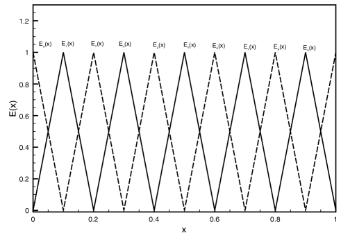
An illustrative example is given by the basis of functions drawn in Fig. 2. Each function $E^{(\alpha)}$ has a triangular shape centered in $x_{\alpha}$ and it vanishes outside the interval $(x_{\alpha-1},x_{\alpha+1})$. For any $y$, only two triangular functions are non zero and their sum is always equal to one.

With a general interpolation basis, PDFs at the initial scale can be approximated as

$$f_{k}(y,Q_{0}^{2})\equiv f^{0}_{k}(y)=\sum_{\alpha=1}^{N_{x}}f^{0}_{k}(x_{\alpha})\,\mathcal{I}^{(\alpha)}(y)+\mathcal{O}[(x_{\alpha+1}-x_{\alpha})^{p}]\,,$$ (16)

where $p$ is the lowest order neglected in the interpolation. With the (linear) triangular basis Fig. 2 $p=2$. Dropping for simplicity the dependence on $Q_{0}^{2}$ and $Q^{2}_{I}$, Eq. (14) becomes

$$f_{j}(x_{I},Q^{2}_{I})\,\equiv f_{j}(x_{I}) = \sum_{k=1}^{N_{\mathrm{pdf}}}\sum_{\alpha=1}^{N_{x}}\,f^{0}_{k}(x_{\alpha})\,\int_{x_{I}}^{1}\,{{dy}\over{y}}\,\Gamma_{jk}\left({{x_{I}}\over{y}}\right)\,\mathcal{I}^{(\alpha)}(y)+\mathcal{O}[(x_{\alpha+1}-x_{\alpha})^{p}]$$

$$f_{j}(x_{I}) = \sum_{k=1}^{N_{\mathrm{pdf}}}\sum_{\alpha=1}^{N_{x}}\hat{\sigma}^{Ij}_{\alpha k}\,f_{k}^{0}(x_{\alpha})+\mathcal{O}[(x_{\alpha+1}-x_{\alpha})^{p}],$$ (17)

where

$$\hat{\sigma}^{j}_{\alpha k}(x_{I},Q_{0}^{2},Q^{2}_{I})\equiv\hat{\sigma}^{Ij}_{\alpha k}=\,\int_{x_{I}}^{1}{{dy}\over{y}}\,\Gamma_{jk}\left({{x_{I}}\over{y}}\right)\,\mathcal{I}^{(\alpha)}(y).$$ (18)

In our notation $I$ specifies the data point, $\alpha$ runs over the points in the $x$–grid and $(j,k)$ run over the PDFs which evolve coupled to each other. Having precomputed the $\hat{\sigma}^{Ij}_{\alpha k}$ coefficients for each point $I$, the evaluation of the PDFs only requires $N_{x}$ evaluations of the PDFs at the initial scale, independent of the point at which the evolved PDFs are needed, thereby reducing the computational cost of evolution.

Figure 3: Set of interpolating Hermite cubic functions in the [0,1] interval.

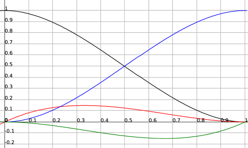
If the interpolation is performed on a more complicated set of functions than the triangular basis Fig. 2, better accuracy can be obtained with a smaller number of points and thus a reduced computational cost. For PDF evolution we will use the cubic Hermite interpolation drawn in Fig. 3. With this choice, for each interval $y\in[x_{\alpha},x_{\alpha+1})$ the function to be approximated can be written as

$$f^{0}_{k}(y) = h_{00}(t)f^{0}_{k}(x_{\alpha})+h_{10}(t)h_{\alpha}m_{\alpha}+h_{01}(t)f^{0}_{k}(x_{\alpha+1})+h_{11}(t)h_{\alpha}m_{\alpha+1}$$

$$+\mathcal{O}[(x_{\alpha+1}-x_{\alpha})^{4}],$$

where

$$h_{\alpha}=g(x_{{\alpha}+1})-g(x_{\alpha}),\qquad t={{g(y)-g(x_{\alpha})}\over{h_{\alpha}}},$$ (19)

and $g(y)$ is a monotonic function in [0,1] which determines the distribution of points in the interval (linear, logarithmic, etc.); $m_{\alpha}$ and $m_{\alpha+1}$ are derivatives of the interpolated function at the right and left–hand side of the interval, which can be defined as finite differences:

$$m_{\alpha}=\begin{cases}{{f^{0}_{k}(x_{\alpha})-f^{0}_{k}(x_{{\alpha}-1})}\over{2h_{\alpha-1}}}+{{f^{0}_{k}(x_{\alpha+1})-f^{0}_{k}(x_{\alpha})}\over{2h_{\alpha}}},&{\small\mbox{for }2\leq\alpha\leq N_{x}-1}\\ {{f^{0}_{k}(x_{\alpha+1})-f^{0}_{k}(x_{\alpha})}\over{h_{\alpha}}},&{\small\mbox{for }\alpha=1}\\ {{f^{0}_{k}(x_{\alpha})-f^{0}_{k}(x_{\alpha-1})}\over{h_{\alpha-1}}},&{\small\mbox{for }\alpha=N_{x}.}\end{cases}$$ (20)

Finally the functions $h$ are 3^rd–order polynomials drawn in Fig. 3 and defined as

$$h_{00}(t) = 2t^{3}-3t^{2}+1=(1+2t)(1-t)^{2}$$ (21)

$$h_{10}(t) = t^{3}-2t^{2}+t=t(t-1)^{2}$$

$$h_{01}(t) = -2t^{3}+3t^{2}=t^{2}(3-2t)$$

$$h_{11}(t) = t^{3}-t^{2}=t^{2}(t-1)$$

Collecting all terms, Eq. (3.1) becomes

$$f^{0}_{k}(y) = f^{0}_{k}(x_{\alpha-1})\,A^{(\alpha)}(y)+f^{0}_{k}(x_{\alpha})\,B^{(\alpha)}(y)+f^{0}_{k}(x_{\alpha+1})\,C^{(\alpha)}(y)$$

$$+f^{0}_{k}(x_{\alpha+2})\,D^{(\alpha)}(y)+\mathcal{O}[(x_{\alpha+1}-x_{\alpha})^{4}].$$

Hence the function, at any given point $y$ is obtained as a linear combination of $f^{0}$ at the four nearest points in the grid. The coefficients of such combination are given by:

$$A^{(\alpha)}(y) =\begin{cases}0,&\mbox{for }\alpha=1\\ -h_{10}(t){{h_{\alpha}}\over{h_{\alpha-1}}},&\mbox{for }\alpha\neq 1\end{cases}$$ (23)

$$B^{(\alpha)}(y) =\begin{cases}h_{00}(t)-h_{10}(t)-{{h_{11}(t)}\over{2}},&\mbox{for }\alpha=1\\ h_{00}(t)-{{h_{10}(t)}\over{2}}\left(1-{{h_{\alpha}}\over{h_{\alpha+1}}}\right)-h_{11}(t),&\mbox{for }\alpha=N_{x}-1\\ h_{00}(t)-{{h_{10}(t)}\over{2}}\left(1-{{h_{\alpha}}\over{h_{\alpha+1}}}\right)-{{h_{11}(t)}\over{2}},&\mbox{for }\alpha\neq 1,N_{x}-1\end{cases}$$

$$C^{(\alpha)}(y) =\begin{cases}h_{01}(t)+{{h_{11}(t)}\over{2}}\left(1-{{h_{\alpha}}\over{h_{\alpha+1}}}\right)+h_{10}(t),&\mbox{for }\alpha=1\\ h_{01}(t)+h_{11}(t)+{{h_{10}(t)}\over{2}},&\mbox{for }\alpha=N_{x}-1\\ h_{01}(t)+{{h_{11}(t)}\over{2}}\left(1-{{h_{\alpha}}\over{h_{\alpha+1}}}\right)+{{h_{10}(t)}\over{2}},&\mbox{for }\alpha\neq 1,N_{x}-1\end{cases}$$

$$D^{(\alpha)}(y) =\begin{cases}0,&\mbox{for }\alpha=N_{x}-1\\ h_{11}(t){{h_{\alpha}}\over{2h_{\alpha+1}}},&\mbox{for }\alpha\neq N_{x}-1\end{cases}$$

If we substitute Eq. (3.1) into the integral for the evolution of the PDFs, with $\xi$ the index such that

$$x_{\xi}\leq x_{I}<x_{\xi+1},$$

we end up with the following expressions for the $\hat{\sigma}$ coefficients

$$\hat{\sigma}^{Ij}_{\alpha k}=\begin{cases}\int_{x_{I}}^{x_{\xi+1}}\,{{dy}\over{y}}\,\Gamma_{jk}\left({{x_{I}}\over{y}}\right)\,A^{(\xi)}(y),&\mbox{for~{}}\alpha=\xi,\\ \int_{x_{I}}^{x_{\xi+1}}\,{{dy}\over{y}}\,\Gamma_{jk}\left({{x_{I}}\over{y}}\right)\,B^{(\xi)}(y)&\\ \quad+\theta(N_{x}-(\xi+2))\int_{x_{\xi+1}}^{x_{\xi+2}}\,{{dy}\over{y}}\,\Gamma_{jk}\left({{x_{I}}\over{y}}\right)\,A^{(\xi+1)}(y),&\mbox{for~{}}\alpha=\xi+1,\\ \int_{x_{I}}^{x_{\xi+1}}\,{{dy}\over{y}}\,\Gamma_{jk}\left({{x_{I}}\over{y}}\right)\,C^{(\xi)}(y)&\\ \quad+\theta(N_{x}-(\xi+2))\int_{x_{\xi+1}}^{x_{\xi+2}}\,{{dy}\over{y}}\,\Gamma_{jk}\left({{x_{I}}\over{y}}\right)\,B^{(\xi+1)}(y)&\\ \quad+\theta(N_{x}-(\xi+3))\int_{x_{\xi+2}}^{x_{\xi+3}}\,{{dy}\over{y}}\,\Gamma_{jk}\left({{x_{I}}\over{y}}\right)\,A^{(\xi+2)}(y),&\mbox{for~{}}\alpha=\xi+2,\\ \theta(N_{x}-(I-1))\int_{x_{\alpha-2}}^{x_{\alpha-1}}\,{{dy}\over{y}}\,\Gamma_{jk}\left({{x_{I}}\over{y}}\right)\,D^{(\alpha-1)}(y)&\\ \quad+\theta(N_{x}-\alpha)\int_{x_{\alpha-1}}^{x_{\alpha}}\,{{dy}\over{y}}\,\Gamma_{jk}\left({{x_{I}}\over{y}}\right)\,C^{(\alpha-1)}(y)&\\ \quad+\theta(N_{x}-(\alpha+1))\int_{x_{\alpha}}^{x_{\alpha+1}}\,{{dy}\over{y}}\,\Gamma_{jk}\left({{x_{I}}\over{y}}\right)\,B^{(\alpha)}(y)&\\ \quad+\theta(N_{x}-(\alpha+2))\int_{x_{\alpha+1}}^{x_{\alpha+2}}\,{{dy}\over{y}}\,\Gamma_{jk}\left({{x_{I}}\over{y}}\right)\,A^{(\alpha+1)}(y),&\mbox{for~{}}\xi+3\leq\alpha\leq N_{x}+1,\\ 0&\mbox{for~{}}\alpha<\xi.\\ \end{cases}$$ (24)

Despite the complicated bookkeeping, these expressions can be easily pre–computed and input into the fit.

A final remark: because of the divergent behaviour of the $x$–space evolution kernel at $x=1$, the integrals including $x_{I}$ in the integration interval need to be regularized in $y\sim x_{I}$. If we consider for instance the first integral of $A^{(\alpha)}$ in Eqn.(24), we can perform the same subtraction as in Ref. [4] in order to have a consistent definition of all precomputed coefficients:

$$\int_{x_{I}}^{x_{\xi+1}}{{dy}\over{y}}\,\Gamma_{jk}\left({{x_{I}}\over{y}}\right)\,A^{(\xi)}(y)$$

$$\qquad=\mbox{$\int_{x_{I}}^{x_{\xi+1}}{{dy}\over{y}}\,\Gamma_{jk}\left({{x_{I}}\over{y}}\right)\,\left(A^{(\xi)}(y)\,-\,{{x_{I}}\over{y}}A^{(\xi)}(x_{I})\right)+\,A^{(\xi)}(x_{I})\,\int_{x_{I}}^{x_{\xi+1}}{{dy}\over{y^{2}}}\,\Gamma_{jk}\left({{x_{I}}\over{y}}\right)$}$$

$$\qquad=\mbox{$\int_{x_{I}}^{x_{\xi+1}}{{dy}\over{y}}\,\Gamma_{jk}\left({{x_{I}}\over{y}}\right)\,\left(A^{(\xi)}(y)-\,{{x_{I}}\over{y}}A^{(\xi)}(x_{I})\right)+\,A^{(\xi)}(x_{I})\,\int_{x_{I}/x_{\xi+1}}^{1}dz\,\Gamma_{jk}(z)$}$$

$$\qquad=\mbox{$\int_{x_{I}}^{x_{\xi+1}}{{dy}\over{y}}\,\Gamma_{jk}\left({{x_{I}}\over{y}}\right)\,\left(A^{(\xi)}(y)-\,{{x_{I}}\over{y}}A^{(\xi)}(x_{I})\right)$}$$

$$\qquad\qquad\qquad\qquad+\mbox{$\,A^{(\xi)}(x_{I})\,\big{[}\Gamma_{jk}(N)\big{|}_{N=2}-\int_{0}^{x_{I}/x_{\xi+1}}dz\,\Gamma_{jk}(z)\big{]}$}.$$ (25)

As a result all $\hat{\sigma}$ are regularized; they can be stored once and for all for each experimental point, given that they do not depend on the PDF at the initial scale.

Figure 4: The sampling grid of $x$ values used for evolution superposed to the Les Houches gluon and 25 replicas of the gluon distribution from the NNPDF2.0 set at the starting scale.

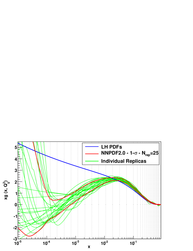
The accuracy of our PDF evolution code, described above, has been cross–checked against the Les Houches PDF evolution benchmark tables, originally produced from the comparison of the HOPPET [51] and PEGASUS [53] codes. In order to perform a meaningful comparison, we use the same settings described in detail in Ref. [15]. We show in Table 5 the relative difference for various combinations of PDFs between our PDF evolution and the benchmark tables of Ref. [15] at NLO in the ZM–VFNS, for three different grids. In each grid, the interval $[x_{\mathrm{min}},1]$ is divided into a log region at small $x$ and a linear region medium–high $x$. As we can see, the choice of a relatively small grid of 50 points leads to reproducing the Les Houches tables with an accuracy of $\mathcal{O}(10^{-5})$, more than enough for the precision phenomenology we aim to. Note that even though of course each individual replica has more structure than the average PDF, and much more structure than the simple Les Houches toy PDFs, they are still quite smooth on the scale of this grid, as it can be seen in Fig. 4. This ensures that benchmarking with the Les Houches table is adequate to guarantee the accuracy of our evolution code.

x (30 pts)	$e_{\mathrm{rel}}(u_{v})$	$e_{\mathrm{rel}}(d_{v})$	$e_{\mathrm{rel}}(\Sigma)$	$e_{\mathrm{rel}}(g)$
$1\cdot 10^{-7}$	$2.5\cdot 10^{-4}$	$3.5\cdot 10^{-4}$	$2.1\cdot 10^{-4}$	$2.1\cdot 10^{-4}$
$1\cdot 10^{-6}$	$1.6\cdot 10^{-3}$	$1.5\cdot 10^{-3}$	$2.3\cdot 10^{-4}$	$2.5\cdot 10^{-4}$
$1\cdot 10^{-5}$	$1.5\cdot 10^{-3}$	$1.4\cdot 10^{-3}$	$2.5\cdot 10^{-4}$	$2.8\cdot 10^{-4}$
$1\cdot 10^{-4}$	$6.5\cdot 10^{-4}$	$5.1\cdot 10^{-4}$	$3.0\cdot 10^{-4}$	$3.4\cdot 10^{-4}$
$1\cdot 10^{-3}$	$6.5\cdot 10^{-4}$	$4.7\cdot 10^{-4}$	$3.4\cdot 10^{-4}$	$3.9\cdot 10^{-4}$
$1\cdot 10^{-2}$	$1.4\cdot 10^{-3}$	$1.9\cdot 10^{-3}$	$3.4\cdot 10^{-4}$	$5.3\cdot 10^{-4}$
$1\cdot 10^{-1}$	$7.0\cdot 10^{-4}$	$1.0\cdot 10^{-3}$	$1.1\cdot 10^{-4}$	$4.1\cdot 10^{-4}$
$3\cdot 10^{-1}$	$1.9\cdot 10^{-5}$	$8.6\cdot 10^{-5}$	$1.3\cdot 10^{-5}$	$5.8\cdot 10^{-5}$
$5\cdot 10^{-1}$	$1.5\cdot 10^{-4}$	$1.8\cdot 10^{-4}$	$1.0\cdot 10^{-4}$	$1.1\cdot 10^{-4}$
$7\cdot 10^{-1}$	$3.8\cdot 10^{-4}$	$3.9\cdot 10^{-5}$	$3.1\cdot 10^{-4}$	$2.8\cdot 10^{-4}$
$9\cdot 10^{-1}$	$8.5\cdot 10^{-3}$	$9.5\cdot 10^{-2}$	$3.4\cdot 10^{-3}$	$2.0\cdot 10^{-2}$

x (50 pts)	$e_{\mathrm{rel}}(u_{v})$	$e_{\mathrm{rel}}(d_{v})$	$e_{\mathrm{rel}}(\Sigma)$	$e_{\mathrm{rel}}(g)$
$1\cdot 10^{-7}$	$2.1\cdot 10^{-4}$	$2.3\cdot 10^{-4}$	$2.7\cdot 10^{-5}$	$4.7\cdot 10^{-6}$
$1\cdot 10^{-6}$	$8.9\cdot 10^{-5}$	$8.4\cdot 10^{-5}$	$3.0\cdot 10^{-5}$	$2.1\cdot 10^{-5}$
$1\cdot 10^{-5}$	$9.3\cdot 10^{-5}$	$6.0\cdot 10^{-5}$	$2.3\cdot 10^{-5}$	$2.0\cdot 10^{-5}$
$1\cdot 10^{-4}$	$4.5\cdot 10^{-5}$	$2.8\cdot 10^{-5}$	$4.4\cdot 10^{-5}$	$4.2\cdot 10^{-5}$
$1\cdot 10^{-3}$	$3.0\cdot 10^{-5}$	$1.7\cdot 10^{-5}$	$4.0\cdot 10^{-5}$	$3.5\cdot 10^{-5}$
$1\cdot 10^{-2}$	$7.9\cdot 10^{-5}$	$6.8\cdot 10^{-5}$	$4.5\cdot 10^{-5}$	$5.8\cdot 10^{-5}$
$1\cdot 10^{-1}$	$1.7\cdot 10^{-4}$	$2.1\cdot 10^{-4}$	$1.6\cdot 10^{-5}$	$3.9\cdot 10^{-5}$
$3\cdot 10^{-1}$	$9.1\cdot 10^{-6}$	$3.9\cdot 10^{-5}$	$1.1\cdot 10^{-5}$	$1.9\cdot 10^{-7}$
$5\cdot 10^{-1}$	$2.4\cdot 10^{-5}$	$2.2\cdot 10^{-5}$	$2.2\cdot 10^{-5}$	$2.2\cdot 10^{-5}$
$7\cdot 10^{-1}$	$9.1\cdot 10^{-5}$	$1.5\cdot 10^{-5}$	$7.8\cdot 10^{-5}$	$1.2\cdot 10^{-4}$
$9\cdot 10^{-1}$	$1.0\cdot 10^{-3}$	$3.3\cdot 10^{-3}$	$8.0\cdot 10^{-4}$	$2.8\cdot 10^{-3}$

x (100 pts)	$e_{\mathrm{rel}}(u_{v})$	$e_{\mathrm{rel}}(d_{v})$	$e_{\mathrm{rel}}(\Sigma)$	$e_{\mathrm{rel}}(g)$
$1\cdot 10^{-7}$	$3.2\cdot 10^{-5}$	$5.0\cdot 10^{-5}$	$5.4\cdot 10^{-6}$	$2.0\cdot 10^{-5}$
$1\cdot 10^{-6}$	$2.6\cdot 10^{-6}$	$1.3\cdot 10^{-6}$	$5.7\cdot 10^{-6}$	$5.9\cdot 10^{-6}$
$1\cdot 10^{-5}$	$1.1\cdot 10^{-5}$	$2.2\cdot 10^{-5}$	$3.7\cdot 10^{-6}$	$1.0\cdot 10^{-5}$
$1\cdot 10^{-4}$	$1.8\cdot 10^{-5}$	$3.3\cdot 10^{-6}$	$1.3\cdot 10^{-5}$	$6.9\cdot 10^{-6}$
$1\cdot 10^{-3}$	$1.3\cdot 10^{-6}$	$4.9\cdot 10^{-6}$	$4.7\cdot 10^{-6}$	$7.7\cdot 10^{-6}$
$1\cdot 10^{-2}$	$1.6\cdot 10^{-5}$	$1.7\cdot 10^{-5}$	$4.8\cdot 10^{-6}$	$1.1\cdot 10^{-6}$
$1\cdot 10^{-1}$	$3.4\cdot 10^{-5}$	$2.9\cdot 10^{-5}$	$8.7\cdot 10^{-6}$	$2.1\cdot 10^{-6}$
$3\cdot 10^{-1}$	$2.0\cdot 10^{-6}$	$2.5\cdot 10^{-5}$	$7.9\cdot 10^{-6}$	$3.9\cdot 10^{-6}$
$5\cdot 10^{-1}$	$1.7\cdot 10^{-5}$	$1.3\cdot 10^{-5}$	$1.7\cdot 10^{-5}$	$3.1\cdot 10^{-5}$
$7\cdot 10^{-1}$	$7.1\cdot 10^{-5}$	$8.3\cdot 10^{-6}$	$6.3\cdot 10^{-5}$	$1.3\cdot 10^{-4}$
$9\cdot 10^{-1}$	$3.9\cdot 10^{-5}$	$3.8\cdot 10^{-4}$	$2.5\cdot 10^{-5}$	$1.7\cdot 10^{-3}$

Table 5: Relative accuracy of FastKernel evolution compared to the Les Houches benchmark tables for PDFs evolved to the scale $Q^{2}=10^{4}$ GeV². The interpolation is performed on cubic Hermite polynomials and the grid is composed of 30 points (top), 50 points (middle), or 100 points (bottom), distributed logarithmically in the small–$x$ region and linearly in the medium– and large–$x$ region.

3.2 Fast computation of DIS observables

Using the strategy described in the previous section, we can easily write down the expression for the DIS observables included in our fit and show explicitly how their computation works on the interpolation basis. The basic idea [3, 4] is that, starting with the standard factorized expression

$$\sigma_{I}^{DIS}(x_{I},Q^{2}_{I})=\sum_{k=1}^{N_{\mathrm{pdf}}}C_{Ik}\otimes f_{k}(x_{I},Q^{2}_{I})\equiv\sum_{k=1}^{N_{\mathrm{pdf}}}\,\int_{x_{I}}^{1}\,{{dy}\over{y}}\,C_{Ik}\left({{x_{I}}\over{y}},\alpha_{s}(Q^{2}_{I})\right)\,f_{k}(y,Q^{2}_{I}).$$ (26)

(where $I$ denotes both the observable and the kinematic point), we can absorb the coefficient function $C_{Ik}$ into a modified evolution kernel $K_{Ij}$ which can be precomputed before starting the fit (see Appendix A of Ref. [4]):

$$K_{Ij}(x_{I},\alpha_{s}(Q_{I}^{2}),\alpha_{s}(Q_{0}^{2}))=\sum_{k=1}^{N_{\mathrm{pdf}}}C_{Ik}\otimes\Gamma_{kj}(x_{I},\alpha_{s}(Q_{I}^{2}),\alpha_{s}(Q_{0}^{2})).$$ (27)

The kernel acts on the $j$–th PDFs at the initial scale, and it is an observable–dependent linear combination of products of coefficient functions and evolution kernels:

$$\sigma_{I}^{DIS}(x_{I},Q^{2}_{I})=\sum_{j=1}^{N_{\mathrm{pdf}}}\,K_{Ij}\otimes f_{j}^{0}\equiv\sum_{j=1}^{N_{\mathrm{pdf}}}\,\int_{x_{I}}^{1}\,{{dy}\over{y}}\,c_{k}\,K_{Ij}\left({{x_{I}}\over{y}},\alpha_{s}(Q_{I}^{2}),\alpha_{s}(Q_{0}^{2})\right)f^{0}_{j}(y,Q_{0}^{2}).$$ (28)

If we substitute Eq. (17) into the expression for the observable, we can write it as:

$$\sigma_{I}^{DIS}(x_{I},Q^{2}_{I}) = \sum_{j=1}^{N_{\mathrm{pdf}}}\sum_{\alpha=1}^{N_{x}}\,f_{j}^{0}(x_{\alpha})\,\int_{x_{I}}^{1}\,{{dy}\over{y}}\,K_{Ij}\left({{x_{I}}\over{y}}\right)\,\mathcal{I}^{(\alpha)}(y)$$

$$= \sum_{j=1}^{N_{\mathrm{pdf}}}\sum_{\alpha=1}^{N_{x}}f^{0}_{j}(x_{\alpha})\,\hat{\sigma}^{I}_{\alpha j}+\mathcal{O}[(x_{\alpha+1}-x_{\alpha})^{p}],$$

where

$$\hat{\sigma}^{I}_{\alpha j}(x_{I},Q_{0}^{2},Q_{I}^{2})\equiv\hat{\sigma}^{I}_{\alpha j}=\,\int_{x_{I}}^{1}{{dy}\over{y}}\,K_{Ij}\left({{x_{I}}\over{y}},\alpha_{s}(Q_{I}^{2}),\alpha_{s}(Q_{0}^{2})\right)\,\mathcal{I}^{(\alpha)}(y).$$ (30)

Now the only index running over the PDF basis is $j$ because the other index $k$ is contracted in the definition of $K$.

Consider for example the expression for the deuteron structure function. We can write down explicitly the terms of Eq. (3.2) as:

$$F_{2}^{d}(x_{I},Q_{I}^{2})=\sum_{\alpha=1}^{N_{x}}\,\sigma_{\alpha 10}^{I}\,f_{10}(x_{\alpha})+\sigma_{\alpha 1}^{I}\,f_{1}(x_{\alpha})+\sigma_{\alpha 2}^{I}\,f_{2}(x_{\alpha})+\mathcal{O}[(x_{\alpha+1}-x_{\alpha})^{p}],$$ (31)

with

$$\sigma_{\alpha 10} = \int_{x_{I}}^{1}\,{{dy}\over{y}}\,{{1}\over{18}}\left(C_{2,q}\otimes\Gamma^{-}\right)\left({{x_{I}}\over{y}}\right)\,\mathcal{I}^{(\alpha)}(y)$$

$$\sigma_{\alpha 1} = \int_{x_{I}}^{1}\,{{dy}\over{y}}\,\big{[}-{{1}\over{18}}\left(C_{2,q}\otimes\Gamma^{15,q}\right)\left({{x_{I}}\over{y}}\right)+{{1}\over{30}}\left(C_{2,q}\otimes\Gamma^{24,q}\right)\left({{x_{I}}\over{y}}\right)$$

$$-{{1}\over{30}}\left(C_{2,q}\otimes\Gamma^{35,q}\right)\left({{x_{I}}\over{y}}\right)+{{5}\over{18}}\left(C_{2,q}\otimes\Gamma^{S,qq}\right)\left({{x_{I}}\over{y}}\right)$$

$$-c_{g}(n_{f})\left(C_{2,g}\otimes\Gamma^{S,gq}\right)\left({{x_{I}}\over{y}}\right)\big{]}\mathcal{I}^{(\alpha)}(y)$$

$$\sigma_{\alpha 2} = \int_{x_{I}}^{1}\,{{dy}\over{y}}\,\big{[}-{{1}\over{18}}\left(C_{2,q}\otimes\Gamma^{15,q}\right)\left({{x_{I}}\over{y}}\right)+{{1}\over{30}}\left(C_{2,q}\otimes\Gamma^{24,g}\right)\left({{x_{I}}\over{y}}\right)$$ (32)

$$\hskip 8.5359pt-\mbox{${{1}\over{30}}\left(C_{2,q}\otimes\Gamma^{35,g}\right)\left({{x_{I}}\over{y}}\right)+{{5}\over{18}}\left(C_{2,q}\otimes\Gamma^{S,qg}\right)\left({{x_{I}}\over{y}}\right)$}$$

$$\hskip 8.5359pt-\mbox{$c_{g}(n_{f})\left(C_{2,g}\otimes\Gamma^{S,gg}\right)\left({{x_{I}}\over{y}}\right)\big{]}\mathcal{I}^{(\alpha)}(y)$}$$

where all kernels and coefficient functions are defined in Ref. [4] and

$$f^{0}_{10}=T_{8,0}\qquad f^{0}_{1}=\Sigma_{0}\qquad f^{0}_{2}=g_{0}$$

in the evolution basis of Eq. (13).

3.3 Fast computation of hadronic observables

The FastKernel implementation of hadronic observables requires a double convolution of the coefficient function with two parton distributions. We could follow the same strategy used for DIS: construct a kernel for each observable and each pair of initial PDFs, and then compute the double convolution with a suitable generalization of the method introduced in Sect. 3.2. However, for hadronic observables, we adopt a somewhat different strategy, which allows us to treat in a more symmetric way processes for which a fast interface already exists (such as jets) and those (such as DY) for which we have to develop our own interface. Namely, instead of including the coefficient function into the kernel according to Eq. (27), we compute the convolution Eq. (26) using the fast interpolation method.

To see how this works, consider first the case of a process with only one parton in the initial state. Starting from Eq. (26), we can project the evolved PDF $f_{k}$ onto an interpolation basis as follows:

$$\sigma_{I}^{DIS}(x_{I},Q^{2}_{I})=\sum_{k=1}^{N_{\mathrm{pdf}}}\sum_{\alpha=1}^{N_{y}}\,f_{k}(y_{\alpha},Q^{2}_{I})\int_{x_{I}}^{1}\,{{dy}\over{y}}\,C_{Ik}\left({{x_{I}}\over{y}},\alpha_{s}(Q^{2}_{I})\right)\,\mathcal{I}^{\alpha}(y)+\mathcal{O}[(y_{\alpha+1}-y_{\alpha})^{q}],$$ (33)

where $q$ indicates the first order neglected in the interpolation of the evolved PDFs. This defines another grid of points, $\{y_{\alpha}\}$, upon which the coefficients can be pre–computed before starting the fit:

$$\int_{x_{I}}^{1}\,{{dy}\over{y}}\,C_{Ik}\left({{x_{I}}\over{y}},\alpha_{s}(Q^{2}_{I})\right)\,\mathcal{I}^{\alpha}(y)\equiv C_{Ik}^{\alpha}.$$ (34)

If, on top of this interpolation, we interpolate the parton distributions at the initial scale on the $\{x_{\alpha}\}$ grid as we did in the previous subsection, we get

$$\sigma_{I}^{DIS}(x_{I},Q^{2}_{I}) = \sum_{k=1}^{N_{\mathrm{pdf}}}\,\sum_{\alpha=1}^{N_{y}}f_{k}(y_{\alpha},Q^{2}_{I})\,C_{Ik}^{\alpha}+\mathcal{O}[(y_{\alpha+1}-y_{\alpha})^{q}]$$

$$= \sum_{k,n=1}^{N_{\mathrm{pdf}}}\sum_{\alpha=1}^{N_{y}}\sum_{\beta=1}^{N_{x}}\,C_{Ik}^{\alpha}\,\hat{\sigma}^{\alpha,I}_{\beta kn}\,f^{0}_{n}(x_{\beta})+\mathcal{O}[(y_{\alpha+1}-y_{\alpha})^{q}(x_{\beta+1}-x_{\beta})^{p}].$$

Notice that the two interpolations are independent of each other. The number of points $N_{x}$ and $N_{y}$ in each grid, the interpolating functions, and the interpolation orders $p$ and $q$ are not necessarily the same.

We now apply this to the rapidity–differential Drell–Yan cross section, introduced in Sect. 2.2, to exemplify the procedure. The NLO cross section is given by

$${{d\sigma^{\mathrm{DY}}}\over{dQ_{I}^{2}dY_{I}}} = n(Q_{I}^{2})\sum_{j=1}^{N_{q}}e_{j}^{2}\,\int_{x^{0}_{1}}^{1}\,dx_{1}\,\int_{x^{0}_{2}}^{1}\,dx_{2}$$

$$\,\,\bigg{\{}\left[q_{j}(x_{1},Q_{I}^{2})\bar{q}_{j}(x_{2},Q_{I}^{2})+q_{j}(x_{2},Q_{I}^{2})\bar{q}_{j}(x_{1},Q_{I}^{2})\right]\,\left(D^{\mathrm{qq}}(x_{1},x_{2},Y_{I})\right)$$

$$\hskip 56.9055pt+g(x_{1},Q_{I}^{2})\left[q_{j}(x_{2},Q_{I}^{2})+\bar{q}_{j}(x_{2},Q_{I}^{2})\right]\,\left(D^{\mathrm{gq}}(x_{1},x_{2},Y_{I})\right)$$

$$\hskip 56.9055pt+g(x_{2},Q_{I}^{2})\left[q_{j}(x_{1},Q_{I}^{2})+\bar{q}_{j}(x_{1},Q_{I}^{2})\right]\,\left(D^{\mathrm{qg}}(x_{1},x_{2},Y_{I})\right)\bigg{\}},$$

where the normalization factor is explicitly written in Sect. 2.2 and the coefficient functions can be found in Refs. [54, 55] (see also Appendix B).

For each point of the interpolation grid, we define a set of two–dimensional interpolating functions as the product of one–dimensional functions defined in Eq. (15):

$$\mathcal{I}^{(\alpha,\beta)}(x_{1},x_{2})\,\equiv\,\mathcal{I}^{(\alpha)}(x_{1})\mathcal{I}^{(\beta)}(x_{2}).$$ (37)

The product of two functions can be approximated by means of these interpolating functions as

$$f(y_{1})h(y_{2})=\sum_{\alpha,\beta=1}^{N_{y}}f(y_{1,\alpha})h(y_{2,\beta})\,\mathcal{I}^{(\alpha,\beta)}(y_{1},y_{2})+\mathcal{O}[(y_{1,\alpha+1}-y_{1,\alpha})^{q}(y_{2,\beta+1}-y_{2,\beta})^{q}].$$ (38)

Applying Eq. (38) to the PDFs in Eq. (3.3), we get

$${{d\sigma^{\mathrm{DY}}}\over{dQ_{I}^{2}dY_{I}}} = n(Q_{I}^{2})\sum_{j=1}^{N_{q}}e_{j}^{2}\sum_{\alpha,\beta=1}^{N_{x}}\,\big{[}q_{j}(y_{1,\alpha})\bar{q}_{j}(y_{2,\beta})+\bar{q}_{j}(y_{1,\alpha})q_{j}(y_{2,\beta})\big{]}$$

$$\hskip 36.98866pt\int_{x^{0}_{1}}^{1}\,dx_{1}\,\int_{x^{0}_{2}}^{1}\,dx_{2}\mathcal{I}^{(\alpha,\beta)}(x_{1},x_{2})\,D^{\mathrm{qq}}(x_{1},x_{2},Y_{I})$$

$$+\big{[}g(y_{1,\alpha})(q_{j}(y_{2,\beta})+\bar{q}_{j}(y_{2,\beta}))\big{]}\int_{x^{0}_{1}}^{1}\,dx_{1}\,\int_{x^{0}_{2}}^{1}\,dx_{2}\mathcal{I}^{(\alpha,\beta)}(x_{1},x_{2})\,D^{\mathrm{gq}}(x_{2},x_{1},Y_{I})$$

$$+\big{[}g(y_{1,\alpha})(q_{j}(y_{2,\beta})+\bar{q}_{j}(y_{2,\beta}))\big{]}\int_{x^{0}_{1}}^{1}\,dx_{1}\,\int_{x^{0}_{2}}^{1}\,dx_{2}\mathcal{I}^{(\alpha,\beta)}(x_{1},x_{2})\,D^{\mathrm{gq}}(x_{1},x_{2},Y_{I})$$

$$\hskip 85.35826pt+\mathcal{O}[(y_{1,\alpha+1}-y_{1,\alpha})^{q}(y_{2,\beta+1}-y_{2,\beta})^{q}],$$

where at next–to–leading order $D^{\mathrm{qg}}(x_{1},x_{2},Y_{I})=D^{\mathrm{gq}}(x_{2},x_{1},Y_{I})$. Therefore, we can define

$$C_{I,ij}^{(\alpha,\beta)}\equiv\int_{x^{0}_{1}}^{1}dx_{1}\,\int_{x^{0}_{2}}^{1}dx_{2}\mathcal{I}^{(\alpha,\beta)}(x_{1},x_{2})\,D^{\mathrm{ij}}(x_{1},x_{2},Y_{I}),$$ (40)

where $i,j$ run over the non–zero combinations of $q,\bar{q}$ and $g$. By substituting them into Eq. (3.3), we end up with the expression

$${{d\sigma^{\mathrm{DY}}}\over{dQ_{I}^{2}dY_{I}}} = n(Q_{I}^{2})\sum_{j=1}^{N_{q}}e_{j}^{2}\,\sum_{\alpha,\beta=1}^{N_{y}}C_{I,qq}^{(\alpha,\beta)}\left[q_{j}(y_{1,\alpha})\bar{q}_{j}(y_{2,\beta})+\bar{q}_{j}(y_{1,\alpha})q_{j}(y_{2,\beta})\right]$$ (41)

$$\hskip 28.45274pt+C_{I,gq}^{(\alpha,\beta)}\left[g(y_{1,\alpha})(q_{j}(y_{2,\beta})+\bar{q}_{j}(y_{2,\beta}))\right]$$

$$\hskip 28.45274pt+C_{I,qg}^{(\alpha,\beta)}\left[(q_{j}(y_{1,\alpha})+\bar{q}_{j}(y_{1,\alpha}))g(y_{2,\beta})\right]$$

$$\hskip 28.45274pt+\mathcal{O}[(y_{1,\alpha+1}-y_{1,\alpha})^{q}(y_{2,\beta+1}-y_{2,\beta})^{q}]\,,$$

which is the analogue of Eq. (33) for a hadronic observable. The physical basis $\{q\}_{j}$ and the evolution basis $\{f\}_{j}$ are related by a matrix $A$:

$$q_{j}=A_{jr}f_{r}\qquad\bar{q}_{j}=\bar{A}_{js}f_{s}\,.$$

Each PDF $f$ is evolved at the physical scale of the process, and the evolution matrix $\Gamma$ which relates the initial scale PDFs to the evolved ones is

$$f_{r}(x,Q^{2})=\Gamma_{rn}(x,Q_{0}^{2},Q^{2})\otimes f_{n}(x,Q_{0}^{2}).$$

Therefore Eq. (41) becomes

$${{d\sigma^{\mathrm{DY}}}\over{dQ_{I}^{2}dY_{I}}} = n(Q_{I}^{2})\sum_{j=1}^{N_{q}}e_{j}^{2}\,\sum_{\alpha,\beta=1}^{N_{y}}\sum_{r,s=1}^{N_{\mathrm{pdf}}}C_{I,qq}^{(\alpha,\beta)}(A_{jr}\bar{A}_{js}+\bar{A}_{jr}A_{js})\,f_{r}(y_{1,\alpha})f_{s}(y_{2,\beta})$$

$$\hskip 28.45274pt+\left[C_{I,gq}^{(\alpha,\beta)}\delta_{r2}(A_{js}+\bar{A}_{js})+C_{I,qg}^{(\alpha,\beta)}(A_{jr}+\bar{A}_{js})\delta_{q2}\right]\,f_{r}(y_{1,\alpha})f_{s}(y_{2,\beta)})$$

$$\hskip 28.45274pt+\mathcal{O}[(y_{1,\alpha+1}-y_{1,\alpha})^{q}(y_{2,\beta+1}-y_{2,\beta})^{q}].$$

Defining

$$c_{rs} \equiv \sum_{j=1}^{N_{q}}e_{j}^{2}(A_{jr}\bar{A}_{js}+\bar{A}_{jr}A_{js})$$ (43)

$$d_{rs} \equiv \sum_{j=1}^{N_{q}}e_{j}^{2}\left[\delta_{r2}(A_{js}+\bar{A}_{js})+(A_{jr}+\bar{A}_{jr})\delta_{s2}\right]$$

and applying Eq. (17) to the evolved PDFs, we end up with a result which is similar to Eq. (3.3):

$${{d\sigma^{\mathrm{DY}}}\over{dQ_{I}^{2}dY_{I}}} = n(Q_{I}^{2})\sum_{\gamma,\delta=1}^{N_{x}}\sum_{l,m=1}^{N_{\mathrm{pdf}}}\bigg{[}\sum_{\alpha,\beta=1}^{N_{y}}\sum_{r,s=1}^{N_{\mathrm{pdf}}}c_{rs}C_{I,qq}^{(\alpha,\beta)}\hat{\sigma}^{\alpha,I}_{\gamma rl}\hat{\sigma}^{\beta,I}_{\delta sm}$$

$$+[d_{rs}C_{I,gq}^{(\alpha,\beta)}+d_{sr}C_{I,qg}^{(\alpha,\beta)}]\hat{\sigma}^{\alpha,I}_{\gamma rl}\hat{\sigma}^{\beta,I}_{\delta sm}\bigg{]}f^{(0)}_{l}(x_{1,\gamma})f^{(0)}_{m}(x_{2,\delta})$$

$$+\mathcal{O}[(y_{1,\alpha+1}-y_{1,\alpha})^{q}(y_{2,\beta+1}-y_{2,\beta})^{q}(x_{1,\gamma+1}-x_{1,\gamma})^{p}(x_{2,\delta+1}-x_{2,\delta})^{p}].$$

In order to define the coefficients in Eq. (3.3), we have to make an explicit choice of an interpolating basis. For the interpolation of the evolved PDFs we use the triangular interpolating basis drawn in Fig. 2, defined as

$$E^{(\alpha)}(y)={{y-y_{\alpha-1}}\over{y_{\alpha}-y_{\alpha-1}}}\theta[(y_{\alpha}-y)(y-y_{\alpha-1})]+{{y_{\alpha+1}-y}\over{y_{\alpha+1}-y_{\alpha}}}\theta[(y_{\alpha}-y)(y-y_{\alpha+1})].$$ (45)

With this definition, we can project the PDFs on the triangular basis

$$q(y)=\sum_{\alpha=1}^{N_{x}}q(y_{\alpha})\,E^{(\alpha)}(y)+\mathcal{O}[(y_{\alpha+1}-y_{\alpha})^{2}]$$

and define

$$C_{K,ij}^{(\alpha,\beta)}=\int_{x^{0}_{1}}^{1}dx_{1}\int_{x^{0}_{2}}^{1}dx_{2}\,E^{(\alpha)}(x_{1})\,E^{(\beta)}(x_{2})D^{(K)}_{ij}(x_{1},x_{2}),$$ (46)

where $K$ indicates the perturbative order and $i,j$ run over the non–zero combinations of $q,\bar{q}$ and $g$. To be more explicit, defining the index $\xi$ and $\zeta$ in such a way that

$$x_{\xi}<x_{1}^{0}<x_{\xi+1}\qquad x_{\zeta}<x_{2}^{0}<x_{\zeta+1},$$ (47)

we can give the precise definition of the NLO coefficients:

$$C_{K,ij}^{(\alpha,\beta)}=\begin{cases}\int_{x^{0}_{1}}^{x_{\alpha+1}}dx_{1}\int_{x^{0}_{2}}^{x_{\beta+1}}dx_{2}\,E^{(\alpha)}(x_{1})\,E^{(\beta)}(x_{2})D^{(K)}_{ij}(x_{1},x_{2}),&\,\alpha=\xi,\xi+1,\,\beta=\zeta,\zeta+1\\ \int_{x^{0}_{1}}^{x_{\alpha+1}}dx_{1}\int_{x^{\beta-1}}^{x_{\beta+1}}dx_{2}\,E^{(\alpha)}(x_{1})\,E^{(\beta)}(x_{2})D^{(K)}_{ij}(x_{1},x_{2}),&\,\alpha\leq\xi+1,\,\beta\geq\zeta+2,\\ \int_{x_{\alpha-1}}^{x_{\alpha+1}}dx_{1}\int_{x^{0}_{2}}^{x_{\beta+1}}dx_{2}\,E^{(\alpha)}(x_{1})\,E^{(\beta)}(x_{2})D^{(K)}_{ij}(x_{1},x_{2}),&\,\alpha\geq\xi+2,\,\beta\leq\zeta+1,\\ \int_{x_{\alpha-1}}^{x_{\alpha+1}}dx_{1}\int_{x_{\beta-1}}^{x_{\beta+1}}dx_{2}\,E^{(\alpha)}(x_{1})\,E^{(\beta)}(x_{2})D^{(K)}_{ij}(x_{1},x_{2}),&\,\alpha\geq\xi+2,\,\beta\geq\zeta+2,\\ 0&\,\alpha\leq\xi-1,\,\beta\leq\zeta-1,\\ \end{cases}$$ (48)

while the expression for the LO is trivial, given that $D^{(0)}_{q\bar{q}}(x_{1},x_{2})=\delta(x_{1}-x^{0}_{1})\delta(x_{2}-x^{0}_{2})$.

The FastKernel method for hadronic observables is easily interfaced to other existing fast codes, such as FastNLO for inclusive jets [16], by simply using FastKernel for the interpolation at the initial scale and parton evolution, and exploiting the existing interface for the convolution of the evolved PDF with the appropriate coefficient functions. In the particular case of the inclusive jet measurements used in the present analysis, the analogs of the coefficients $C_{I,ij}^{(\alpha,\beta)}$ in Eq. (41) can be directly extracted from the FastNLO precomputed tables through its interface, although in such case the relevant PDF combinations are different than those of the DY process Eq. (41).

3.4 FastKernel benchmarking

It is straightforward to extend the FastKernel method described in the previous section to all fixed–target DY and collider vector boson production datasets described in Sect. 2.2, using the appropriate couplings and PDF combinations. More details on the computation of these observables can be found in Appendix B.

In order to assess the accuracy of the method, we have benchmarked the results obtained with our code to those produced by an independent code [56] which computes the exact NLO cross sections for all relevant Drell–Yan distributions. The comparison is performed by using a given set of input PDFs and evaluating the various cross–sections for all observables included in the fit in the kinematical points which correspond to the included data.

The benchmarking of the FastKernel code for the Drell–Yan process has been performed for the following observables, introduced in Sect. 2.2:

• Rapidity and $x_{F}$ distributions and asymmetries for fixed target Drell–Yan in pp and pCu collisions (E605 and E866 kinematics)

• The $W$ rapidity distribution and asymmetries at hadron colliders (Tevatron kinematics)

• The $Z$ rapidity distribution at hadron colliders (Tevatron kinematics)

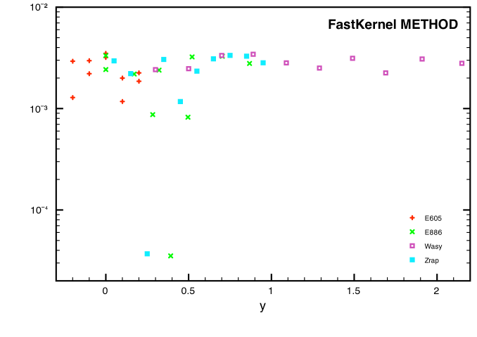
The results of this benchmark comparison are displayed in Fig. 5, where the relative accuracy between the FastKernel implementation and the exact code is shown for all data points included in the NNPDF2.0. This accuracy has been obtained with a grid of 100 points distributed as the root square of the log from $x_{\mathrm{min}}$ to 1.

It is clear from Fig. 5 that with a linear interpolation performed on a 100–points grid, we get a reasonable accuracy for all points, 1% in the worse case, which is suitable because the experimental uncertainties of the available datasets are rather larger (see Table 2). This accuracy can be improved arbitrarily by increasing the number of data points in the grid, with a very small cost in terms of speed: this is demonstrated in Fig. 6, where we show the improvement in accuracy obtained by using a grid of 500 points.

Figure 5: Relative accuracy for NLO Drell–Yan rapidity distributions using the FastKernel method, compared to the code of [56], as a function of rapidity $y$. Each point corresponds to the kinematics of a data point included in the NNPDF2.0 fit. The accuracy refers to a grid of 100 points distributed as the root square of the log from $x_{\mathrm{min}}$ to 1.

Figure 6: Same as Fig. 5, for 40 points in the kinematical range covered by the data points included in the NNPDF2.0 fit, using a grid of 500 points distributed as the root square of the log from $x_{\mathrm{min}}$ to 1.

4 Minimization and stopping

As discussed at length in Ref. [4], our parametrization of PDFs differs from other approaches in that we use an unbiased basis of functions characterized by a very large and redundant set of parameters: neural networks. This requires a detailed analysis of the fitting strategy. There are two difficulties that have to be overcome. First, it is necessary to devise an algorithm to fit neural network PDFs: observables depend nonlocally and sometimes nonlinearly on PDFs through convolutions, and the fitting strategy must deal with this dependence. We have solved this difficulty by means of genetic algorithms. Second, any redundant parameterization may accommodate not only the smooth shape of the “true” underlying PDFs, but also fluctuations of the experimental data. The best fit form of the set of PDFs is not just given by the absolute minimum of some figure of merit: it is the possibility of further decreasing the figure of merit which guarantees that the best fit is not driven by the functional form of the parameterization. The best fit is instead given by a suitable optimal training, beyond which the figure of merit improves only because one is fitting the statistical noise in the data, which raises the question of how this optimal fit is determined. We solve this through the so–called cross–validation method [57], based on the random separation of data into training and validation sets. Namely, PDFs are trained on a fraction of the data and validated on the rest of the data. Training is stopped when the quality of the fit to validation data deteriorates while the quality of the fit to training data keeps improving. This corresponds to the onset of a regime where neural networks start to fit random fluctuations rather than the underlying physics (overlearning).

4.1 Genetic algorithm strategy

The fitting of a set of neural networks (which parameterize the PDFs) to the data is performed by minimization of a suitably defined figure of merit [4]. This is a complex task for two reasons: we need to find a reasonable minimum in a very large parameter space, and the figure of merit to be minimized is a nonlocal functional of the set of functions which are being determined in the minimization. Genetic algorithms turn out to provide an efficient solution to this minimization problem.

The basic idea underlying genetic algorithm minimization is to create a pool of possible solutions to minimize the figure of merit, each one characterized by a set of parameters. Genetic algorithms work on the parameter space, creating new possible solutions and discarding those which are far from the minimum. As a consequence, the genetic algorithm cycle corresponds to successive generations where: i) we create new possible solutions by mutation and crossing; ii) we naturally select the best candidates and eliminate the rest. This strategy has proven to be generally very useful to deal with minimization of functional forms which are further convoluted to deliver observables (see Ref. [58, 59] for applications unrelated to PDF fitting).

The fitting of the neural networks on the individual replicas is performed by minimizing the error function [4]

$$E^{(k)}={{1}\over{N_{\mathrm{dat}}}}\sum_{I,J=1}^{N_{\rm dat}}\left(F_{I}^{(\mathrm{art})(k)}-F_{I}^{(\mathrm{net})(k)}\right)\left(\left({\mathrm{cov_{t_{0}}}}\right)^{-1}\right)_{IJ}\left(F_{J}^{(\mathrm{art})(k)}-F_{J}^{(\mathrm{net})(k)}\right)\ ,$$ (49)

where $F_{I}^{\rm(art)(k)}$ is the value of the observable $F_{I}$ at the kinematical point $I$ corresponding to the Monte Carlo replica $k$, and $F_{I}^{(\rm net)(k)}$ is the same observable computed from the neural network PDFs, and where the $t_{0}$ covariance matrix ${\rm cov_{t_{0}}}$ has been defined in Eq. (1). The details of how genetic algorithm minimization is applied to the problem of PDFs fitting was presented in Ref. [4]. This strategy has been now improved in order to deal with the addition of multiple new experimental datasets, as we shall now discuss.

4.2 Targeted weighted training

In order to deal more efficiently with the need of fitting data from a wide variety of different experiments and different datasets within an experiment we adopt a dynamical weighted fitting technique. The basic idea is to construct a minimization procedure that rapidly converges towards a configuration for which the final figure of merit $E^{(k)}$ is as even as possible among all the experimental sets. Weighted fitting consists of adjusting the weights of the datasets in the determination of the error function during the minimization procedure according to their individual figure of merit: datasets that yield a large contribution to the error function get a larger weight in the total figure of merit.

In a first epoch of the genetic algorithms minimization, weighted training is activated. This means than rather than Eq. (49), the actual function which is minimized is

$$E_{\rm wt}^{(k)}={{1}\over{N_{\mathrm{dat}}}}\sum_{j=1}^{N_{\mathrm{sets}}}p_{j}^{(k)}N_{\mathrm{dat},j}E_{j}^{(k)}\,,$$ (50)

where $E_{j}^{(k)}$ is the error function in Eq. (49) restricted to the dataset $j$, $N_{{\rm dat},j}$ is the number of points of this dataset and $p_{j}^{(k)}$ are weights associated to this dataset which are adjusted dynamically as described below.

In the present analysis, a different, more refined way of determining the weights $p_{j}^{(k)}$ has been adopted as compared to Refs. [3, 4]. The idea is the following: in the beginning of the fit, target values $E_{i}^{\rm targ}$ for the figure of merit of each experiment are chosen. Then, at each generation of the minimization, the weights of individual sets are updated using the conditions

1. If $E_{i}^{(k)}\geq E_{i}^{\rm targ}$, then $p_{i}^{(k)}=\left(E_{i}^{(k)}/E_{i}^{\rm targ}\right)^{2}$,

2. If $E_{i}^{(k)}<E_{i}^{\rm targ}$, then $p_{i}^{(k)}=0$  .

Hence, sets which are far above their target value will get a larger weight in the figure of merit. On the other hand, sets which are below their target are likely to be already learnt properly and thus are removed from the figure of merit which is being minimized. The determination of the target values $E_{i}^{\rm targ}$ for all the sets which enter into the fit is an iterative procedure that works as follows. We start with all $E_{i}^{\rm targ}=1$ and proceed to a first very long fit. Then, we use the outcome of the fit to produce a first nontrivial set of $E_{i}^{\rm targ}$ values. This procedure is iterated until convergence. In practice, convergence is very fast: we have used the values of $\left\langle E_{i}\right\rangle$ from a first batch of 100 replicas, in turn produced using as target values those of a previous very long fit; these values differ generally by $2-4$% (at most 10% in a couple cases) from the values of $\left\langle E_{i}\right\rangle$ for the reference fit shown in Table 10. This implementation of targeted weighted training is such that the error function of each dataset tends smoothly to its “natural” value, that is, $p_{i}^{(k)}\to 1$ as the minimization progresses. Those sets which are harder to fit are given more weight than the experiments that are learnt faster.

An important feature of weighted training is that weights are given to individual datasets (as identified in Table 1) and not just to experiments. This is motivated by the fact that typically each dataset covers a distinct, restricted kinematic region. Hence, the weighting takes care of the fact that the data in different kinematic regions carry different amounts of information and thus require unequal amounts of training.

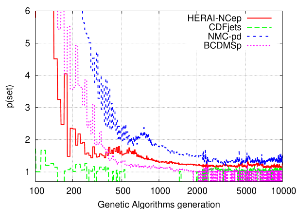
As an illustration of our procedure, we show in Fig. 7 the $p_{i}^{(k)}$ weight profiles as a function of the number of genetic algorithm generations for some sets of a given typical replica. Note how, at the early stages of the minimization, sets which are harder to learn, such as BCDMSp or NMC-pd are given more weight than the rest, while at the end of the weighted training epoch all weights are either $p_{i}^{(k)}\sim 1$ or oscillate between 0 and 1, a sign that these sets have been properly learnt.

The targeted weighted training epoch lasts for $N_{\rm gen}^{\rm wt}$ generations, unless the total error function Eq. (49) is above some threshold $E^{(k)}\geq E^{\mathrm{sw}}$. If it is, weighted training continues until $E^{(k)}$ falls below the threshold value. Afterwards, the error function is just the unweighted error function Eq. (49) computed on experiments. In this final training epoch, a dynamical stopping of the minimization is activated, as we shall discuss in the next section. Going through a final training epoch with the unweighted error function is in principle important in order to eliminate any possible residual bias from the choice of $E_{i}^{\rm targ}$ values in the previous epoch. However, in practice this safeguard has little effect, as it turns out that all weights tend to unity at the end of the targeted weighted training epoch as they ought to. The whole procedure ensures that a uniform quality of the fit for all datasets is achieved, and that the fit is refined using the correct figure of merit which includes all the information on correlated systematics.

Figure 7: Illustration of the weighted training in one particular replica. Individual weights for each dataset converge to a value of $p_{i}$ which is close to 1 as the training progresses. Only the behaviour of representative datasets is shown.

4.3 Genetic algorithm parameters

Genetic algorithms are controlled by some parameters that can be tuned in order to optimize the efficiency of the whole minimization procedure. The creation of new candidate PDFs that can lower the figure of merit used in the minimization is implemented using mutations. That is, each PDF is modified by changing some of the parameters that define the neural network. In this work, the initial mutation rates $\eta_{i,j}^{(0)}$, where $i$ labels the PDF and $j$ the specific mutation within this PDF, for the individual PDFs are kept the same as in [4, 6]. As training proceeds, all mutation rates are adjusted dynamically as a function of the number of iterations $N_{\rm ite}$

$$\eta_{i,j}=\eta_{i,j}^{(0)}/N_{\rm ite}^{r_{\eta}}\ .$$ (51)

In order to optimally span the range of all possible beneficial mutations, we introduce an exponent $r_{\eta}$ which is randomized between 0 and 1 at each interation of the genetic algorithm. An analysis of the values of $r_{\eta}$ for which mutations are accepted in each generation reveals a flat profile: both large and small mutations are beneficial at all stages of the minimization.

The number of mutants (new candidate solutions) in each genetic algorithm generation depends on the stage of the training. When the number of generations is smaller than $N_{\rm gen}^{\rm mut}$, we use a large population of mutants $N_{\rm mut}^{a}\gg 1$, while afterwards we use a much reduced population $N_{\rm mut}^{b}\ll N_{\rm mut}^{a}$. The rationale for this procedure is that at early stages of the minimization it is beneficial to explore as large a parameter space as possible, thus we need a large population. Once we are closer to a minimum, a reduced population helps in propagating the beneficial mutations to further improve the fitness of the best candidates. The final choices of parameters of the genetic algorithm which have been adopted in the NNPDF2.0 parton determination are summarized in Table 6.

$N_{\rm gen}^{\rm wt}$	$N_{\rm gen}^{\rm mut}$	$N_{\rm gen}^{\rm max}$	$E^{\mathrm{sw}}$	$N_{\rm mut}^{a}$	$N_{\rm mut}^{b}$
$10000$	2500	30000	2.6	80	10

Table 6: Parameter values for the genetic algorithm.

4.4 Preprocessing

Neural networks can accommodate any functional form, provided they are made of a large number of layers and sufficient time is used to train them. Nevertheless, it is customary to use preprocessing of data to subtract some dominant functional dependence. Then, smaller neural networks can be trained in a short time to deal with the deviations with respect to the dominant function. In our case, we use preprocessing to divide out some of the asymptotic small and large $x$ behaviour of PDFs. We avoid possible bias related to this by exploring a large space of preprocessing functions.

In this work, preprocessing is implemented in the way described in Sect. 3.1 of Ref. [6], to which we refer for a more detailed discussion. However, we now adopt in the fit a wider randomized range of variation of preprocessing exponents, thus ensuring greater stability and lack of bias. The range of preprocessing exponents used here is shown in Table 7.

The explicit independence of results on preprocessing exponents within the ranges defined in Table 7 can be verified by computing the correlation between the value of a given preprocessing exponent and the associated value of the $\chi^{2}$ computed between the $k$–th net and experimental data, defined by

$$\chi^{2(k)}={{1}\over{N_{\mathrm{dat}}}}\sum_{I,J=1}^{N_{\rm dat}}\left(F_{I}^{(\mathrm{exp})}-F_{I}^{(\mathrm{net})(k)}\right)\left(\left({\mathrm{cov}}\right)^{-1}\right)_{IJ}\left(F_{J}^{(\mathrm{exp})}-F_{J}^{(\mathrm{net})(k)}\right)\ .$$ (52)

Note that we always include a factor ${{1}\over{N_{\mathrm{dat}}}}$ in the definition of the $\chi^{2}$. Also, note that $\left(\left({\mathrm{cov}}\right)^{-1}\right)_{IJ}$ is the standard covariance matrix, which differs from the $t_{0}$–covariance matrix Eq. (1) because of the replacement of $F_{I}^{(0)}$,$F_{J}^{(0)}$ with the measured values $F_{I}$,$F_{J}$ in the second term on the right–hand side.

Therefore, we define the correlation coefficient as follows: considering for definiteness the large–$x$ preprocessing exponent of the singlet PDF $\Sigma(x,Q^{2})$, we have

$$r\left[\chi^{2},m_{\Sigma}\right]\equiv{{\left\langle\chi^{2}m_{\Sigma}\right\rangle_{\rm rep}-\left\langle\chi^{2}\right\rangle_{\rm rep}\left\langle m_{\Sigma}\right\rangle_{\rm rep}}\over{\sigma_{m_{\Sigma}}^{2}}}\ .$$ (53)

This provides the variation $\delta\chi^{2}$ as the large–$x$ exponent $\delta m_{\Sigma}$ is varied around its mean value. The correlations we find are very weak as shown in the last two columns of Table 7. It is clear that the $\chi^{2(k)}$ for the individual replicas is only marginally affected. This validates quantitatively the stability of our results with respect to the preprocessing exponents.

PDF	$\left[m_{\rm min},m_{\rm max}\right]$	$\left[n_{\rm min},n_{\rm max}\right]$	$r\left[\chi^{2},m\right]$	$r\left[\chi^{2},n\right]$
$\Sigma(x,Q_{0}^{2})$	$\left[2.55,3.45\right]$	$\left[1.05,1.35\right]$	-0.018	0.131
$g(x,Q_{0}^{2})$	$\left[1.05,1.35\right]$	$\left[1.05,1.35\right]$	-0.002	0.050
$T_{3}(x,Q_{0}^{2})$	$\left[2.55,3.45\right]$	$\left[0,0.5\right]$	-0.023	-0.130
$V_{T}(x,Q_{0}^{2})$	$\left[2.55,3.45\right]$	$\left[0,0.5\right]$	0.003	-0.068
$\Delta_{S}(x,Q_{0}^{2})$	$\left[12,14\right]$	$\left[-0.95,-0.65\right]$	0.000	-0.069
$s^{+}(x,Q_{0}^{2})$	$\left[2.55,3.45\right]$	$\left[1.05,1.35\right]$	0.021	-0.055
$s^{-}(x,Q_{0}^{2})$	$\left[2.55,3.45\right]$	$\left[0,0.5\right]$	-0.027	-0.015

Table 7: The range of random variation of the large-$x$ and small-$x$ preprocessing exponents $m$ and $n$ used in the present analysis (the precise form of these exponents is given in Sect. 3.1 of Ref. [6]). The last two columns give the correlation coefficient Eq. (53) between the $\chi^{2}$ and respectively the large and small–$x$ preprocessing exponents.

4.5 Positivity constraints

General theoretical constraints can be imposed during the minimization procedure, thereby guaranteeing that the fitting procedure only explores the subspace of acceptable physical solutions: for example, the valence and momentum sum rules are enforced in this way [4]. An important theoretical constraint is the positivity of physical cross–sections. As discussed in Ref. [60], positivity should be imposed on observable hadronic cross–sections and not on partonic quantities, which do not necessarily satisfy this constraint.

As in Ref. [4], positivity constraints on relevant physical observables have been imposed during the genetic algorithm minimization using a Lagrange multiplier, which strongly penalizes those PDF configurations which lead to negative observables. In particular, we impose positivity of $F_{L}(x,Q^{2})$, which constrains the gluon and the singlet PDFs at small–$x$, as well as that of the dimuon cross section $d^{2}\sigma^{\nu,c}/dxdy$ [6], which constrains the strange PDFs. Positivity should hold for any physical cross section which may be measured in principle. In practice, most PDFs are already well constrained by actual data, so that positivity is only relevant for PDFs such as the gluon and the strange distributions which are poorly constrained by the data.

Due to the positivity constraints, the minimized error function Eq. (49) (or Eq. (50) in the weighted training epoch) is modified as follows

$$E^{(k)}\to E^{(k)}-\lambda_{\rm pos}\sum_{I=1}^{N_{\rm dat,pos}}\Theta\left(-F_{I}^{({\rm net})(k)}\right)F_{I}^{({\rm net})(k)}\,,$$ (54)

where $N_{\rm dat,pos}$ is the number of pseudodata points used to implement the positivity constraints and we choose $\lambda_{\rm pos}\sim 10^{10}$ as its associate Lagrange multiplier. Positivity of $F_{L}(x,Q^{2})$ is implemented in the range $10^{-9}\leq x\leq 0.005$ and that of the dimuon cross section in $10^{-9}\leq x\leq 0.5$, in both cases at the initial evolution scale $Q^{2}=2$ GeV². This is done because if positivity is enforced at low scales, it will be preserved by DGLAP evolution.

The impact of the positivity constraints on the NNPDF2.0 PDF determination will be quantified in Sect. 5.5.

4.6 Determination of the optimal fit

We now turn to the formulation of the stopping criterion, which is designed to stop the fit at the point where the fit reproduces the information contained in the data but not its statistical fluctuations. The stopping criterion is applied on the training of each replica, and it is based on the cross–validation method, widely used in the context of neural network training [57]. Its application to our case has been described in detail in Refs. [3, 4], so here will mainly focus on the modifications introduced for NNPDF2.0.

As discussed in the previous section, dynamical stopping is activated after $N_{\rm gen}^{\rm wt}$ generations of targeted weighted training. Then, the weighted training on sets is switched off and minimization is done using Eq. (49) evaluated with the error function based on equally weighted experiments. The dynamical stopping criterion is only activated if a number of prior conditions are fulfilled. We first require that all experiments have an error function below some reasonable threshold $E_{\mathrm{thres}}$. Then, it is necessary that a moving average over the error function for the training and validation sets satisfy

$$r_{\mathrm{tr}}>1-\delta_{\rm tr};\quad r_{\mathrm{val}}>1+\delta_{\rm val},$$ (55)

where

$$r_{\rm tr}\equiv{{\langle E_{\mathrm{tr}}(i)\rangle}\over{\langle E_{\mathrm{tr}}(i-\Delta_{\mathrm{smear}})\rangle}}\,,$$ (56)

$$r_{\rm val}\equiv{{\langle E_{\mathrm{val}}(i)\rangle}\over{\langle E_{\mathrm{val}}(i-\Delta_{\mathrm{smear}})\rangle}}\,.$$ (57)

where the smeared error functions are given by

$$\langle E_{\mathrm{tr,val}}(i)\rangle\equiv{{1}\over{N_{\mathrm{smear}}}}\sum_{l=i-N_{\mathrm{smear}}+1}^{i}E_{\mathrm{tr,val}}(l)\,,$$ (58)

with $E_{\mathrm{tr,val}}(l)$ being the figure of merit Eq. (49) restricted to the training and validation sets for the genetic algorithms generation $l$.

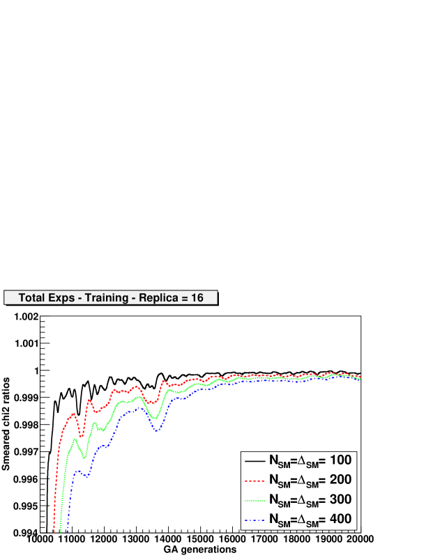
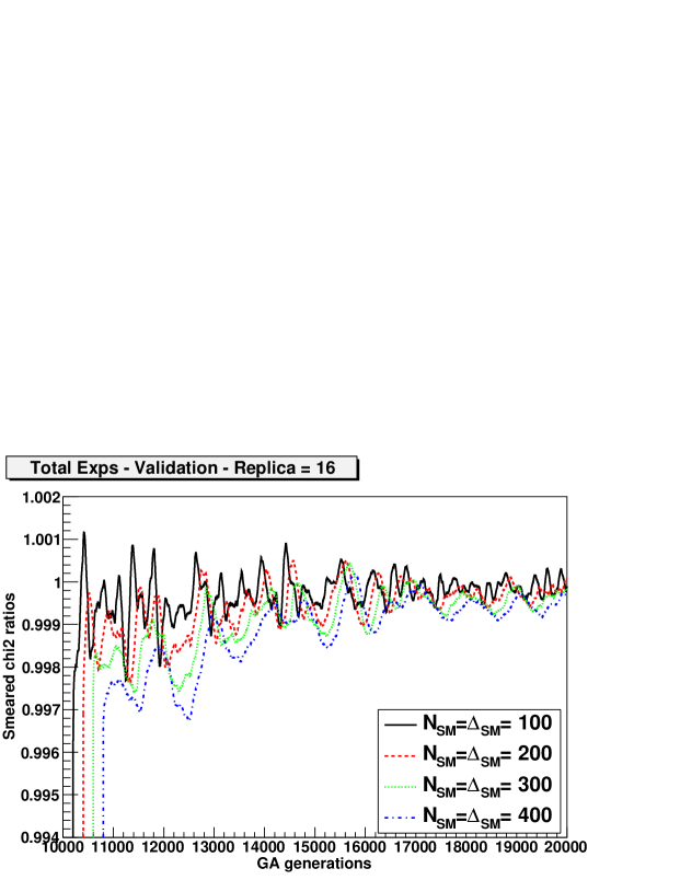
The values of the stopping parameters $\delta_{\rm tr}$ and $\delta_{\rm val}$ must be determined by analyzing the behaviour of the fit for the particular dataset which is being used for neural network training. As an illustration of how this is done in practice, we show in Fig. 8 the averaged training and validation $E_{\rm tr/val}$ ratios Eqs. (56-57) for a given replica and different values of the smearing length $N_{\rm smear}$. For this particular replica the training has been artificially prolonged beyond its stopping point. From Fig. 8 it is apparent that while the training ratio satisfies $r_{\mathrm{tr}}<1$ always, i.e. that $E^{(k)}_{\rm tr}$ continues to decrease, after a given number of generations we have $r_{\mathrm{val}}>1$, which then oscillates above and below 1: this is the sign that we have entered an ‘overlearning’ regime and minimization needs to be stopped.

The optimal values of the stopping parameters are chosen to be small enough that overlearning is avoided, but large enough that the fit does not stop on statistical fluctuations. The latter condition can be met only if the value of $N_{\rm smear}$ is large enough, but if $N_{\rm smear}$ is too large stopping becomes very difficult and the first condition cannot be met. In practice, we have produced a set of 100 replicas with very long training, and for each value of $N_{\rm smear}$ we have tried out a range of values of $\delta_{\rm tr}$ and $\delta_{\rm val}$, until an optimal set of values which satisfies all the above criteria has been found. The final values of the parameters determined in this way are listed in Table 8. In order to avoid unacceptably long fits, when a very large number of iterations $N_{\rm gen}^{\rm max}$ is reached (see Table 6) training is stopped anyway. This leads to a small loss of accuracy of the corresponding fits which is acceptable provided it only happens for a small fraction of replicas.

$N_{\mathrm{smear}}$	$\Delta_{\mathrm{smear}}$	$\delta_{\rm tr}$	$\delta_{\rm val}$	$E_{\mathrm{thres}}$	$N_{\rm gen}^{\rm max}$
$200$	$200$	$10^{-4}$	$3\,10^{-4}$	6	30000

Table 8: Parameter values for the stopping criterion.

Figure 8: The training (upper plot) and validation (lower plot) ratios Eqs. (56- 57) for a particular replica, as a function of the number of genetic algorithms generations, for various choices of the smearing parameter $N_{\rm smear}=\Delta_{\rm smear}$. The value $N_{\rm smear}=\Delta_{\rm smear}=200$ is used in the reference fit (see Table 8).

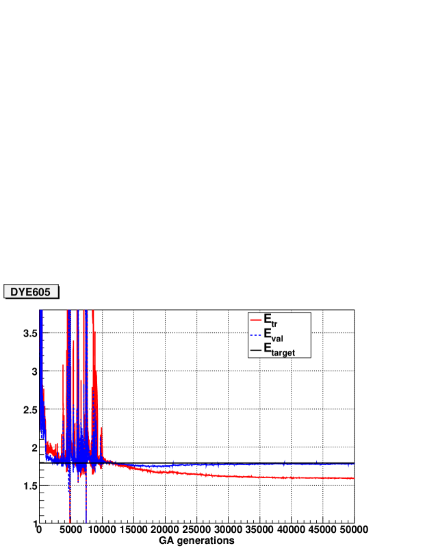
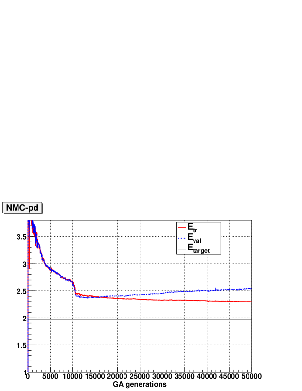
In order to check the consistency of the whole procedure, we have produced a set of 100 replicas from a fit with the same settings as the final reference fit but with no stopping and a large maximum number of genetic algorithm generations $N_{\rm gen}^{\rm max}=50000$. This set of 100 replicas allows us thus to verify that the targeted weighted training and stopping criterion do not bias the fitting procedure, in that the values of $E_{j}^{(k)}$ do not drift away from the target values $E_{j}^{\rm targ}$ when the weighted training is switched off, and also that the stopping criterion does not introduce underlearning by stopping the fit at a time when the quality of the fit is still improving. These conclusions are borne out, and in fact, in these fits for many experiments and replicas the value of $E_{j}^{(k)}$ changes very little after the target values $E_{j}^{\rm targ}$ are reached — indeed, the target values were obtained from a very long fit in the first place. Indeed, the average $\chi^{2}$ for this fit is only marginally better than that of the reference fit. However, some experiments do show signs of overlearning, with an accordingly lower value of the contribution to the $\chi^{2}$ .

This is illustrated in Fig. 9, where we show the $E^{(k)}_{i}$ profiles for two particular experiments (E605 and NMC-pd) and replicas taken from this fit without stopping. In the first training epoch, in which the weighted training Eq. (50) is activated, one can see oscillations, but the downwards trend is clearly visible. Once targeted weighted training is switched off, minimization proceeds smoothly, and we see in the two cases that after a given number of genetic algorithms generations we enter in overlearning. For the two experiments the typical overlearning behaviour, characterized by the fact that the validation $E^{(k)}_{\rm tr}$ is rising while the training $E^{(k)}_{\rm val}$ is still decreasing, sets in at about 15000 generations. This is the point where dynamical stopping avoids overlearning.

Figure 9: Two typical examples of overlearning behaviour, extracted from a fit with the same settings as the final reference fit but with no stopping and a large maximum number of genetic algorithm generations $N_{\rm gen}^{\rm max}=50000$. The upper plot shows the overlearning of the E605 experiment observed in one particular replica, and the lower plot corresponds to the NMC-pd experiment. Note that in these fits weighted training is switched off at $N_{\rm gen}^{\rm wt}=10000$.

5 Results

In this section we present the NNPDF2.0 parton determination. First we discuss the statistical features of the fit, then we turn to a comparison of NNPDF2.0 PDFs and uncertainties with other PDF determinations and with previous NNPDF releases. Next we turn to a study of potential deviations from gaussian behaviour in PDF uncertainty bands. A detailed comparison between NNPDF2.0 and NNPDF1.2 follows, in which the impact of each of the differences between these fits is studied in turn: improved neural network training, treatment of normalization uncertainties, impact of the combined HERA-I dataset, impact of the inclusion of jet and Drell-Yan data. Finally we discuss the impact of the positivity constraints in the PDF determination, and study the sensitivity of NNPDF2.0 to variations in the value of the strong coupling $\alpha_{s}$.

Note that while results for the NNPDF2.0 fit are obtained with $N_{\rm rep}=1000$ replicas, those for all other comparisons performed here are done with $N_{\rm rep}=100$ replicas.

5.1 NNPDF2.0: statistical features

$\chi^{2}_{\mathrm{tot}}$	1.21
$\left\langle E\right\rangle\pm\sigma_{E}$	2.32 $\pm$ 0.10
$\left\langle E_{\rm tr}\right\rangle\pm\sigma_{E_{\rm tr}}$	2.29 $\pm$ 0.11
$\left\langle E_{\rm val}\right\rangle\pm\sigma_{E_{\rm val}}$	2.35 $\pm$ 0.12
$\left\langle{\rm TL}\right\rangle\pm\sigma_{\rm TL}$	16175 $\pm$ 6257
$\left\langle\chi^{2(k)}\right\rangle\pm\sigma_{\chi^{2}}$	1.29 $\pm$ 0.09
$\left\langle\sigma^{(\exp)}\right\rangle_{\mathrm{dat}}$(%)	11.4
$\left\langle\sigma^{(\mathrm{net})}\right\rangle_{\mathrm{dat}}$(%)	6.0
$\left\langle\rho^{(\exp)}\right\rangle_{\mathrm{dat}}$	0.18
$\left\langle\rho^{(\mathrm{net})}\right\rangle_{\mathrm{dat}}$	0.54

Table 9: Table of statistical estimators for NNPDF2.0 with $N_{\rm rep}=1000$ replicas. The total average uncertainty is given in percentage.

Experiment	$\chi^{2}$	$\left\langle E\right\rangle$	$\left\langle\sigma^{(\exp)}\right\rangle_{\mathrm{dat}}$(%)	$\left\langle\sigma^{(\mathrm{net})}\right\rangle_{\mathrm{dat}}$(%)	$\left\langle\rho^{(\exp)}\right\rangle_{\mathrm{dat}}$	$\left\langle\rho^{(\mathrm{net})}\right\rangle_{\mathrm{dat}}$
NMC-pd	0.99	2.05	1.8	0.5	0.03	0.36
NMC	1.69	2.79	4.9	1.7	0.16	0.77
SLAC	1.34	2.42	4.2	1.9	0.31	0.84
BCDMS	1.27	2.40	5.7	2.6	0.47	0.55
HERAI-AV	1.14	2.25	7.5	1.3	0.06	0.44
CHORUS	1.18	2.32	14.8	12.8	0.09	0.38
FLH108	1.49	2.51	71.9	3.3	0.65	0.68
NTVDMN	0.67	1.90	21.1	14.6	0.03	0.63
ZEUS-H2	1.51	2.66	13.6	1.2	0.29	0.58
DYE605	0.88	1.85	22.6	8.3	0.47	0.75
DYE866	1.28	2.35	20.8	9.1	0.20	0.45
CDFWASY	1.85	3.09	6.0	4.3	0.52	0.72
CDFZRAP	2.02	2.96	11.5	3.5	0.83	0.65
D0ZRAP	0.57	1.65	10.2	3.0	0.53	0.69
CDFR2KT	0.80	2.22	23.0	5.2	0.78	0.67
D0R2CON	0.93	1.92	16.2	6.0	0.78	0.64

Table 10: Same as Table 9 for individual individual experiments. Note that experimental uncertainties are always given in percentage.

The statistical features of the NNPDF2.0 analysis are summarized in Tables 9 (for the total dataset) and 10 (for individual experiments). Note that $E^{(k)}$ Eq. (49) and ${\chi^{2}}^{(k)}$ Eq. (52) differ both because in the former each PDF replica is compared to the data replica it is fitted to, while in the latter it is compared to the actual data, and also because of the different treatment of normalization uncertainties as discussed after Eq. (52). The value of $\chi^{2}_{\mathrm{tot}}$ then refers to the average over replicas (best fit PDF set), while the value $\left\langle\chi^{2(k)}_{\mathrm{tot}}\right\rangle$ is the average (and associate standard deviation) of ${\chi^{2}}^{(k)}$ computed for each replica. The average training length $\langle TL\rangle$ (expressed as a number of generations of the genetic algorithm) is also given in this table.

Figure 10: Distribution of $\chi^{2(k)}$ Eq. (52) (left) and $E^{(k)}_{\rm tr}$ Eq. (49) over the sample of $N_{\mathrm{r}ep}=1000$ replicas.

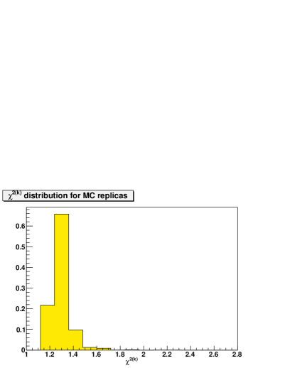
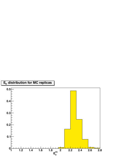
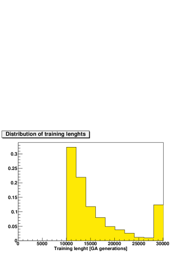
The distribution of $\chi^{2(k)}$ Eq. (52), $E^{(k)}_{\rm tr}$ Eq. (49) and training lengths among the $N_{\rm rep}=1000$ replicas are shown in Fig. 10 and Fig. 11 respectively. While most of the replicas fulfill the stopping criterion, a small fraction ($\sim 12\%$) of them stop at the maximum training length $N_{\rm gen}^{\rm max}$ which, as discussed in Sect. 4.6, has been introduced in order to avoid unacceptably long fits. This causes some loss of accuracy in outliying fits, but we have checked that as $N_{\rm gen}^{\rm max}$ is raised more and more of these replicas would eventually stop, and that the loss of accuracy due to this choice of value of $N_{\rm gen}^{\rm max}$ is actually very small.

Figure 11: Distribution of training lengths over the sample of $N_{\mathrm{r}ep}=1000$ replicas.

The features of the fit can be summarized as follows:

• As in previous fits, the values of $\chi^{2}_{\mathrm{tot}}$ and $\left\langle E\right\rangle$ differ by about one unit, consistent with the expectation that the best fit correctly reproduces the underlying true behaviour about which data fluctuate, with replicas further fluctuating about data. Interestingly, much of the replica fluctuation is already removed by neural network training, i.e. when going from $\left\langle E\right\rangle$ to $\left\langle\chi^{2(k)}\right\rangle$, with only a further small amount of statistical fluctuation being removed when averaging over replicas to get the best–fit $\chi_{\mathrm{tot}}$. This reduction was already present in NNPDF1.2 (see the first column of Tab. 11 below), where however both $\left\langle\chi^{2(k)}\right\rangle$ and $\left\langle E\right\rangle$ differed rather more from the best fit $\chi^{2}_{\mathrm{tot}}$ and from each other. The improvement shows that the training and stopping algorithm used here and described in Sect. 4 are more efficient.

• The quality of the fit as measured by its $\chi^{2}_{\rm tot}=1.21$ has improved in comparison to NNPDF1.2 [6] despite the widening of the dataset to also include hadronic data. As we will discuss in greater detail in Sect. 5.4 below (see in particular Tab. 11) this improvement is largely due to the improvement in training and stopping, and to a lesser extent to the improved treatment of normalization uncertainties. The inclusion of the very precise combined HERA data then leads to a small deterioration in fit quality (possibly because of the lack of inclusion of charm mass effects near charm threshold), while the jet and DY data do not lead to any further deterioration. This $\chi^{2}$ value has very low gaussian probability and it is thus quite unlikely as a statistical fluctuation: it suggests experimental uncertainties might be underestimated at the 10% level, or that there might be theoretical uncertainties of the same order. This appears consistent with the expected accuracy of a NLO treatment of QCD, and the typical accuracy with which experimental uncertainties are estimated.

• The histogram of $\chi^{2}$ values for each experimental dataset is shown in Fig. 12, where the unweighted average $\left\langle\chi^{2}\right\rangle_{\rm sets}\equiv{{1}\over{N_{\rm set}}}\sum_{j=1}^{N_{\rm set}}\chi^{2}_{\rm set,j}$ and standard deviation over datasets are also shown. We see no evidence of any specific dataset being clearly inconsistent with the other, and the distribution of values looks broadly consistent with statistical expectations, with about five datasets with $\chi^{2}$ at more than one but less than two sigma from the average. Also, we see no obvious difference or tension between hadronic and DIS datasets. Clearly, the $\chi^{2}$ values for some experiments if taken at face value have low gaussian probabilities (though only one, namely NMC, has a probability less than 0.01%). However, they appear to be stable upon the inclusion of new data, thus suggesting a lack of tension between different datasets. For instance, the $\chi^{2}$ value of the NMC data is very close to that of Refs. [1, 2]: this value thus appears to reflect the internal consistency of these data, not their consistency with other data. Some of the issues with specific datasets will be discussed in somewhat greater detail in this section below, while the behaviour of the fit quality as more data are included in the fit will be discussed in detail in Sect. 5.4, where strong evidence for the lack of tension between datasets will be presented.

• As in previous NNPDF determinations, the uncertainty of the fit, as measured by the average standard deviation $\langle\sigma\rangle$ is rather smaller than that of the data: 6.0% vs. 11.4%. The uncertainty reduction shows that the PDF determination is combining the information contained in the data into a determination of an underlying physical law. As one would expect the greatest reduction is observed in HERA DIS data, but sizable reductions are also seen in Drell-Yan and jet data, thus confirming the consistency of these data with the global dataset.

Figure 12: Values of the $\chi^{2}$ (or more properly the $\chi^{2}$ per data point - see Eq.(52)) for the datasets included in the NNPDF2.0 reference fit, listed in Table 10. The horizontal line corresponds to the unweighted average of these $\chi^{2}$ over the datasets and and the black dashed line to the one–sigma interval about it: $\left\langle\chi^{2}\right\rangle_{\rm sets}=1.06$, $\sigma_{\chi^{2}}=0.40$; DIS and hadronic datasets are grouped respectively to the left and right of the histogram and distinguished by different colors.

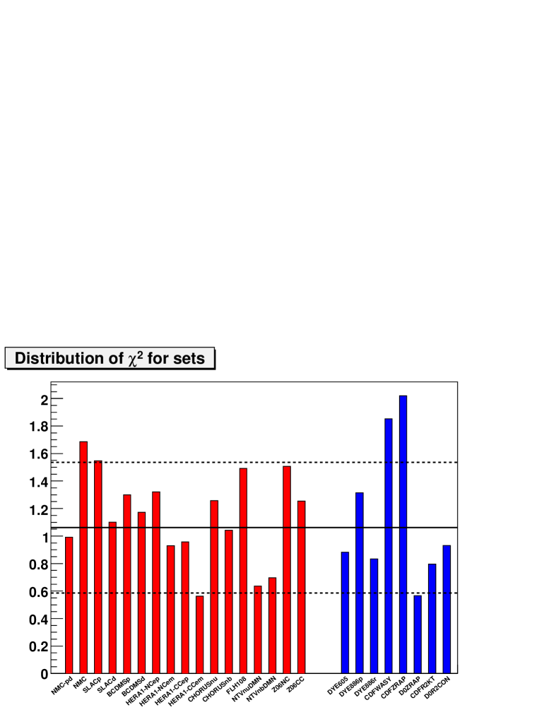
Let us now consider in greater detail the quality of the fit for some specific experiments whose $\chi^{2}$ differs by more than one sigma from the average:

• The high value of the $\chi^{2}$ of the NMC $F_{2}^{p}$ data has been observed in all our previous PDF determinations. It should be observed that, as already mentioned, it was first observed in Refs. [1, 2], where a parametrization of the structure function $F_{2}^{p}(x,Q^{2})$ was constructed without using either PDFs or QCD: hence, this value simply reflects the fact that the data within this set are not consistent with each other, i.e. they show point-by-point fluctuations which are wider than allowed by their declared uncertainty.

• For dimuon data $\chi^{2}\sim 0.65$, as was also the case in NNPDF1.2 [6]. As discussed there in detail, this stems from the fact that statistical and systematic uncertainties are added in quadrature for this dataset: the dominant statistical uncertainty is affected by a bin by bin correlation due to the unfolding procedure used in extracting the dimuon cross section from the measured observable, but the corresponding covariance matrix is not available.

• The $\chi^{2}$ of the HERA-I combined data is $\chi^{2}=1.14$, somewhat larger than the value found when fitting the separate ZEUS and H1 data. The value comes from averaging the relatively large $\chi^{2}\sim 1.3$ for the very precise NC positron dataset, with a low value $\chi^{2}\sim 0.6$ for CC electron data. The reasons for this distribution of values are unclear, however, we note that also in NNPDF1.2 [6] the $\chi^{2}$ of the CC datasets was typically smaller than the average as well. We note also that the same pattern of $\chi^{2}$ among the different datasets has been obtained within the framework of the HERAPDF1.0 analysis of these combined HERA-I dataset [12, 61].

• The CDF direct $W-$asymmetry measurements have $\chi^{2}=1.85$. The poor compatibility of these data with the rest of the global fit data was also noted in the global analysis of Refs. [62, 63].

• The quality of the fit to Z rapidity distribution data at the Tevatron differs widely between experiments: while an excellent fit is obtained for D0 data, CDF data are not so well described. This suggests that there might be problem of internal consistency between the two experiments. A similar pattern was observed in the MSTW08 global fit [11]. Note that these datasets have a very moderate impact on the global fit, as proven by the fact that (see Sect. 5.4 below, in particular Table 11) the $\chi^{2}$ of these data is essentially the same in NNPDF2.0 and in NNPDF1.2 (where they are not fitted).

Finally, we have checked that if we run a very long fit without dynamical stopping, the $\chi^{2}$ of the experiments whose values exceed the average by more than one sigma does not improve significantly. This shows that the deviation of these $\chi^{2}$ values from the average is not due to underlearning.

5.2 Parton distributions

Figure 13: The singlet $\Sigma=\sum_{i}(q_{i}+\bar{q_{i}})$, gluon $g$ and total strangeness $s^{+}=s+\bar{s}$ at the initial scale $Q_{0}^{2}=2$ GeV² from the NNPDF2.0 analysis both on linear (left) and logarithmic (right) scale, compared to the previous NNPDF releases NNPDF1.0 [4] and NNPDF 1.2 [6].

Figure 14: Same as Fig. 13 for the triplet $T_{3}=u+\bar{u}-d-\bar{d}$, total valence $V=\sum_{i}(q_{i}-\bar{q_{i}})$, sea asymmetry $\Delta_{S}=\bar{d}-\bar{u}$ and strangeness asymmetry $s^{-}=s-\bar{s}$.

Figure 15: Absolute uncertainties on the PDFs of Fig. 13.

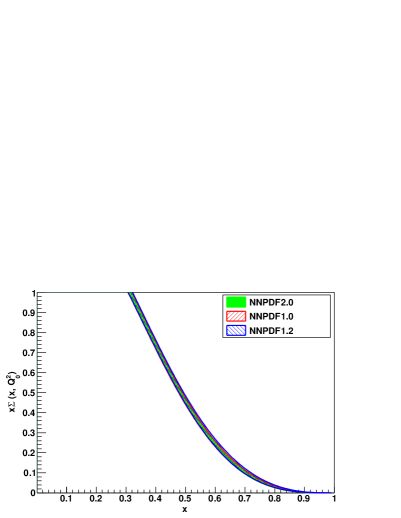
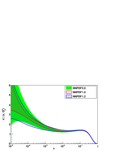
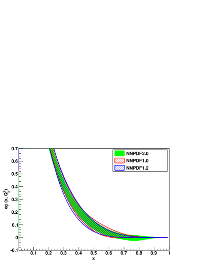
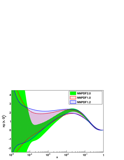
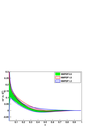
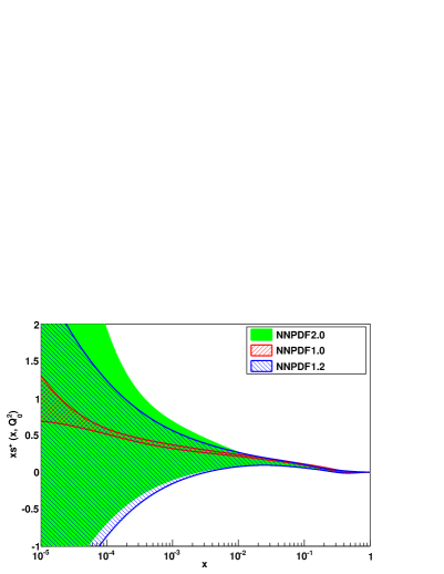
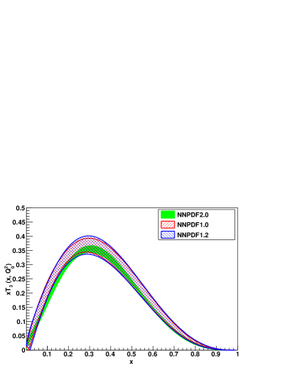
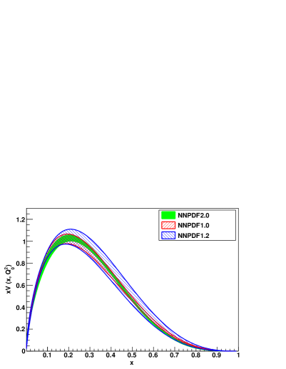
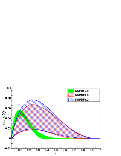
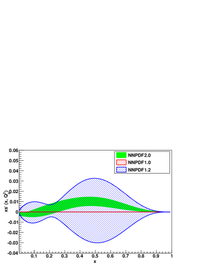
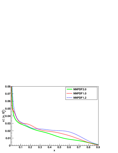
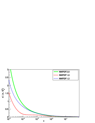
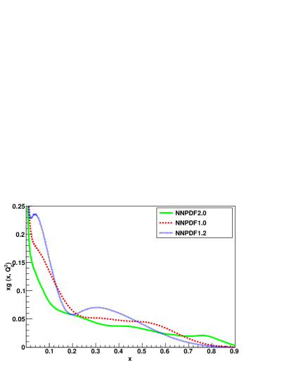
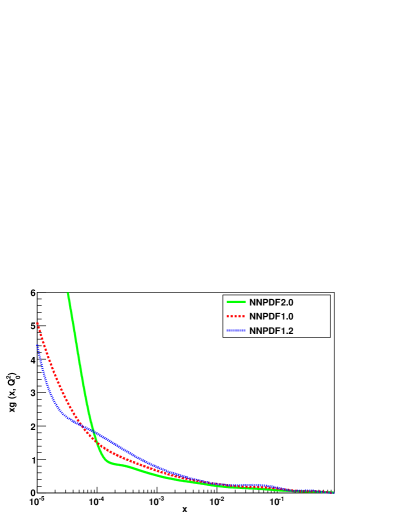
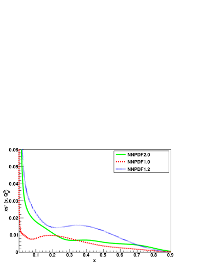
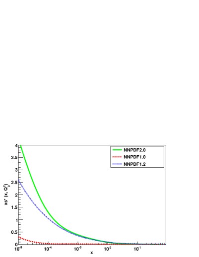
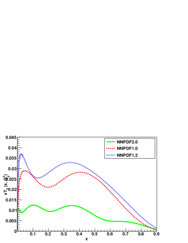
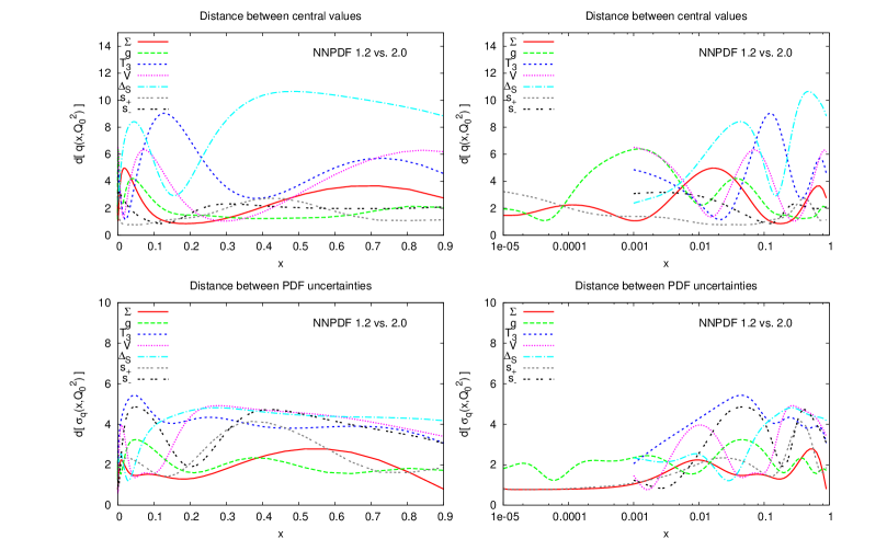
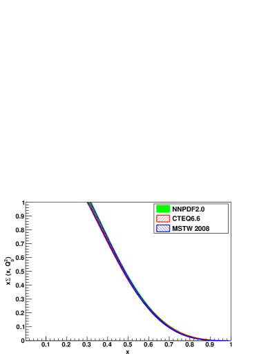
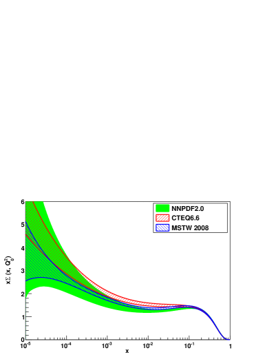
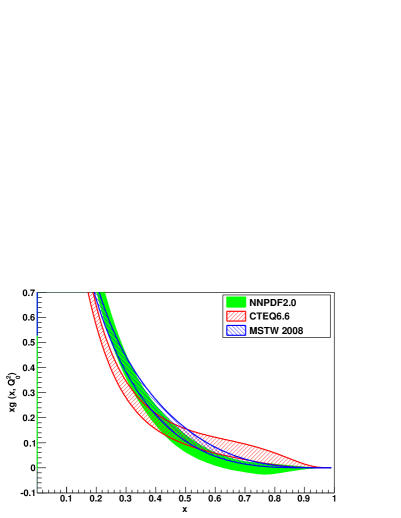
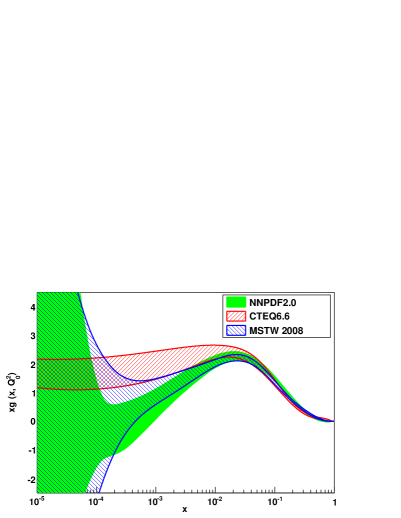
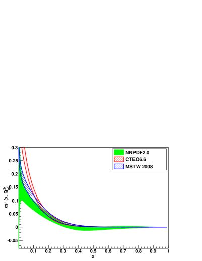
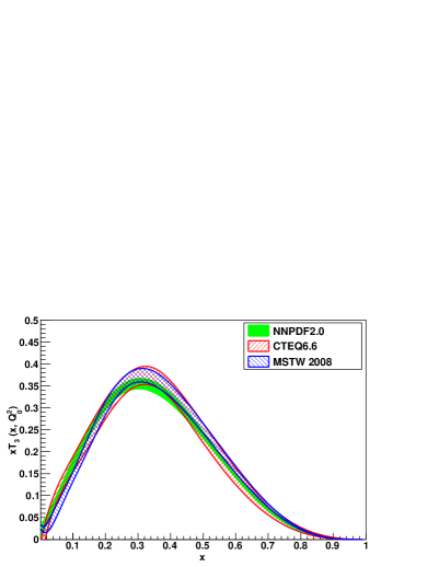
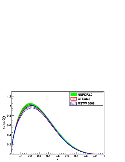
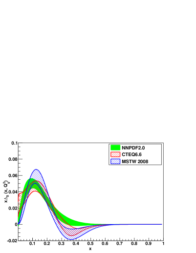
The NNPDF2.0 PDFs are compared to the previous NNPDF1.0 [4] and NNPDF1.2 [6] parton sets in Figs. 13–16. All PDF combinations are defined as in Refs. [4, 6]. Note that all uncertainty bands shown are one–sigma; the relation to 68% confidence levels will be discussed in Sect. 5.3 below. The consistency between subsequent NNPDF releases, extensively discussed in previous work [4, 6] is apparent. Also apparent is the reduction in uncertainty obtained going from NNPDF1.2 to NNPDF2.0; the causes for this improvement will be discussed in detail in Sect. 5.4 below. In order to further quantify the differences between the NNPDF2.0 and NNPDF1.2 parton sets, the distance (as defined in Appendix A) between these sets are shown in Fig 17 as a function of $x$: all PDFs for all $x$ are consistent at the 90% confidence level, and in fact almost all are consistent to within one sigma.

Figure 16: Absolute uncertainties on the PDFs of Fig. 14.

Figure 17: Distance between the NNPDF2.0 and the NNPDF1.2 parton sets (central values and uncertainties) for all PDFs as a function of $x$. All distances are computed from sets of $N_{\rm rep}=100$ replicas (see Appendix A.)

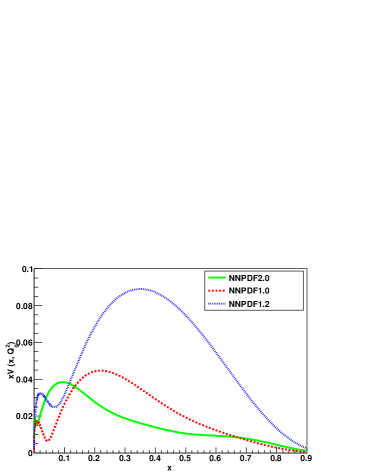
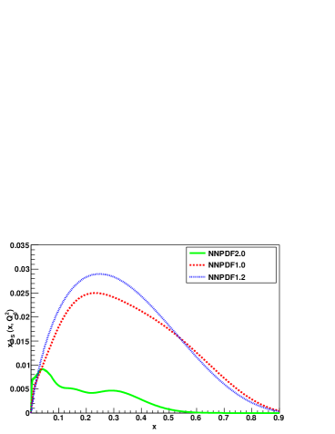
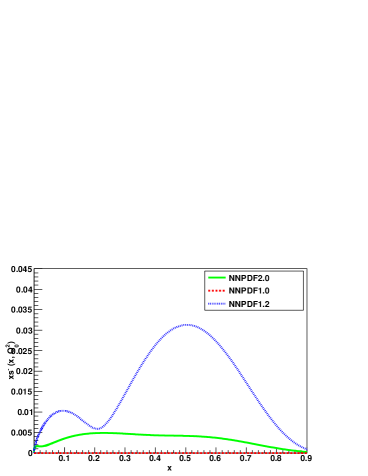
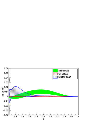
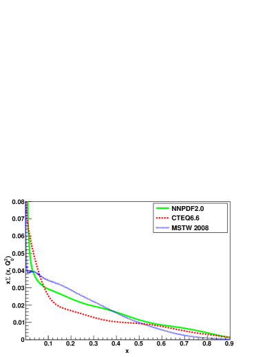
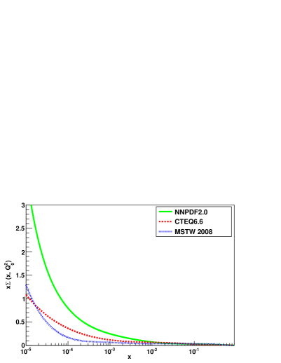
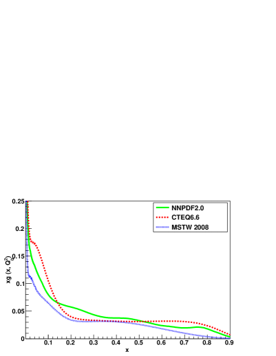
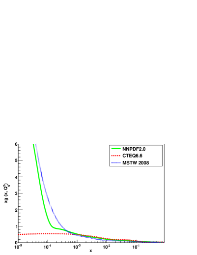
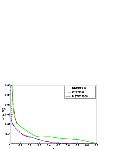
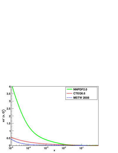
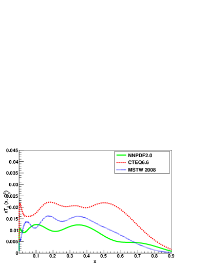
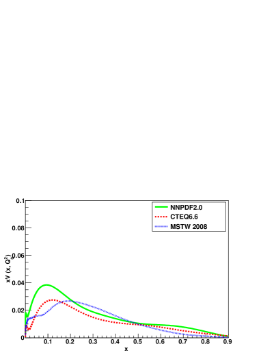
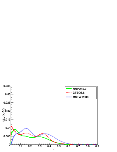
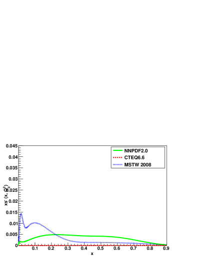
The NNPDF2.0 PDFs are also compared to CTEQ6.6 [10] and MSTW08 [11] PDFs in Figs. 18–21. Most NNPDF2.0 uncertainties are comparable to the CTEQ6.6 and MSTW08 ones; there are however some interesting exceptions. The uncertainty on strangeness, which NNPDF2.0 parametrizes with as many parameters as any other PDF, is rather larger than those of MSTW08 and CTEQ6.6, in which these PDFs are parametrized with a very small number of parameters. The NNPDF2.0 uncertainty on total quark singlet (which contains a sizable strange contribution) is also larger. The uncertainty on the small $x$ gluon is significantly larger than that found by CTEQ6.6, but comparable to that MSTW08, which has an extra parameter to describe the small $x$ gluon in comparison to CTEQ6.6. The uncertainty on the triplet combination is rather smaller in NNPDF2.0 than either MSTW08 or CTEQ6.6. As we shall see in Sect. 5.4, this small uncertainty is largely due to the impact of Drell-Yan data (which are found to be completely consistent with DIS data within our NLO treatment): hence, the fact that we find it to be smaller than MSTW08 or CTEQ6.6 does not appear to be due to the choice of dataset.

Figure 18: Same as Fig. 13, but compared to MSTW08 [11] and CTEQ6.6 [10] PDFs.

Figure 19: Same as Fig. 14, but compared to MSTW08 [11] and CTEQ6.6 [10] PDFs.

Figure 20: Same as Fig. 15, but compared to MSTW08 [11] and CTEQ6.6 [10] PDFs.

Figure 21: Same as Fig. 16, but compared to MSTW08 [11] and CTEQ6.6 [10] PDFs.

5.3 Confidence levels

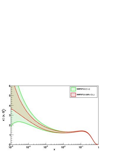
An important advantage of the Monte Carlo method used in the NNPDF approach to determine PDF uncertainties is that, unlike in a Hessian approach, one does not have to rely on linear error propagation. It is then possible to test the implication of a non-gaussian distribution of experimental data which were found in Ref. [64] to be minor; and and also to test for non-gaussian distribution of the fitted PDFs even though our starting data and data replicas are gaussianly distributed.

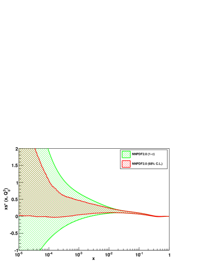
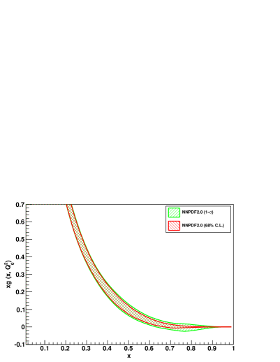
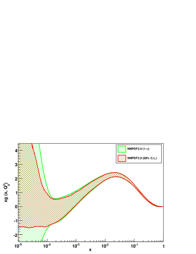
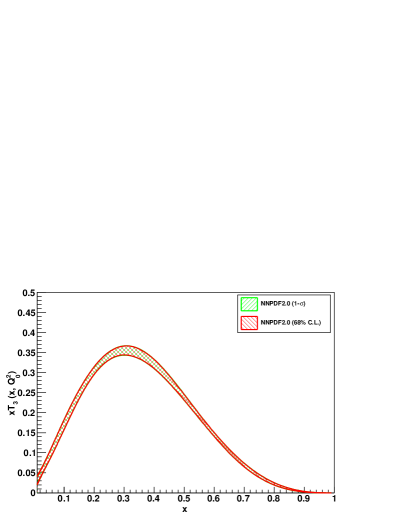
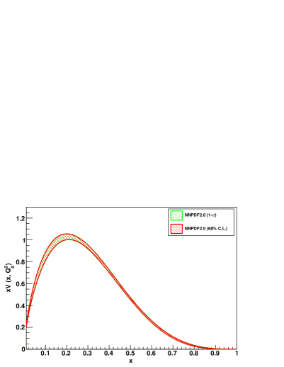
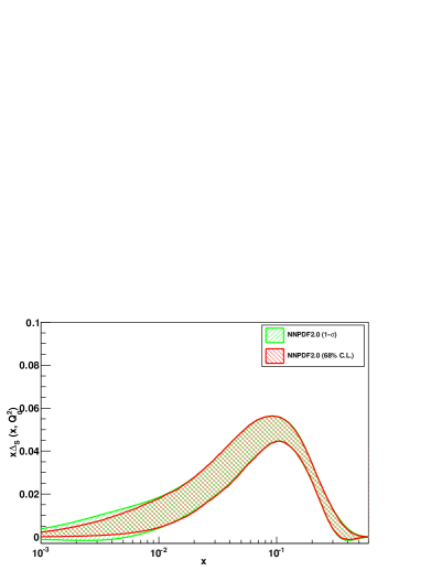
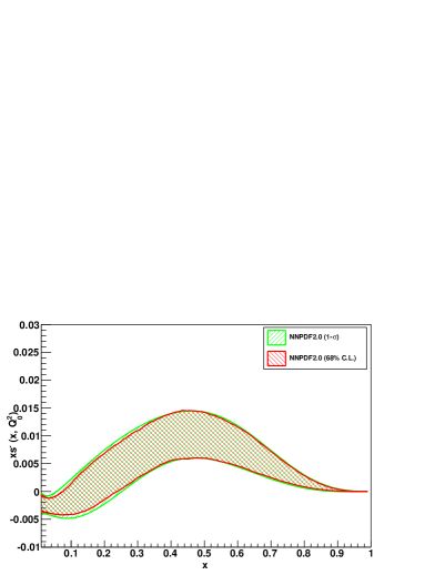
A simple way to test for non-gaussian behaviour for some quantity is to compute a 68% confidence level for it (which is straightforwardly done in a Monte Carlo approach), and compare the result to the standard deviation. This method was used in Ref. [6] to identify large departures from gaussian behaviour in the strange over non-strange momentum ratio. In Fig. 22 this comparison is shown for all NNPDF2.0 PDFs at the initial scale as a function of $x$.

Figure 22 shows that in the regions in which the PDFs are constrained by experimental data the standard deviation and the 68% confidence levels coincide to good approximation, thus suggesting gaussian behaviour. However, in the extrapolation region for most PDFs deviations from gaussian behaviour are sizable. This is especially noticeable for the gluon at small $x$, and for the quark singlet and total strangeness both at small and large $x$. Deviations from gaussian behaviour are sometimes related to positivity constraints Eq. (54): for instance positivity of $F_{L}$ and the dimuon cross–section limits the possibility for the small–$x$ gluon and strange sea PDFs respectively to go negative, thereby leading to an asymmetric uncertainty band. The impact of positivity constraints on PDFs will be discussed in greater detail in Sect. 5.5.

Figure 22: Comparison of 68% confidence level and one–sigma intervals for NNPDF2.0 PDFs at the initial scale.

Fit	NNPDF1.2	NNPDF1.2+IGA	NNPDF1.2+IGA+$t_{0}$	2.0 DIS	2.0 DIS+JET	NNPDF2.0
$\chi^{2}_{\mathrm{tot}}$	1.32	1.16	1.12	1.20	1.18	1.21
$\left\langle E\right\rangle$	2.79	2.41	2.24	2.31	2.28	2.32
$\left\langle E_{\rm tr}\right\rangle$	2.75	2.39	2.20	2.28	2.24	2.29
$\left\langle E_{\rm val}\right\rangle$	2.80	2.46	2.27	2.34	2.32	2.35
$\left\langle\chi^{2(k)}\right\rangle$	1.60	1.28	1.21	1.29	1.27	1.29
NMC-pd	1.48	0.97	0.87	0.85	0.86	0.99
NMC	1.68	1.72	1.65	1.69	1.66	1.69
SLAC	1.20	1.42	1.33	1.37	1.31	1.34
BCDMS	1.59	1.33	1.25	1.26	1.27	1.27
HERAI	1.05	0.98	0.96	1.13	1.13	1.14
CHORUS	1.39	1.13	1.12	1.13	1.11	1.18
FLH108	1.70	1.53	1.53	1.51	1.49	1.49
NTVDMN	0.64	0.81	0.71	0.71	0.75	0.67
ZEUS-H2	1.52	1.51	1.49	1.50	1.49	1.51
DYE605	11.19	22.89	8.21	7.32	10.35	0.88
DYE866	53.20	4.81	2.46	2.24	2.59	1.28
CDFWASY	26.76	28.22	20.32	13.06	14.13	1.85
CDFZRAP	1.65	4.61	3.13	3.12	3.31	2.02
D0ZRAP	0.56	0.80	0.65	0.65	0.68	0.57
CDFR2KT	1.10	0.95	0.78	0.91	0.79	0.80
D0R2CON	1.18	1.07	0.94	1.00	0.93	0.93

Table 11: Statistical estimators for the sequence of fits that take from NNPDF1.2 to NNPDF2.0. The estimators shown for NNPDF1.2 are as in Tab. 5-6 of Ref. [6] and those for NNPDF2.0 are as in Tab. 9–10. Estimators are shown for the total datasets in the upper part of the table, while the lower part of the table shows the $\chi^{2}$ for each individual experimental dataset. Values of the $\chi^{2}$ for data not included in any given fit are shown in italic; the total $\chi^{2}_{\rm tot}$ shown in the first line does not include the contribution from these data. The value of the $\chi^{2}$ in the HERAI line refers in the first three columns of the table to the weighted sum of the H1 and ZEUS data, and in the latter three columns to the combined dataset, according to which data has been included in the fit.

5.4 Detailed comparison to NNPDF1.2: methodology and dataset

As seen in Sect. 5.2 the quality of the NNPDF2.0 fit is rather better than that of NNPDF1.2, despite the wider dataset. We now perform a detailed comparison of these two fits, which differ both in procedural aspects and in dataset. In order to elucidate the impact on the fit of each of these, we have produced a sequence of PDF determinations that take us from NNPDF1.2 to NNPDF2.0 by varying one by one each of the procedural aspects, then each of the datasets inclusions, as follows

(i) we start from NNPDF1.2;

(ii) we switch to the improved genetic algorithm and minimization of Sect. 4 (IGA);

(iii) we introduce the improved treatment of normalization uncertainties of Ref. [18] ($t_{0}$ method);

(iv) we replace the separate H1 and ZEUS data with the new combined HERA-I dataset: this gives the NNPDF2.0 set, but with DIS data only (2.0-DIS);

(v) we add jet data (2.0-DIS+jet);

(vi) we add the DY data, thereby obtaining the NNPDF2.0 fit.

The statistical estimators for this sequence of fits are shown in Table 11 (including the NNPDF2.0 estimators already shown in Tab. 9–10). We will now discuss each of these subsequent fits in turn by examining its general features, and determining and understanding the distance (as defined in Appendix A) between PDFs obtained in each pair of subsequent fits.

1. Effect of the improved genetic algorithm and stopping criterion (IGA).
   The improvement in neural network training leads to a significant improvement in fit quality: each replica fits better the corresponding data replica (lower $\langle E\rangle$), and also each replica neural network is more efficient in subtracting the statistical noise from data (lower $\langle\chi^{2\,(k)}\rangle$), thereby leading to a better global fit (lower $\chi^{2}_{\rm tot}$). The improvement is due to the improvement in fit quality of fixed–target DIS experiments (NMC, BCDMS and CHORUS) which probe the valence region which has more structure, and which moreover are known [1, 2, 65] to have a certain amount of data inconsistency, without change in fit quality for other experiments: this means that the new algorithm is more efficient in leading to a balanced fit quality between experiments, without some data being underlearnt while others are overlearnt.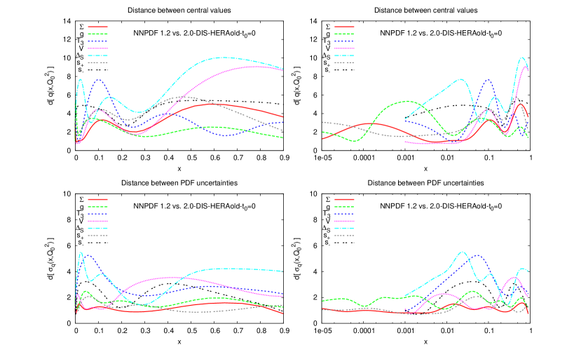

   

   Figure 23: Distance between the NNPDF1.2 fit and a fit to the same data but improved genetic algorithm and stopping (IGA).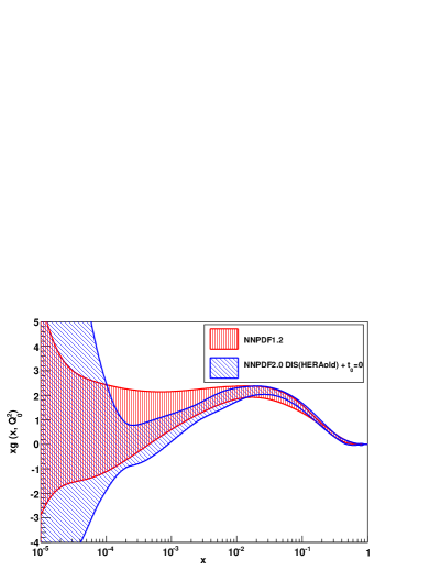

   

   

   

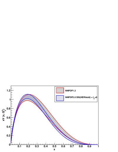
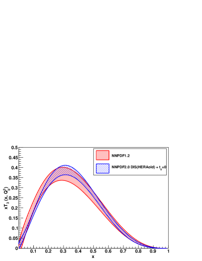
   Figure 24: Comparison between PDFs from the NNPDF1.2 fit and a fit to the same data but improved genetic algorithm and stopping (IGA) (the distances are shown in Fig. 23): small-$x$ gluon, valence and triplet (from left to right).

   The distance between NNPDF1.2 and this fit, which only differs from it because of the IGA, is shown in Fig. 23: the IGA affects essentially all PDFs by reducing their uncertainties, the two fits are always consistent at the 1-$\sigma$ level. The individual PDFs which are more affected are the triplet, the valence and the gluon at small-$x$, which are shown Fig. 24.

2. Impact of the treatment of normalization uncertainties.
   The IGA fit is now repeated by also using the improved $t_{0}$ method of Ref. [18] for the treatment of normalization uncertainties. This leads to a further small but not negligible improvement in fit quality, mostly due to the fixed–target DIS experiments which have largest normalization uncertainties. The distances between the two fits, which only differ in the treatment of normalizations, are shown in Fig. 25. The PDFs which are most affected are the small–$x$ singlet and gluon and the triplet. A more detailed discussion of the impact of the treatment of normalization uncertainties on fits to the NNPDF1.2 dataset was presented in Ref. [18] and will not be repeated here.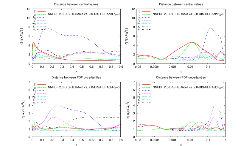

   

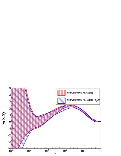
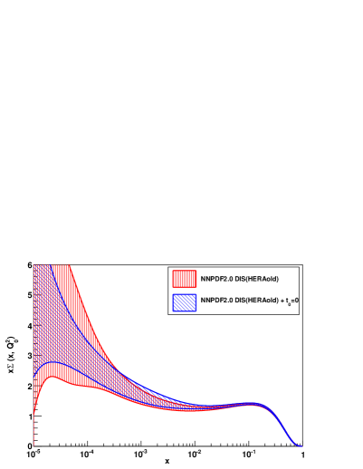
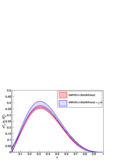
   Figure 25: Distance between the IGA fit of Fig. 23 and a fit with improved treatment of normalization uncertainties (IGA+$t_{0}$).

   

   

   

   Figure 26: Comparison between PDFs from the IGA fit of Fig. 23 and a fit with improved treatment of normalization uncertainties (IGA+$t_{0}$) (the distances are shown in Fig. 25): small-$x$ gluon, small $x$ singlet and triplet (from left to right).

3. Impact of the combined HERA-I data.
   The previous IGA+$t_{0}$ fit is now repeated replacing the ZEUS and H1 data with the new combined HERA-I dataset of Ref. [12]. This fit is now identical to the NNPDF2.0 fit, but with only DIS data (i.e. no hadronic data) included (2.0-DIS). The inclusion of the very precise HERA-I data leads to a slight deterioration of fit quality, which remains however still better than that of NNPDF1.2. This deterioration is concentrated in the HERA data themselves, with the quality of the fit to all other data unchanged. This suggests good consistency of the HERA and fixed target data, but with the accuracy of the combined HERA-I data now exceeding the accuracy of the theory used to describe them in NNPDF2.0: specifically, the lack of inclusion of charm mass corrections, but also possibly deviations from NLO DGLAP at small $x$ [66], or possible evidence for NNLO corrections at larger $x$. A particularly interesting aspect of this fit is that the quality of the fit to Drell-Yan data (not fitted), which was poor in all previous fits, improves considerably, especially for the $W$ asymmetry. This suggests that the accuracy of the charged–current data in the HERA-I combined set is now sufficient to provide some handle on the flavour decomposition of the sea at large $x$ which is only weakly constrained by neutral current DIS data, and strongly constrained by DY data.

   The distances between these fits is shown in Fig. 27: the impact of the combined HERA data is a moderate but generalized improvement in accuracy at small $x$. The effect on the singlet and the gluon at small-$x$ is shown in Fig. 28. The sizable error reduction in the small $x$ singlet is specially interesting.

   

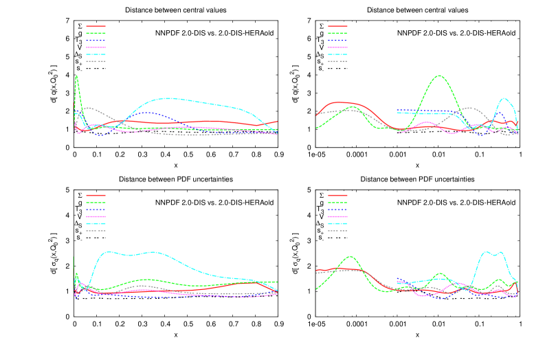
   Figure 27: Distance between the IGA+$t_{0}$ fit of Fig. 25 and a fit in which the separate H1 and ZEUS data are replaced by the combined HERA-I DIS data (NNPDF2.0 DIS).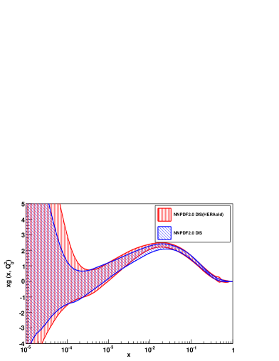

   

   

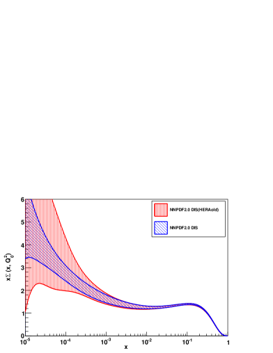
   Figure 28: Comparison between PDFs from IGA+$t_{0}$ fit of Fig. 25 and a fit in which the separate H1 and ZEUS data are replaced by the combined HERA-I DIS data (NNPDF2.0 DIS) (the distances are shown in Fig. 27): small-$x$ gluon and small $x$ singlet (from left to right).

4. Impact of jet data.
   The addition of jet data to the 2.0-DIS fit leaves the quality of the global fit unchanged. This demonstrates the perfect compatibility of jet data with DIS data: in fact, the quality of the fit to jet data was quite good even in all previous fits, in which they were not included in the fitted dataset. The distance between the 2.0-DIS and 2.0-DIS+JET fits, displayed in Fig. 29, shows that these data affect almost only the gluon, as one would expect [50], leading to a better determination of it at medium and large $x$. This is shown in Fig. 30, where the gluons of 2.0-DIS and 2.0-DIS+JET are compared.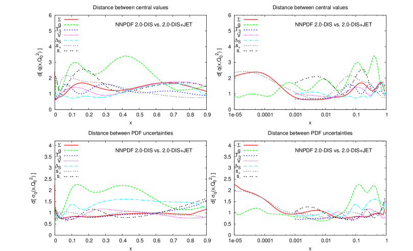

   

   Figure 29: Distance between the NNPDF2.0 DIS fit of Fig. 27 and a fit in which jet data are also included (NNPDF2.0 DIS+JET).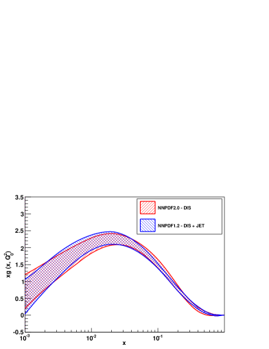

   

   

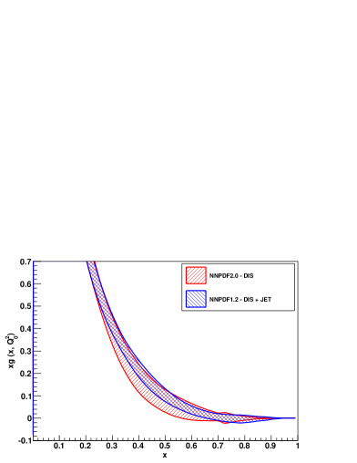
   Figure 30: Comparison between PDFs from NNPDF2.0 DIS fit of Fig. 27 and a fit in which jet data are also included (NNPDF2.0 DIS+JET) (the distances are shown in Fig. 29): the gluon at small and large $x$ (from left to right).

5. Impact of Drell-Yan data.
   The addition of Drell-Yan data to the 2.0-DIS+JET fit leaves the quality of the global fit unchanged. Taken together with the previous comparison of the 2.0-DIS and 2.0-DIS+JET data, this shows that DIS data and hadronic data are fully compatible, and furthermore the two classes of hadronic data included here, DY and inclusive jets, are compatible with each other. Minor incompatibilities only appear within each dataset (typically due to some subset of data points or, in the case of Drell-Yan to the CDF W asymmetry and Z rapidity distribution data). However, the quality of the fit to Drell-Yan data was generally poor when they were not included in the fit, due to the fact that they are sensitive to the separation of individual flavours at large $x$ which is only very weakly constrained by other data.

   The distances between the 2.0-DIS+JET and the full NNPDF2.0 fits, displayed in Fig. 31, show the sizable impact of the Drell-Yan data on all valence–like PDF combinations at medium and large-$x$: the triplet, the valence, the sea asymmetry and the strangeness asymmetry. The significant improvement in accuracy on all these PDFs is apparent in Fig. 30. The remarkable improvement in the accuracy of the determination of the strangeness asymmetry $s^{-}(x)$ will turn out to have relevant phenomenological implications for the so–called NuTeV anomaly, as we discuss in Sect. 6.

   

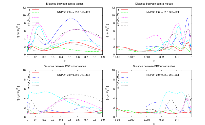
   Figure 31: Distance between the NNPDF2.0 DIS+JET fit of Fig. 29 and the reference NNPDF2.0 fit (Drell-Yan data also included).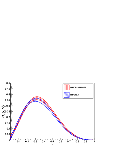

   

   

   

   

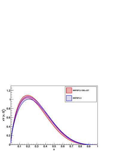
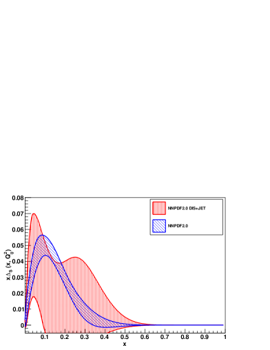
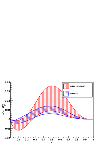
   Figure 32: Comparison between PDFs the NNPDF2.0 DIS+JET fit of Fig. 29 and the reference NNPDF2.0 fit (Drell-Yan data also included) (the distances are shown in Fig. 31): triplet, valence, sea asymmetry and strange valence (from left to right and from top to bottom).

Finally, we have produced two further PDF sets: one with the full NPDF2.0 dataset, but with HERA-I combined DIS data replaced by the previous separate H1 and ZEUS data; and the other with DIS+DY data only. In both cases, we see that the impact of the new data is independent of the dataset to which they are added: so for instance the improvement in accuracy in the valence sector due to DY data is independent of their being added to a dataset that does or does not contain jet data.

The main conclusion of this analysis is that we see no sign of tension between datasets. To understand this, consider what would happen if, say, jet data were incompatible with Drell-Yan data: then, we should see a daterioration of the quality of the fit to Drell-Yan when jets are included, and also we should see that the impact of jet data is bigger when Drell-Yan data are not included and more moderate when they are included. None of these effects is observed, for any of the combinations that have been tried here. Deterioration of the fit quality to each individual data set upon global fitting has been discussed in detailed in Ref. [65]: whereas small data incompatibilities may only be revealed by the more sensitive method used in this reference, we see no evidence for the sizable incompatibilties found there.

5.5 Positivity constraints

As discussed in Sect. 4, positivity of physical observables has been imposed, in particular for the longitudinal structure function $F_{L}(x,Q^{2})$ and for the dimuon cross section through a Lagrange multiplier Eq. (54). In order to assess quantitatively the effect of the positivity constraints, we have repeated the NNPDF2.0 parton determination without imposing positivity, i.e. setting $\lambda_{\rm pos}=0$ in Eq. (54).

In Fig. 33 PDFs with uncertainties determined as 68% confidence levels with and without positivity constraints are compared. As discussed in Sect. 5.3, it is important to perform the comparison with uncertainties determined as confidence levels rather than standard deviations, because imposing positivity can lead to deviations from gaussian behaviour. Clearly positivity of $F_{L}(x,Q^{2})$ leads to substantial uncertainty reduction in the small-$x$ gluon. Note that there is nevertheless a kinematic region in which the gluon goes negative by a small amount, though $F_{L}$ remains positive. Also, removing positivity of the dimuon cross section would lead to a much softer strange sea at small-$x$ with rather larger uncertainties. This in turn leads to a softer small-$x$ singlet, also with larger uncertainties. This is due to the fact that below $x\mathrel{\hbox to0.0pt{\lower 4.0pt\hbox{\hskip 1.0pt$\sim$}\hss}\raise 1.0pt\hbox{$<$}}0.01$, where no neutrino data are available, positivity is the only constraint on the total strangeness $s^{+}$.

Finally, it is interesting to observe that positivity also has the effect of stabilizing the replica sample: indeed, the 68% confidence levels computed without positivity display some visible fluctuations which would only be smoothened out by using a significantly wider replica sample. These fluctuations are absent when positivity is imposed, meaning that such wide fluctuations in individual replicas are removed by the constraint.

Figure 33: NNPDF2.0 PDFs with and without positivity constraints: singlet, gluon and total strangeness at small $x$ and total strangeness at large $x$. All uncertainty bands are determined as 68% confidence levels. PDFs not shown here are not affected by the positivity constraints.

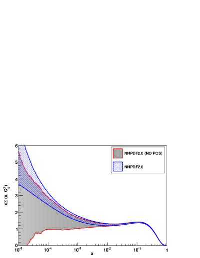
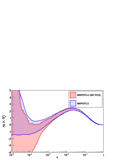
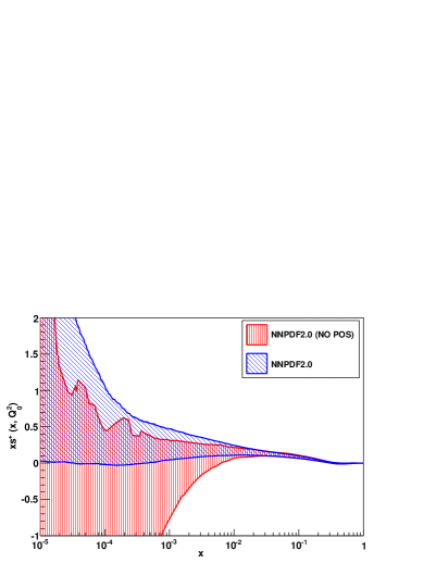
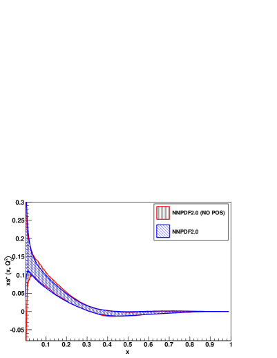
5.6 Dependence on $\alpha_{s}$

The central NNPDF2.0 fit has been performed with $\alpha_{s}(M_{Z})=0.119$ in order to ease comparison with the previous NNPDF1.0 and NNPDF1.2 fits, even though the current [67] PDG average is $\alpha_{s}(M_{Z})=0.118\pm 0.002$. In order to study the dependence of our results on this choice, we have repeated the fit with $\alpha_{s}$ varied by one and two standard deviations about this value, i.e. we have produced PDF sets with $\alpha_{s}(M_{Z})=0.115,\;0.117,\;0.121$ and $0.123$.

In the previous NNPDF1.0 and NNPDF1.2 parton sets the dependence of PDFs on $\alpha_{s}$ was found [4, 68, 69, 70] to be noticeable but weak: when $\alpha_{s}$ was varied by $\Delta\alpha_{s}=\pm 0.002$ most PDFs were found to be statistically indistinguishable from those obtained with $\alpha_{s}$ fixed to its central value (i.e. to be at a distance $d\approx 1$ from them). The gluon (and to a lesser extent the singlet PDF) was found to change in a statistically significant way, but still within its uncertainty band when $\alpha_{s}$ was varied in this range.

The dependence of NNPDF2.0 PDFs on $\alpha_{s}$ is shown in Fig. 34, where the ratio of the four $\alpha_{s}$ PDF sets to the central set are shown for all PDFs except the total strangeness $s^{+}$ which is found not to vary significantly. Clearly, all PDFs are still within the central uncertainty band when $\Delta\alpha_{s}=\pm 0.002$. However, there appears to be now somewhat greater sensitivity to $\alpha_{s}$. Firstly, now not only the gluon but also the triplet, singlet and valence, when $\alpha_{s}$ is varied in the range $\Delta\alpha_{s}=\pm 0.002$, move close to the edge of the one–$\sigma$ range for the central PDF. This corresponds to a distance $d\approx 7$, well above the threshold of statistical significance, and even for the gluon it is a somewhat larger variation than observed in NNPDF1.2. Furthermore, the triplet, which as discussed in Sect. 5.2 is now determined very accurately, appears to be as sensitive as the gluon to the value of $\alpha_{s}$. The increased sensitivity of quark distributions to the value of $\alpha_{s}$ is likely a consequence of the inclusion of Drell-Yan data, which undergo large NLO corrections and are thus sensitive to $\alpha_{s}$.

This increased sensitivity with respect to $\alpha_{s}$ suggests that the strong coupling could be determined from the global PDF analysis with competitive accuracy, following a procedure similar to that used to obtain the accurate determination of the CKM matrix element $|V_{\rm cs}|$ of Ref. [6].

Figure 34: Ratios of PDFs with $\alpha_{s}$ varied in the range $0.115\leq\alpha_{s}\leq 0.123$ to the central NNPDF2.0 determination, compared to the PDF uncertainty band: the singlet at small and large $x$, the gluon at small and large $x$ and the triplet, valence, sea asymmetry and strange valence (from top to bottom).

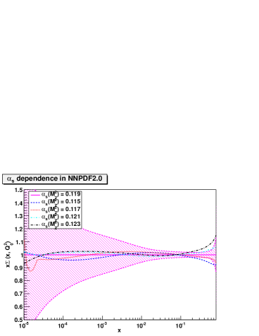
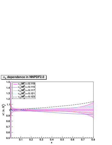
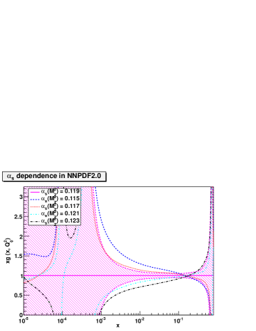
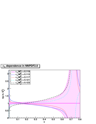
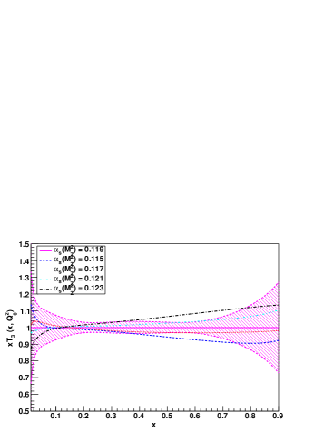
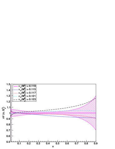
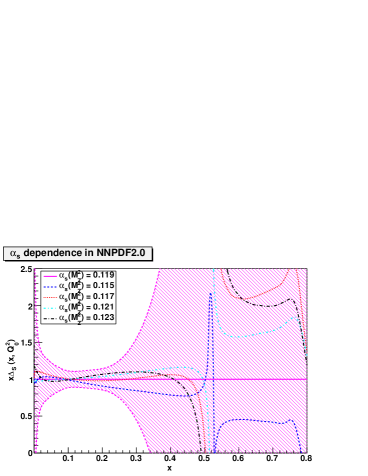
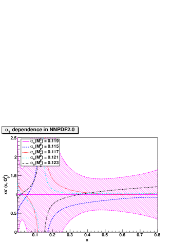
6 Phenomenological implications

A full phenomenological study of the implications of NNPDF2.0 PDFs is beyond the scope of this paper. In this section we present some preliminary investigations: we compare to the experimental data which has been included in the fit, then we discuss the implications for the proton strangeness and in particular to the NuTeV anomaly, and finally we present predictions for some LHC standard candles.

6.1 Comparison to experimental data

The general quality of predictions obtained using NNPDF2.0 PDFs for the observables which have been included in the fits has already been summarized in Table 10 and Fig. 12. A direct comparison of the data with theoretical predictions for some of these observables are shown in Fig. 35 (DIS and Drell-Yan) and Fig. 36 (inclusive jets).

Figure 35: Comparison between data and NLO predictions obtained using NNPDF1.0, NNPDF1.2 and NNPDF2.0 PDFs, for several DIS and Drell–Yan observables included in the NNPDF2.0 fit. From top to bottom and from left to right: the $F_{2}^{p}$ structure function and the $F_{2}^{d}/F_{2}^{p}$ (NMC), the inclusive neutrino cross-section (CHORUS), the Drell–Yan rapidity distribution (E866p), the $W-$asymmetry (CDF) and the Drell–Yan p/d ratio (E866). For the purposes of this plot only, experimental statistical and systematic uncertainties have been added in quadrature.

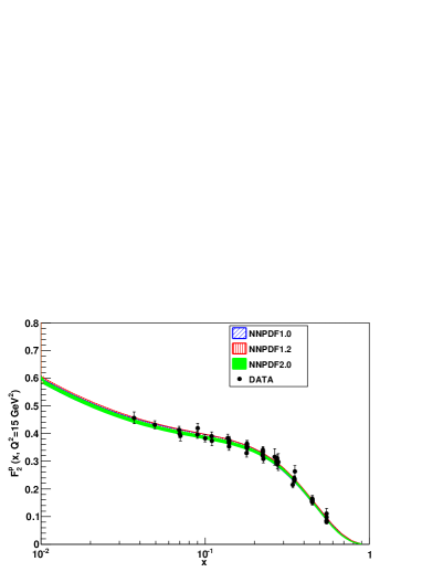
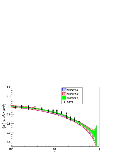
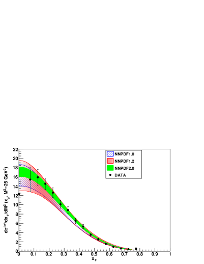
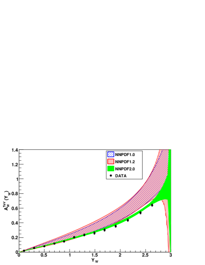
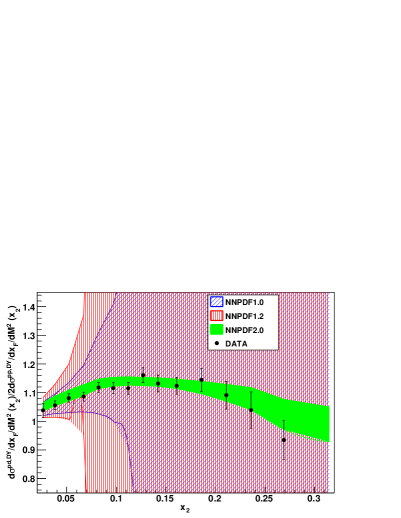
In Drell-Yan observables, the improvement in accuracy of the prediction when going from NNPDF1.2 to NNPDF2.0 is apparent: in particular, the sea asymmetry, virtually unconstrained from DIS, is now very well constrained by the E866 ratio data. Also the uncertainty reduction in the $W$-asymmetry measurement shows the increase in the precision of the determination of the quark decomposition in NNPDF2.0. In jet data, the excellent agreement between data and theory seen from the $\chi^{2}$ of Tab. 10 is seen to hold through the whole kinematical range for all bins in transverse momentum and rapidity.

Figure 36: Comparison between data and NLO predictions obtained using NNPDF2.0 PDFs, for inclusive jet production from D0 and CDF Run II. Data points are ordered in rapidity and in transverse momentum from left to right. Experimental statistical and systematic uncertainties have been added in quadrature for this plot. The NLO theoretical prediction has been obtained using the FastNLO code.

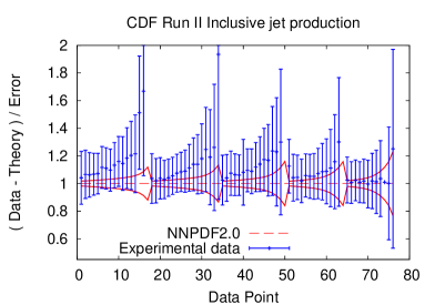
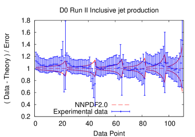
6.2 The proton strangeness revisited

In Ref. [6] a detailed study of the strangeness content in the proton was performed, with particular emphasis on the precision determination of electroweak parameters. The addition of fixed–target Drell–Yan data in the NNPDF2.0 PDF determination, together with other improvements in the fit that have been discussed in Sect. 5.4, leads to significantly stricter constraints on the shape of the strange distributions $s^{\pm}(x)$ PDFs, as shown in Figs. 13-14: while remaining consistent with the NNPDF1.2 result, the new determination of $s^{+}$ and especially $s^{-}$ at large $x$ have a much reduced uncertainty.

Indeed, the strange momentum fraction $K_{S}={{S^{+}}\over{U^{+}+D^{+}}}$ and strangeness asymmetry $R_{S}={{2S^{-}}\over{U^{-}+D^{-}}}$ [6] at $Q^{2}=20$ GeV² are

$$K_{S} = \begin{cases}0.71{{}^{+0.19}_{-0.31}}^{\rm stat}\pm 0.26^{\rm syst}&\qquad({\rm NNPDF1.2})\\ 0.503\pm 0.075^{\rm stat};&\qquad({\rm NNPDF2.0})\end{cases}$$ (59)

$$R_{S} = \begin{cases}0.006\pm 0.045^{\rm stat}\pm 0.010^{\rm syst}&({\rm NNPDF1.2})\\ 0.019\pm 0.008^{\rm stat}&({\rm NNPDF2.0}),\end{cases}$$ (60)

i.e. the PDF uncertainty on $K_{S}$ is reduced by more than a factor two, while that on $R_{S}$ is reduced by a factor 5, with all results consistent within uncertainties. We have made no attempt to provide a new determination of systematic and theoretical uncertainties on $R_{S}$, which are now comparable to the reduced statistical uncertainties, but they should be similar to those determined in Ref. [6] and quoted in Eqs. (59-60).

Figure 37: Distribution of $K_{S}$ at $Q^{2}=20$ GeV² computed from the reference set of $N_{\rm rep}=1000$ NNPDF2.0 PDF replicas. The central region corresponds to the 68% confidence interval, $K_{S}\left(Q^{2}=20\,{\rm GeV}^{2}\right)=0.503\pm 0.075~{}({\rm stat})$, which coincides with the 1–$\sigma$ interval Eq. 59).

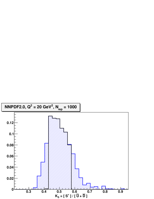
The distribution of $K_{S}$ values for 1000 NNPDF2.0 replicas is shown in Fig. 37: in comparison to the analogous plot in Ref. [6] the narrower distribution which we now get is closer to gaussian and indeed, unlike in Ref. [6], we now find no difference between the 68% confidence level and (symmetric) one–$\sigma$ intervals.

Figure 38: Determination of the Weinberg angle from the uncorrected NuTeV data [19], with $\left[S^{-}\right]$ correction using NNPDF1.2 (Eq. (60)) and NNPDF2.0 (Eq. (60)) results, and from a global electroweak fit [71]. Note that that statistical uncertainties only are included in the NNPDF2.0 correction.

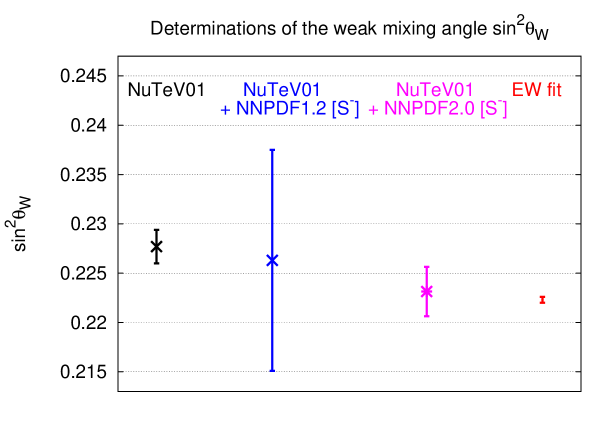
The implication of the accurate determination Eq. (60) of the strangeness asymmetry $R_{S}$ for the so–called NuTeV anomaly [20] are striking: in Fig. 38 we compare the NuTeV determination of the Weinberg angle [19], uncorrected or corrected for strangeness asymmetry as discussed in Ref. [6], using the values of $R_{S}$ Eqs. (60), and the result of a global electroweak fit [71]. The two corrected values, unlike the uncorrected NuTeV value, are in perfect agreement with the electroweak fit and with each other. However, while the uncertainty on the Weinberg angle with NNPDF1.2 correction was considerably larger, the uncertainty after NNPDF2.0 correction is comparable to that on the uncorrected value. Indeed, Eq. (60) provide a 2–$\sigma$ evidence for a non-zero and positive strangeness asymmetry in the nucleon. While such an asymmetry was previously advocated as a possible explanation of the NuTeV anomaly [20], evidence for it [72, 73, 19, 11] was so far inconclusive, and it is being established here for the first time.

6.3 Parton luminosities

In order to highlight the impact of parton distributions at LHC the parton–parton luminosities (also called partonic fluxes) are relevant [74, 75]; of particular interest are the sizes of PDF uncertainties in parton luminosities from different PDF sets.

Figure 39: Parton–parton luminosities Eq. (61) in the various partonic channels, computed from the NNPDF2.0 set at the LHC for $\sqrt{s}=$ 14 TeV (above) and ratio of results for 7 TeV and 14 TeV (below).

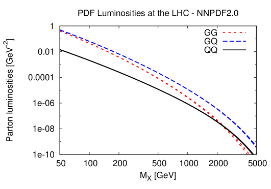
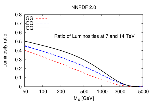
We can define three relevant combinations of PDF luminosities for the production of a massive object with mass $M_{X}$ in hadronic collisions as follows:

$$\Phi_{gg}\left(M_{X}^{2}\right) = {{1}\over{s}}\int_{\tau}^{1}{{dx_{1}}\over{x_{1}}}g\left(x_{1},M_{X}^{2}\right)g\left(\tau/x_{1},M_{X}^{2}\right)\ ,$$

$$\Phi_{gq}\left(M_{X}^{2}\right) = {{1}\over{s}}\int_{\tau}^{1}{{dx_{1}}\over{x_{1}}}\left[g\left(x_{1},M_{X}^{2}\right)\Sigma\left(\tau/x_{1},M_{X}^{2}\right)+(1\to 2)\right]\ ,$$ (61)

$$\Phi_{qq}\left(M_{X}^{2}\right) = {{1}\over{s}}\int_{\tau}^{1}{{dx_{1}}\over{x_{1}}}\sum_{i=1}^{N_{f}}\left[q_{i}\left(x_{1},M_{X}^{2}\right)\bar{q}_{i}\left(\tau/x_{1},M_{X}^{2}\right)+(1\to 2)\right]\ ,$$

with $\tau\equiv M_{X}^{2}/s$ and $\sqrt{s}$ the center of mass energy of the hadronic collision.

In Fig. 39 we show the various partonic luminosities Eq. (61) at the LHC as computed with the NNPDF2.0 set. It is clear that at low masses the GG and GQ channels are both important, while at large masses the GQ channel dominates. Also in Fig. 39 we show the ratio of partonic luminosities between LHC 14 TeV and 7 TeV. While at small masses the loss in partonic luminosity is roughly a factor two, it can be as large as a factor ten or more at large masses. The gluon-gluon luminosity is the channel which suffers the greatest reduction.

Figure 40: Relative PDF uncertainties on parton–parton luminosities Eq. (61) for the NNPDF2.0, CTEQ6.6 and MSTW2008 PDF sets, as function of the mass of the produced heavy object $M_{X}$ at the LHC for 14 TeV (left) and 7 TeV (right). From top to bottom, the gluon-gluon luminosity, the gluon-quark luminosity and the quark-quark luminosity are shown.

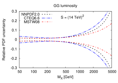
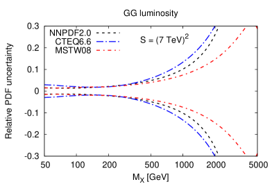
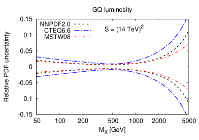
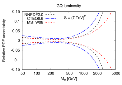
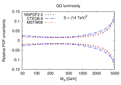
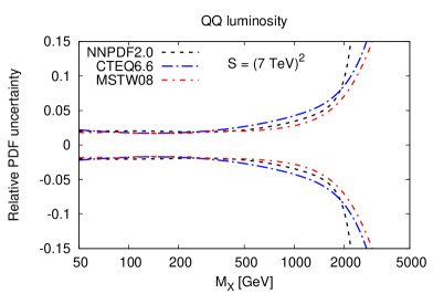
Turning now to the uncertainties on parton luminosities due to PDFs, in Fig. 40 we compare the relative PDF uncertainties (normalized to the respective central set) in various channels of PDF luminosity for the NNPDF2.0, CTEQ6.6 and MSTW08 sets. In the GG channel, all PDF sets agree in the central mass region, and NNPDF2.0 is close to MSTW08 in general. In the QQ channel all PDF sets yield very similar uncertainties at small and medium masses. It is also clear from Fig. 40 that at 7 TeV the restricted $x$-range of the partons leads to sizably larger PDF uncertainties at large values of $M_{X}$.

6.4 LHC standard candles

The total cross sections at the LHC with $\sqrt{s}=14$ TeV for $W$, $Z$, $H$ and $t\bar{t}$ production computed at NLO with MCFM [76, 77, 78, 79] and NNPDF2.0, NNPDF1.2., CTEQ6.6, and MSTW08 PDFs are compared in Table 12 and Fig. 41. Values obtained using NNPDF2.0 are in excellent agreement with those from NNPDF1.2, with significantly smaller uncertainties. The predictions from previous NNPDF sets were discussed in [6].

	$\sigma(W^{+}){\rm Br}\left(W^{+}\to l^{+}\nu_{l}\right)\,$	$\sigma(W^{-}){\rm Br}\left(W^{-}\to l^{+}\nu_{l}\right)\,$	$\sigma(Z^{0}){\rm Br}\left(Z^{0}\to l^{+}l^{-}\right)\,$
NNPDF1.2	$11.99\pm 0.34$ nb	$8.47\pm 0.21$ nb	$1.94\pm 0.04$ nb
NNPDF2.0	$11.57\pm 0.19$ nb	$8.52\pm 0.14$ nb	$1.93\pm 0.03$ nb
CTEQ6.6	$12.41\pm 0.28$ nb	$9.11\pm 0.22$ nb	$2.07\pm 0.05$ nb
MSTW08	$12.03\pm 0.22$ nb	$9.09\pm 0.17$ nb	$2.03\pm 0.04$ nb

	$\sigma(t\bar{t})$	$\sigma(H,m_{H}=120\,{\rm GeV})$
NNPDF1.2	$901\pm 21$ pb	$36.6\pm 1.2$ pb
NNPDF2.0	$913\pm 17$ pb	$37.3\pm 0.4$ pb
CTEQ6.6	$844\pm 17$ pb	$36.3\pm 0.9$ pb
MSTW08	$905\pm 18$ pb	$38.4\pm 0.5$ pb

Table 12: Cross sections for W, Z, $t\bar{t}$ and Higgs production at the LHC at $\sqrt{s}=14$ TeV. All quantities have been computed at NLO using MCFM [76, 77, 78, 79] with default settings for the NNPDF1.2, NNPDF2.0, CTEQ6.6 and MSTW08 PDF sets. All uncertainties shown are one–sigma. The Higgs cross section corresponds to the gluon-gluon fusion production channel.

It was already observed in Ref. [4] that NNPDF results for W and Z production agree with those of CTEQ6.1, but undershoot the CTEQ6.5 and CTEQ6.6 predictions by more than 5%. The main difference between CTEQ6.5/CTEQ6.6 and CTEQ6.1 is that charm mass effects are included in the former pair of fits, but not in the latter, and are also not included in all available NNPDF fits. This suggests that charm mass effects be responsible for the discrepancy between the CTEQ6.6 and NNPDF predictions for $W$ and $Z$ cross sections. It should be noticed however that NNPDF1.0 results do agree [4] with MRST01 [80], and do not agree with MSTW08 (as it is clear from Table 12) despite the fact that charm mass effects are included both in MRST01 and MSTW08. The pattern for Higgs and $t\bar{t}$ production is even less clear, with NNPDF in good agreement with MSTW08 but not CTEQ6.6 for the former, and in good agreement with CTEQ6.6 but not MSTW08 for the latter.

Figure 41: Graphical comparison of the cross sections from Table 12.

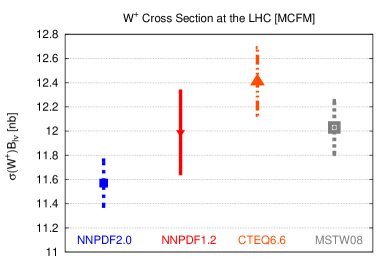
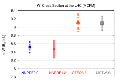
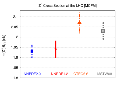
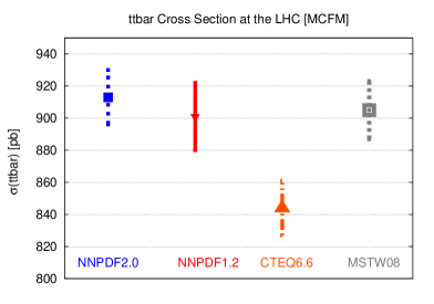
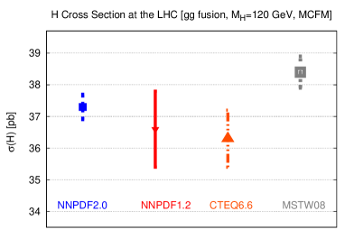
Note however that most of these cross sections are quite sensitive to the value of $\alpha_{s}$, and some of them extremely sensitive: for example, the contribution to the Higgs cross section from gluon-gluon fusion varies by about 5% when $\alpha_{s}$ is varied by 2%. The results shown in Table 12 and Fig. 41 have been obtained with the default settings of MCFM, and in particular with the value of $\alpha_{s}$ corresponding to each group’s central parton fit, namely $\alpha_{s}(M_{Z})=0.118$ for CTEQ6.6 and $\alpha_{s}(M_{Z})=0.120$ for MSTW08 (and $\alpha_{s}(M_{Z})=0.119$ for NNPDF2.0). Hence, benchmarking of these cross sections with the same value of all parameters including $\alpha_{s}$ should be performed before conclusions can be drawn.

It should finally be noticed that some approximations used in the MSTW08 and CTEQ6.6 PDF determinations but not by NNPDF could have an impact on these observables, such as the use of $K$–factors in fitting Drell-Yan data by both MSTW and CTEQ, the use of a restrictive small $x$ parametrization of the gluon by CTEQ, and the use of very restrictive parametrizations of strangeness by both MSTW and CTEQ. In summary, while the lack of inclusion of heavy quark terms may be responsible for some of the discrepancies observed in Table 12 and Fig. 41 it cannot be the only explanation (it cannot account for cases in which NNPDF agrees with CTEQ but not MSTW or conversely). The issue should be re-examined after the inclusion of heavy quark mass effects in NNPDF, ideally within a systematic benchmarking of parton distributions.

7 Conclusions and outlook

The NNPDF2.0 parton determination is the first global parton determination based on NNPDF methodology, and it is also the first global parton determination in which NLO QCD is used consistently throughout, without resorting to the $K$–factor approximation. We have seen that the NNPDF methodology can accommodate a complex combination of DIS and hadronic datasets without any particular difficulties: in fact, the only bottleneck in the implementation of the NNPDF2.0 global fit has been computational, requiring the development of the FastKernel method discussed in Sect. 3 in order for DGLAP evolution and the computation of physical observables to be fast enough.

In previous NNPDF work it was shown that NNPDF parton determinations behave in a statistically consistent way upon the subsequent inclusion of new data, without any adjustment being required as the new data are included, and with uncertainties decreasing upon the addition of new information, or at most remaining constant when inconsistent data are added. Here we have seen that this remains true when hadronic and deep–inelastic data are combined. In fact, we have found complete consistency between DIS and hadronic data, with some hadronic data (jets) being reasonably well predicted by the DIS fit and leading to small improvements, and other hadronic data (Drell-Yan) introducing new information which allows a quantitative determination of some PDF combinations that were determined with moderate or poor accuracy by DIS data, such as the light quark sea asymmetry.

Progress has been made recently towards the inclusion of heavy quark mass effects in the NNPDF framework [81] and in the benchmarking of different approaches for the inclusion of heavy quark mass effects [70]. Once these are included in a global NNPDF fit accurate and reliable NLO phenomenology at the LHC will be possible.

 

The NNPDF2.0 PDFs (sets of $N_{\rm rep}=100$ and 1000 replicas), as well as several of the sets based on reduced or different datasets discussed in Sect. 5.4 (old HERA-I data, DIS only, DIS+JET only, DIS+DY only, sets of $N_{\rm rep}=100$ replicas), and also sets determined using all values of $0.114\leq\alpha_{s}(M_{Z})0.124$ in steps of $\Delta\alpha_{s}(M_{Z})=0.001$ are available from the NNPDF web site,

http://sophia.ecm.ub.es/nnpdf .

They are also available through the LHAPDF interface [8].

Acknowledgments

We would like to thank J. C. Webb for help with the E866 data, E. Halkiadakis for help with the CDF direct $W$ asymmetry production data, H. Schellman for assistance with D0 electroweak data, M. Martínez-Pérez for discussions about Run II inclusive jet production data and A. Cooper-Sarkar for discussions concerning the combined HERA-I data. We also thank A. Accardi for information on the CTEQ6.X fits. We are especially grateful to A. Vicini and G. Ridolfi for providing us with the Drell-Yan code used in the FastKernel code benchmarking. We acknowledge extensive discussions and correspondence with members of the PDF4LHC workshop, in particular A. de Roeck, A. Glazov, J. Huston, R. McNulty, P. Nadolsky, F. Olness, and especially J. Pumplin and R. Thorne whom we thank for raising issues related to the proper learning of neural networks. This work was partly supported by a Spanish MEC FIS2007-60350 grant and by the European network HEPTOOLS under contract MRTN-CT-2006-035505. L.D.D. is funded by an STFC Advanced Fellowship and M.U. by a SUPA graduate studentship. We would like to acknowledge the use of the computing resources provided by the Black Forest Grid Initiative in Freiburg and by the Edinburgh Compute and Data Facility (ECDF) (http://www.ecdf.ed.ac.uk/). The ECDF is partially supported by the eDIKT initiative (http://www.edikt.org.uk).

Appendix A Distances between PDFs: definition and meaning

Given two sets of $N^{(1)}_{\mathrm{rep}}$ and $N^{(2)}_{\mathrm{rep}}$ replicas, one is often interested in knowing whether they correspond to different instances of the same underlying probability distribution, or whether instead they come from different underlying distributions. Of course, for finite $N^{(i)}_{\mathrm{rep}}$ this question can only be answered in a statistical sense. To this purpose, we define the square distance between two estimators based on the given samples as the square difference between the estimators divided by its expectation value, i.e. divided by the corresponding standard deviation. By construction, the expectation value of the distance is one.

The following cases are of particular interest:

• Expected value
  

  Given a set of $N^{(k)}_{\mathrm{rep}}$ replicas $q^{(k)}_{i}$ of some quantity $q$, the estimator for the expected (true) value of $q$ is the mean

  $$\langle q^{(k)}\rangle_{(i)}={{1}\over{N^{(i)}_{\mathrm{rep}}}}\sum_{i=1}^{N^{(i)}_{\mathrm{rep}}}q^{(k)}_{i}.$$ (62)

  The square distance between the two estimates of the expected value obtained from sets $q^{(1)}_{i}$, $q^{(2)}_{i}$ is then

  $$d^{2}\left(\langle q^{(1)}\rangle,\langle q^{(2)}\rangle\right)={{\left(\langle q^{(1)}\rangle_{(1)}-\langle q^{(2)}\rangle_{(2)}\right)^{2}}\over{\sigma^{2}_{(1)}[\langle q^{(1)}\rangle]+\sigma^{2}_{(2)}[\langle q^{(2)}\rangle]}}$$ (63)

  where the variance of the mean is given by

  $$\sigma^{2}_{(i)}[\langle q^{(i)}\rangle]={{1}\over{N^{(i)}_{\mathrm{rep}}}}\sigma^{2}_{(i)}[q^{(i)}]$$ (64)

  in terms of the variance $\sigma^{2}_{(i)}[q^{(i)}]$ of the variables $q^{(i)}$ (which a priori could come from two distinct probability distributions). We estimate the variance of the mean from the variance of the replica sample as

  $$\sigma^{2}_{(i)}[q^{(i)}]={{1}\over{N^{(i)}_{\mathrm{rep}}-1}}\sum_{k=1}^{N^{(i)}_{\mathrm{rep}}}\left(q^{(i)}_{k}-\langle q^{(i)}\rangle\right)^{2},$$ (65)

  with $\langle q^{(i)}\rangle$ given by Eq. (62).

• Uncertainty
  

  Given a set of $N^{(k)}_{\mathrm{rep}}$ replicas $q^{(k)}_{i}$ of some quantity $q$, the estimator for the square uncertainty of $q$ is the variance of the replica sample given by Eq. (65). The distance between the two estimates of the square uncertainty obtained from sets $q^{(1)}_{i}$, $q^{(2)}_{i}$ is then

  $$d^{2}(\sigma^{2}_{(1)},\sigma^{2}_{(2)})={{\left(\bar{\sigma}^{2}_{(1)}-\bar{\sigma}^{2}_{(2)}\right)^{2}}\over{\sigma^{2}_{(1)}[\bar{\sigma}^{2}_{(1)}]+\sigma^{2}_{(2)}[\bar{\sigma}^{2}_{(2)}]}}$$ (66)

  where for brevity we have defined

  $$\bar{\sigma}^{2}_{(i)}\equiv\sigma^{2}_{(i)}[q^{(i)}].$$ (67)

  The variances $\sigma^{2}_{(i)}[\bar{\sigma}^{2}_{(i)}]$ of the square uncertainties could also be estimated from the replica sample, by computing the variance from various subsets of the given replica sample, and then the variance of these resulting variances as the subset is varied; for finite number of replicas this may lead to loss of statistical accuracy. For simplicity here we use instead the expression [67]

  $$\sigma^{2}_{(i)}[\bar{\sigma}^{2}_{(i)}]={{1}\over{N_{\mathrm{rep}}^{(i)}}}\left[m_{4}[q^{(i)}]-{{N_{\mathrm{rep}}^{(i)}-3}\over{N_{\mathrm{rep}}^{(i)}-1}}\left(\bar{\sigma}^{2}_{(i)}\right)^{2}\right],$$ (68)

  where as above $\bar{\sigma}^{2}_{(i)}$ is estimated using Eq. (65), while the fourth moment $m_{4}$ of the probability distribution is estimated from the corresponding moment of the replica sample (which provides an estimate of it which is only asymptotically unbiased):

  $$m_{4}[q^{(i)}]={{1}\over{N^{(i)}_{\mathrm{rep}}}}\sum_{k=1}^{N^{(i)}_{\mathrm{rep}}}\left(q^{(i)}_{k}-\langle q^{(i)}\rangle\right)^{4}.$$ (69)

In practice, for small–sized replica samples the distances defined in Eq. (63) and Eq. (66) display sizable statistical fluctuations. In order to stabilize the result, all distances computed in this paper are determined as follows: we randomly pick $N^{(i)}_{\mathrm{rep}}/2$ out of the $N^{(i)}_{\mathrm{rep}}$ replicas for each of the two subsets. The computation of the square distance Eq. (63) or Eq. (66) is then repeated for $N_{\mathrm{part}}=100$ (randomly generated) choices of $N^{(i)}_{\mathrm{rep}}/2$ replicas, and the result is averaged: this is sufficient to bring the statistical fluctuations of the distance at the level of a few percent. The distances shown in Sect. 5 are the square root of this average, computed taking for $q^{(i)}$ the value of some PDF at fixed $x$ and $Q^{2}$ obtained from a given pair of fits. Through Sect. 5 the choice $Q^{2}=Q^{2}_{0}=2$ GeV² is always adopted.

The distance defined in this way measures whether the given samples do or do not come from the same underlying probability distribution, and in particular Eq. (63) and Eq. (66) test whether the two distributions from which the two samples are taken have respectively the same mean and the same standard deviation. By construction, the probability distribution for the distance coincides with the $\chi^{2}$ distribution with one degree of freedom, and thus it has mean $\langle d\rangle=1$, and $d\mathrel{\hbox to0.0pt{\lower 4.0pt\hbox{\hskip 1.0pt$\sim$}\hss}\raise 1.0pt\hbox{$<$}}2.3$ at 90% confidence level.

Note that asking whether two PDF determinations come from the same underlying distribution is much more restrictive than asking whether they are consistent within uncertainties. Consider for instance the case of a pair of PDF determinations, such that the dataset on which one of the two is based is a subset of the dataset of the other, and such that all data are consistent with each other. These two determinations will clearly not come from the same underlying distribution, because the distribution of PDFs obtained from the wider dataset will have smaller uncertainty. However, if the data are consistent they will remain nevertheless consistent within uncertainties.

In particular, the determination of moments of the underlying distribution becomes more precise as as the number of replicas is increased: e.g. the accuracy in determination of the expectation value scales as $1/\sqrt{N_{\mathrm{rep}}}$, compare Eq. (64), so if the underlying probability distributions are different the distance will grow as $\sqrt{N_{\mathrm{rep}}}$ in the large $N_{\mathrm{rep}}$ limit. In this limit (in which the central values of the underlying distribution are accurately estimated by mean over the replica sample) the distance between central values is given by the distance rescaled by $\sqrt{N_{\mathrm{rep}}}$: otherwise stated, if $N^{(1)}_{\mathrm{rep}}=N^{(2)}_{\mathrm{rep}}=N_{\mathrm{rep}}$, then

$$\delta(\sigma^{2}_{(1)},\sigma^{2}_{(2)})\equiv{{1}\over{\sqrt{N_{\mathrm{rep}}}}}d(\sigma^{2}_{(1)},\sigma^{2}_{(2)})$$ (70)

provides (in the large $N_{\mathrm{rep}}$) limit, the difference between central values in units of the standard deviation. It follows that because of the halving of the size of the sample required for averaging as discussed above, for all distances shown in Sect. 5, and computed with $N_{\mathrm{rep}}=100$ replicas, one sigma corresponds to $d=\sqrt{50}\approx 7$.

Appendix B Drell–Yan observables

We provide here the full expressions for Drell-Yan observables included into the NNPDF2.0 analysis (both virtual photon and vector boson production). We adopt the notations and conventions of Refs. [54, 55]. For explicit expression of the inclusive jet cross–sections, we can refer to the documentation of the FastNLO project from which we took the precomputed tables [16].

B.1 Rapidity and $x_{F}$ distributions

The leading order parton kinematics was given in Eq. (3). The rapidity distribution for the DY process can be then expressed at NLO as

$${{{\rm d}\sigma}\over{{\rm d}M^{2}{\rm d}y}}(M^{2},y) = {{4\pi\alpha^{2}}\over{9M^{2}s}}\sum_{i}e_{i}^{2}\int_{x_{1}^{0}}^{1}{\rm d}x_{1}\int_{x_{2}^{0}}^{1}{\rm d}x_{2}$$ (71)

$$\times\Bigg{\{}\left[D_{q\bar{q}}^{(0)}(x_{1},x_{2})+{{\alpha_{s}}\over{4\pi}}D_{q\bar{q}}^{(1)}\left(x_{1},x_{2},{{M^{2}}\over{\mu_{F}^{2}}}\right)\right]\Big{\{}q_{i}(x_{1},\mu_{F}^{2})\bar{q}_{i}(x_{2},\mu_{F}^{2})+\bar{q}_{i}(x_{1},\mu_{F}^{2})q_{i}(x_{2},\mu_{F}^{2})\Big{\}}$$

$$+\Bigg{[}{{\alpha_{s}}\over{4\pi}}D_{g\bar{q}}^{(1)}\left(x_{1},x_{2},{{M^{2}}\over{\mu_{F}^{2}}}\right)g(x_{1},\mu_{F}^{2})\left\{q_{i}(x_{2},\mu_{F}^{2})+\bar{q}_{i}(x_{2},\mu_{F}^{2})\right\}+(1\leftrightarrow 2)\Bigg{]}\Bigg{\}}\ .$$

The LO coefficient functions for this distribution are given by

$$D_{q\bar{q}}^{(0)}(x_{1},x_{2})=\delta(x_{1}-x_{1}^{0})\,\delta(x_{2}-x_{2}^{0});$$ (72)

the NLO contribution is explicitly given in Ref. [54].

For their practical implementation we exploited the following standard identities:

$${\rm Li}_{2}(x) = -\int_{0}^{x}dt{{\ln(1-t)}\over{t}}$$ (73)

$$\int_{x}^{1}dt{{f(t)}\over{(t-x)_{+}}} = \int_{x}^{1}dt{{f(t)-f(x)}\over{t-x}}$$ (74)

$$\int_{x}^{1}dtf(t)\left[{{\ln(1-x/t)}\over{t-x}}\right]_{+} = \int_{x}^{1}dt\left(f(t)-f(x)\right)\left[{{\ln(1-x/t)}\over{t-x}}\right]$$ (75)

$$\int_{x_{1}}^{1}dt_{1}\int_{x_{2}}^{1}dt_{2}{{f(t_{1},t_{2})}\over{\left[(t_{1}-x_{1})(t_{2}-x_{2})\right]_{+}}} =$$ (76)

$$\int_{x_{1}}^{1}dt_{1}\int_{x_{2}}^{1}dt_{2}{{f(t_{1},t_{2})-f(t_{1},x_{2})-f(x_{1},t_{2})+f(x_{1},x_{2})}\over{\left[(t_{1}-x_{1})(t_{2}-x_{2})\right]}}$$

Distributions in terms of Feynman $x_{F}$ are also frequently used: the leading order parton kinematics was given in Eq. (4). The Drell–Yan $x_{F}$ distribution of lepton pairs at NLO is given by

$${{{\rm d}^{2}\sigma}\over{{\rm d}M^{2}{\rm d}x_{F}}} = {{4\pi\alpha^{2}}\over{9M^{2}s}}\sum_{i}e_{i}^{2}\int_{x_{1}^{0}}^{1}{\rm d}x_{1}\int_{x_{2}^{0}}^{1}{\rm d}x_{2}$$ (77)

$$\times\Bigg{\{}\left[\widetilde{D}^{(0)}_{q\bar{q}}(x_{1},x_{2})+{{\alpha_{s}}\over{4\pi}}\widetilde{D}^{(1)}_{q\bar{q}}\left(x_{1},x_{2},{{M^{2}}\over{\mu_{F}^{2}}}\right)\right]\Big{\{}q_{i}(x_{1},\mu_{F}^{2})\bar{q}_{i}(x_{2},\mu_{F}^{2})+\bar{q}_{i}(x_{1},\mu_{F}^{2})q_{i}(x_{2},\mu_{F}^{2})\Big{\}}$$

$$+\Bigg{[}{{\alpha_{s}}\over{4\pi}}\widetilde{D}^{(1)}_{g\bar{q}}\left(x_{1},x_{2},{{M^{2}}\over{\mu_{F}^{2}}}\right)g(x_{1},\mu_{F}^{2})\left\{q_{i}(x_{2},\mu_{F}^{2})+\bar{q}_{i}(x_{2},\mu_{F}^{2})\right\}+(1\leftrightarrow 2)\Bigg{]}\Bigg{\}},$$

where the sum over $i$ runs over all $N_{f}$ quark flavours.

The LO coefficient function is given by

$$\widetilde{D}^{(0)}_{q\bar{q}}\left(x_{1},x_{2}\right)={{\delta(x_{1}-x_{1}^{0})\,\delta(x_{2}-x_{2}^{0})}\over{x_{1}^{0}+x_{2}^{0}}}.$$ (78)

The NLO contribution coming from $q\bar{q}$ annihilation is explicitly given in Ref. [55].

B.2 Vector boson production

For vector boson production at hadron colliders, the cross section is differential in a single variable $y$, the rapidity of the vector boson. The unpolarized vector boson production cross sections at NLO is

$${{{\rm d}\sigma}\over{{\rm d}y}} = {{\pi G_{F}M_{V}^{2}\sqrt{2}}\over{3s}}\sum_{i,j}c_{ij}\int_{x_{1}^{0}}^{1}{\rm d}x_{1}\int_{x_{2}^{0}}^{1}{\rm d}x_{2}$$ (79)

$$\times\Bigg{\{}\left[D_{q\bar{q}}^{(0)}(x_{1},x_{2},x_{1}^{0},x_{2}^{0})+{{\alpha_{s}}\over{4\pi}}D_{q\bar{q}}^{(1)}\left(x_{1},x_{2},x_{1}^{0},x_{2}^{0},{{M^{2}}\over{\mu_{F}^{2}}}\right)\right]$$

$$\times\Big{\{}q_{i}(x_{1},\mu_{F}^{2})\bar{q}_{j}(x_{2},\mu_{F}^{2})+\bar{q}_{i}(x_{1},\mu_{F}^{2})q_{j}(x_{2},\mu_{F}^{2})\Big{\}}$$

$$+{{\alpha_{s}}\over{4\pi}}D_{gq}^{(1)}\left(x_{1},x_{2},x_{1}^{0},x_{2}^{0},{{M^{2}}\over{\mu_{F}^{2}}}\right)g(x_{1},\mu_{F}^{2})\left\{q_{j}(x_{2},\mu_{F}^{2})+\bar{q}_{j}(x_{2},\mu_{F}^{2})\right\}$$

$$+{{\alpha_{s}}\over{4\pi}}D_{qg}^{(1)}\left(x_{1},x_{2},x_{1}^{0},x_{2}^{0},{{M^{2}}\over{\mu_{F}^{2}}}\right)\left\{q_{i}(x_{1},\mu_{F}^{2})+\bar{q}_{i}(x_{1},\mu_{F}^{2})\right\}g(x_{2},\mu_{F}^{2})\Bigg{\}}\;,$$

where $c_{ij}$ are the electroweak couplings defined in Eq. (10) The coefficient functions in Eq. (79) are identical to those in the Drell-Yan rapidity distribution Eq. (71).

Note that for proton–antiproton collisions (such as at the Tevatron) one of the two parton distributions refers to a proton and the other to an antiproton, i.e. in practice one should replace $q_{i}(x_{2})\to\bar{q}_{i}(x_{2})$ and conversely in the above expression. Similarly for proton-nucleus collisions, where isospin symmetry of the nucleus target should be taken into account.

References

- [1] S. Forte et al., JHEP 05 (2002) 062, hep-ph/0204232.
- [2] NNPDF, L. Del Debbio et al., JHEP 03 (2005) 080, hep-ph/0501067.
- [3] NNPDF, L. Del Debbio et al., JHEP 03 (2007) 039, hep-ph/0701127.
- [4] NNPDF, R.D. Ball et al., Nucl. Phys. B809 (2009) 1, 0808.1231.
- [5] NNPDF, J. Rojo et al., (2008), 0811.2288.
- [6] The NNPDF, R.D. Ball et al., Nucl. Phys. B823 (2009) 195, 0906.1958.
- [7] LHAPDF, http://projects.hepforge.org/lhapdf/.
- [8] D. Bourilkov, R.C. Group and M.R. Whalley, (2006), hep-ph/0605240.
- [9] M. Dittmar et al., (2009), 0901.2504.
- [10] P.M. Nadolsky et al., Phys. Rev. D78 (2008) 013004, 0802.0007.
- [11] A.D. Martin et al., Eur. Phys. J. C63 (2009) 189, 0901.0002.
- [12] H1 and ZEUS, A.F. D et al., (2009), 0911.0884.
- [13] S. Alekhin, K. Melnikov and F. Petriello, Phys. Rev. D74 (2006) 054033, hep-ph/0606237.
- [14] T. Carli, G.P. Salam and F. Siegert, (2005), hep-ph/0510324.
- [15] M. Dittmar et al., (2005), hep-ph/0511119.
- [16] T. Kluge, K. Rabbertz and M. Wobisch, (2006), hep-ph/0609285.
- [17] T. Carli et al., (2009), 0911.2985.
- [18] NNPDF, R.D. Ball et al., (2009), 0912.2276.
- [19] D. Mason et al., Phys. Rev. Lett. 99 (2007) 192001.
- [20] S. Davidson et al., JHEP 02 (2002) 037, hep-ph/0112302.
- [21] New Muon Collaboration, M. Arneodo et al., Nucl. Phys. B487 (1997) 3, hep-ex/9611022.
- [22] New Muon Collaboration, M. Arneodo et al., Nucl. Phys. B483 (1997) 3, hep-ph/9610231.
- [23] L.W. Whitlow et al., Phys. Lett. B282 (1992) 475.
- [24] BCDMS, A.C. Benvenuti et al., Phys. Lett. B223 (1989) 485.
- [25] CHORUS, G. Onengut et al., Phys. Lett. B632 (2006) 65.
- [26] H1, F.D. Aaron et al., Phys. Lett. B665 (2008) 139, 0805.2809.
- [27] NuTeV, M. Goncharov et al., Phys. Rev. D64 (2001) 112006, hep-ex/0102049.
- [28] D.A. Mason, FERMILAB-THESIS-2006-01.
- [29] ZEUS, S. Chekanov et al., (2009), 0901.2385.
- [30] ZEUS, S. Chekanov et al., (2008), 0812.4620.
- [31] G. Moreno et al., Phys. Rev. D43 (1991) 2815.
- [32] NuSea, J.C. Webb et al., (2003), hep-ex/0302019.
- [33] J.C. Webb, (2003), hep-ex/0301031.
- [34] FNAL E866/NuSea, R.S. Towell et al., Phys. Rev. D64 (2001) 052002, hep-ex/0103030.
- [35] CDF, T. Aaltonen et al., Phys. Rev. Lett. 102 (2009) 181801, 0901.2169.
- [36] D0, V.M. Abazov et al., Phys. Rev. D76 (2007) 012003, hep-ex/0702025.
- [37] CDF, T. Aaltonen et al., (2009), 0908.3914.
- [38] CDF - Run II, A. Abulencia et al., Phys. Rev. D75 (2007) 092006, hep-ex/0701051.
- [39] D0, V.M. Abazov et al., Phys. Rev. Lett. 101 (2008) 062001, 0802.2400.
- [40] E772, P.L. McGaughey et al., Phys. Rev. D50 (1994) 3038.
- [41] CDF, D.E. Acosta et al., Phys. Rev. D71 (2005) 051104, hep-ex/0501023.
- [42] D0, V.M. Abazov et al., Phys. Rev. Lett. 101 (2008) 211801, 0807.3367.
- [43] P.M. Nadolsky et al., (2009), 0909.4970.
- [44] CDF, T. Aaltonen et al., Phys. Rev. D78 (2008) 052006, 0807.2204.
- [45] M. Dasgupta, L. Magnea and G.P. Salam, JHEP 02 (2008) 055, 0712.3014.
- [46] M. Cacciari et al., JHEP 12 (2008) 032, 0810.1304.
- [47] G.P. Salam and G. Soyez, JHEP 05 (2007) 086, 0704.0292.
- [48] D0, B. Abbott et al., Phys. Rev. D64 (2001) 032003, hep-ex/0012046.
- [49] CDF, A.A. Affolder et al., Phys. Rev. D64 (2001) 032001, hep-ph/0102074.
- [50] J. Pumplin et al., Phys. Rev. D80 (2009) 014019, 0904.2424.
- [51] G.P. Salam and J. Rojo, Comput. Phys. Commun. 180 (2009) 120, 0804.3755.
- [52] D. de Florian et al., Phys. Rev. D80 (2009) 034030, 0904.3821.
- [53] A. Vogt, Comput. Phys. Commun. 170 (2005) 65, hep-ph/0408244.
- [54] T. Gehrmann, Nucl. Phys. B534 (1998) 21, hep-ph/9710508.
- [55] T. Gehrmann, Nucl. Phys. B498 (1997) 245, hep-ph/9702263.
- [56] G. Ridolfi and A. Vicini, Private communication, 2009.
- [57] C.M. Bishop, Neural Networks for Pattern Recognition (Oxford University Press, 1995).
- [58] J. Rojo and J.I. Latorre, JHEP 01 (2004) 055, hep-ph/0401047.
- [59] M.C. Gonzalez-Garcia, M. Maltoni and J. Rojo, JHEP 10 (2006) 075, hep-ph/0607324.
- [60] G. Altarelli, S. Forte and G. Ridolfi, Nucl. Phys. B534 (1998) 277, hep-ph/9806345.
- [61] A. Cooper-Sarkar, Private communication, 2010.
- [62] A. Accardi et al., (2009), 0911.2254.
- [63] A. Accardi, Private communication, 2009.
- [64] M. Dittmar et al., editors, Parton Distributions (HERA and the LHC Workshop Proceedings, 2009) chap. 3.2: Experimental Error Propagation, 0901.2504.
- [65] J. Pumplin, Phys. Rev. D81 (2010) 074010, 0909.0268.
- [66] F. Caola, S. Forte and J. Rojo, (2009), 0910.3143.
- [67] Particle Data Group, C. Amsler et al., Phys. Lett. B667 (2008) 1.
- [68] E. Mariani, Determination of the strong coupling from an unbiased global parton fit, Undergraduate Thesis, Milan University, 2009.
- [69] F. Demartin et al., (2010), 1004.0962.
- [70] SM and NLO Multileg Working Group, J.R. Andersen et al., (2010), 1003.1241.
- [71] H. Flacher et al., Eur. Phys. J. C60 (2009) 543, 0811.0009.
- [72] H.L. Lai et al., JHEP 04 (2007) 089, hep-ph/0702268.
- [73] S. Alekhin, S. Kulagin and R. Petti, (2008), 0812.4448.
- [74] J.M. Campbell, J.W. Huston and W.J. Stirling, Rept. Prog. Phys. 70 (2007) 89, hep-ph/0611148.
- [75] A. Guffanti, J. Rojo and M. Ubiali, (2009), 0907.4614.
- [76] J.M. Campbell and R.K. Ellis, Phys. Rev. D62 (2000) 114012, hep-ph/0006304.
- [77] J. Campbell and R.K. Ellis, Phys. Rev. D65 (2002) 113007, hep-ph/0202176.
- [78] J. Campbell, R.K. Ellis and F. Tramontano, Phys. Rev. D70 (2004) 094012, hep-ph/0408158.
- [79] MCFM, http://mcfm.fnal.gov.
- [80] A.D. Martin et al., Eur. Phys. J. C28 (2003) 455, hep-ph/0211080.
- [81] S. Forte et al., Nucl. Phys. B834 (2010) 116, 1001.2312.