Non-equilibrium dynamics of stochastic point processes with refractoriness

Abstract

Stochastic point processes with refractoriness appear frequently in the quantitative analysis of physical and biological systems, such as the generation of action potentials by nerve cells, the release and reuptake of vesicles at a synapse, and the counting of particles by detector devices. Here we present an extension of renewal theory to describe ensembles of point processes with time varying input. This is made possible by a representation in terms of occupation numbers of two states: Active and refractory. The dynamics of these occupation numbers follows a distributed delay differential equation. In particular, our theory enables us to uncover the effect of refractoriness on the time-dependent rate of an ensemble of encoding point processes in response to modulation of the input. We present exact solutions that demonstrate generic features, such as stochastic transients and oscillations in the step response as well as resonances, phase jumps and frequency doubling in the transfer of periodic signals. We show that a large class of renewal processes can indeed be regarded as special cases of the model we analyze. Hence our approach represents a widely applicable framework to define and analyze non-stationary renewal processes.

I Introduction

Point processes are stochastic models for time series of discrete events: a particle passes through an apparatus, a photon hits a detector, or a neuron emits an action potential (Cox, 1967; Lowen and Teich, 2005). As diverse as these examples are, they share three basic features that need to enter a statistical description and which are illustrated in Fig. 1. The first feature is refractoriness. Technical devices to detect point events typically cannot discriminate events in arbitrarily short succession. This is addressed as the dead-time of the detector (Grupen and Shwartz, 2008; Müller, 1981). The process of vesicle release and transmitter recycling in the synaptic cleft is of similar nature (Loebel et al., 2009). Upon the arrival of an action potential at the synapse, a vesicle might fuse with the membrane and release its contents into the synaptic cleft. Subsequently the vesicle is reassembled for future signaling, but it is available only after a certain delay, equivalent to a refractory signalling component. In neurons, refractoriness can be the result of the interplay of many cellular mechanisms, and possibly also of network effects (Gerstner and Kistler, 2002). In case of cortical neurons, which are driven to produce an action potential mainly by fluctuations of the input currents (Kuhn et al., 2004), refractoriness can model the time it takes to depolarize the membrane from a hyper-polarized level that follows the action potential into a range in which action potentials can be initiated by fluctuations. Generally, refractoriness can be described as a duration $d$ for which the component cannot be recruited to generate another event. In Fig. 1 it is illustrated as a delay line. After the refractory time is elapsed, the component reenters the pool of active components that can generate an event. The existence of such a pool is the second common property of the examples. Each component process of the ensemble can be either active or refractory. So an ensemble of neurons, vesicles, or detectors, can be treated in terms of the occupation of two states, “active” and “refractory”, as depicted in Fig. 1, where $A(t)\in[0,1]$ describes the fraction of components which are active at time $t$ and $1-A(t)$ is the fraction of components that are currently refractory. The third feature is the stochastic nature of event generation. The time of arrival of a particle at a detector, the fluctuation of the membrane potential of a neuron that exceeds the threshold for action potential initiation, and the release of a vesicle into the synaptic cleft can under many conditions be assumed to happen stochastically. Given an independent transition density of $\lambda(t)$ per time interval, event generation follows an inhomogeneous Poisson process, as indicated in Fig. 1. In the example of a detector, $\lambda(t)$ corresponds to the actual rate of incoming particles, and we will call it the input rate in the following. We distinguish two models of systems which share the properties described above: If the refractoriness has a fixed duration we obtain the well-known Poisson process with dead-time (PPD). If the duration is drawn randomly from a specified distribution we call the model the Poisson process with random dead-time (PPRD).

Figure 1: Scheme of the ensemble description of the Poisson process with refractoriness: Active component processes produce events with rate $\lambda(t)$ and remain refractory for the duration $d$, illustrated by the delay line. After the dead-time they become active again. The fraction of active component processes is given by $A(t)$.

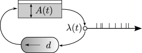
In the following we describe an extension of renewal theory for ensembles of point processes with time varying input. For stationary input rate, many previous publications have investigated the statistics of the PPD (Brenguier and Amodei, 1989; Yu and Fessler, 2000; Teich and McGill, 1976; Picinbono, 2009). In case of slowly varying input rates, expressions for mean and variance of detector counts have been derived (Vannucci and Teich, 1978), and recently a method was proposed to correct for clustered input events (Larsen and Kostinski, 2009). PPDs with non-stationary input rate have been employed as a model for the signal transduction in the auditory nerve (Turcott et al., 1994). A sudden switch of the input rate was found to induce strong transients of the ensemble output rate. These reflect a transiently perturbed equilibrium of the occupation numbers in our two-state model, and we quantitatively analyze this case for the PPD. Response transients to rapidly changing input, in fact, explain the relation between neural refractoriness and neural precision (Berry and Meister, 1998). Furthermore, periodic input profiles are known to be distorted by refractoriness (Johnson and Swami, 1983). Here we derive the mapping of periodic input to output in the steady state and uncover the impact of refractoriness on the transmission. Interacting populations of refractory neurons have been studied in (Wilson and Cowan, 1972). This approach, in contrast to ours, neglects the effects of refractoriness on short time scales due to temporal coarse-graining of the population dynamics.

From a more abstract perspective, the PPD is a very simple example of a point process that exhibits stochastic transients, which are not shared by the ordinary Poisson process. Besides its many applications, the PPD therefore is a prototype system to study non-equilibrium phenomena in point process dynamics. Generally, non-stationary point processes can be defined by two different models: by rescaling time (Brown et al., 2001; Reich et al., 1998; Nawrot et al., 2008) or by time-dependent parameters of the hazard. The drawback of the former method is that the transformation from operational to real time distorts the inter-event intervals, such that, for example, a constant refractory period is not maintained. An example how a time-dependent hazard function can be derived from an underlying neuron model with time-dependent input is given in (Muller et al., 2007). Our approach differs with regard to the choice of the hazard function, which enables rigorous analysis of the dynamics of the process.

To analytically investigate non-equilibrium phenomena in ensembles of renewal process, a typical approach is to use a partial differential equation (PDE) for the probability density of the ages of the components (time since the last event)(Gerstner and Kistler, 2002). In Section II we derive the two-state representation of the PPD from the dynamics of the age density. We present analytical solutions of the population dynamics for the response to a step change in the input rate in Section III, and to periodic input rate profiles in Section IV. Finally, in Section V, we generalize our results to random refractoriness. We compute the effective hazard function of the resulting inhomogeneous renewal process, connecting it to the framework of renewal theory. For the PPRD with gamma-distributed dead-times, as applied recently to model neural activity (Toyoizumi et al., 2009), we show how the dynamics in terms of a distributed delay differential equation can be reduced to a system of ordinary (non-delay) differential equations. Again we study the transient response of an ensemble of processes to a step-like change in the input rate and the transmission of periodic input. We observe that both distributed and fixed refractoriness lead to qualitatively similar dynamical properties. At last we identify the class of renewal processes that can be represented as a PPRD. As it turns out, this covers a wide range of renewal processes.

II Dynamics of an ensemble of PPDs

Point processes can be defined by a hazard function

$$h(t,\mathcal{H}_{t})\stackrel{{\scriptstyle\mathrm{def}}}{{=}}\lim_{\epsilon\to 0}\frac{1}{\epsilon}\mathbb{P}\left[\text{event in }[t,t+\epsilon]\,|\,\mathcal{H}_{t}\right],$$ (1)

which is the conditional rate of the process to generate an event at time $t$, given the history of event times $\mathcal{H}_{t}$ up until $t$. A process is a renewal process (Cox, 1967) if the hazard function depends only on the time $\tau$ since the last event (age) instead of the whole history $\mathcal{H}_{t}$. This can be generalized to the inhomogeneous renewal process which, additionally, allows for an explicit time dependence of the hazard function $h(t,\mathcal{H}_{t})=h(t,\tau)$.

Here we consider an ensemble of point processes defined by the hazard function

$$h(t,\tau)=\lambda(t)\theta(\tau-d),$$ (2)

where $\theta(t)=\{1\text{ for }t\geq 0,\;0\text{ else\}}$ denotes the Heaviside function, $d\geq 0$ is called dead-time, $\lambda(t)\geq 0$ is the time-dependent input rate and $\tau\geq 0$ is the age of the component process. This is an inhomogeneous renewal process, which is known as the Poisson process with dead-time (PPD). The state of an ensemble of such processes can be described by the time-dependent probability density of ages $a(t,\tau)$, for which a partial differential equation is known (Gerstner and Kistler, 2002)

$$\frac{\partial}{\partial t}a(t,\tau)=-\frac{\partial}{\partial\tau}a(t,\tau)-h(t,\tau)a(t,\tau).$$ (3)

Solutions must conserve probability, which manifests itself in the boundary condition $a(t,0)=\nu(t)$, with the event rate of the ensemble

$$\nu(t)\stackrel{{\scriptstyle\mathrm{def}}}{{=}}\int_{0}^{\infty}h(t,\tau)a(t,\tau)\,d\tau=\lambda(t)A(t).$$ (4)

In the second step we inserted (2) and introduced the active fraction of component processes with age $\tau\geq d$

$$A(t)\stackrel{{\scriptstyle\mathrm{def}}}{{=}}\int_{d}^{\infty}a(t,\tau)\,d\tau.$$ (5)

For $\tau<d$, Eq. (3) simplifies to $\partial_{t}a(t,\tau)=-\partial_{\tau}a(t,\tau)$, implying

$$a(t+u,u)=a(t,0)=\nu(t)\quad\forall u\in[0,d).$$ (6)

Since $a(t,\tau)$ is normalized we obtain with the boundary condition and (6),

$$1=\int_{0}^{\infty}a(t,\tau)\,d\tau=\int_{t-d}^{t}\nu(s)\,ds+A(t).$$ (7)

This equation is the starting point of the analysis of interacting populations of refractory neurons in (Wilson and Cowan, 1972). Differentiation of (7) by $t$ yields

$$\frac{d}{dt}A(t)=\lambda(t-d)A(t-d)-\lambda(t)A(t)\;,$$ (8)

which is a linear delay differential equation (DDE) with time-dependent coefficients. Its forward solution for input $\lambda(t)$ is uniquely defined given $A(t)$ on an interval of length $d$ (Bellman and Cooke, 1963). However, not all solutions of (8) can be interpreted physically, since by differentiation of (7) additive constants are lost. Only if the initial trajectory satisfies (7), Eq. (8) determines the time evolution of the ensemble. With (4), the time-dependent output rate $\nu(t)$ follows. Note that only in the case of the “pure” Poisson process with $d=0$ we obtain $\nu(t)=\lambda(t)$, because $A(t)=1$ by (7).

Eq. (8) represents a more accessible description of the process in terms of the occupation of the active and the refractory state (see Fig. 1 and Section I) compared to the dynamics of the probability density of ages (3). This description is feasible because of the particular nature of the hazard function of the PPD (2). In the following we will consider specific solutions of (8).

III Solutions for a step input

If $\lambda(t)=\lambda$ is constant, given the occupation $A(t)=u(t)$ on the first interval $t\in[-d,0]$ with $u:[-d,0]\to[0,1]$, solutions to (8) are known in integral form (Bellman and Cooke, 1963)

$$A(t)=u(0)g(t)+\int_{0}^{d}\lambda u(s-d)\,g(t-s)\,ds$$ (9)

for $t\geq 0$, where we introduced the fundamental solution $g(t)$. It obeys $g(t)=\{0\text{ for }t<0,\;1\text{ for }t=0\}$ and solves (8) for $t>0$. As we will show, here $g$ is in fact the shifted and scaled auto-correlation function $R$ of the process.

The inter-event interval density of the stationary PPD is $f(t)=\lambda\theta(t-d)e^{-\lambda(t-d)}$. For $t\geq d$, the integral equation

$$A(t)=(f\star A)(t),$$ (10)

is equivalent to the delay differential equation (8), which can be proven by differentiation with respect to $t$ ($\star$ denotes the convolution). The auto-correlation function (Cox, 1967)

$$R(t)=\sum_{k=0}^{\infty}f^{\star k}(t),$$ (11)

with $f^{\star k}(t)\stackrel{{\scriptstyle\mathrm{def}}}{{=}}(f^{\star(k-1)}\star f)(t)$ for $k\geq 1$ and $f^{\star 0}\stackrel{{\scriptstyle\mathrm{def}}}{{=}}\delta(t)$, solves (10) for $t\geq d$, and hence is a solution of (8) in that domain. We find for $k\geq 1$ that

$$f^{*k}(t)=\lambda^{k}(t-kd)^{k-1}e^{-\lambda(t-kd)}\theta(t-kd)/(k-1)!\,.$$ (12)

Given the initial trajectory $g(t)$ for $t\leq 0$, solving (8) by variation of constants for $t\in[0,d]$ yields $g(t)=\lambda^{-1}f(t+d)=\lambda^{-1}R(t+d)$. Then due to uniqueness of the solution it holds for all $t\geq 0$ that

$$g(t)=\lambda^{-1}R(t+d)\;.$$ (13)

We apply these results to compute the response of $A(t)$ if the input rate is switched from $\lambda_{0}$ to $\lambda$ at $t=0$, given the process was in equilibrium for $t\leq 0$. Eq. (7) determines this equilibrium to $A(t)\equiv a_{0}=(1+\lambda_{0}d)^{-1}$, $t\leq 0$. In this case, the step change in $\lambda(t)$ enters (9) as

$$A_{\mathrm{step}}(t)=u(0)g(t)+\int_{0}^{d}\underbrace{\lambda(s-d)}_{\lambda_{0}}u(s-d)\,g(t-s)\,ds,$$ (14)

for $t\geq 0$. We insert (13) to obtain

$$A_{\mathrm{step}}(t) = \frac{a_{0}}{\lambda}R(t+d)+\frac{\lambda_{0}a_{0}}{\lambda}\int_{0}^{d}R(t+d-s)\,ds$$ (15)

$$= \frac{a_{0}}{\lambda}R(t+d)+\frac{\lambda_{0}a_{0}}{\lambda}\left(1-\frac{1}{\lambda}R(t+d)\right)$$

$$= \frac{a_{0}\lambda_{0}}{\lambda}\left(1+(\lambda_{0}^{-1}-\lambda^{-1})\,R(t+d)\right),$$

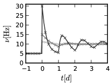
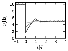
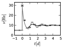
where we used (7), which holds for $g(t)=\lambda^{-1}R(t+d)$. Fig. 2 shows this analytical solution compared to direct numerical simulation of an ensemble of PPDs upon a step change of the input rate $\lambda(t)$ at $t=0$. The output rate displays a marked transient, which increases with the dead-time $d$ and exhibits oscillations of frequency $1/d$.

A	B

Figure 2: Transients upon step change of the input rate $\lambda(t)$ at $t=0$. Exact analytical result (15) (solid lines) and simulation of the ensemble rate of $10^{10}$ processes (crosses). Parameters: $d\,[\mathrm{s}]:$ $0.02,\,0.05,\,0.08$ (light gray, mid gray, dark gray) A: $\lambda_{0}=((5\mathrm{Hz})^{-1}-d)^{-1},\lambda=((10\mathrm{Hz})^{-1}-d)^{-1}$, B: $\lambda_{0}=((10\mathrm{Hz})^{-1}-d)^{-1},\lambda=((5\mathrm{Hz})^{-1}-d)^{-1}$.

IV Transmission of periodic input

We now investigate an ensemble of PPDs with an input rate $\lambda(t)\in\mathbb{R}$ that is periodic. If $T$ is its period, we obtain the Fourier series $\lambda(t)=\sum_{k=-\infty}^{\infty}\Lambda_{k}e^{ik\omega t}$, with $\omega=\frac{2\pi}{T}$ and $\Lambda_{k}\in\mathbb{C}$. Then the steady state solution for the active fraction $A(t)$ of the PPD is also periodic in $T$, so it can be expressed as $A(t)=\sum_{k=-\infty}^{\infty}\alpha_{k}e^{ik\omega t}$ with $\alpha_{k}\in\mathbb{C}$. Inserted into (7) we obtain

$$1=\sum_{k,l=-\infty}^{\infty}\Lambda_{l}\alpha_{k}q_{l+k}e^{i(l+k)\omega t}+\sum_{k=-\infty}^{\infty}\alpha_{k}e^{ik\omega t}$$ (16)

where for $k\neq 0$

$$\int_{t-d}^{t}e^{ik\omega t}\,dt=\frac{1-e^{-ik\omega d}}{ik\omega}e^{ik\omega t}\stackrel{{\scriptstyle\mathrm{def}}}{{=}}q_{k}e^{ik\omega t},$$

and $q_{0}\stackrel{{\scriptstyle\mathrm{def}}}{{=}}d$. Since the Fourier basis functions $\{e^{ik\omega t},k\in\mathbb{Z}\}$ are mutually orthogonal, we can separate (16) for different $k$. This yields the infinite dimensional linear system of equations

$$\delta_{k,0}=q_{k}\sum_{l=-\infty}^{\infty}\Lambda_{l}\alpha_{k-l}+\alpha_{k},\;k\in\mathbb{Z}.$$ (17)

The ensemble averaged output rate of the PPD defined in (4) then follows as $\nu(t)=\lambda(t)A(t)=\sum_{k=-\infty}^{\infty}\beta_{k}e^{ik\omega t}$ with the spectrum

$$\beta_{k}=\sum_{l=-\infty}^{\infty}\alpha_{k-l}\Lambda_{l}=q_{k}^{-1}\left(\delta_{k,0}-\alpha_{k}\right),$$ (18)

where we used (17). This given, we replace the $\alpha_{k}$ by $\beta_{k}$ in (17) to obtain

$$\beta_{k}=\Lambda_{k}-\sum_{l=-\infty}^{\infty}\Lambda_{k-l}q_{l}\beta_{l},\;k\in\mathbb{Z}.$$ (19)

This relation shows how different frequencies of the output rate are coupled by a convolution with the input spectrum. Note that inverting (19) yields the spectrum of the time-dependent input rate $\lambda(t)$ given the spectrum of the output rate signal $\nu(t)$.

Let us now consider the special case of a cosine-modulated input

$$\lambda(t)=\lambda_{0}+\epsilon\cos(\omega t),$$

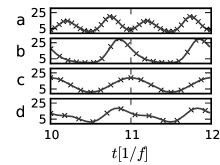
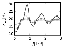
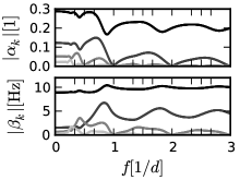
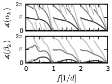
which we obtain with $\Lambda_{k}=\{0\text{ for }|k|>1\text{, }\frac{\epsilon}{2}\text{ for }k\in\{1,-1\},\,\lambda_{0}\text{ for }k=0\}$, $\lambda_{0}\geq\epsilon\geq 0$. Then for $k\in\mathbb{N}$, (17) becomes a so-called three-term recurrence relation (Gautschi, 1967) of the form $0=\alpha_{n+1}+x_{n}\alpha_{n}+y_{n}\alpha_{n-1}$ with $x_{n}=(q_{n}^{-1}+\lambda_{0})(2/\epsilon)$ and $y_{n}=1$. This relation has two linearly independent solutions. The unique minimal solution is convergent and can be obtained from the continued fraction $r_{n-1}=-y_{n}/(x_{n}+r_{n})$ in a robust manner (Gautschi, 1967) using the relation $r_{n}=\alpha_{n+1}/\alpha_{n},\,n\geq 0$: Setting $r_{N}=0$ for some $N\in\mathbb{N}$ one computes $(r_{n})_{0\leq n<N}$ backwards and increases $N$ until $r_{0}$ does not change within the required tolerance. Inserting $\alpha_{1}=r_{0}\alpha_{0}$ into (17) for $k=0$ we solve for $\alpha_{0}$ to obtain $\alpha_{0}=(1+d(\lambda_{0}+\epsilon\Re(r_{0})))^{-1}$ (here $\Re$ denotes the real part). The remaining $\alpha_{k}$ follow recursively from $\alpha_{k+1}=\alpha_{k}r_{k}$ and $\alpha_{-k}=\alpha_{k}^{\star}$, since $A(t)\in\mathbb{R}$. The spectrum of the output rate is then given by (18). Fig. 3A shows the output rate $\nu(t)$ for different input rate modulation frequencies $f=\omega/(2\pi)$. Fig. 3C,D display the amplitude and phase of the three lowest harmonics of the output rate $\nu(t)$ as a function of $f$. The time averaged emission rate ($\beta_{0}$) depends on the modulation frequency. It is maximized slightly below the characteristic frequencies $f=k/d$. This is due to the oscillation of $A(t)$, which is almost in phase at these frequencies and hence cooperates with the oscillatory hazard rate $\lambda(t)$ to enhance the emission (see Fig. 3D). Interestingly, the first ($\beta_{1}$) and second ($\beta_{2}$) harmonic of $\nu(t)$ display maxima at different $f$. At a particular modulation frequency $f\simeq 1/(2d)$ the amplitude of the second harmonic ($\beta_{2}$) is larger than the first harmonic ($\beta_{1}$), so that the ensemble activity is effectively modulated with twice the input frequency (see Fig. 3A (a) and Fig. 3C): the ensemble performs a frequency doubling. Fig. 3B shows the maximum over one period of the output rate trajectory. These maxima are dominated by the maxima of the amplitude of the first harmonic. In particular, low frequency input signals are transmitted to the output with strong distortion and reduced intensity, because the fraction of non-refractory processes, $A(t)$, is in anti-phase (Fig. 3D) to $\lambda(t)$ and hence suppresses the output rate’s modulation. This is in contrast to the common view that the PPD transmits slow signals more reliably than the Poisson process (Gerstner and Kistler, 2002). Note that only if the driving frequency $f=n/d$, $n\in N$ is an integer multiple of the inverse dead-time then $A(t)=(1+\lambda_{0}d)^{-1}$ is constant in time and the output rate is proportional to $\lambda(t)$ without any distortion.

A	B
C	D

Figure 3: Transmission of cosine-modulated input. A, B: Theoretical result (solid lines) and simulation of an ensemble of $10^{10}$ processes (crosses). A: Steady-state rate $\nu(t)$ for different modulation frequencies $f$, with $fd$: $0.42,\,0.85,\,1.0,\,1.4$ (a,b,c,d). B: $\nu_{\max}=\max(\nu(t))$ for different $f$. Here $d\,[\mathrm{s}]$: $0.02,\,0.05,\,0.08$ (light gray, mid gray, dark gray) C,D: Amplitude (C) and phase (D) of harmonics $k\in\{0,\ldots,3\}$ of $A(t)$ (19) (top) and $\nu(t)$ (18) (bottom) as a function of modulation frequency $f$. Grayscale denotes order of harmonics $k:$ $0,1,2,3$ (black, dark gray, mid gray, light gray), $d=80\mathrm{ms}$. Other parameters in A-D: $\lambda(t)=\lambda_{0}(1+0.9\cos(2\pi ft))$, $\lambda_{0}=(\nu_{0}^{-1}-d)^{-1}$, $\nu_{0}=10\mathrm{Hz}$.

V Random dead-time

For detector devices as well as for neurons, a fixed dead-time might be a somewhat restricted model. Here we consider the PPRD as described in the introduction. Upon generation of each event, the PPRD draws an independent and identically distributed random dead-time with the probability density function (PDF) $\rho$ for the duration of which it remains silent. The PPRD is still a renewal process, since it has no further dependencies on the event history beyond the time since the last event. As in the case of a fixed dead-time in Section II, the following analysis of the PPRD is based on the conservation of the total number of processes in an ensemble. Inactive components must have generated an event at some time in the past, which leads to the normalization condition

$$1=A(t)+\int_{-\infty}^{t}A(t^{\prime})\lambda(t^{\prime})\int_{t-t^{\prime}}^{\infty}\rho(x)dx\,dt^{\prime}\,.$$ (20)

This equation can be seen as the generalization of the normalization condition (7), from which the DDE (8) follows by differentiation, to the case of random dead-time. Analogously the distributed DDE

$$\frac{d}{dt}A(t)=-\lambda(t)A(t)+\int_{0}^{\infty}\rho(x)\lambda(t-x)A(t-x)\,dx$$ (21)

follows from (20) by differentiation with respect to $t$. Eq. (21) describes the time-evolution of the occupation of the active state for an ensemble of general PPRDs. Obviously, the dynamics of the PPD (8) is recovered from (21) in case of the localized density $\rho(x)=\delta(x-d)$. In the rest of this section, we will derive the hazard function $h(t,\tau)$ of the PPRD, consider the case of gamma-distributed dead time and the associated step response, generalize the transmission of periodic input to random dead-time, and finally identify the class of renewal processes that can be represented by the PPRD.

For a given density $\rho(x)$ of the dead-time it is not obvious what the hazard function of the PPRD is. In order to relate the PPRD to renewal theory we compute its time-dependent hazard function (1) here. Let

$$Q(t,\tau)\stackrel{{\scriptstyle\mathrm{def}}}{{=}}\mathbb{E}\left[\theta(\tau-x)|\,\text{last event at }t-\tau\right]$$

denote the probability of the process to be active at time $t$, given the last event occured at $t-\tau$, where $x$ is the random dead-time and $\mathbb{E}$ denotes the expectation value with respect to $x$. The hazard function is then $h(t,\tau)=\lambda(t)Q(t,\tau)$. With

$$Q(t,\tau)=\mathbb{P}\left[x<\tau\,|\,\text{last event at }t-\tau\right]\\ =1-\mathbb{P}\left[x\geq\tau\,|\,\text{ev. at }t-\tau\,\cap\,\text{no ev. in }(t-\tau,t)\right]\\ =1-\mathbb{P}\left[x\geq\tau\right]/\mathbb{P}\left[\text{no ev. in }(t-\tau,t)\,|\,\text{ev. at }t-\tau\right]$$

we obtain

$$h(t,\tau) = \lambda(t)\left(1-\mathcal{F}(\tau)/\mathbb{E}\left[F(t,\tau|x)\right]\right),$$ (22)

where

$$\mathcal{F}(\tau)=\int_{\tau}^{\infty}\rho(x)dx$$

is the survivor function of the dead-time distribution and

$$F(t,\tau|x)=\exp(-\theta(\tau-x)\int_{t-\tau+x}^{t}\lambda(t^{\prime})dt^{\prime})$$

is the survivor function of a PPD with dead-time $x$. In case of constant $\lambda(t)=\lambda$ we further have

$$\mathbb{E}\left[F(t,\tau|x)\right]=e^{-\lambda\tau}\int_{0}^{\tau}e^{\lambda x}\rho(x)dx+\mathcal{F}(\tau).$$

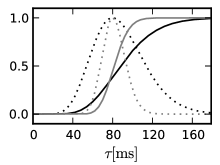
The hazard function (22) is shown for constant $\lambda(t)$ in Fig. 4A for the special case described below. Eq. (22) was applied to generate realizations of the PPRD for Fig. 4B.

For gamma-distributed dead-time (8) can be transformed into a system of ordinary differential equations. We exemplify the application of (21) for gamma distributed dead-times with parameters $n\in\mathbb{N}$ and $\beta\in\mathbb{R}^{+}$,

$$\rho(x) = \kappa_{n}(x),$$ (23)

$$\kappa_{n}(x) = \beta^{n+1}x^{n}e^{-\beta x}/n!\,,$$ (24)

with $\mathbb{E}[x]=(n+1)/\beta$. The time course of the rate can be obtained from (21). Introducing

$$b_{k}(t)\stackrel{{\scriptstyle\mathrm{def}}}{{=}}\int_{-\infty}^{t}\kappa_{k}(t-x)\nu(x)\,dx$$

for $0\leq k\leq n$ and $b_{n+1}(t)\stackrel{{\scriptstyle\mathrm{def}}}{{=}}A(t)$ and exploiting the relation

$$\frac{d}{dx}\kappa_{k}(x) = \theta(k-1)\beta\kappa_{k-1}(x)-\beta\kappa_{k}(x)$$

for $0\leq k\leq n$ enables to replace the integral in (21) by a closed system of ordinary differential equations

$$\frac{d}{dt}b_{k}(t) = \begin{cases}-b_{n+1}(t)\lambda(t)+b_{n}(t)&k=n+1\\ \beta b_{k-1}(t)-\beta b_{k}(t)&1\leq k\leq n\\ \beta b_{n+1}(t)\lambda(t)-\beta b_{0}(t)&k=0.\end{cases}$$ (25)

For constant $\lambda(t)=\lambda$ this can be written as $\frac{d}{dt}\vec{b}(t)=\mathbf{M}_{\lambda}\,\vec{b}(t)$, $\vec{b}(t)\in\mathbb{R}^{n+2}$. Hence given the initial state $\vec{b}(0)$ the solution unfolds to

$$\vec{b}(t) = \exp(\mathbf{M}_{\lambda}t)\cdot\vec{b}(0)\,.$$ (26)

With $\nu(t)=\nu=(\lambda^{-1}+\mathbb{E}[x])^{-1}$ the equilibrium state follows: Setting the temporal derivatives to $0$ in (25) yields $b_{k}=\nu$ for $0\leq k\leq n$, and $b_{n+1}=A=1-\nu\mathbb{E}[x]$. The rate response to a switch from $\lambda_{0}$ to $\lambda$ at $t=0$ is thus given by (26) where $\vec{b}(0)$ is the equilibrium state for $\lambda_{0}$. A numerical simulation of the process with gamma distributed refractoriness (23) with hazard function (22) and the corresponding analytical solution (26) upon a step change of $\lambda(t)$ are shown in Fig. 4. The simulation of the process was done via rejection (Ripley, 1987) and averaged over independent runs. The spread of dead-times (Fig. 4A) does not qualitatively change the shape of the response transient (Fig. 4B).

Analogous to Section IV, we consider the case of periodic input. We insert the Fourier series of $\lambda(t)$ and $A(t)$ into (20) and obtain the same relation of their spectra (16) as for a single dead-time with the altered coefficients

$$q_{k}=\int_{0}^{\infty}e^{-ik\omega y}\int_{y}^{\infty}\rho(x)dx\,dy.$$ (27)

As is easily seen, by inserting the localized dead-time PDF $\rho(x)=\delta(x-d)$ the original $q_{k}$ are recovered. Hence all results of Section IV also hold for the PPRD, but with the coefficients (27). In particular we would like to emphasize the validity of the general input-output mapping (19) for arbitrarily distributed dead-time.

Let us now investigate which class of renewal processes can be represented by the PPRD. We start with an arbitrary renewal process with inter-event interval $I\in\mathbb{R}_{+}$, defined by its PDF $\iota(x)$. Let $E\geq 0$ be an independent, exponentially distributed interval with PDF $\epsilon(x)=\lambda e^{-\lambda x}$, and let $R$ be the random dead-time with PDF $\rho(x)$. For $I$ to be a realization of a PPRD it must hold for some $\rho$ and $\lambda\geq 0$ that

$$I=R+E\Rightarrow\iota=\rho\star\epsilon\Rightarrow\hat{\iota}=\hat{\rho}\hat{\epsilon}\\ \Rightarrow\hat{\rho}=\lambda^{-1}(s+\lambda)\hat{\iota}\Rightarrow\rho=\lambda^{-1}\mathcal{L}^{-1}\left[s\hat{\iota}\right]+\iota\\ \Rightarrow\rho(x)=\frac{1}{\lambda}\left(\frac{d}{dx}\iota(x)+\iota(0)\right)+\iota(x),$$ (28)

where $\hat{\,}$ decorates a function which was transformed by the Laplace transform $\mathcal{L}$, and $s$ denotes the Laplace variable. The renewal process defined by $\iota$ can be represented by a PPRD if $\rho$ is a PDF. Let us call the hazard function of the renewal process $h(x)$, and the survivor function $F(x)=\exp(-\int_{0}^{x}h(x^{\prime})dx^{\prime})$, which obey $\iota(x)=h(x)F(x)$ (Cox, 1967). Assume that $\iota(x)$ is differentiable. Since expression (28) is always normalized, in order for it to define a suitable PDF we only have to require $\rho(x)\geq 0$ for all $x$, possibly in the sense of distributions. This translates into

$$\lambda^{-1}\left(h^{\prime}(x)-h^{2}(x)\right)+h(x)\geq 0.$$ (29)

In case $h(x)>0$, this can be written as

$$h(x)-\frac{h^{\prime}(x)}{h(x)}\leq\lambda.$$ (30)

If, in addition, the hazard and its derivative are bounded in the sense that $h(x)<\infty$ and $h^{\prime}(x)>-\infty$, there exists a $\lambda>0$ such that (30) is fulfilled. These conditions are indeed met by a large class of renewal processes.

For example, the gamma-process which has random inter-event intervals with PDF $\iota(x)=\kappa_{r}(x)$ (23) with parameters $r,\beta\in\mathbb{R}$, $r\geq 1$, $\beta\geq 0$ is by (28) equivalent to the PPRD with $\rho(x)=\kappa_{r-1}(x)$ and $\lambda=\beta$, but other choices of $\lambda$ are also possible. This illustrates the well known fact that the inter-event intervals of gamma processes with integer shape parameter $n$ can be considered as the concatenation of $n$ exponentially distributed intervals. In neuroscience the gamma-process is frequently used to model stationary time series of action potential emissions of nerve cells. To describe adaptation phenomena, a time-dependence of the parameters of the hazard function was introduced in (Muller et al., 2007). Identification of the gamma-process with a PPRD entails the alternative to generalize the gamma process to time-dependent rates by varying the input rate of the PPRD. Similarly, the log-normal process can be represented as a PPRD. We define its inter-event interval as $x=\xi\Delta$, where $\xi$ is a unit-less random number and $\Delta$ gives the time-scale. Let $\xi$ be distributed according to the log-normal PDF

$$\eta(\xi) = \frac{1}{\sqrt{2\pi}\xi\sigma}\exp\left(-\frac{(\log\xi-\mu)^{2}}{2\sigma^{2}}\right)$$

for $\xi>0$, $\eta(0)=0$, with unit-less parameters $\mu,\,\sigma$. Then $x$ is distributed according to $\iota(x)=\Delta^{-1}\eta(\nicefrac{{x}}{{\Delta}})$. According to (28) the process can be represented by any of the PPRDs with

$$\rho(x) = \iota(x)\left(1-\frac{1}{x\lambda}\left(1+\frac{\log\frac{x}{\Delta}-\mu}{\sigma^{2}}\right)\right)$$

$$\lambda \geq \Delta^{-1}\sigma^{-2}\exp\left(-1-\mu+\sigma^{2}\right),$$

where the lower bound on $\lambda$ is due to the requirement $\rho(x)\geq 0$. For these and other renewal processes for which a PPRD representation exists, non-equilibrium dynamics can be studied on the basis of (21).

A	B

Figure 4: PPD with random dead-time with mean $80\mathrm{ms}$, shape parameter $n$: $10,\,50$ (black, gray). A: density of dead-times $\rho(\tau)/\max(\rho(\tau))$ (23) (dotted lines) and hazard function $h(\tau)/\lambda_{0}$ (22) for $\lambda(t)=\lambda_{0}$ (solid lines). B: Transients upon step change of the input rate $\lambda(t)$ at $t=0$. Theoretical result from (26) (solid lines) and simulation of an ensemble of $10^{6}$ processes with hazard function (22) (crosses) averaged over 225 trials. The error bars denote the standard deviation over trials. $\lambda_{0}=((5\mathrm{Hz})^{-1}-d)^{-1},\,\lambda=((10\mathrm{Hz})^{-1}-d)^{-1}$.

VI Discussion

In this paper, we consider the effect of refractoriness on the output of an encoding point process in case of arbitrary time-dependent input signals. Such point processes, for example, are used to model the generation of action potentials by nerve cells, the release and reuptake of vesicles into the synaptic cleft, or the detection of particles by technical devices. We describe ensembles of these stochastic processes by the occupation numbers of two states: active and refractory. The active components behave as inhomogeneous Poisson processes, but after an event is produced the component is silent for the duration of the dead-time, it is caught in a delay line. We derive a distributed delay differential equation that describes the dynamics in the general case of a randomly distributed dead-time.

Due to the simpler dynamics in case of a fixed dead-time, we first elaborate properties of the PPD. For stationary input rate, we solve the dynamics of the ensemble in a way that sheds light on the connection between the fundamental solution of the DDE and the auto-correlation function of the point process. This relation is employed to express the time-dependent ensemble rate (output) for a step-change of the hazard rate (input). The resulting output rate displays stochastic transients and oscillations with a periodicity given by the dead-time. Such transients might enable nerve cells to respond reliably to rapid changes in the input currents (Mainen and Sejnowski, 1995; Berry and Meister, 1998). For periodically modulated input rate, we demonstrate how the spectrum of the steady-state periodic output rate results from the linear coupling between harmonics. In the particular case of cosine-modulated input signals only adjacent harmonics are coupled. This nearest-neighbor interaction is rigorously solved using the theory of three-term-recurrence relations and continued fractions (Gautschi, 1967).

Our analytic result explains frequency doubling, the emergence of higher harmonics and the dependence of the time averaged population activity on the modulation frequency. In particular, slow frequency components of the input are attenuated and distorted in the population rate, which is in contrast to the claim that the PPD transmits slow frequency signals more reliably than the Poisson process (Gerstner and Kistler, 2002).

In case of periodic input modulation, the output spectrum contains all harmonics of the fundamental frequency of the input. This might be related to a psychophysical phenomenon called “missing fundamental illusion” (Schouten, 1940; Licklider, 1951): Being presented an auditory stimulus which consists of several harmonics of a fundamental frequency, but in which the fundamental frequency itself is missing, subjects nonetheless perceive the fundamental frequency as if it was contained in the stimulus spectrum. By considering neurons in the auditory system as PPDs whose hazard rate is modulated by the auditory stimulus, our theory explains how the lowest harmonic is recovered in the population activity of the neurons. Conversely, our results can be applied to infer input rate profiles from the count rate of detectors with dead-time, in particular in the case of periodic input, for which (19) applies.

For the more general case of a random, arbitrarily distributed dead-time, we show how the DDE generalizes to a distributed DDE. By suitable choice of the distribution of the dead-time, non-equilibrium dynamics of a large class of renewal processes can be described. For integer gamma-distributed dead-time we demonstrate how the distributed DDE transforms into a coupled system of finitely many ordinary differential equations, which could also be implemented as a multi-state Markov system (Toyoizumi et al., 2009). Regarding the output rate transient upon a step change of the input and the transmission of periodic inputs, we find that the qualitative behavior of the system is very similar to the PPD. In conclusion, we present a canonical model for non-stationary renewal processes, as well as the analytical methods to describe ensembles thereof.