Bayesian computational methods
Christian P. Robert Université Paris-Dauphine, CEREMADE, and CREST, INSEE, Paris

0.1 Introduction

If, in the mid 1980’s, one had asked the average statistician about the difficulties of using Bayesian Statistics, the most likely answer would have been “Well, there is this problem of selecting a prior distribution and then, even if one agrees on the prior, the whole Bayesian inference is simply impossible to implement in practice!” The same question asked in the 21th Century does not produce the same reply, but rather a much less aggressive complaint about the lack of generic software (besides winBUGS), along with the renewed worry of subjectively selecting a prior! The last 20 years have indeed witnessed a tremendous change in the way Bayesian Statistics are perceived, both by mathematical statisticians and by applied statisticians and the impetus behind this change has been a prodigious leap-forward in the computational abilities. The availability of very powerful approximation methods has correlatively freed Bayesian modelling, in terms of both model scope and prior modelling. This opening has induced many more scientists from outside the statistics community to opt for a Bayesian perspective as they can now handle those tools on their own. As discussed below, a most successful illustration of this gained freedom can be seen in Bayesian model choice, which was only emerging at the beginning of the MCMC era, for lack of appropriate computational tools.

In this chapter, we will first present the most standard computational challenges met in Bayesian Statistics (Section 0.2), and then relate these problems with computational solutions. Of course, this chapter is only a terse introduction to the problems and solutions related to Bayesian computations. For more complete references, see Robert and Casella (2004), Marin and Robert (2007a), Robert and Casella (2004) and Liu (2001), among others. We also restrain from providing an introduction to Bayesian Statistics per se and for comprehensive coverage, address the reader to Marin and Robert (2007a) and Robert (2007), (again) among others.

0.2 Bayesian computational challenges

Bayesian Statistics being a complete inferential methodology, its scope encompasses the whole range of standard statistician inference (and design), from point estimation to testing, to model selection, and to non-parametrics. In principle, once a prior distribution has been chosen on the proper space, the whole inferential machinery is set and the computation of estimators is usually automatically derived from this setup. Obviously, the practical or numerical derivation of these procedures may be exceedingly difficult or even impossible, as we will see in a few selected examples. Before, we proceed with an incomplete typology of the categories and difficulties met by Bayesian inference. First, let us point out that computational difficulties may originate from one or several of the following items:

1. use of a complex parameter space, as for instance in constrained parameter sets like those resulting from imposing stationarity constraints in dynamic models;

2. use of a complex sampling model with an intractable likelihood, as for instance in missing data and graphical models;

3. use of a huge dataset;

4. use of a complex prior distribution (which may be the posterior distribution associated with an earlier sample);

5. use of a complex inferential procedure.

0.2.1 Bayesian point estimation

In a formalised representation of Bayesian inference, the statistician is given (or selects) a triplet

• a sampling distribution, $f(x|\theta)$, usually associated with an observation (or a sample) $x$;

• a prior distribution $\pi(\theta)$, defined on the parameter space $\Theta$;

• a loss function $\mathrm{L}(\theta,d)$ that compares the decisions (or estimations) $d$ for the true value $\theta$ of the parameter.

Using $(f,\pi,\mathrm{L})$ and an observation $x$, the Bayesian inference is always given as the solution to the minimisation programme

$$\min_{d}\,\int_{\Theta}L(\theta,d)\,f(x|\theta)\,\pi(\theta)\,\text{d}\theta\,,$$

equivalent to the minimisation programme

$$\min_{d}\,\int_{\Theta}L(\theta,d)\,\pi(\theta|x)\,\text{d}\theta\,.$$

The corresponding procedure is thus associated, for every $x$, to the solution of the above programme (see, e.g. Robert, 2007, Chap. 2).

There are therefore two levels of computational difficulties with this resolution: first the above integral must be computed. Second, it must be minimised in $d$. For the most standard losses, like the traditional squared error loss,

$$\mathrm{L}(\theta,d)=\left|\theta-d\right|^{2},$$

the solution to the minimisation problem is universally known. For instance, for the squared error loss, it is the posterior mean,

$$\int_{\Theta}\theta\,\pi(\theta|x)\,\text{d}\theta=\int_{\Theta}\theta\,f(x|\theta)\,\pi(\theta)\,\text{d}\theta\bigg{/}\int_{\Theta}f(x|\theta)\,\pi(\theta)\,\text{d}\theta\,,$$

which still requires the computation of both integrals and thus whose complexity depends on the complexity of $\Theta$, $f(x|\theta)$, and $\pi(\theta)$.

Example 1

For a normal distribution $\mathcal{N}(\theta,1)$, the use of a so-called conjugate prior (see, e.g., Robert, 2007, Chap. 3)

$$\theta\sim\mathcal{N}(\mu,\epsilon)\,,$$

leads to a closed form expression for the mean, since

$$\int_{\Theta} \theta\,f(x|\theta)\,\pi(\theta)\,\text{d}\theta\bigg{/}\int_{\Theta}f(x|\theta)\,\pi(\theta)\,\text{d}\theta=$$

$$\int_{\mathbb{R}} \theta\exp\frac{1}{2}\left\{-\theta^{2}(1+\epsilon^{-2})+2\theta(x+\epsilon^{-2}\mu)\right\}\text{d}\theta$$

$$\qquad\bigg{/}\int_{\mathbb{R}}\exp\frac{1}{2}\left\{-\theta^{2}(1+\epsilon^{-2})+2\theta(x+\epsilon^{-2}\mu)\right\}\text{d}\theta=\frac{x+\epsilon^{-2}\mu}{1+\epsilon^{-2}}\,.$$

On the other hand, if we use instead a more involved prior distribution like a poly-$t$ distribution (Bauwens and Richard, 1985),

$$\pi(\theta)=\prod_{i=1}^{k}\left[\alpha_{i}+(\theta-\beta_{i})^{2}\right]^{-\nu_{i}}\qquad\alpha,\nu>0$$

the above integrals cannot be computed in closed form anymore. This is not a toy example in that the problem may occur after a sequence of $k$ Student’s $t$ observations, or with a sequence of normal observations whose variance is unknown.

The above example is one-dimensional, but, obviously, bigger challenges await the Bayesian statistician when she wants to tackle high-dimensional problems.

Example 2

In a generalised linear model, a conditional distribution of $y\in\mathbb{R}$ given $x\in\mathbb{R}^{p}$ is defined via a density from an exponential family

$$y|x\sim\exp\left\{y\cdot\theta(x)-\psi(\theta(x))\right\}$$

whose natural parameter $\theta(x)$ depends on the conditioning variable $x$,

$$\theta(x)=g(\beta^{\mathrm{T}}x)\,,\qquad\beta\in\mathbb{R}^{p}$$

that is, linearly modulo the transform $g$. Obviously, in practical applications like Econometrics, $p$ can be quite large. Inference on $\beta$ (which is the true parameter of the model) proceeds through the posterior distribution (where $\mathbf{x}=(x_{1},\ldots,x_{T})$ and $\mathbf{y}=(y_{1},\ldots,y_{T})$)

$$\pi(\beta|\mathbf{x},\mathbf{y}) \propto\prod_{t=1}^{T}\exp\left\{y_{t}\cdot\theta(x_{t})-\psi(\theta(x_{t}))\right\}\,\pi(\beta)$$

$$=\exp\left\{\sum_{t=1}^{T}y_{t}\cdot\theta(x_{t})-\sum_{t=1}^{T}\psi(\theta(x_{t}))\right\}\,\pi(\beta)\,,$$

which rarely is available in closed form. In addition, in some cases $\psi$ may be costly simply to compute and in others $T$ may be large or even very large. Take for instance the case of the dataset processed by Abowd et al. (1999), which covers twenty years of employment histories for over a million workers, with $x$ including indicator variables for over one hundred thousand companies.

Complexity starts sharply increasing if we introduce in addition random effects to the model, that is writing $\theta(x)$ as $g(\beta^{\mathrm{T}}x+\epsilon(x))$, where $\epsilon(x)$ is a random perturbation indexed by $x$. For instance, in the above employment dataset, it may correspond to a worker effect or to a company effect. The difficulty is that those random variables can very rarely be integrated out into a closed-form marginal distribution. They must therefore be included within the model parameter, which then increases its dimension severalfold.

A related, although conceptually different, inferential issue concentrates upon prediction, that is, the approximation of a distribution related with the parameter of interest, say $g(y|\theta)$, based on the observation of $x\sim f(x|\theta)$. The predictive distribution is then defined as

$$\pi(y|x)=\int_{\Theta}g(y|\theta)\pi(\theta|x)\text{d}\theta\,.$$

A first difference with the standard point estimation perspective is obviously that the parameter $\theta$ vanishes through the integration. A second and more profound difference is that this parameter is not necessarily well-defined anymore. As will become clearer in a following Section, this is a paramount feature in setups where the model is not well-defined and where the statistician hesitates between several (or even an infinity of) models. It is also a case where the standard notion of identifiability is irrelevant, which paradoxically is a ”plus” from the computational point of view, as seen below in, e.g., Example 13.

Example 3

Recall that an $AR(p)$ model is given as the auto-regressive representation of a time series,

$$x_{t}=\sum_{i=1}^{p}\theta_{i}x_{t-i}+\sigma\varepsilon_{t}\;.$$

It is often the case that the order $p$ of the $AR$ model is not fixed a priori, but has to be determined from the data itself. Several models are then competing for the “best” fit of the data, but if the prediction of the next value $x_{t+1}$ is the most important part of the inference, the order $p$ chosen for the best fit is not really relevant. Therefore, all models can be considered in parallel and aggregated through the predictive distribution

$$\pi(x_{t+1}|x_{t},\ldots,x_{1})\propto\int f(x_{t+1}|x_{t},\ldots,x_{t-p+1})\pi(\theta,p|x_{t},\ldots,x_{1})\text{d}p\,\text{d}\theta\,,$$

which thus amounts to integrating over the parameters of all models, simultaneously:

$$\sum_{p=0}^{\infty}\int f(x_{t+1}|x_{t},\ldots,x_{t-p+1})\pi(\theta|p,x_{t},\ldots,x_{1})\,\text{d}\theta\,\pi(p|x_{t},\ldots,x_{1})\,.$$

Note the multiple layers of complexity in this case:

1. if the prior distribution on $p$ has an infinite support, the integral simultaneously considers an infinity of models, with parameters of unbounded dimensions;

2. the parameter $\theta$ varies from model $AR(p)$ to model $AR(p+1)$, so must be evaluated differently from one model to another. In particular, if the stationarity constraint usually imposed in these models is taken into account, the constraint on $(\theta_{1},\ldots,\theta_{p})$ varies between model $AR(p)$ and model $AR(p+1)$;

3. prediction is usually used sequentially: every tick/second/hour/day, the next value is predicted based on the past values $x_{t},\ldots,x_{1})$. Therefore when $t$ moves to $t+1$, the entire posterior distribution $\pi(\theta,p|x_{t},\ldots,x_{1})$ must be re-evaluated again, possibly with a very tight time constraint as for instance in financial or radar tracking applications.

We will discuss this important problem in deeper details after the testing section, as part of the model selection problematic.

0.2.2 Testing hypotheses

A domain where both the philosophy and the implementation of Bayesian inference are at complete odds with the classical approach is the area of testing of hypotheses. At a primary level, this is obvious when opposing the Bayesian evaluation of an hypothesis $H_{0}:\theta\in\Theta_{0}$

$$\hbox{Pr}^{\pi}(\theta\in\Theta_{0}|x)$$

with a Neyman–Pearson $p$-value

$$\sup_{\theta\in\Theta_{0}}\,\mbox{Pr}_{\theta}(T(X)\geq T(x))$$

where $T$ is an appropriate statistic, with observed value $T(x)$. The first quantity involves an integral over the parameter space, while the second provides an evaluation over the observational space. At a secondary level, the two answers may also strongly disagree even when the number of observations goes to infinity, although there exist cases and priors for which they agree to the order $\mathrm{O}(n^{-1})$ or even $\mathrm{O}(n^{-3/2})$. (See Robert, 2007, Section 3.5.5 and Chapter 5, for more details.)

From a computational point of view, most Bayesian evaluations of the relevance of an hypothesis—also called the evidence—given a sample $x$ involve marginal distributions

$$\int_{\Theta_{i}}f(x|\theta_{i})\pi_{i}(\theta_{i})\,\text{d}\theta_{i}$$ (1)

where $\Theta_{i}$ and $\pi_{i}$ denote the parameter space and the corresponding prior, respectively, under hypothesis $H_{i}$ $(i=0,1)$. For instance, the Bayes factor is defined as the ratio of the posterior probabilities of the null and the alternative hypotheses over the ratio of the prior probabilities of the null and the alternative hypotheses, i.e.,

$$B^{\pi}_{01}(x)=\dfrac{\text{Pr}(\theta\in\Theta_{0}\mid x)}{\text{Pr}(\theta\in\Theta_{1}\mid x)}\bigg{/}\dfrac{\pi(\theta\in\Theta_{0})}{\pi(\theta\in\Theta_{1})}.$$

This quantity is instrumental in the computation of the posterior probability

$$\text{Pr}(\theta\in\Theta_{0}\mid x)=\frac{1}{1+B^{\pi}_{10}(x)}$$

under equal prior probabilities for both $\Theta_{0}$ and $\Theta_{1}$. It is also the central tool in practical (as opposed to decisional) Bayesian testing (Jeffreys, 1961) and can be seen as the Bayesian equivalent of the likelihood ratio.

The first ratio in $B^{\pi}_{01}(x)$ is then the ratio of integrals of the form (1) and it is rather common to face difficulties in the computation of both integrals.

Example 4 (Continuation of Example 2)

In the case of the generalised linear model, a standard testing situation is to decide whether or not a factor, $x_{1}$ say, is influential on the dependent variable $y$. This is often translated as testing whether or not the corresponding component of $\beta$, $\beta_{1}$, is equal to $0$, i.e. $\Theta_{0}=\{\beta;\beta_{1}=0\}$. If we denote by $\beta_{-1}$ the other components of $\beta$, the Bayes factor for this hypothesis will be

$$\int_{\mathbb{R}^{p}}\exp \left\{\sum_{t=1}^{T}y_{t}\cdot g(\beta^{\mathrm{T}}x_{t})-\sum_{t=1}^{T}\psi(g(\beta^{\mathrm{T}}x_{t}))\right\}\,\pi(\beta)\,\text{d}\beta\bigg{/}$$

$$\int_{\mathbb{R}^{p-1}} \exp\left\{\sum_{t=1}^{T}y_{t}\cdot g(\beta^{\mathrm{T}}_{-1}(x_{t})_{-1})-\sum_{t=1}^{T}\psi(\beta^{\mathrm{T}}_{-1}(x_{t})_{-1})\right\}\,\pi_{-1}(\beta_{-1})\,\text{d}\beta_{-1}\,,$$

when $\pi_{-1}$ is the prior constructed for the null hypothesis and when the prior weights of $H_{0}$ and of the alternative are both equal to $1/2$. Obviously, besides the normal conjugate case, both integrals cannot be computed in a closed form.

In a related manner, confidence regions are also mostly intractable, being defined through the solution to an implicit equation. Indeed, the Bayesian confidence region for a parameter $\theta$ is defined as the highest posterior region,

$$\left\{\theta;\pi(\theta|x)\geq k(x)\right\}\,$$ (2)

where $k(x)$ is determined by the coverage constraint

$$\hbox{Pr}^{\pi}(\pi(\theta|x)\geq k(x)|x)=\alpha\,,$$

$\alpha$ being the confidence level. While the normalising constant is not necessary to construct a confidence region, the resolution of the implicit equation (2) is rarely straightforward! However, simulation-based equivalents generally produce acceptable approximations in a straightforward manner when both the prior and the likelihood can be numerically computed.

Example 5

Consider a binomial observation $x\sim\mathcal{B}(n,\theta)$ with a conjugate prior distribution, $\theta\sim\mathcal{B}e(\gamma_{1},\gamma_{2})$. In this case, the posterior distribution is available in closed form,

$$\theta|x\sim\mathcal{B}e(\gamma_{1}+x,\gamma_{2}+n-x)\,.$$

However, the determination of the $\theta$’s such that

$$\theta^{\gamma_{1}+x-1}(1-\theta)^{\gamma_{2}+n-x-1}\geq k(x)$$

with

$$\hbox{Pr}^{\pi}\left(\theta^{\gamma_{1}+x-1}(1-\theta)^{\gamma_{2}+n-x-1}\geq k(x)|x\right)=\alpha$$

is not possible analytically. It actually implies two levels of numerical difficulties:

1. find the solution(s) to $\theta^{\gamma_{1}+x-1}(1-\theta)^{\gamma_{2}+n-x-1}=k$,

2. find the $k$ corresponding to the right coverage,

and each value of $k$ examined in step 2. requires a new resolution of step 1. However, $k$ can also be interpreted as the $(1-\alpha)$ quantile of the random variable $\theta^{\gamma_{1}+x-1}(1-\theta)^{\gamma_{2}+n-x-1}$, hence derived from a large sample of $\theta$’s in a Monte Carlo perspective.

The setting is usually much more complex when $\theta$ is a multidimensional parameter, because the interest is usually in getting marginal confidence sets. Example 2 is an illustration of this setting: deriving a confidence region on one component, $\beta_{1}$ say, first involves computing the marginal posterior distribution of this component. As in Example 4, the integral

$$\int_{\mathbb{R}^{p-1}}\exp\left\{\sum_{t=1}^{T}y_{t}\cdot g(\beta^{\mathrm{T}}x_{t})-\sum_{t=1}^{T}\psi(\beta^{\mathrm{T}}x_{t})\right\}\,\pi_{-1}(\beta_{-1})\,\text{d}\beta_{-1}\,,$$

which is proportional to $\pi(\beta_{1}|x)$, is most often intractable. Fortunately, the simulation approximations mentioned above are also available to bypass this integral computation.

0.2.3 Model choice

Although they are essentially identical from a conceptual viewpoint, we do distinguish here between model choice and testing, partly because the former leads to further computational difficulties, and partly because it encompasses a larger scope of inferential goals than mere testing. Note first that model choice has been the subject of considerable effort in the past decades, and has seen many advances, including the coverage of problems of higher complexity and the introduction of new concepts. We stress that such advances mostly owe to the introduction of new computational methods.

As discussed in further details in Robert (2007, Chapter 7), the inferential action related with model choice does take place on a wider scale than simple testing: it covers and compares models, rather than parameters, which makes the sampling distribution $f(x)$ “more unknown” than simply depending on an undetermined parameter. In some respect, it is thus closer to estimation than to regular testing. In any case, it requires a more precise evaluation of the consequences of choosing the “wrong” model or, equivalently of deciding which model is the most appropriate for the data at hand. It is thus both broader and less definitive than deciding whether $H_{0}:\,\theta_{1}=0$ is true. At last, the larger inferential scope mentioned in the first point means that we are leaving for a while the well-charted domain of solid parametric models.

From a computational point of view, model choice involves more complex structures that, almost systematically, require advanced tools, like simulation methods which can handle collections of parameter spaces (also called spaces of varying dimensions), specially designed for model comparison.

Example 6

A mixture of distributions is the representation of a distribution (density) as the weighted sum of standard distributions (densities). For instance, a mixture of Poisson distributions, denoted as

$$\sum_{i=1}^{k}p_{i}{\mathcal{P}}(\lambda_{i})\,$$

has the following density:

$$\hbox{Pr}(X=k)=\sum_{i=1}^{k}p_{i}\,\frac{\lambda_{i}^{k}}{k!}\,e^{-\lambda_{i}}\,.$$

This representation of distributions is multi-faceted and can be used in populations with known heterogeneities (in which case a component of the mixture corresponds to an homogeneous part of the population) as well as a non-parametric modelling of unknown populations. This means that, in some cases, $k$ is known and, in others, it is both unknown and part of the inferential problem.

First, consider the setting where several (parametric) models are in competition,

$${\mathfrak{M}}_{i}:x\sim f_{i}(x|\theta_{i}),\qquad\theta_{i}\in\Theta_{i},\quad i\in I\,,$$

the index set $I$ being possibly infinite. From a Bayesian point of view, a prior distribution must be constructed for each model $\mathfrak{M}_{i}$ as if it were the only and true model under consideration since, in most perspectives except model averaging, only one of these models will be selected and used as the only and true model. The parameter space associated with the above set of models can be written as

$${\mathbf{\Theta}}=\bigcup_{i\in I}\{i\}\times\Theta_{i}\,,$$ (3)

the model indicator $\mu\in I$ being now part of the parameters. So, if the modeller allocates probabilities $p_{i}$ to the indicator values, that is, to the models ${\mathfrak{M}}_{i}$ $(i\in I)$, and if she then defines priors $\pi_{i}(\theta_{i})$ on the parameter subspaces $\Theta_{i}$, things fold over by virtue of Bayes’s theorem, since one can compute

$$p({\mathfrak{M}}_{i}|x)=\text{Pr}(\mu=i|x)=\dfrac{\displaystyle{p_{i}\int_{\Theta_{i}}f_{i}(x|\theta_{i})\pi_{i}(\theta_{i})\text{d}\theta_{i}}}{\displaystyle{\sum_{j}p_{j}\int_{\Theta_{j}}f_{j}(x|\theta_{j})\pi_{j}(\theta_{j})\text{d}\theta_{j}}}\,.$$

While a common solution based on this prior modelling is simply to take the (marginal) MAP estimator of $\mu$, that is, to determine the model with the largest $p({\mathfrak{M}}_{i}|x)$, or even to use directly the average

$${\sum_{j}p_{j}\int_{\Theta_{j}}f_{j}(y|\theta_{j})\pi_{j}(\theta_{j}|x)\text{d}\theta_{j}}=\sum_{j}p({\mathfrak{M}}_{j}|x)\,m_{j}(y)$$

as a predictive density in $y$ in model averaging, a deeper-decision theoretic evaluation is often necessary.

Example 7 (Continuation of Example 3)

In the setting of the $AR(p)$ models, when the order $p$ of the dependence is unknown, model averaging as presented in Example 3 is not always a relevant solution when the statistician wants to estimate this order $p$ for different purposes. Estimation is then a more appropriate perspective than testing, even though care must be taken because of the discrete nature of $p$. (For instance, the posterior expectation of $p$ is not an appropriate estimator!)

As stressed earlier in this Section, the computation of predictive densities, marginals, Bayes factors, and other quantities related to the model choice procedures is generally very involved, with specificities that call for tailor-made solutions:

• The computation of integrals is increased by a factor corresponding to the number of models under consideration.

• Some parameter spaces are infinite-dimensional, as in non-parametric settings and that may cause measure-theoretic complications.

• The computation of posterior or predictive quantities involves integration over different parameter spaces and thus increases the computational burden, since there is no time savings from one subspace to the next.

• In some settings, the size of the collection of models is very large or even infinite and some models cannot be explored. For instance, in Example 4, the collection of all submodels is of size $2^{p}$ and some pruning method must be found in variable selection to avoid exploring the whole tree of all submodels.

0.3 Monte Carlo Methods

The natural approach to these computational problems is to use computer simulation and Monte Carlo techniques, rather than numerical methods, simply because there is much more to gain from exploiting the probabilistic properties of the integrands rather than their analytical properties. In addition, the dimension of most problems considered in current Bayesian Statistics is such that very involved numerical methods should be used to provide a satisfactory approximation in such integration or optimisation problems. Indeed, down-the-shelf numerical methods cannot handle integrals in moderate dimensions and more advanced numerical integration methods require analytical studies on the distribution of interest.

0.3.1 Preamble: Monte Carlo importance sampling

Given the statistical nature of the problem, the approximation of an integral like

$$\mathfrak{I}=\int_{\Theta}h(\theta)f(x|\theta)\pi(\theta)\,\text{d}\theta,$$

should indeed take advantage of the special nature of $\mathfrak{I}$, namely, the fact that $\pi$ is a probability density or, instead, that $f(x|\theta)\pi(\theta)$ is proportional to a density. As detailed in Chapter II.2 this volume, or in Robert and Casella (2004, Chapter 3) and Robert and Casella (2010), the Monte Carlo method was introduced by Metropolis and Ulam (1949) for this purpose. For instance, if it is possible to generate (via a computer) random variables $\theta_{1},\ldots,\theta_{m}$ from $\pi(\theta)$, the average

$$\dfrac{1}{m}\sum_{i=1}^{m}h(\theta_{i})f(x|\theta_{i})$$

converges (almost surely) to $\mathfrak{I}$ when $m$ goes to $+\infty$, according to the Law of Large Numbers. Obviously, if an i.i.d. sample of $\theta_{i}$’s from the posterior distribution $\pi(\theta|x)$ can be produced, the average

$$\dfrac{1}{m}\sum_{i=1}^{m}h(\theta_{i})$$ (4)

converges to

$$\mathbb{E}^{\pi}[h(\theta)|x]=\frac{\int_{\Theta}h(\theta)f(x|\theta)\pi(\theta)\,\text{d}\theta}{\int_{\Theta}f(x|\theta)\pi(\theta)\,\text{d}\theta}$$

and it usually is more interesting to use this approximation, rather than

$$\sum_{i=1}^{m}h(\theta_{i})f(x|\theta_{i})\bigg{/}\sum_{i=1}^{m}f(x|\theta_{i})$$

when the $\theta_{i}$’s are generated from $\pi(\theta)$, especially when $\pi(\theta)$ is flat compared with $\pi(\theta|x)$.

In addition, if the posterior variance $\mathrm{var}(h(\theta)|x)$ is finite, the Central Limit Theorem applies to the empirical average (4), which is then asymptotically normal with variance $\mathrm{var}(h(\theta)|x)/m$. Confidence regions can then be built from this normal approximation and, most importantly, the magnitude of the error remains of order $1/\sqrt{m}$, whatever the dimension of the problem, in opposition with numerical methods. (See also Robert and Casella, 2004, 2009, Chapter 4, for more details on the convergence assessment based on the CLT.)

The Monte Carlo method actually applies in a much wider generality than the above simulation from $\pi$. For instance, because $\mathfrak{I}$ can be represented in an infinity of ways as an expectation, there is no need to simulate from the distributions $\pi(\cdot|x)$ or $\pi$ to get a good approximation of $\mathfrak{I}$. Indeed, if $g$ is a probability density with $\mathrm{supp}(g)$ including the support of $|h(\theta)|f(x|\theta)\pi(\theta)$, the integral $\mathfrak{I}$ can also be represented as an expectation against $g$, namely

$$\int\frac{h(\theta)f(x|\theta)\pi(\theta)}{g(\theta)}g(\theta)\,\text{d}\theta.$$

This representation leads to the Monte Carlo method with importance function $g$: generate $\theta_{1},\ldots,\theta_{m}$ according to $g$ and approximate $\mathfrak{I}$ through

$$\dfrac{1}{m}\sum_{i=1}^{m}h(\theta_{i})\omega_{i}(\theta_{i}),$$

with the weights $\omega(\theta_{i})=f(x|\theta_{i})\pi(\theta_{i})/g(\theta_{i})$. Again, by the Law of Large Numbers, this approximation almost surely converges to $\mathfrak{I}$. And this estimator is unbiased. In addition, an approximation to $\mathbb{E}^{\pi}[h(\theta)|x]$ is given by

$$\dfrac{\sum_{i=1}^{m}h(\theta_{i})\omega(\theta_{i})}{\sum_{i=1}^{m}\omega(\theta_{i})}.$$ (5)

since the numerator and denominator converge to

$$\int_{\Theta}h(\theta)f(x|\theta)\pi(\theta)\,\text{d}\theta\qquad\hbox{and}\qquad\int_{\Theta}f(x|\theta)\pi(\theta)\,\text{d}\theta,$$

respectively, if $\mathrm{supp}(g)$ includes $\mathrm{supp}(f(x|\cdot)\pi)$. Notice that the ratio (5) does not depend on the normalising constants in either $h(\theta)$, $f(x|\theta)$ or $\pi(\theta)$. The approximation (5) can therefore be used in settings when some of these normalising constants are unknown. Notice also that the same sample of $\theta_{i}$’s can be used for the approximation of both the numerator and denominator integrals: even though using an estimator in the denominator creates a bias, (5) does converge to $\mathbb{E}^{\pi}[h(\theta)|x]$.

While this convergence is guaranteed for all densities $g$ with wide enough support, the choice of the importance function is crucial. First, simulation from $g$ must be easily implemented. Moreover, the function $g(\theta)$ must be close enough to the function $h(\theta)\pi(\theta|x)$, in order to reduce the variability of (5) as much as possible; otherwise, most of the weights $\omega(\theta_{i})$ will be quite small and a few will be overly influential. In fact, if $\mathbb{E}^{h}[h^{2}(\theta)\omega^{2}(\theta)]$ is not finite, the variance of the estimator (5) is infinite (see Robert and Casella, 2004, Chapter 3). Obviously, the dependence on $g$ of the importance function $h$ can be avoided by proposing generic choices such as the posterior distribution $\pi(\theta|x)$.

0.3.2 First illustrations

In either point estimation or simple testing situations, the computational problem is often expressed as a ratio of integrals. Let us start with a toy example to set up the way Monte Carlo methods proceed and highlight the difficulties of applying a generic approach to the problem.

Example 8

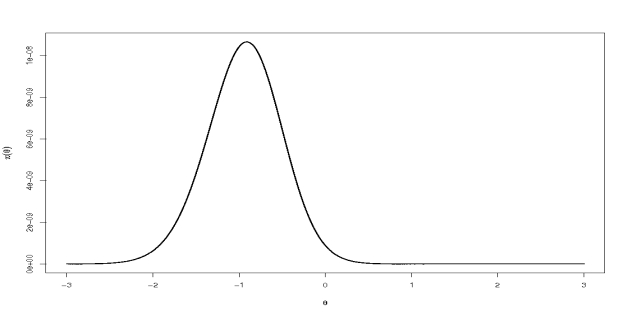
Consider a $t$-distribution $\mathcal{T}(\nu,\theta,1)$ sample $(x_{1},\ldots,x_{n})$ with $\nu$ known. Assume in addition a flat prior $\pi(\theta)=1$ as in a non-informative environment. While the posterior distribution on $\theta$ can be easily plotted, up to a normalising constant (Figure 1), because we are in dimension $1$, direct simulation and computation from this posterior is impossible.

Figure 1: Posterior density of $\theta$ in the setting of Example 8 for $n=10$, with a simulated sample from $\mathcal{T}(3,0,1)$.

If the inferential problem is to decide about the value of $\theta$, the posterior expectation is

$$\mathbb{E}^{\pi}[\theta|x_{1},\ldots,x_{n}]=\int\theta\prod_{i=1}^{n}\left[\nu+(x_{i}-\theta)^{2}\right]^{-(\nu+1)/2}\,\text{d}\theta$$

$$\qquad\bigg{/}\int\prod_{i=1}^{n}\left[\nu+(x_{i}-\theta)^{2}\right]^{-(\nu+1)/2}\,\text{d}\theta\,.$$

This ratio of integrals is not directly computable. Since $(\nu+(x_{i}-\theta)^{2})^{-(\nu+1)/2}$ is proportional to a $t$-distribution $\mathcal{T}(\nu,x_{i},1)$ density, a solution to the approximation of the integrals is to use one of the $i$’s to “be” the density in both integrals. For instance, if we generate $\theta_{1},\ldots,\theta_{m}$ from the $\mathcal{T}(\nu,x_{1},1)$ distribution, the equivalent of (5) is

$$\delta^{\pi}_{m} = \sum_{j=1}^{m}\theta_{j}\prod_{i=2}^{n}\left[\nu+(x_{i}-\theta_{j})^{2}\right]^{-(\nu+1)/2}$$

$$\qquad\bigg{/}\sum_{j=1}^{m}\prod_{i=2}^{n}\left[\nu+(x_{i}-\theta_{j})^{2}\right]^{-(\nu+1)/2}$$

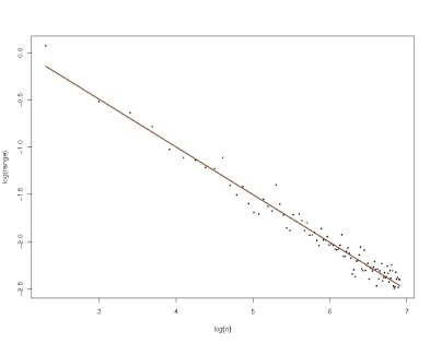
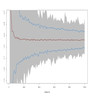
since the first term in the product has been “used” for the simulation and the normalisation constants have vanished in the ratio. Figure 2 is an illustration of the speed of convergence of this estimator to the true posterior expectation: it provides the evolution of $\delta^{\pi}_{m}$ as a function of $m$ both on average and on range (provided by repeated simulations of $\delta^{\pi}_{m}$). As can be seen from the graph, the average is almost constant from the start, as it should, because of unbiasedness, while the range decreases very slowly, as it should, because of extreme value theory. The graph provides in addition the $90$% empirical confidence interval built on these simulations. The empirical confidence intervals are decreasing in $1/\sqrt{n}$, as expected from the theory. (This is further established by regressing the log-lengths of the confidence intervals on $\log(n)$, with slope equal to $-0.5$, as shown by Figure 3.)

Figure 2: Evolution of a sequence of $500$ estimators (8) over $1,000$ iterations: range (in gray), $.05$ and $.95$ quantiles, and average, obtained on the same sample as in Figure 1 when simulating from the $t$ distribution with location $x_{1}$.

Figure 3: Regression of the log-ranges (left) and the log-lengths of the confidence intervals (right) on $\log(n)$, for the output in Figure 2.

Now, there is a clear arbitrariness in the choice of $x_{1}$ in the sample $(x_{1},\ldots,\allowbreak x_{n})$ for the proposal $\mathcal{T}(\nu,x_{1},1)$. While any of the $x_{i}$’s has the same theoretical validity to “represent” the integral and the integrating density, the choice of $x_{i}$’s closer to the posterior mode (the true value of $\theta$ is $0$) induces less variability in the estimates, as shown by a further simulation experiment through Figure 4. It is fairly clear from this comparison that the choice of extremal values like $x_{(1)}=-3.21$ and even more $x_{(10)}=1.72$ is detrimental to the quality of the approximation, compared with the median $x_{(5)}=-0.86$. The range of the estimators is much wider for both extremes, but the influence of this choice is also visible for the average which does not converge so quickly.

Figure 4: Repetition of the experiment described in Figure 2 for three different choices of $x_{i}$: $\min x_{i}$, $x_{(5)}$ and $\max x_{i}$ (from left to right).

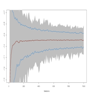
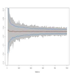
This example thus shows that Monte Carlo methods, while widely available, may easily face inefficiency problems when the simulated values are not sufficiently attuned to the distribution of interest. It also demonstrates that, fundamentally, there is no difference between importance sampling and regular Monte Carlo, in that the integral $\mathfrak{I}$ can naturally be represented in many ways.

Although we do not wish to spend too much space on this issue, let us note that the choice of the importance function gets paramount when the support of the function of interest is not the whole space. For instance, a tail probability, associated with $h(\theta)=\mathbb{I}_{\theta\geq\theta_{0}}$ say, should be estimated with an importance function whose support is $[\theta_{0},\infty)$. (See Robert and Casella, 2004, Chapter 3, for details.)

Example 9 (Continuation of Example 8)

If, instead, we wish to consider the probability that $\theta\geq 0$, using the $t$-distribution $\mathcal{T}(\nu,x_{i},1)$ is not a good idea because negative values of $\theta$ are somehow simulated “for nothing”. A better proposal (in terms of variance) is to use the “folded” $t$-distribution $\mathcal{T}(\nu,x_{i},1)$, with density proportional to

$$\psi_{i}(\theta)=\left[\nu+(x_{i}-\theta)^{2}\right]^{-(\nu+1)/2}+\left[\nu+(x_{i}+\theta)^{2}\right]^{-(\nu+1)/2}\,,$$

on $\mathbb{R}_{+}$, which can be simulated by taking the absolute value of a $\mathcal{T}(\nu,x_{i},1)$ rv. All simulated values are then positive and the estimator of the probability is

$$\rho^{\pi}_{m} = \sum_{j=1}^{m}\prod_{i\neq k}\left[\nu+(x_{i}-|\theta_{j}|)^{2}\right]^{-(\nu+1)/2}/\psi_{k}(|\theta_{j}|)$$

$$\qquad\bigg{/}\sum_{j=1}^{m}\prod_{i\neq k}\left[\nu+(x_{i}-\theta_{j})^{2}\right]^{-(\nu+1)/2}$$

where the $\theta_{j}$’s are iid $\mathcal{T}(\nu,x_{k},1)$. Note that this is a very special occurrence where the same sample can be used in both the numerator and the denominator. In fact, in most cases, two different samples have to be used, if only because the support of the importance distribution for the numerator is not the whole space, unless, of course, all normalising constants are known. Figure 5 reproduces earlier figures for this problem, when using $x_{(5)}$ as the parameter of the $t$ distribution.

Figure 5: Evolution of a sequence of $100$ estimators (9) over $1,000$ iterations (same legend as Figure 2).

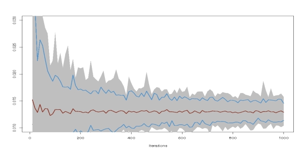
The above example is one-dimensional (in the parameter) and the problems exhibited there can be found severalfold in multidimensional settings. Indeed, while Monte Carlo methods do not suffer from the “curse of dimension” in the sense that the error of the corresponding estimators is always decreasing in $1/\sqrt{n}$, notwithstanding the dimension, it gets increasingly difficult to come up with satisfactory importance sampling distributions as the dimension gets higher and higher. As we will see in Section 0.5, the intuition built on MCMC methods has to be exploited to derive satisfactory importance functions.

Example 10 (Continuation of Example 2)

A particular case of generalised linear model is the probit model,

$$\hbox{Pr}_{\theta}(Y=1|x)=1-\hbox{Pr}_{\theta}(Y=0|x)=\Phi(x^{\mathrm{T}}\theta)\qquad\theta\in\mathbb{R}^{p}\,,$$

where $\Phi$ denotes the normal $\mathcal{N}(0,1)$ cdf. Under a flat prior $\pi(\theta)=1$, for a sample $(x_{1},y_{1}),\ldots,(x_{n},y_{n})$, the corresponding posterior distribution is proportional to

$$\prod_{i=1}^{n}\Phi(x_{i}^{\mathrm{T}}\theta)^{y_{i}}\Phi(-x_{i}^{\mathrm{T}}\theta)^{1-y_{i}}\,.$$ (8)

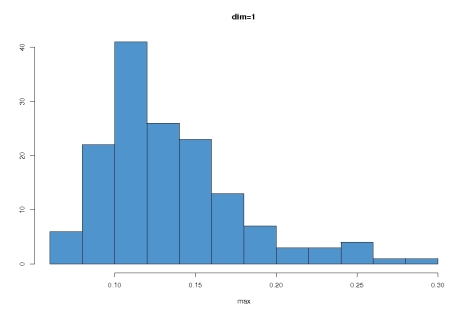
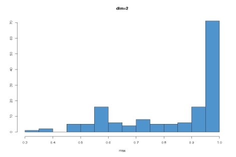
Direct simulation from this distribution is obviously impossible since the computation of $\Phi(z)$ is a difficulty in itself. If we pick an importance function for this problem, the adequation with the posterior distribution will need to be better and better as the dimension $p$ increases. Otherwise, the repartition of the weights will get increasingly asymmetric: very few weights will be different from $0$.

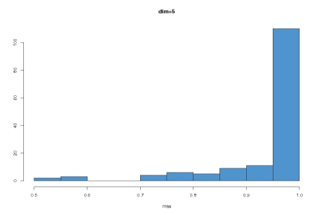
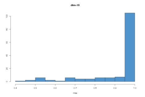
Figure 6 illustrates this degeneracy of the importance sampling approach as the dimension increases. We simulate parameters $\beta$’s and datasets $(x_{i},y_{i})$ $(i=1,\ldots,245)$ for dimensions $p$ ranging from $1$ to $10$, then represented the histograms of the largest weight for $p=1,2,5,10$. The $x_{i}$’s were simulated from a $\mathcal{N}_{p}(0,I_{p})$ distribution, while the importance sampling distribution was a $\mathcal{N}_{p}(0,I_{p}/p)$ distribution.

Figure 6: Comparison of the distribution of the largest importance weight based upon $150$ replications of an importance sampling experiment with $245$ observations and dimensions $p=1,2,5,10$.

0.3.3 Approximations of the Bayes factor

As explained in Sections 0.2.2 and 0.2.3, the first computational difficulty associated with Bayesian testing is the derivation of the Bayes factor, of the form

$$B^{\pi}_{12}=\dfrac{\displaystyle{\int_{\Theta_{1}}f_{1}(x|\theta_{1})\pi_{1}(\theta_{1})\text{d}\theta_{1}}}{\displaystyle{\int_{\Theta_{2}}f_{2}(x|\theta_{2})\pi_{2}(\theta_{2})\text{d}\theta_{2}}}=\frac{m_{1}(x)}{m_{2}(x)}\,,$$

where, for simplicity’s sake, we have adopted a model choice perspective (that is, $\theta_{1}$ and $\theta_{2}$ may live in completely different spaces).

Specific Monte Carlo methods for the estimation of ratios of normalising constants, or, equivalently, of Bayes factors, have been developed in the past five years. See Chen et al. (2000, Chapter 5) for a complete exposition, as well as Chopin and Robert (2010) and Marin and Robert (2007b) for recent reassessments. In particular, the importance sampling technique is rather well-adapted to the computation of those Bayes factors: Given a importance distribution, with density proportional to $g$, and a sample $\theta^{(1)},\ldots,\theta^{(T)}$ simulated from $g$, the marginal density for model $\mathfrak{M}_{i}$, $m_{i}(x)$, is approximated by

$$\widehat{m}_{i}(x)=\displaystyle{\sum_{t=1}^{T}f_{i}(x|\theta^{(t)})\dfrac{\pi_{i}(\theta^{(t)})}{g(\theta^{(t)})}}\bigg{/}\displaystyle{\sum_{t=1}^{T}\dfrac{\pi_{i}(\theta^{(t)})}{g(\theta^{(t)})}}\,,$$

where the denominator takes care of the (possibly) missing normalising constants. (Notice that, if $g$ is a density, the expectation of $\pi(\theta^{(t)})/g(\theta^{(t)})$ is $1$ and the denominator should be replaced by $T$ to decrease the variance of the estimator of $m_{i}(x)$.)

A compelling incentive, among others, for using importance sampling in the setting of model choice is that the sample $(\theta^{(1)},\ldots,\theta^{(T)})$ can be recycled for all models $\mathfrak{M}_{i}$ sharing the same parameters (in the sense that the models $\mathfrak{M}_{i}$ are parameterised in the same way, e.g. by their first moments).

Example 11 (Continuation of Example 4)

In the case the $\beta$’s are simulated from a product instrumental distribution

$$g(\beta)=\prod_{i=1}^{p}g_{i}(\beta_{i})\,,$$

the sample of $\beta$’s produced for the general model of Example 2, $\mathfrak{M}_{1}$ say, can also be used for the restricted model, $\mathfrak{M}_{2}$, where $\beta_{1}=0$, simply by deleting the first component and keeping the following components, with the corresponding importance density being

$$g_{-1}(\beta)=\prod_{i=2}^{p}g_{i}(\beta_{i})\,.$$

Once the $\beta$’s have been simulated, the Bayes factor $B^{\pi}_{12}$ can be approximated by $\widehat{m}_{1}(x)/\widehat{m}_{2}(x)$.

However, the variance of $\widehat{m}(x)$ may be infinite, depending on the choice of $g$. A possible choice is $g(\theta)=\pi(\theta)$, with wider tails than $\pi(\theta|x)$, but this is often inefficient if the data is informative because the prior and the posterior distributions will be quite different and most of the simulated values $\theta^{(t)}$ fall outside the modal region of the likelihood. (This is of course impossible when $\pi$ is improper.) For the choice $g(\theta)=f(x|\theta)\pi(\theta)$,

$$\widehat{m}(x)=1\bigg{/}\dfrac{1}{T}\sum_{t=1}^{T}\dfrac{1}{f(x|\theta^{(t)})}\,,$$ (9)

is the harmonic mean of the likelihoods, but the corresponding variance is infinite when the likelihood has thinner tails than the prior (which is often the case). Having an infinite variance means that the numerical value produced by the estimate cannot be trusted at all, as it may be away from the true marginal by several orders of magnitude. As discussed in Chopin and Robert (2010) and Marin and Robert (2007b), it is actually possible to use a generalised harmonic mean estimate

$$\widehat{m}(x)=1\bigg{/}\dfrac{1}{T}\sum_{t=1}^{T}\dfrac{\varphi(\theta^{(t)})}{\pi(\theta^{(t)})f(x|\theta^{(t)})}\,,$$

when $\varphi$ is a probability density with tails that are thinner than the posterior tails. For instance, a density with support an approximate HPD region is quite appropriate.

Explicitly oriented towards the computation of ratios of normalising constants, bridge sampling was introduced in Meng and Wong (1996): if both models $\mathfrak{M}_{1}$ and $\mathfrak{M}_{2}$ cover the same parameter space $\Theta$, if $\pi_{1}(\theta|x)=c_{1}{\tilde{\pi}}_{1}(\theta|x)$ and $\pi_{2}(\theta|x)=c_{2}{\tilde{\pi}}_{2}(\theta|x)$, where $c_{1}$ and $c_{2}$ are unknown normalising constants, then the equality

$$\frac{c_{2}}{c_{1}}=\frac{\mathbb{E}^{\pi_{2}}[{\tilde{\pi}}_{1}(\theta|x)\,h(\theta)]}{\mathbb{E}^{\pi_{1}}[{\tilde{\pi}}_{2}(\theta|x)\,h(\theta)]}$$

holds for any bridge function $h(\theta)$ such that both expectations are finite. The bridge sampling estimator is then

$$B^{S}_{12}=\dfrac{\displaystyle{\dfrac{1}{n_{1}}\sum_{i=1}^{n_{1}}{\tilde{\pi}}_{2}(\theta_{1i}|x)\,h(\theta_{1i})}}{\displaystyle{\dfrac{1}{n_{2}}\sum_{i=1}^{n_{2}}{\tilde{\pi}}_{1}(\theta_{2i}|x)\,h(\theta_{2i})}}\,,$$

where the $\theta_{ji}$’s are simulated from $\pi_{j}(\theta|x)$ $(j=1,2,\,i=1,\ldots,n_{j})$.

For instance, if

$$h(\theta)=1/\left[{\tilde{\pi}}_{1}(\theta|x){\tilde{\pi}}_{2}(\theta_{1i}|x)\right]\,,$$

then $B^{S}_{12}$ is a ratio of harmonic means, generalising (9). Meng and Wong (1996) have derived an (asymptotically) optimal bridge function

$$h^{*}(\theta)=\dfrac{n_{1}+n_{2}}{n_{1}\pi_{1}(\theta|x)+n_{2}\pi_{2}(\theta|x)}\,.$$

This choice is not of direct use, since the normalising constants of $\pi_{1}(\theta|x)$ and $\pi_{2}(\theta|x)$ are unknown (otherwise, we should not need to resort to such techniques!). Nonetheless, it shows that a good bridge function should cover the support of both posteriors, with equal weights if $n_{1}=n_{2}$.

Example 12 (Continuation of Example 2)

For generalised linear models, the mean (conditionally on the covariates) satisfies

$$\mathbb{E}[y|\theta]=\nabla\psi(\theta)=\Psi(x^{t}\beta)\,,$$

where $\Psi$ is the link function. The choice of the link function $\Psi$ usually is quite open. For instance, when the $y$’s take values in $\{0,1\}$, three common choices of $\Psi$ are (McCullagh and Nelder, 1989)

$$\Psi_{1}(t)=\exp(t)/(1+\exp(t)),\quad\Psi_{2}(t)=\Phi(t),\quad\hbox{and}\quad\Psi_{3}(t)=1-\exp(-\exp(t))\,,$$

corresponding to the logit, probit and log–log link functions (where $\Phi$ denotes the c.d.f. of the $\mathscr{N}(0,1)$ distribution). If the prior distribution $\pi$ on the $\beta$’s is a normal $\mathcal{N}_{p}(\xi,\tau^{2}I_{p})$, and if the bridge function is $h(\beta)=1/\pi(\beta)$, the bridge sampling estimate is then $(1\leq i<j\leq 3)$

$$B^{S}_{ij}=\dfrac{\displaystyle{\dfrac{1}{n}\sum_{t=1}^{n}f_{j}(\beta_{it}|x)}}{\displaystyle{\dfrac{1}{n}\sum_{t=1}^{n}f_{i}(\beta_{jt}|x)}}\,,$$

where the $\beta_{it}$ are generated from $\pi_{i}(\beta_{i}|x)\propto f_{i}(\beta_{i}|x)\pi(\beta_{i})$, that is, from the true posteriors for each link function.

The drawback in using bridge sampling is that the extension of the method to cases where the two models $\mathfrak{M}_{1}$ and $\mathfrak{M}_{2}$ do not cover the same parameter space, for instance because the two corresponding parameter spaces are of different dimensions, requires the introduction of a pseudo-posterior distribution (Chen et al., 2000; Marin and Robert, 2007b) that complete the smallest parameter space so that dimensions match. The impact of those completion pseudo-posteriors on the quality of the Bayes factor approximation is such that they cannot be suggested for a general usage in Bayes factor computation.

A completely different route to the approximation of a marginal likelihood is Chib’s (1995), which happens to be a direct application of Bayes’ theorem: given $x\sim f_{k}(x|\theta_{k})$ and $\theta_{k}\sim\pi_{k}(\theta_{k})$ $(k=1,2)$, we have that

$$m_{k}(x)=\frac{f_{k}(x|\theta)\,\pi_{k}(\theta)}{\pi_{k}(\theta|x)}\,,$$

for every value of $\theta$ (since both the lhs and the rhs of this equation are constant in $\theta$). Therefore, if an arbitrary value of $\theta$, say $\theta^{*}_{k}$, is selected—e.g., the MAP estimate—and if a good approximation to $\pi_{k}(\theta|y)$ can be constructed, denoted $\hat{\pi}(\theta|y)$, Chib’s (1995) approximation to the marginal likelihood $m_{k}(x)$ is

$$\widehat{m}_{k}(x)=\frac{f_{k}(y|\theta^{*}_{k})\,\pi_{k}(\theta^{*}_{k})}{\hat{\pi_{k}}(\theta^{*}_{k}|y)}\,.$$ (10)

As a first solution, $\hat{\pi}(\theta|y)$ may be a Gaussian approximation based on the MLE, but this is unlikely to be accurate in a general setting. Chib’s (1995) solution is to use a nonparametric approximation based on a preliminary Monte Carlo Markov chain (Section 0.4) sample, even though the accuracy may also suffer in large dimensions. In the special setting of latent variables models (like the mixtures of distributions discussed in Example 6), this approximation is particularly attractive as there exists a natural approximation to $\pi_{k}(\theta|y)$, based on the Rao–Blackwell (Gelfand and Smith, 1990) estimate

$$\hat{\pi_{k}}(\theta^{*}_{k}|y)=\frac{1}{T}\,\sum_{t=1}^{T}\pi_{k}(\theta^{*}_{k}|y,z_{k}^{(t)})\,,$$

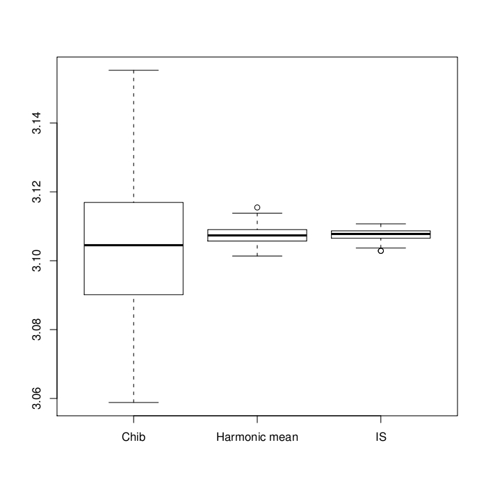
where the $z_{k}^{(t)}$’s are the latent variables simulated by the Monte Carlo Markov chain algorithm. The estimate $\hat{\pi_{k}}(\theta^{*}_{k}|y)$ is a parametric unbiased approximation of $\pi_{k}(\theta^{*}_{k}|y)$ that converges to the true density with rate $\text{O}(\sqrt{T})$. This Rao–Blackwell approximation obviously requires the full conditional density $\pi_{k}(\theta^{*}_{k}|y,z)$ to be available in closed form (constant included) but this is the case for many standard models. Figure 7 reproduces an illustration from Marin and Robert (2007b) that compares the variability of Chib’s (1995) method against nearly optimal harmonic and importance sampling approximations in the setting of a probit posterior distribution. While the former solution varies more than the two latter solutions, its generic features make Chib’s (1995) method a reference for this problem.

Figure 7: In the setting of the probit modelling of R Pima Indian dataset, using three covariates and testing for the significance of the diabetes pedigree function, boxplots of 100 Chib’s, harmonic mean and importance estimates of $B_{01}(y)$, based on simulations from the prior distributions, for $2\times 10^{4}$ simulations (Source: Marin and Robert, 2007b).

While amenable to an importance sampling technique of sorts, the alternative approach of nested sampling (Skilling, 2006) for computing evidence is discussed in Chopin and Robert (2010) and Robert and Wraith (2009). Similarly, the specific approach based on the Savage-Dickey (Dickey, 1971; Verdinelli and Wasserman, 1995) representation of the Bayes factor associated with the null hypothesis $H_{0}:\,\theta=\theta_{0}$, as

$$B_{01}(x)=\dfrac{\pi_{1}(\theta_{0}|x)}{\pi_{1}(\theta_{0})}\,,$$

can be related to the family of bridge sampling techniques, even though the initial theoretical foundations of the method are limited, as explained in Robert and Marin (2009). This paper engineered a general framework that produces a converging and unbiased approximation of the Bayes factor, unrelated with the approach of Verdinelli and Wasserman (1995), that builds upon a mixed pseudo-posterior naturally derived from the priors under both the null and the alternative hypotheses.

As can be seen from the previous developments, such methods require a rather careful tuning to be of any use. Therefore, they are rather difficult to employ outside settings where pairs of models are opposed. In other words, they cannot be directly used in general model choice settings where the parameter space (and in particular the parameter dimension) varies across models, as in, for instance, Example 7. To address the computational issues corresponding to these cases requires more advanced techniques introduced in the next Section.

0.4 Markov Chain Monte Carlo Methods

As described precisely in Chapter II.3 and in Robert and Casella (2004), MCMC methods try to overcome the limitation of regular Monte Carlo methods through the use of a Markov chain with stationary distribution the posterior distribution. There exist rather generic ways of producing such chains, including Metropolis–Hastings and Gibbs algorithms. Besides the fact that stationarity of the target distribution is enough to justify a simulation method by Markov chain generation, the idea at the core of MCMC algorithms is that local exploration, when properly weighted, can lead to a valid representation of the distribution of interest, as for instance, when using the Metropolis–Hastings algorithm.

0.4.1 Metropolis–Hastings as universal simulator

The Metropolis–Hastings, presented in Robert and Casella (2004) and Chapter II.3, offers a straightforward solution to the problem of simulating from the posterior distribution $\pi(\theta|x)\propto f(x|\theta)\,\pi(\theta)$: starting from an arbitrary point $\theta_{0}$, the corresponding Markov chain explores the surface of this posterior distribution by a similarly arbitrary random walk proposal $q(\theta|\theta^{\prime})$ that progressively visits the whole range of the possible values of $\theta$.

—Metropolis–Hastings Algorithm—

At iteration $t$ 1 Generate $\xi\sim q(\xi|\theta^{(t)})$, $u_{t}\sim\mathcal{U}([0,1])$ 2 Take $$\theta^{(t+1})=\begin{cases}\xi_{t}&\hbox{if }u_{t}\leq\displaystyle{\frac{\pi(\xi_{t}|x)}{\pi(\theta^{(t)}|x)}\frac{q(\theta^{(t)}|\xi_{t})}{q(\xi_{t}|\theta^{(t)})}}\cr\theta^{(t)}&\hbox{otherwise}\end{cases}$$

Example 13 (Continuation of Example 10)

In the case $p=1$, the probit model defined in Example 10 can also be over-parameterised as

$$\text{Pr}(Y_{i}=1|x_{i})=1-\text{Pr}(Y_{i}=0|x_{i})=\Phi(x_{i}\beta/\sigma)\,,$$

since it only depends on $\beta/\sigma$. The Bayesian processing of non-identified models poses no serious difficulty as long as the posterior distribution is well defined. This is the case for a proper prior like

$$\pi(\beta,\sigma^{2})\propto\sigma^{-4}\,\exp\{-1/\sigma^{2}\}\,\exp\{-\beta^{2}/50)$$

that corresponds to a normal distribution on $\beta$ and a gamma distribution on $\sigma^{-2}$. While the posterior distribution on $(\beta,\sigma)$ is not a standard distribution, it is available up to a normalising constant. Therefore, it can be directly processed via an MCMC algorithm. In this case, we chose a Gibbs sampler that simulates $\beta$ and $\sigma^{2}$ alternatively, from

$$\pi(\beta|\mathbf{x},\mathbf{y},\sigma)\propto\prod_{y_{i}=1}\Phi(x_{i}\beta/\sigma)\prod_{y_{i}=0}\Phi(-x_{i}\beta/\sigma)\times\pi(\beta)$$

and

$$\pi(\sigma^{2}|\mathbf{x},\mathbf{y},\beta)\propto\prod_{y_{i}=1}\Phi(x_{i}\beta/\sigma)\prod_{y_{i}=0}\Phi(-x_{i}\beta/\sigma)\times\pi(\sigma^{2})$$

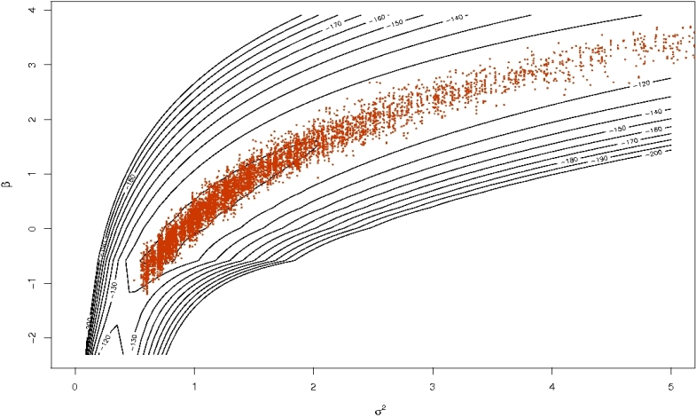
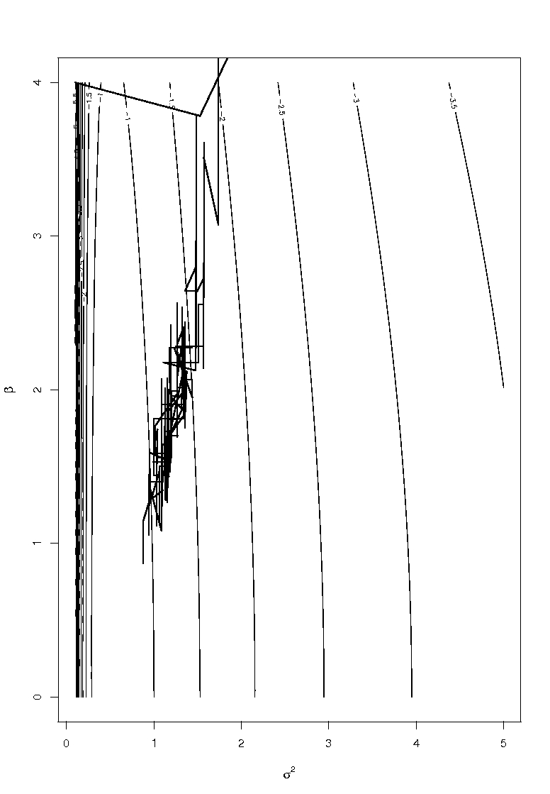
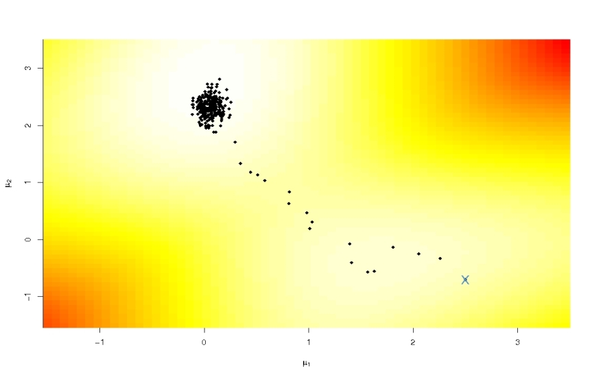
respectively. Since both of these conditional distributions are also non-standard, we replace the direct simulation by a one-dimensional Metropolis–Hastings step, using normal $\mathcal{N}(\beta^{(t)},1)$ and log-normal $\mathcal{L}\mathcal{N}(\log\sigma^{(t)},.04)$ random walk proposals, respectively. For a simulated dataset of $1,000$ points, the contour plot of the log-posterior distribution is given in Figure 8, along with the last $1,000$ points of a corresponding MCMC sample after $100,000$ iterations. This graph shows a very satisfactory repartition of the simulated parameters over the likelihood surface, with higher concentrations near the largest posterior regions. For another simulation, Figure 9 details the first $500$ steps, when started at $(\beta,\sigma^{2})=(0.1,4.0)$. Although each step contains both a $\beta$ and a $\sigma$ proposal, some moves are either horizontal or vertical: this corresponds to cases when either the $\beta$ or the $\sigma$ proposals have been rejected. Note also the fairly rapid convergence to a modal zone of the posterior distribution in this case.

Figure 8: Contour plot of the log-posterior distribution for a probit sample of $1,000$ observations, along with $1,000$ points of an MCMC sample (Source: Robert and Casella, 2004).

Figure 9: First $500$ steps of the Metropolis–Hastings algorithm on the probit log-posterior surface, when started at $(\beta,\sigma^{2})=(0.1,4.0)$.

Obviously, this is only a toy example and more realistic probit models do not fare so well with down-the-shelf random walk Metropolis–Hastings algorithms, as shown for instance in Nobile (1998) (see also Robert and Casella, 2004, Section 10.3.2, Marin and Robert, 2007a, Section 4.3, and Marin and Robert, 2007b).

The difficulty inherent to random walk Metropolis–Hastings algorithms is the scaling of the proposal distribution: it must be adapted to the shape of the target distribution so that, in a reasonable number of steps, the whole support of this distribution can be visited. If the scale of the proposal is too small, this will not happen as the algorithm stays “too local” and, if there are several modes on the posterior, the algorithm may get trapped within one modal region because it cannot reach other modal regions with jumps of too small a magnitude. The larger the dimension $p$ is, the harder it is to set up the right scale, though, because

1. the curse of dimension implies that there are more and more empty regions in the space, that is, regions with zero posterior probability;

2. the knowledge and intuition about the modal regions get weaker and weaker;

3. the proper scaling involves a symmetric $(p,p)$ matrix $\Xi$ in the proposal $g((\theta-\theta^{\prime})^{\mathrm{T}}\Xi(\theta-\theta^{\prime}))$. Even when the matrix $\Xi$ is diagonal, it gets harder to scale as the dimension increases (unless one resorts to a Gibbs like implementation, where each direction is scaled separately).

Note also that the on-line scaling of the algorithm against the empirical acceptance rate is inherently flawed in that (a) the process is no longer Markovian and (b) the attraction of a modal region may give a false sense of convergence and lead to a choice of too small a scale, simply because other modes will not be visited during the scaling experiment.

0.4.2 Gibbs sampling and latent variable models

The Gibbs sampler is a definitely attractive algorithm for Bayesian problems because it naturally fits the hierarchical structures so often found in such problems. “Natural” being a rather vague notion from a simulation point of view, it routinely happens that other algorithms fare better than the Gibbs sampler. Nonetheless, Gibbs sampler is often worth a try (possibly with other Metropolis–Hastings refinements at a later stage) in well-structured objects like Bayesian hierarchical models and more general graphical models.

A very relevant illustration is made of latent variable models, where the observational model is itself defined as a mixture model,

$$f(x|\theta)=\int_{\mathscr{Z}}f(x|z,\theta)\,g(z|\theta)\,\text{d}z.$$

Such models were instrumental in promoting the Gibbs sampler in the sense that they have the potential to make Gibbs sampling sound natural very easily. (See also Chapter II.3.) For instance, Tanner and Wong (1987) wrote a precursor article to Gelfand and Smith (1990) that designed specific two-stage Gibbs samplers for a variety of latent variable models. And many of the first applications of Gibbs sampling in the early 90’s were actually for models of that kind. The usual implementation of the Gibbs sampler in this case is to simulate the missing variables $Z$ conditional on the parameters and reciprocally, as follows:

—Latent Variable Gibbs Algorithm—

At iteration $t$ 1 Generate $z^{(t+1)}\sim g(z|\theta^{(t)},x)$ 2 Generate $\theta^{(t+1)}\sim\pi(\theta|x,z^{(t+1)})$

While we could have used the probit case as an illustration (Example 10), as done in Chapter II.3, we choose to pick the case of mixtures (Example 6) as a better setting.

Example 14 (Continuation of Example 6)

The natural missing data structure of a mixture of distribution is historical. In one of the first mixtures to be ever studied by Bertillon, in 1863, a bimodal structure on the height of conscripts in south eastern France (Doubs) can be explained by the mixing of two populations of military conscripts, one from the plains and one from the mountains (or hills). Therefore, in the analysis of data from distributions of the form

$$\sum_{i=1}^{k}p_{i}f(x|\theta_{i})\,,$$

a common missing data representation is to associate with each observation $x_{j}$ a missing multinomial variable $z_{j}\sim\mathcal{M}_{k}(1;p_{1},\ldots,p_{k})$ such that $x_{j}|z_{j}=i\sim f(x|\theta_{i})$. In heterogeneous populations made of several homogeneous subgroups or subpopulations, it makes sense to interpret $z_{j}$ as the index of the population of origin of $x_{j}$, which has been lost in the observational process.

However, mixtures are also customarily used for density approximations, as a limited dimension proxy to non-parametric approaches. In such cases, the components of the mixture and even the number $k$ of components in the mixture are often meaningless for the problem to be analysed. But this distinction between natural and artificial completion (by the $z_{j}$’s) is lost to the MCMC sampler, whose goal is simply to provide a Markov chain that converges to the posterior as stationary distribution. Completion is thus, from a simulation point of view, a mean to generate such a chain.

The most standard Gibbs sampler for mixture models (Diebolt and Robert, 1994) is thus based on the successive simulation of the $z_{j}$’s and of the $\theta_{i}$’s, conditional on one another and on the data:

1. Generate $z_{j}|\theta,x_{j}$ $(j=1,\ldots,n)$

2. Generate $\theta_{i}|\mathbf{x},\mathbf{z}$ $(i=1,\ldots,k)$

Given that the density $f$ is most often from an exponential family, the simulation of the $\theta_{i}$’s is generally straightforward.

As an illustration, consider the (academic) case of a normal mixture with two components, with equal known variance and fixed weights,

$$p\,\mathcal{N}(\mu_{1},\sigma^{2})+(1-p)\,\mathcal{N}(\mu_{2},\sigma^{2})\,.$$ (11)

Assume in addition a normal $\mathcal{N}(0,10\sigma^{2})$ prior on both means $\mu_{1}$ and $\mu_{2}$. It is easy to see that $\mu_{1}$ and $\mu_{2}$ are independent, given $(\mathbf{z},\mathbf{x})$, and the respective conditional distributions are

$$\mathcal{N}\left(\sum_{z_{i}=j}x_{i}/\left(.1+n_{j}\right),\sigma^{2}/\left(.1+n_{j}\right)\right)\,,$$

where $n_{j}$ denotes the number of $z_{i}$’s equal to $j$. Even more easily, it comes that the conditional posterior distribution of $\mathbf{z}$ given $(\mu_{1},\mu_{2})$ is a product of binomials, with

$$\text{Pr}(Z_{i}=1|x_{i},\mu_{1},\mu_{2})$$

$$= \frac{p\exp\{-(x_{i}-\mu_{1})^{2}/2\sigma^{2}\}}{p\exp\{-(x_{i}-\mu_{1})^{2}/2\sigma^{2}\}+(1-p)\exp\{-(x_{i}-\mu_{2})^{2}/2\sigma^{2}\}}\,.$$

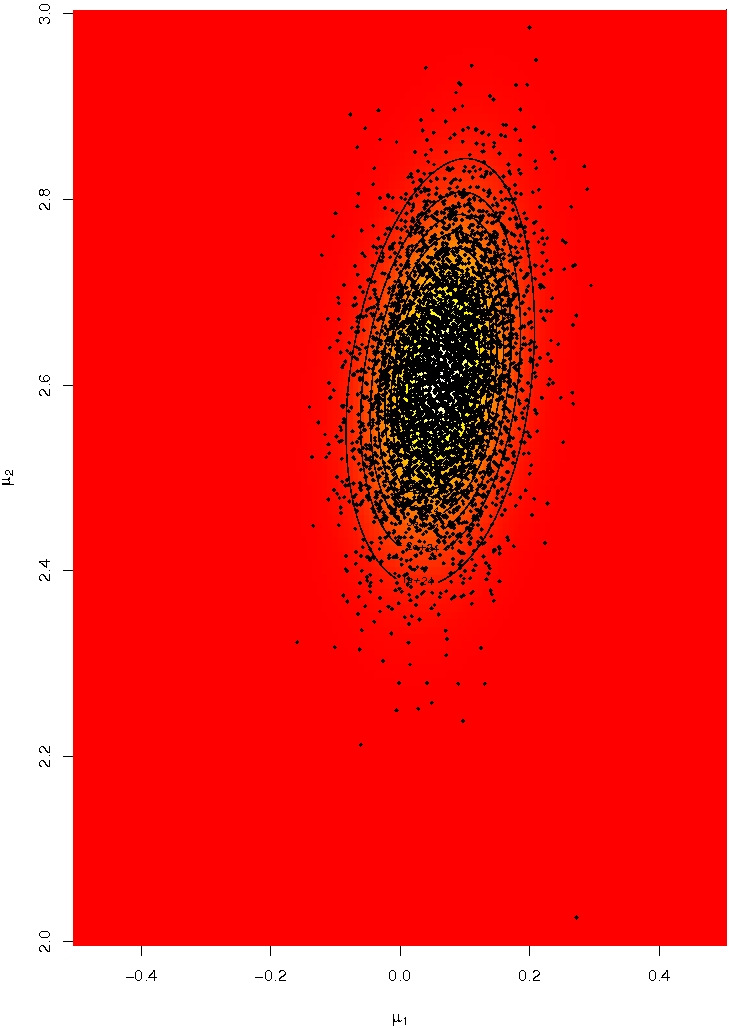
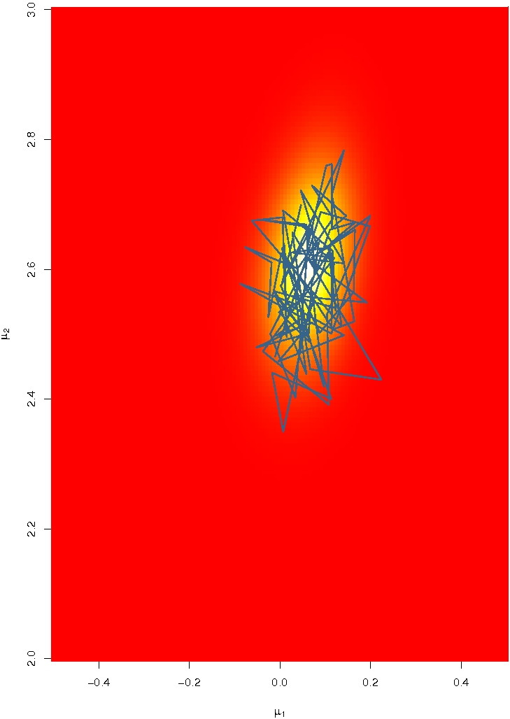
Figure 10 illustrates the behaviour of the Gibbs sampler in that setting, with a simulated dataset of $100$ points from the $.7\mathcal{N}(0,1)+.3\mathcal{N}(2.7,1)$ distribution. The representation of the MCMC sample after $5,000$ iterations is quite in agreement with the posterior surface, represented via a grid on the $(\mu_{1},\mu_{2})$ space and some contours. The sequence of consecutive steps represented on the left graph also shows that the mixing behaviour is satisfactory, since the jumps are scaled in terms of the modal region of the posterior.

Figure 10: Gibbs sample of $5,000$ points for the mixture posterior (left) and path of the last $100$ consecutive steps (right) against the posterior surface (Source: Robert and Casella, 2004).

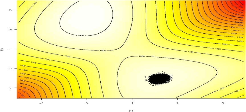
This experiment gives a wrong sense of safety, though, because it does not point out the fairly large dependence of the Gibbs sampler to the initial conditions, already signalled in Diebolt and Robert (1994) under the name of trapping states. Indeed, the conditioning of $(\mu_{1},\mu_{2})$ on $\mathbf{z}$ implies that the new simulations of the means will remain very close to the previous values, especially if there are many observations, and thus that the new allocations $\mathbf{z}$ will not differ much from the previous allocations. In other words, to see a significant modification of the allocations (and thus of the means) would require a very very large number of iterations. Figure 11 illustrates this phenomenon for the same sample as in Figure 10, for a wider scale: there always exists a second mode in the posterior distribution, which is much lower than the first mode located around $(0,2.7)$. Nonetheless, a Gibbs sampler initialised close to the second and lower mode will not be able to leave the vicinity of this (irrelevant) mode, even after a large number of iterations. The reason is as given above: to jump to the other mode, a majority of $z_{j}$’s would need to change simultaneously and the probability of such a jump is too close to $0$ to let the event occur.

Figure 11: Posterior surface and corresponding Gibbs sample for the two mean mixture model, when initialised close to the second and lower mode, based on $10,000$ iterations (Source: Robert and Casella, 2004).

The literature on this specific issue—of exploring all the modes of the posterior distribution—has grown around the denomination of “label switching problem”. For instance, Celeux et al. (2000) have pointed out the deficiency of most MCMC samplers in this respect, while Frühwirth-Schnatter (2001, 2004, 2006), Berkhof et al. (2003), Jasra et al. (2005), and Geweke (2007) have proposed different devices to overcome this difficulty, in particular when testing for the number of components. See Lee et al. (2009) for a survey on recent developments.

This example illustrates quite convincingly that, while the completion is natural from a model point of view (since it is a part of the definition of the model), it does not necessarily transfer its utility for the simulation of the posterior. Actually, when the missing variable model allows for a closed form likelihood, as is the case for mixtures, probit models (Examples 10 and 13) and even hidden Markov models (see Cappé et al., 2005), the whole range of the MCMC technology can be used as well. The appeal of alternatives like random walk Metropolis–Hastings schemes is that they remain in a smaller dimension space, since they avoid the completion step(s), and that they are not restricted in the range of their moves.

Example 15 (Continuation of Example 14)

Given that the likelihood of a sample $(x_{1},\ldots,x_{n})$ from the mixture distribution (11) can be computed in $\hbox{O}(2n)$ time, a regular random walk Metropolis–Hastings algorithm can be used in this setup. Figure 12 shows how quickly this algorithm escapes the attraction of the poor mode, as opposed to the Gibbs sampler of Figure 11: within a few iterations of the algorithm, the chain drifts over the poor mode and converges almost deterministically to the proper region of the posterior surface. The random walk is based on $\mathcal{N}(\mu_{i}^{(t)},0.04)$ proposals, although other scales would work as well but would require more iterations to reach the proper model regions. For instance, a scale of $0.005$ in the Normal proposal above needs close to $5,000$ iterations to attain the main mode.

Figure 12: Track of a $1,000$ iteration random walk Metropolis–Hastings chain on the posterior surface, the starting point being indicated by a cross. (The scale of the random walk is $0.2$.)

The secret of a successful MCMC implementation in such latent variable models is to maintain the distinction between latency in models and latency in simulation (the later being often called use of auxiliary variables). When latent variables can be used with adequate mixing of the resulting chain and when the likelihood cannot be computed in a closed form (as in hidden semi-Markov models, Cappé et al., 2004), a Gibbs sampler is a rather simple solution that is often easy to simulate from. Adding well-mixing random walk Metropolis–Hastings steps in the simulation scheme cannot hurt the overall mixing of the chain (Robert and Casella, 2004, Chap. 13), especially when several scales can be used at once (see Section 0.5). Note also that the technique of tempering that flattens the target distribution in order to facilitate its exploration by a Markov chain is available for most latent variable models, if sometimes in rudimentary versions. See Chopin (2007) and Marin and Robert (2007, Section 6.6) for an illustration in the setups of hidden Markov models and of mixtures (Example 15), respectively. A final word is that the latent variable completion can be conducted in an infinity of ways and that several of these should be tried or used in parallel to increase the chances of success.

0.4.3 Reversible jump algorithms for variable dimension models

As described in Section 0.2.3, model choice is computationally different from testing in that it considers at once a (much) wider range of models $\mathfrak{M}_{i}$ and parameter spaces $\Theta_{i}$. Although early approaches could only go through a pedestrian pairwise comparison, a more adequate perspective is to envision the model index $\mu$ as part of the parameter to be estimated, as in (3). The (computational) difficulty is that we are then dealing with a possibly infinite space that is the collection of unrelated sets: how can we then simulate from the corresponding distribution?

The MCMC solution proposed by Green (1995) is called reversible jump MCMC, because it is based on a reversibility constraint on the transitions between the sets $\Theta_{i}$. In fact, the only real difficulty compared with previous developments is to validate moves (or jumps) between the $\Theta_{i}$’s, since proposals restricted to a given $\Theta_{i}$ follow from the usual (fixed-dimensional) theory. Furthermore, reversibility can be processed at a local level: since the model indicator $\mu$ is a integer-valued random variable, we can impose reversibility for each pair $(k_{1},k_{2})$ of possible values of $\mu$. The idea at the core of reversible jump MCMC is then to supplement each of the spaces $\Theta_{k_{1}}$ and $\Theta_{k_{2}}$ with adequate artificial spaces in order to create a bijection between them. For instance, if $\dim(\Theta_{k_{1}})>\dim(\Theta_{k_{2}})$ and if the move from ${\Theta}_{k_{1}}$ to ${\Theta}_{k_{2}}$ can be represented by a deterministic transformation of $\theta^{(k_{1})}$

$$\theta^{(k_{2})}=T_{k_{1}\rightarrow k_{2}}(\theta^{(k_{1})})\,,$$

Green (1995) imposes a dimension matching condition which is that the opposite move from ${\Theta}_{k_{2}}$ to ${\Theta}_{k_{1}}$ is concentrated on the curve

$$\left\{\theta^{(k_{1})}\,:\,\theta^{(k_{2})}=T_{k_{1}\rightarrow k_{2}}(\theta^{(k_{1})})\right\}\;.$$

In the general case, if $\theta^{(k_{1})}$ is completed by a simulation $u_{k_{1}}\sim g_{k_{1}}(u_{k_{1}})$ into $(\theta^{(k_{1})},\allowbreak u_{k_{1}})$ and $\theta^{(k_{2})}$ by $u_{k_{2}}\sim g_{k_{2}}(u_{k_{2}})$ into $(\theta^{(k_{2})},\allowbreak u_{k_{2}})$ so that the mapping between $(\theta^{(k_{1})},u_{k_{1}})$ and $(\theta^{(k_{2})},u_{k_{2}})$ is a bijection,

$$(\theta^{(k_{2})},u_{k_{2}})=T_{k_{1}\rightarrow k_{2}}(\theta^{(k_{1})},u_{k_{1}}),$$ (12)

the probability of acceptance for the move from model ${\mathfrak{M}}_{k_{1}}$ to model ${\mathfrak{M}}_{k_{2}}$ is then

$$\min\left(\dfrac{\pi(k_{2},\theta^{(k_{2})})}{\pi(k_{1},\theta^{(k_{1})})}\;\dfrac{\pi_{21}g_{k_{2}}(u_{k_{2}})}{\pi_{12}g_{k_{1}}(u_{k_{1}})}\;\left|\dfrac{\partial T_{k_{1}\rightarrow k_{2}}(\theta^{(k_{1})},u_{k_{1}})}{\partial(\theta^{(k_{1})},u_{k_{1}})}\right|,1\right)\;,$$

involving

• the Jacobian of the transform $T_{k_{1}\rightarrow k_{2}}$,,

• the probability $\pi_{ij}$ of choosing a jump to ${\cal M}_{k_{j}}$ while in ${\cal M}_{k_{i}}$, and

• $g_{i}$, the density of $u_{i}$.

The acceptance probability for the reverse move is based on the inverse ratio if the move from ${\mathfrak{M}}_{k_{2}}$ to ${\mathfrak{M}}_{k_{1}}$ also satisfies (12) with $u_{k_{2}}\sim g_{k_{2}}(u_{k_{2}})$.

The pseudo-code representation of Green’s algorithm is thus as follows:

—Green’s Algorithm—

At iteration $t$, if $x^{(t)}=(m,\theta^{(m)})$, 1. Select model ${\mathfrak{M}}_{n}$ with probability $\pi_{mn}$ 2. Generate $u_{mn}\sim\varphi_{mn}(u)$ 3. Set $(\theta^{(n)},v_{nm})=T_{m\rightarrow n}(\theta^{(m)},u_{mn})$ 4. Take $x^{(t+1)}=(n,\theta^{(n)})$ with probability $$\min\left(\dfrac{\pi(n,\theta^{(n)})}{\pi(m,\theta^{(m)})}\;\dfrac{\pi_{nm}\varphi_{nm}(v_{nm})}{\pi_{mn}\varphi_{mn}(u_{mn})}\;\left|\dfrac{\partial T_{m\rightarrow n}(\theta^{(m)},u_{mn})}{\partial(\theta^{(m)},u_{mn})}\right|,1\right)\;,$$ and take $x^{(t+1)}=x^{(t)}$ otherwise.

Even more than previous methods, the implementation of this algorithm requires a high degree of skillfulness in picking the right proposals and the appropriate scales. Indeed, it may be argued that the ultimate dependence of the method on the pairwise completion schemes prevents an extension of its use by a broader audience. This “art of reversible jump MCMC” is illustrated on the two following examples, extracted from Robert and Casella (2004, Section 14.2.3).

Example 16 (Continuation of Example 6)

If we consider for model ${\mathfrak{M}}_{k}$ the $k$ component normal mixture distribution,

$$\sum_{j=1}^{k}p_{jk}{\cal N}(\mu_{jk},\sigma_{jk}^{2})\,,$$

moves between models involve changing the number of components in the mixture and thus adding new components or removing older components or yet again changing several components. As in Richardson and Green (1997), we can restrict the moves when in model ${\mathfrak{M}}_{k}$ to only models ${\mathfrak{M}}_{k+1}$ and ${\mathfrak{M}}_{k-1}$. The simplest solution is to use a birth-and-death process: The birth step consists in adding a new normal component in the mixture generated from the prior and the death step is the opposite, removing one of the $k$ components at random. In this case, the corresponding birth acceptance probability is

$$\min\left(\frac{\pi_{(k+1)k}}{\pi_{k(k+1)}}\,\frac{(k+1)!}{k!}\frac{\pi_{k+1}(\theta_{k+1})}{\pi_{k}(\theta_{k})\,(k+1)\varphi_{k(k+1)}(u_{k(k+1)})}\,,1\right)$$

$$\quad=\min\left(\frac{\pi_{(k+1)k}}{\pi_{k(k+1)}}\,\frac{\varrho(k+1)}{\varrho(k)}\,\frac{\ell_{k+1}(\theta_{k+1})\,(1-p_{k+1})^{k-1}}{\ell_{k}(\theta_{k})},1\right)\,,$$

where $\ell_{k}$ denotes the likelihood of the $k$ component mixture model ${\mathfrak{M}}_{k}$ and $\varrho(k)$ is the prior probability of model ${\mathfrak{M}}_{k}$.

While this proposal can work well in some setting, as in Richardson and Green (1997) when the prior is calibrated against the data, it can also be inefficient, that is, leading to a high rejection rate, if the prior is vague, since the birth proposals are not tuned properly. A second proposal, central to the solution of Richardson and Green (1997), is to devise more local jumps between models, called split and combine moves, since a new component is created by splitting an existing component into two, under some moment preservation conditions, and the reverse move consists in combining two existing components into one, with symmetric constraints that ensure reversibility. (See, e.g., Robert and Casella, 2004, for details.)

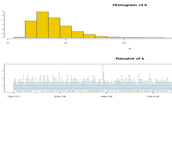
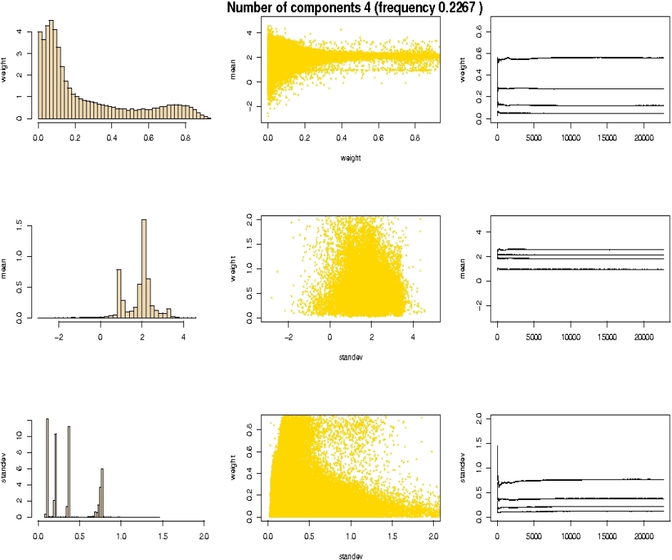
Figures 13–15 illustrate the implementation of this algorithm for the so-called Galaxy dataset used by Richardson and Green (1997) (see also Roeder, 1992), which contains $82$ observations on the speed of galaxies. On Figure 13, the MCMC output on the number of components $k$ is represented as a histogram on $k$, and the corresponding sequence of $k$’s. The prior used on $k$ is a uniform distribution on $\{1,\ldots,20\}$: as shown by the lower plot, most values of $k$ are explored by the reversible jump algorithm, but the upper bound does not appear to be restrictive since the $k^{(t)}$’s hardly ever reach this upper limit. Figure 14 illustrates the fact that conditioning the output on the most likely value of $k$ ($3$ here) is possible. The nine graphs in this Figure show the joint variation of the three types of parameters, as well as the stability of the Markov chain over the $1,000,000$ iterations: the cumulated averages are quite stable, almost from the start.

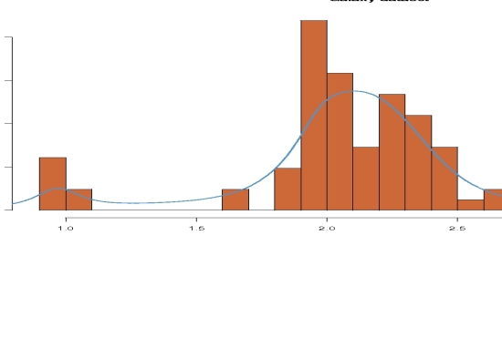
The density plotted on top of the histogram in Figure 15 is another good illustration of the inferential possibilities offered by reversible jump algorithms, as a case of model averaging: this density is obtained as the average over iterations $t$ of

$$\sum_{j=1}^{k^{(t)}}p^{(t)}_{jk}{\cal N}(\mu^{(t)}_{jk},(\sigma^{(t)}_{jk})^{2})\,,$$

which approximates the posterior expectation $\mathbb{E}[f(y|\theta)|\mathbf{x}]$, where $\mathbf{x}$ denotes the data $x_{1},\ldots,x_{82}$.

Figure 13: Histogram and raw plot of $100,000$ $k$’s produced by a reversible jump MCMC algorithm for the Galaxy dataset.

Figure 14: Reversible jump MCMC output on the parameters of the model ${\cal M}_{3}$ for the Galaxy dataset, obtained by conditioning on $k=3$. The left column gives the histogram of the weights, means, and variances; the middle column the scatterplot of the pairs weights-means, means-variances, and variances-weights; the right column plots the cumulated averages (over iterations) for the weights, means, and variances.

Figure 15: Fit of the dataset by the averaged density, $\mathbb{E}[f(y|\theta)|\mathbf{x}]$

Example 17 (Continuation of Example 3)

For the $AR(p)$ model of Example 3, the best way to include the stationarity constraints is to use the lag-polynomial representation

$$\prod_{i=1}^{p}\left(1-\lambda_{i}B\right)\,X_{t}=\epsilon_{t}\,,\quad\epsilon_{t}\sim{\mathcal{N}}(0,\sigma^{2})\,,$$

of model ${\mathfrak{M}}_{p}$, and to constrain the inverse roots, $\lambda_{i}$, to stay within the unit circle if complex and within $[-1,1]$ if real (see, e.g. Robert, 2007, Section 4.5.2). The associated uniform priors for the real and complex roots $\lambda_{j}$ is

$$\pi_{p}(\boldsymbol{\lambda})=\frac{1}{\lfloor p/2\rfloor+1}\,\prod_{\lambda_{i}\in{\mathbb{R}}}\frac{1}{2}{\mathbb{I}}_{|\lambda_{i}|<1}\,\prod_{\lambda_{i}\not\in{\mathbb{R}}}\frac{1}{\pi}{\mathbb{I}}_{|\lambda_{i}|<1}\,,$$

where $\lfloor p/2\rfloor+1$ is the number of different values of $r_{p}$. This factor must be included within the posterior distribution when using reversible jump since it does not vanish in the acceptance probability of a move between models ${\mathfrak{M}}_{p}$ and ${\mathfrak{M}}_{q}$. Otherwise, this results in a modification of the prior probability of each model.

Once again, a simple choice is to use a birth-and-death scheme where the birth moves either create a real or two conjugate complex roots. As in the birth-and-death proposal for Example 16, the acceptance probability simplifies quite dramatically since it is for instance

$$\min\left(\frac{\pi_{(p+1)p}}{\pi_{p(p+1)}}\,\frac{(r_{p}+1)!}{r_{p}!}\,\frac{\lfloor p/2\rfloor+1}{\lfloor(p+1)/2\rfloor+1}\frac{\ell_{p+1}(\theta_{p+1})}{\ell_{p}(\theta_{p})},1\right)$$

in the case of a move from ${\mathfrak{M}}_{p}$ to ${\mathfrak{M}}_{p+1}$. (As for the above mixture example, the factorials are related to the possible choices of the created and the deleted roots.)

Figure 16: Output of a reversible jump algorithm based on an $AR(3)$ simulated dataset of 530 points (upper left) with true parameters $\theta_{i}$ $(-0.1,0.3,-0.4)$ and $\sigma=1$. The first histogram is associated with $k$, the following histograms are associated with the $\theta_{i}$’s, for different values of $k$, and of $\sigma^{2}$. The final graph is a scatterplot of the complex roots (for iterations where there were complex roots). The one before last graph plots the evolution over the iterations of $\theta_{1},\theta_{2},\theta_{3}$ (Source: Robert 2003).

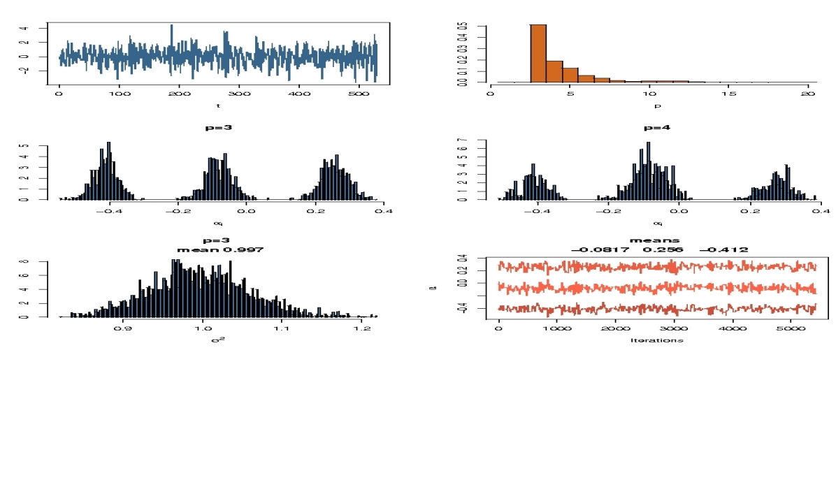
Figure 16 presents some views of the corresponding reversible jump MCMC algorithm. Besides the ability of the algorithm to explore a range of values of $k$, it also shows that Bayesian inference using these tools is much richer, since it can, for instance, condition on or average over the order $k$, mix the parameters of different models and run various tests on these parameters. A last remark on this graph is that both the order and the value of the parameters are well estimated, with a characteristic trimodality on the histograms of the $\theta_{i}$’s, even when conditioning on $k$ different from $3$, the value used for the simulation.

In conclusion, while reversible jump MCMC is a generic and powerful method for handling model comparison when faced with a multitude of models, its sensitivity to the tuning “parameters” that determine the pairwise jumps makes us favour the alternative of computing Bayes factors. When the number of models under comparisons is sufficiently small to allow for the computation of all marginal likelihoods in parallel, this computational solution is more efficient. It is indeed quite rare that the structure of the posterior under a model $\mathfrak{M}_{1}$ provides information about the structure of the posterior under another model $\mathfrak{M}_{2}$, unless both models are quite close. Intrinsically, reversible jump MCMC is a random walk over the collection of models and, as such, looses in efficiency in its exploration of this collection. (In particular, it almost never makes sense to implement reversible jump MCMC when comparing a small number of models.)

0.5 More Monte Carlo Methods

While MCMC algorithms considerably expanded the range of applications of Bayesian analysis, they are not, by any means, the end of the story! Further developments are taking place, either at the fringe of the MCMC realm or far away from it. We indicate below a few of the directions in Bayesian computational Statistics, omitting many more that also are of interest…

0.5.1 Adaptivity for MCMC algorithms

Given the range of situations where MCMC applies, it is unrealistic to hope for a generic MCMC sampler that would function in every possible setting. The more generic proposals like random-walk Metropolis–Hastings algorithms are known to fail in large dimension and disconnected supports, because they take too long to explore the space of interest (Neal, 2003). The reason for this impossibility theorem is that, in realistic problems, the complexity of the distribution to simulation is the very reason why MCMC is used! So it is difficult to ask for a prior opinion about this distribution, its support or the parameters of the proposal distribution used in the MCMC algorithm: intuition is close to void in most of these problems.

However, the performances of off-the-shelve algorithms like the random-walk Metropolis–Hastings scheme bring information about the distribution of interest and, as such, should be incorporated in the design of better and more powerful algorithms. The problem is that we usually miss the time to train the algorithm on these previous performances and are looking for the Holy Grail of automated MCMC procedures! While it is natural to think that the information brought by the first steps of an MCMC algorithm should be used in later steps, there is a severe catch: using the whole past of the “chain” implies that this is not a Markov chain any longer. Therefore, usual convergence theorems do not apply and the validity of the corresponding algorithms is questionable. Further, it may be that, in practice, such algorithms do degenerate to point masses because of a too rapid decrease in the variation of their proposal.

Example 18 (Continuation of Example 8)

For the $t$-distribution sample, we could fit a normal proposal from the empirical mean and variance of the previous values of the chain,

$$\mu_{t}=\frac{1}{t}\,\sum_{i=1}^{t}\theta^{(i)}\quad\hbox{and}\quad\sigma^{2}_{t}=\frac{1}{t}\,\sum_{i=1}^{t}(\theta^{(i)}-\mu_{t})^{2}\,.$$

This leads to a Metropolis–Hastings algorithm with acceptance probability

$$\prod_{j=2}^{n}\left[\frac{\nu+(x_{j}-\theta^{(t)})^{2}}{\nu+(x_{j}-\xi)^{2}}\right]^{-(\nu+1)/2}\,\frac{\exp-(\mu_{t}-\theta^{(t)})^{2}/2\sigma^{2}_{t}}{\exp-(\mu_{t}-\xi)^{2}/2\sigma^{2}_{t}}\,,$$

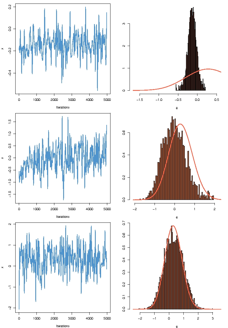
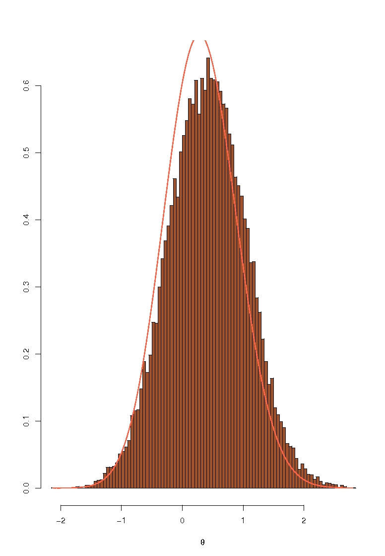
where $\xi$ is the proposed value from $\mathcal{N}(\mu_{t},\sigma^{2}_{t})$. The invalidity of this scheme (because of the dependence on the whole sequence of $\theta^{(i)}$’s till iteration $t$) is illustrated in Figure 17: when the range of the initial values is too small, the sequence of $\theta^{(i)}$’s cannot converge to the target distribution and concentrates on too small a support. But the problem is deeper, because even when the range of the simulated values is correct, the (long-term) dependence on past values modifies the distribution of the sequence. Figure 18 shows that, for an initial variance of $2.5$, there is a bias in the histogram, even after $25,000$ iterations and stabilisation of the empirical mean and variance.

Figure 17: Output of the adaptive scheme for the $t$-distribution posterior with a sample of $10$ $x_{j}\sim\mathcal{T}_{3}$ and initial variances of (top) 0.1, (middle) 0.5, and (bottom) 2.5. The left column plots the sequence of $\theta^{(i)}$’s while the right column compares its histogram against the true posterior distribution (with a different scale for the upper graph).

Figure 18: Comparison of the distribution of an adaptive scheme sample of $25,000$ points with initial variance of $2.5$ and of the target distribution.

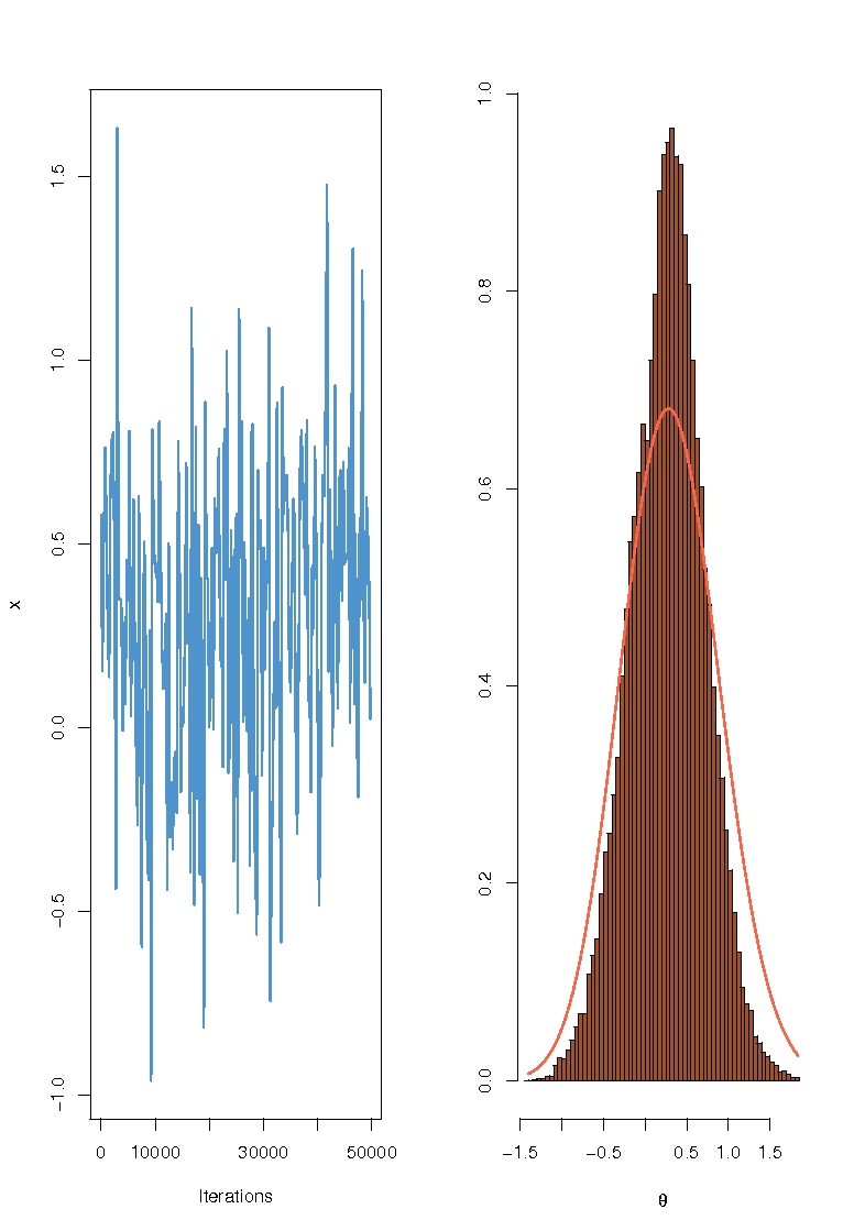
Even though the Markov chain is converging in distribution to the target distribution (when using a proper, i.e. time-homogeneous updating scheme), using past simulations to create a non-parametric approximation to the target distribution does not work either. Figure 19 shows for instance the output of an adaptive scheme in the setting of Example 18 when the proposal distribution is the Gaussian kernel based on earlier simulations. A very large number of iterations is not sufficient to reach an acceptable approximation of the target distribution.

Figure 19: Sample produced by $50,000$ iterations of a nonparametric adaptive MCMC scheme and comparison of its distribution with the target distribution.

The overall message is thus that, without further guidance, one should not constantly adapt the proposal distribution on the past performances of the simulated chain. Either the adaptation must cease after a period of burnin (not to be taken into account for the computations of expectations and quantities related to the target distribution). Else, the adaptive scheme must be theoretically assess on its own right. This later path is not easy and only a few examples can be found (so far) in the literature. See, e.g., Gilks et al. (1998) who use regeneration to create block independence and preserve Markovianity on the paths rather than on the values, Haario et al. (1999, 2001) who derive a proper adaptation scheme in the spirit of Example 18 by using a ridge-like correction to the empirical variance, and Andrieu and Robert (2001) who propose a more general framework of valid adaptivity based on stochastic optimisation and the Robbin-Monro algorithm. A more generic perspective is found in Roberts and Rosenthal (2009), who tune the random walk scale in each direction of the parameter space toward an optimal acceptance rate of $0.44$, a rate suggested in Gelman et al. (1996). Roberts and Rosenthal (2009) provide validated constraints on the tuning scheme to the extent of offering an R package called amcmc and described in Rosenthal (2007). More precisely, for each component of the simulated parameter, a factor $\delta_{i}$ corresponding to the logarithm of the random walk standard deviation is updated every $50$ iterations by adding or subtracting a factor $\epsilon_{t}$ depending on whether or not the average acceptance rate on that batch of $50$ iterations and for this component was above or below $0.44$. If $\epsilon_{t}$ decreases to zero as $\min(.01,1/\sqrt{t})$, the conditions for convergence are satisfied. (See Robert and Casella (2009, Section 8.5.2, for more details.)

0.5.2 Population Monte Carlo

To reach acceptable adaptive algorithms, while avoiding an extended study of their theoretical properties, a better alternative is to leave the setup of Markov chain simulations and to consider instead sequential or population Monte Carlo methods (Iba, 2000; Cappé et al., 2004) that have much more in common with importance sampling than with MCMC. They are inspired from particle systems that were introduced to handle rapidly changing target distributions like those found in signal processing and imaging (Gordon et al., 1993; Shephard and Pitt, 1997; Doucet et al., 2001; Del Moral et al., 2006) but primarily handle fixed but complex target distributions by building a sequence of increasingly better proposal distributions. Each iteration of the population Monte Carlo (PMC) algorithm thus produces a sample approximately simulated from the target distribution but the iterative structure allows for adaptivity toward the target distribution. Since the validation is based on importance sampling principles, dependence on the past samples can be arbitrary and the approximation to the target is valid (unbiased) at each iteration and does not require convergence times nor stopping rules.

If $t$ indexes the iteration and $i$ the sample point, consider proposal distributions $q_{it}$ that simulate the $x_{i}^{(t)}$’s and associate to each $x_{i}^{(t)}$ an importance weight

$$\varrho_{i}^{(t)}=\pi(x_{i}^{(t)})\big{/}q_{it}(x_{i}^{(t)})\,,\qquad i=1,\ldots,n\,.$$

(The proposal distribution thus depends both on the iteration and on the particle index.) Approximations of the form

$$\mathfrak{I}_{t}=\frac{1}{n}\,\sum_{i=1}^{n}\varrho_{i}^{(t)}\,h(x_{i}^{(t)})$$

are then unbiased estimators of $\mathbb{E}^{\pi}[h(X)]$, even when the importance distribution $q_{it}$ depends on the entire past of the experiment. Indeed, if $\zeta$ denotes the vector of past random variates that contribute to $q_{it}$, and $g(\zeta)$ its arbitrary distribution, we have

$$\int\int\frac{\pi(x)}{q_{it}(x|\zeta)}\,h(x)q_{it}(x)\text{d}x\,g(\zeta)\text{d}\zeta=\int\int h(x)\pi(x)\text{d}x\,g(\zeta)\text{d}\zeta=\mathbb{E}^{\pi}[h(X)]\,.$$

Furthermore, assuming that the variances

$${\mathrm{var}}\left(\varrho_{i}^{(t)}h(x_{i}^{(t)})\right)$$

exist for every $1\leq i\leq n$, we have

$${\mathrm{var}}\left(\mathfrak{I}_{t}\right)=\frac{1}{n^{2}}\ \sum_{i=1}^{n}{\mathrm{var}}\left(\varrho_{i}^{(t)}h(x_{i}^{(t)})\right)\,,$$

due to the cancelling effect of the weights $\varrho_{i}^{(t)}$.

Since, usually, the density $\pi$ is unscaled, we use instead

$$\varrho_{i}^{(t)}\propto\frac{\pi(x_{i}^{(t)})}{q_{it}(x_{i}^{(t)})}\,,\qquad i=1,\ldots,n\,,$$

scaled so that the $\varrho_{i}^{(t)}$’s sum up to $1$. In this case, the unbiasedness is lost, although it approximately holds. In fact, the estimation of the normalising constant of $\pi$ improves with each iteration $t$, since the overall average

$$\varpi_{t}=\frac{1}{tn}\,\sum_{\tau=1}^{t}\,\sum_{i=1}^{n}\,\frac{\pi(x_{i}^{(\tau)})}{q_{i\tau}(x_{i}^{(\tau)})}$$

is convergent. Therefore, as $t$ increases, $\varpi_{t}$ contributes less and less to the variability of $\mathfrak{I}_{t}$.

However, Douc et al. (2007a) have shown that this use of the importance weights $\varrho_{i}^{(t)}$ in Cappé et al. (2004) was not adaptive enough and they proposed a Rao–Blackwellised substitute

$$\varrho_{i}^{(t)}\propto\frac{\pi(x_{i}^{(t)})}{\sum_{j}q_{jt}(x_{i}^{(t)})}\,,\qquad i=1,\ldots,n\,,$$

that guaranteed an (asymptotic in $n$) improvement of the proposal at each iteration $t$, under specific forms of the $q_{it}$’s (Douc et al., 2007a, b; Cappé et al., 2008)

Since the above establishes that an simulation scheme based on sample dependent proposals is fundamentally a specific kind of importance sampling, the following algorithm is validated by the same principles as regular importance sampling:

—Population Monte Carlo Algorithm—

For $t=1,\ldots,T$ 1. For $i=1,\ldots,n$, (i) Select the generating distribution $q_{it}(\cdot)$ (ii) Generate $x_{i}^{(t)}\sim q_{it}(x)$ (iii) Compute $\varrho_{i}^{(t)}=\pi(x_{i}^{(t)})/\sum_{j}q_{jt}(x_{i}^{(t)})$ 2. Normalise the $\varrho_{i}^{(t)}$’s to sum up to $1$ 3. Resample $n$ values from the $x_{i}^{(t)}$’s with replacement, using the weights $\varrho_{i}^{(t)}$, to create the sample $(x_{1}^{(t)},\ldots,x_{n}^{(t)})$

Step (i) is singled out because it is the central property of the PMC algorithm, namely that adaptivity can be extended to the individual level and that the $q_{it}$’s can be picked based on the performances of the previous $q_{i(t-1)}$’s or even on all the previously simulated samples, if storage allows. For instance, the $q_{it}$’s can include large tails proposals as in the defensive sampling strategy of Hesterberg (1995), to ensure finite variance. Similarly, Warnes’ (2001) non-parametric Gaussian kernel approximation can be used as a proposal. (See also in Stavropoulos and Titterington, 2001 the smooth bootstrap technique as an earlier example of PMC algorithm.)

A major difference between the PMC algorithm and earlier proposals in the particle system literature is that past dependent moves as those of Gilks and Berzuini (2001) and Del Moral et al. (2006) remain within the MCMC framework, with Markov transition kernels with stationary distribution equal to $\pi$.

Example 19 (Continuation of Example 14)

We consider here the implementation of the PMC algorithm in the case of the the normal mixture (11). As in Example 15, a PMC sampler can be efficiently implemented without the (Gibbs) augmentation step, using normal random walk proposals based on the previous sample of $\boldsymbol{\mu}=(\mu_{1},\mu_{2})$’s. Moreover, the difficulty inherent to random walks, namely the selection of a “proper” scale, can be bypassed because of the adaptivity of the PMC algorithm. Indeed, the proposals can be associated with a range of variances $v_{k}$ $(1\leq k\leq K)$ ranging from, e.g., $10^{3}$ down to $10^{-3}$. At each step of the algorithm, the new variances can be selected proportionally to the performances of the scales $v_{k}$ on the previous iterations. For instance, a scale can be chosen proportionally to its non-degeneracy rate in the previous iteration, that is, the percentage of points generated with the scale $v_{k}$ that survived after resampling. The weights are then of the form

$$\varrho_{i}\propto\frac{f\left(\mathbf{x}\left|\left(\mu_{1}\right)_{i}^{(t)},\left(\mu_{2}\right)_{i}^{(t)}\right.\right)\pi\left(\left(\mu_{1}\right)_{i}^{(t)},\left(\mu_{2}\right)_{i}^{(t)}\right)}{\sum_{j=1}^{n}\varphi\left(\left(\mu_{1}\right)_{i}^{(t)}\left|\left(\mu_{1}\right)_{j}^{(t-1)},v_{k}\right.\right)\varphi\left(\left(\mu_{2}\right)_{i}^{(t)}\left|\left(\mu_{2}\right)_{j}^{(t-1)},v_{k}\right.\right)\,,}$$

where $\varphi(q|s,v)$ is the density of the normal distribution with mean $s$ and variance $v$ at the point $q$.

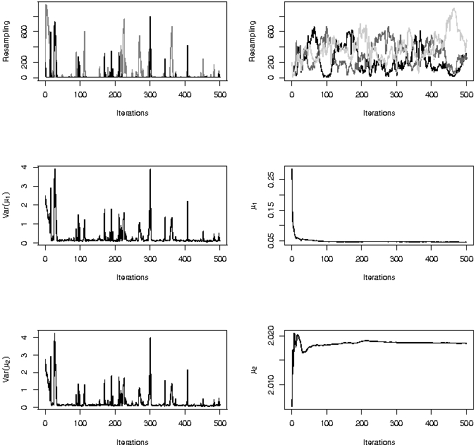
Compared with an MCMC algorithm in the same setting (see Examples 14 and 15), the main feature of this algorithm is its ability to deal with multiscale proposals in an unsupervised manner. The upper row of Figure 22 produces the frequencies of the five variances $v_{k}$ used in the proposals along iterations: The two largest variances $v_{k}$ most often have a zero survival rate, but sometimes experience bursts of survival. In fact, too large a variance mostly produces points that are irrelevant for the posterior distribution, but once in a while a point $\theta_{j}^{(t)}$ gets close to one of the modes of the posterior. When this occurs, the corresponding $\varrho_{j}$ is large and $\theta_{j}^{(t)}$ is thus heavily resampled. The upper right graph shows that the other proposals are rather evenly sampled along iterations. The influence of the variation in the proposals on the estimation of the means $\mu_{1}$ and $\mu_{2}$ can be seen on the middle and lower panels of Figure 22. First, the cumulative averages quickly stabilise over iterations, by virtue of the general importance sampling proposal. Second, the corresponding variances take longer to stabilise but this is to be expected, given the regular reappearance of subsamples with large variances.

Figure 20: Representation of the log-posterior distribution with the PMC weighted sample after $30$ iterations (the weights are proportional to the circles at each point) (Source: Cappé et al., 2004).

Figure 21: Histograms of the PMC sample: sample at iteration 5 (left) before resampling and (right) after resampling.

Figure 22: Performances of the mixture PMC algorithm for $1000$ observations from a $0.2{\cal N}(0,1)+0.8{\cal N}(2,1)$ distribution, with $\theta=1$ $\lambda=0.1$, $v_{k}=5,2,.1,.05,.01$, and a population of $1050$ particles: (upper left) Number of resampled points for the variances $v_{1}=5$ (darker) and $v_{2}=2$; (upper right) Number of resampled points for the other variances, $v_{3}=0.1$ is the darkest one; (middle left) Variance of the simulated $\mu_{1}$’s along iterations; (middle right) Cumulated average of the simulated $\mu_{1}$’s over iterations; (lower left) Variance of the simulated $\mu_{2}$’s along iterations; (lower right) Cumulated average of the simulated $\mu_{2}$’s over iterations (Source: Cappé et al., 2004).

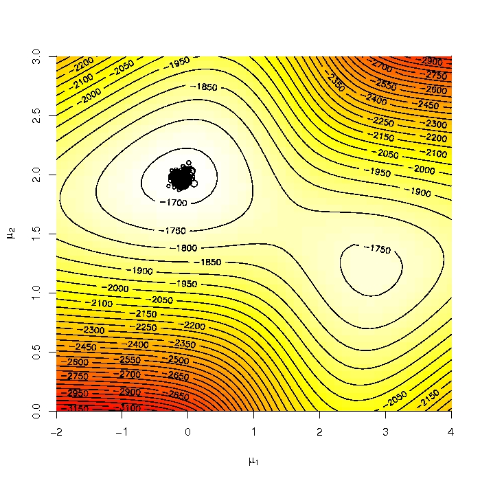
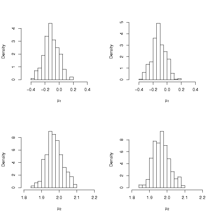
In comparison with Figures 11 and 12, Figure 20 shows that the sample produced by the PMC algorithm is quite in agreement with the modal zone of the posterior distribution. The second mode, which is much lower, is not preserved in the sample after the first iteration. Figure 21 also shows that the weights are quite similar, with no overwhelming weight in the sample.

The generality in the choice of the proposal distributions $q_{it}$ is obviously due to the abandonment of the MCMC framework. The difference with an MCMC framework is not simply a theoretical advantage: as seen in Section 0.5.1, proposals based on the whole past of the chain do not often work. Even algorithms validated by MCMC steps may have difficulties: in one example of Cappé et al. (2004), a Metropolis–Hastings scheme does not work well, while a PMC algorithm based on the same proposal produces correct answers. Population Monte Carlo algorithms offer a theoretically valid solution to the adaptivity issue, with practical gains as well, as exemplified in Wraith et al. (2009). The connection with nonparametric Bayes estimation has not yet been sufficiently pursued but the convergence of kernel-like proposals demonstrated by Cappé et al. (2008) shows this is a promising direction.

0.5.3 Approximate Bayesian computation

One particular application of the Accept–Reject algorithm that has found a niche of its own in population genetics is called approximate Bayesian computation (ABC), following the denomination proposed by Pritchard et al. (1999). It is in fact an appealing substitute for “exact” (meaning convergent) Bayesian algorithms in settings where the likelihood function $f(x|\theta)$ is not available, even up to a normalising constant, but where it can easily be simulated. The range of applications is thus much wider than population genetics and covers for instance graphical models and inverse problems.

Assuming, thus, that a posterior distribution $\pi(\theta|x_{0})\propto\pi(\theta)f(x_{0}|\theta)$ is to be simulated, a rudimentary accept-reject algorithm generates values from the prior and from the likelihood until the simulated observation is equal to the original observation $x_{0}$:
Repeat
             Generate $\theta\sim\pi(\theta)$ and $X\sim f(x|\theta)$
until $X=x_{0}$
Since the conditional probability of acceptance is $f(x_{0}|\theta)$, the distribution of the accepted $\theta$ is truly $\pi(\theta|x_{0})$, even when $f(x|\theta)$ cannot be computed.

The above algorithm is valid, but it is unfortunately restricted to settings where (a) $\pi(\theta)$ is a proper prior and (b) $\text{Pr}_{\theta}(X=x_{0})$ has a positive probability of occurrence. Even in population genetics where the outcome $X$ is a discrete random variable, the size of the state-space is often such that this algorithm cannot be implemented. The proposal of Pritchard et al. (1999) is to replace the exact acceptance condition $X=x_{0}$ in the above with an approximate condition $d(X,x_{0})<\epsilon$, where $d$ is a distance and $\epsilon$ is a tolerance level. The corresponding ABC algorithm is thus:

—Approximate Bayesian computation Algorithm—

For $i=1,\ldots,n$, 1 Generate $\theta_{i}\sim\pi(\theta)$ 2 Generate $x_{i}\sim f(x|\theta_{i})$ and compute $d(x_{0},x_{i})$ Accept the $\theta_{i}$’s such that $d(x_{i},x)<\epsilon$.

The output of the ABC algorithm is distributed from the distribution with density proportional to $\pi(\theta)\,\text{Pr}_{\theta}\{d(X,x_{0})<\epsilon\}$, where $\text{Pr}_{\theta}$ represents the sampling distribution of $X$, indexed by $\theta$. This density is somehow mistakenly denoted by $\pi\{\theta\mid d(x,x_{0})<\epsilon\}$, where the conditioning corresponds to the marginal distribution of $d(x,x_{0})$ given $x_{0}$. While unavoidable, this inherent approximation step makes the ABC method difficult to assess and to compare with regular Monte Carlo approaches, even though recent works replace it within a non-parametric framework that aims at approximating the conditional density function $f(x|\theta)$ and hence envision $\epsilon$ as a potential bandwidth (Beaumont et al., 2002; Blum and François, 2010).

Improvements on the original scheme have been achieved either by modifying the proposal distribution of the parameter $\theta$, in order to increase the density of $x$’s within the vicinity of $y$ (Marjoram et al., 2003; Bortot et al., 2007), or, as stated above, by envisioning the problem as a conditional density estimation issue and by developing techniques to allow for larger $\epsilon$ (Beaumont et al., 2002). For instance, Marjoram et al. (2003) defined a Markov chain Monte Carlo (MCMC) version of the ABC algorithm that enjoys the same validity as the original, namely that, if a Markov chain $(\theta^{(t)})$ is created via the transition function

$$\theta^{(t+1)}=\begin{cases}\theta^{\prime}\sim K(\theta^{\prime}\mid\theta^{(t)})&\text{if }x\sim f(x\mid\theta^{\prime})\text{ is such that }x=x_{0}\\ &\text{ and }u\sim\mathcal{U}(0,1)\leq\dfrac{\pi(\theta^{\prime})K(\theta^{(t)}\mid\theta^{\prime})}{\pi(\theta^{(t)})K(\theta^{\prime}\mid\theta^{(t)})}\,,\\ \theta^{(t)}&\text{otherwise,}\end{cases}$$

its stationary distribution is the posterior $\pi(\theta\mid x_{0})$. Again, in most settings, exact equality is not achievable and the above constraint $x=x_{0}$ is replaced with the approximation $d(x,x_{0})<\epsilon$. In Beaumont et al. (2009), a population Monte Carlo modification of ABC is introduced, resulting into the algorithm:

—PMC-ABC Algorithm—

Given a decreasing sequence of tolerance thresholds $\epsilon_{1}\geq\ldots\geq\epsilon_{T}$, 1. At iteration $t=1$, For $i=1,...,N$ Simulate $\theta_{i}^{(1)}\sim\pi(\theta)$ and $x\sim f(x\mid\theta_{i}^{(1)})$ until $\varrho(x,y)<\epsilon_{1}$ Set $\omega^{(1)}_{i}=1/N$ Take $\tau^{2}_{1}$ as twice the empirical variance of the $\theta_{i}^{(1)}$’s 2. At iteration $2\leq t\leq T$, For $i=1,...,N$, repeat Pick $\theta_{i}^{\star}$ from the $\theta_{j}^{(t-1)}$’s with probabilities $\omega_{j}^{(t-1)}$
generate $\theta_{i}^{(t)}\mid\theta_{i}^{\star}\sim\mathcal{N}(\theta_{i}^{\star},\tau_{t}^{2})$ and $x\sim f(x\mid\theta_{i}^{(t)})$ until $\varrho(x,y)<\epsilon_{t}$
Set $\omega^{(t)}_{i}\propto\pi(\theta^{(t)}_{i})/\sum_{j=1}^{N}\omega^{(t-1)}_{j}\varphi\left\{\tau_{t}^{-1}\left(\theta^{(t)}_{i}-\theta^{(t-1)}_{j}\right)\right\}$ Take $\tau_{t+1}^{2}$ as twice the weighted empirical variance of the $\theta_{i}^{(t)}$’s

From a practical viewpoint, the number of iterations $T$ can be controlled via the modifications in the parameters of $K_{t}$, a stopping rule being that the iterations should stop when those parameters have settled, while the more fundamental issue of selecting a sequence of $\epsilon_{t}$’s towards a proper approximation of the true posterior can rely on the stabilisation of the estimators of some quantities of interest associated with this posterior. But there is generally no fixed-cost solution that let $\epsilon_{t}$ decrease to zero with $t$. Note also that the SMC algorithm of Del Moral et al. (2006) has been recently extended to this ABC setup, making the resulting algorithm a direct competitor of the above PMC-ABC algorithm.

0.6 Conclusion

This short overview of the problems and solutions considered for Bayesian Statistics is nothing but an introduction to the game: there are much more complex problems than those illustrated above and much more advanced techniques than those presented in these pages. The reader is then encouraged to enter the literature on the topic, maybe with other introductory surveys like Cappé and Robert (2000) and Andrieu et al. (2004), but mostly through books like Chen et al. (2000), Doucet et al. (2001), Liu (2001), Robert and Casella (2004), Albert (2007), Marin and Robert (2007a), and Robert and Casella (2009).

We have not mentioned so far entries to Bayesian softwares like winBUGS, developed by the MRC Unit in Cambridge (Gilks et al., 1994; Spiegelhalter et al., 1999), Ox (Doornik et al., 2002), BATS (Pole et al., 1994), BACC (Geweke, 1999) and the Minitab package of Albert (1996), which all cover some aspects of Bayesian computing. Obviously, these packages require some expertise from the user and are thus more difficult of use than the classical open source or commercial softwares like R, Splus, Statgraphics, StatXact, SPSS or SAS. In other words, they are not black boxes that could be used by laymen with no statistical background. But this entrance fee to the use of Bayesian softwares is inevitable, given the versatile nature of Bayesian analysis: since it offers much more variability than standard inferential procedures, through the choice of prior distributions and loss functions for instance, it also requires more input from the user! And, once these preliminary steps have been overcome, the programming involved in a software like winBUGS is rather limited and certainly not harder than writing a code in R or Matlab.

As stressed in this Chapter, computational issues are central to the design and implementation of Bayesian analysis. The new era opened by the MCMC methodology has brought much more freedom in the use of Bayesian methods, as reflected by the increase of Bayesian studies in applied Statistics. As usually the case, a strong increase in the use of a methodology also sees a corresponding increase in its misuse! Inconsistent data-dependent priors and improper posteriors are sometimes appearing in studies and, more generally, the assessment of prior modelling (or even of MCMC convergence) are rarely conducted with sufficient care. This is somehow a price to pay for the wider range of Bayesian studies, while the improvement of corresponding software should bring more guidelines and warnings about these misuses of Bayesian analysis.

Acknowledgements

This work had been partly supported by the Agence Nationale de la Recherche (ANR, 212, rue de Bercy 75012 Paris) through the 2009-2012 projects Big’MC and EMILE.

Notes

1. 1 In this chapter, the denomination universal is used in the sense of uniformly over all distributions.
2. 2 To impose the stationarity constraint when the order of the $AR(p)$ model varies, it is necessary to reparameterise this model in terms of either the partial autocorrelations or of the roots of the associated lag polynomial. (See, e.g., Robert, 2007, Section 4.5.)
3. 3 In this presentation of Bayes factors, we completely bypass the methodological difficulty of defining $\pi(\theta\in\Theta_{0})$ when $\Theta_{0}$ is of measure $0$ for the original prior $\pi$ and refer the reader to Robert (2007, Section 5.2.3) and Marin and Robert (2007, Section 2.3.2) for proper coverage of this issue.
4. 4 The prior distribution can be used for importance sampling only if it is a proper prior and not a $\sigma$-finite measure.
5. 5 The constant order of the Monte Carlo error does not imply that the computational effort remains the same as the dimension increases, most obviously, but rather that the decrease (with $m$) in variation has the rate $1/\sqrt{m}$.
6. 6 The empirical (Monte Carlo) confidence interval is not to be confused with the asymptotic confidence interval derived from the normal approximation. As discussed in Robert and Casella (2004, Chapter 4), these two intervals may differ considerably in width, with the interval derived from the CLT being much more optimistic!
7. 7 An alternative to the simulation from one $\mathcal{T}(\nu,x_{i},1)$ distribution that does not require an extensive study on the most appropriate $x_{i}$ is to use a mixture of the $\mathcal{T}(\nu,x_{i},1)$ distributions. As seen in Section 0.5.2, the weights of this mixture can even be optimised automatically.
8. 8 We stress the point that this is mostly an academic exercise as, in regular settings, it is rarely the case that independent components are used for the importance function.
9. 9 Section 0.4.3 covers in greater details the setting of varying dimension problems, with the same theme that completion distributions and parameters are necessary but influential for the performances of the approximation.
10. 10 Even in the simple case of the probit model, MCMC algorithms do not always converge very quickly, as shown in Robert and Casella (2004, Chapter 14).
11. 11 It is quite interesting to see that the mixture Gibbs sampler suffers from the same pathology as the EM algorithm, although this is not surprising given that it is based on the same completion scheme.
12. 12 This wealth of possible alternatives to the completion Gibbs sampler is a mixed blessing in that their range, for instance the scale of the random walk proposals, needs to be scaled properly to avoid inefficiencies.
13. 13 The difficulty with the infinite part of the problem is easily solved in that the setting is identical to simulation problems in (countable or uncountable) infinite spaces. When running simulations in those spaces, some values are never visited by the simulated Markov chain and the chances a value is visited is related with the probability of this value under the target distribution.
14. 14 Early proposals to solve the varying dimension problem involved saturation schemes where all the parameters for all models were updated deterministically (Carlin and Chib, 1995), but they do not apply for an infinite collection of models and they need to be precisely calibrated to achieve a sufficient amount of moves between models.
15. 15 For a simple proof that the acceptance probability guarantees that the stationary distribution is $\pi(k,\theta^{(k)})$, see Robert and Casella (2004, Section 11.2.2).
16. 16 In the birth acceptance probability, the factorials $k!$ and $(k+1)!$ appear as the numbers of ways of ordering the $k$ and $k+1$ components of the mixtures. The ratio cancels with $1/(k+1)$, which is the probability of selecting a particular component for the death step.
17. 17 The “sequential” denomination in the sequential Monte Carlo methods thus refers to the algorithmic part, not to the statistical part.
18. 18 The generic Rao–Blackwellised improvement was introduced in the original MCMC paper of Gelfand and Smith (1990) and studied by Liu et al. (1994) and Casella and Robert (1996). More recent developments are proposed in Cornuet et al. (2009), in connection with adaptive algorithms like PMC.
19. 19 Using a Gaussian non-parametric kernel estimator amounts to (a) sampling from the $x_{i}^{(t)}$’s with equal weights and (b) using a normal random walk move from the selected $x_{i}^{(t)}$, with standard deviation equal to the bandwidth of the kernel.
20. 20 When the survival rate of a proposal distribution is null, in order to avoid the complete removal of a given scale $v_{k}$, the corresponding number $r_{k}$ of proposals with that scale is set to a positive value, like $1$% of the sample size.
21. 21 An R package called mcsm+ has been developed in association with Robert and Casella (2009) for training about Monte Carlo methods.

References

- Abowd et al. [1999] J. Abowd, F. Kramarz, and D. Margolis. High-wage workers and high-wage firms. Econometrica, 67:251–333, 1999.
- Albert [1996] J. Albert. Bayesian Computation Using Minitab. Wadsworth Publishing Company, 1996.
- Albert [2007] J.H. Albert. Bayesian Computation with R. Springer-Verlag, New York, 2007.
- Andrieu and Robert [2001] C. Andrieu and C.P. Robert. Controlled Markov chain Monte Carlo methods for optimal sampling. Technical Report 0125, Université Paris Dauphine, 2001.
- Andrieu et al. [2004] C. Andrieu, A. Doucet, and C.P. Robert. Computational advances for and from Bayesian analysis. Statistical Science, 19(1):118–127, 2004.
- Bauwens and Richard [1985] L. Bauwens and J.F. Richard. A 1-1 Poly- random variable generator with application to Monte Carlo integration. J. Econometrics, 29:19–46, 1985.
- Beaumont et al. [2002] M.A. Beaumont, W. Zhang, and D.J. Balding. Approximate Bayesian computation in population genetics. Genetics, 162:2025–2035, 2002.
- Beaumont et al. [2009] M.A. Beaumont, J.-M. Cornuet, J.-M. Marin, and C.P. Robert. Adaptive approximate Bayesian computation. Biometrika, 96(4):983–990, 2009.
- Berkhof et al. [2003] J. Berkhof, I. van Mechelen, and A. Gelman. A Bayesian approach to the selection and testing of mixture models. Statistica Sinica, 13:423–442, 2003.
- Blum and François [2010] M.G.B. Blum and O. François. Non-linear regression models for approximate Bayesian computation. Statistics and Computing, 20:63–73, 2010.
- Bortot et al. [2007] P. Bortot, S.G. Coles, and S.A. Sisson. Inference for stereological extremes. J. American Statist. Assoc., 102:84–92, 2007.
- Cappé and Robert [2000] O. Cappé and C.P. Robert. MCMC: Ten years and still running! J. American Statist. Assoc., 95(4):1282–1286, 2000.
- Cappé et al. [2004] O. Cappé, A. Guillin, J.-M. Marin, and C.P. Robert. Population Monte Carlo. J. Comput. Graph. Statist., 13(4):907–929, 2004.
- Cappé et al. [2005] O. Cappé, E. Moulines, and T. Rydén. Inference in Hidden Markov Models. Springer-Verlag, New York, 2005.
- Cappé et al. [2008] O. Cappé, R. Douc, A. Guillin, J.-M. Marin, and C.P. Robert. Adaptive importance sampling in general mixture classes. Statist. Comput., 18:447–459, 2008.
- Carlin and Chib [1995] B.P. Carlin and S. Chib. Bayesian model choice through Markov chain Monte Carlo. J. Royal Statist. Society Series B, 57(3):473–484, 1995.
- Casella and Robert [1996] G. Casella and C.P. Robert. Rao-Blackwellisation of sampling schemes. Biometrika, 83(1):81–94, 1996.
- Celeux et al. [2000] G. Celeux, M.A. Hurn, and C.P. Robert. Computational and inferential difficulties with mixtures posterior distribution. J. American Statist. Assoc., 95(3):957–979, 2000.
- Chen et al. [2000] M.H. Chen, Q.M. Shao, and J.G. Ibrahim. Monte Carlo Methods in Bayesian Computation. Springer-Verlag, New York, 2000.
- Chib [1995] S. Chib. Marginal likelihood from the Gibbs output. J. American Statist. Assoc., 90:1313–1321, 1995.
- Chopin [2007] N. Chopin. Inference and model choice for time-ordered hidden Markov models. J. Royal Statist. Society Series B, 69(2):269–284, 2007.
- Chopin and Robert [2010] N. Chopin and Cp.P. Robert. Properties of nested sampling. Biometrika, 2010. To appear, see arXiv:0801.3887.
- Cornuet et al. [2009] J.-M. Cornuet, J.-M. Marin, A. Mira, and C.P. Robert. Adaptive multiple importance sampling. Technical Report arXiv.org:0907.1254, CEREMADE, Université Paris Dauphine, 2009.
- Del Moral et al. [2006] P. Del Moral, A. Doucet, and A. Jasra. Sequential Monte Carlo samplers. J. Royal Statist. Society Series B, 68(3):411–436, June 2006.
- Dickey [1971] J.M. Dickey. The weighted likelihood ratio, linear hypotheses on normal location parameters. Ann. Mathemat. Statist., 42:204–223, 1971.
- Diebolt and Robert [1994] J. Diebolt and C.P. Robert. Estimation of finite mixture distributions by Bayesian sampling. J. Royal Statist. Society Series B, 56:363–375, 1994.
- Doornik et al. [2002] J.A. Doornik, D.F. Hendry, and N. Shephard. Computationally-intensive econometrics using a distributed matrix-programming language. Philo. Trans. Royal Society London, 360:1245–1266, 2002.
- Douc et al. [2007a] R. Douc, A. Guillin, J.-M. Marin, and C.P. Robert. Convergence of adaptive mixtures of importance sampling schemes. Ann. Statist., 35(1):420–448, 2007a.
- Douc et al. [2007b] R. Douc, A. Guillin, J.-M. Marin, and C.P. Robert. Minimum variance importance sampling via population Monte Carlo. ESAIM: Probability and Statistics, 11:427–447, 2007b.
- Doucet et al. [2001] A. Doucet, N. de Freitas, and N. Gordon. Sequential Monte Carlo Methods in Practice. Springer-Verlag, New York, 2001.
- Frühwirth-Schnatter [2001] S. Frühwirth-Schnatter. Markov chain Monte Carlo estimation of classical and dynamic switching and mixture models. J. American Statist. Assoc., 96(453):194–209, 2001.
- Frühwirth-Schnatter [2004] S. Frühwirth-Schnatter. Estimating marginal likelihoods for mixture and Markov switching models using bridge sampling techniques. The Econometrics Journal, 7(1):143–167, 2004.
- Frühwirth-Schnatter [2006] S. Frühwirth-Schnatter. Finite Mixture and Markov Switching Models. Springer-Verlag, New York, New York, 2006.
- Gelfand and Smith [1990] A.E. Gelfand and A.F.M. Smith. Sampling based approaches to calculating marginal densities. J. American Statist. Assoc., 85:398–409, 1990.
- Gelman et al. [1996] A. Gelman, W.R. Gilks, and G.O. Roberts. Efficient Metropolis jumping rules. In J.O. Berger, J.M. Bernardo, A.P. Dawid, D.V. Lindley, and A.F.M. Smith, editors, Bayesian Statistics 5, pages 599–608. Oxford University Press, Oxford, 1996.
- Geweke [1999] J. Geweke. Using simulation methods for Bayesian econometric models: Inference, development, and communication (with discussion and rejoinder). Econometric Reviews, 18:1–126, 1999.
- Geweke [2007] J. Geweke. Interpretation and inference in mixture models: Simple MCMC works. Comput. Statist. Data Analysis, 51(7):3529–3550, 2007.
- Gilks and Berzuini [2001] W.R. Gilks and C. Berzuini. Following a moving target–Monte Carlo inference for dynamic Bayesian models. J. Royal Statist. Society Series B, 63(1):127–146, 2001.
- Gilks et al. [1994] W.R. Gilks, A. Thomas, and D.J. Spiegelhalter. A language and program for complex Bayesian modelling. The Statistician, 43:169–178, 1994.
- Gilks et al. [1998] W.R. Gilks, G.O. Roberts, and S.K. Sahu. Adaptive Markov chain Monte Carlo. J. American Statist. Assoc., 93:1045–1054, 1998.
- Gordon et al. [1993] N. Gordon, J. Salmond, and A.F.M. Smith. A novel approach to non-linear/non-Gaussian Bayesian state estimation. IEEE Proceedings on Radar and Signal Processing, 140:107–113, 1993.
- Green [1995] P.J. Green. Reversible jump MCMC computation and Bayesian model determination. Biometrika, 82(4):711–732, 1995.
- Haario et al. [1999] H. Haario, E. Saksman, and J. Tamminen. Adaptive proposal distribution for random walk Metropolis algorithm. Computational Statistics, 14(3):375–395, 1999.
- Haario et al. [2001] H. Haario, E. Saksman, and J. Tamminen. An adaptive Metropolis algorithm. Bernoulli, 7(2):223–242, 2001.
- Hesterberg [1995] T. Hesterberg. Weighted average importance sampling and defensive mixture distributions. Technometrics, 37:185–194, 1995.
- Iba [2000] Y. Iba. Population-based Monte Carlo algorithms. Trans. Japanese Soc. Artificial Intell., 16(2):279–286, 2000.
- Jasra et al. [2005] A. Jasra, C.C. Holmes, and D.A. Stephens. Markov Chain Monte Carlo methods and the label switching problem in Bayesian mixture modeling. Statist. Sci., 20(1):50–67, 2005.
- Jeffreys [1961] H. Jeffreys. Theory of Probability. Oxford Classic Texts in the Physical Sciences. Oxford University Press, Oxford, third edition, 1961.
- Lee et al. [2009] K. Lee, J.-M. Marin, K.L. Mengersen, and C.P. Robert. Bayesian inference on mixtures of distributions. In N.S. Narasimha Sastry, M. Delampady, and B. Rajeev, editors, Perspectives in Mathematical Sciences I: Probability and Statistics, pages 165–202. World Scientific, Singapore, 2009.
- Liu [2001] J.S. Liu. Monte Carlo Strategies in Scientific Computing. Springer-Verlag, New York, 2001.
- Liu et al. [1994] J.S. Liu, W.H. Wong, and A. Kong. Covariance structure of the Gibbs sampler with applications to the comparisons of estimators and sampling schemes. Biometrika, 81:27–40, 1994.
- Marin and Robert [2007a] J.-M. Marin and C.P. Robert. Bayesian Core. Springer-Verlag, New York, 2007a.
- Marin and Robert [2007b] J.-M. Marin and C.P. Robert. Importance sampling methods for Bayesian discrimination between embedded models. In M.-H. Chen, D.K. Dey, P. Müller, D. Sun, and K. Ye, editors, Frontiers of Statistical Decision Making and Bayesian Analysis. Springer-Verlag, New York, 2007b. To appear, see arXiv:0910.2325.
- Marjoram et al. [2003] P. Marjoram, J. Molitor, V. Plagnol, and S. Tavaré. Markov chain Monte Carlo without likelihoods. Proc. Natl. Acad. Sci. USA, 100(26):15324–15328, December 2003.
- McCullagh and Nelder [1989] P. McCullagh and J. Nelder. Generalized Linear Models. Chapman and Hall, New York, 1989.
- Meng and Wong [1996] X.L. Meng and W.H. Wong. Simulating ratios of normalizing constants via a simple identity: a theoretical exploration. Statist. Sinica, 6:831–860, 1996.
- Metropolis and Ulam [1949] N. Metropolis and S. Ulam. The Monte Carlo method. J. American Statist. Assoc., 44:335–341, 1949.
- Neal [2003] R.M. Neal. Slice sampling (with discussion). Ann. Statist., 31:705–767, 2003.
- Nobile [1998] A. Nobile. A hybrid Markov chain for the Bayesian analysis of the multinomial probit model. Statistics and Computing, 8:229–242, 1998.
- Pole et al. [1994] A. Pole, M. West, and P.J. Harrison. Applied Bayesian Forecasting and Time Series Analysis. Chapman-Hall, New York, 1994.
- Pritchard et al. [1999] J.K. Pritchard, M.T. Seielstad, A. Perez-Lezaun, and M.W. Feldman. Population growth of human Y chromosomes: a study of Y chromosome microsatellites. Mol. Biol. Evol., 16:1791–1798, 1999.
- Richardson and Green [1997] S. Richardson and P.J. Green. On Bayesian analysis of mixtures with an unknown number of components (with discussion). J. Royal Statist. Society Series B, 59:731–792, 1997.
- Robert [2007] C.P. Robert. The Bayesian Choice. Springer-Verlag, New York, paperback edition, 2007.
- Robert and Casella [2004] C.P. Robert and G. Casella. Monte Carlo Statistical Methods. Springer-Verlag, New York, second edition, 2004.
- Robert and Casella [2009] C.P. Robert and G. Casella. Introducing Monte Carlo Methods with R. Springer-Verlag, New York, 2009.
- Robert and Casella [2010] C.P. Robert and G. Casella. A history of Markov chain Monte Carlo-subjective recollections from incomplete data. In S. Brooks, A. Gelman, X.L. Meng, and G. Jones, editors, Handbook of Markov Chain Monte Carlo: Methods and Applications. Chapman and Hall, New York, 2010. arXiv0808.2902.
- Robert and Marin [2009] C.P. Robert and J.-M. Marin. On resolving the Savage–Dickey paradox. Technical Report arxiv.org:0910.1452, CEREMADE, Université Paris Dauphine, 2009.
- Robert and Wraith [2009] C.P. Robert and D. Wraith. Computational methods for Bayesian model choice. In Paul M. Goggans and Chun-Yong Chan, editors, MaxEnt 2009 proceedings, volume 1193. AIP, 2009.
- Roberts and Rosenthal [2009] G.O. Roberts and J.S. Rosenthal. Examples of adaptive MCMC. J. Comp. Graph. Stat., 18:349–367, 2009.
- Roeder [1992] K. Roeder. Density estimation with confidence sets exemplified by superclusters and voids in galaxies. J. American Statist. Assoc., 85:617–624, 1992.
- Rosenthal [2007] J.S. Rosenthal. Amcm: An R interface for adaptive MCMC. Comput. Statist. Data Analysis, 51:5467–5470, 2007.
- Shephard and Pitt [1997] N. Shephard and M.K. Pitt. Likelihood analysis of non-Gaussian measurement time series. Biometrika, 84:653–668, 1997.
- Skilling [2006] J. Skilling. Nested sampling for general Bayesian computation. Bayesian Analysis, 1(4):833–860, 2006.
- Spiegelhalter et al. [1999] D.J. Spiegelhalter, A. Thomas, and N.G. Best. WinBUGS Version 1.2 User Manual. Cambridge, 1999.
- Stavropoulos and Titterington [2001] P. Stavropoulos and D.M. Titterington. Improved particle filters and smoothing. In A. Doucet, N. deFreitas, and N. Gordon, editors, Sequential MCMC in Practice. Springer-Verlag, New York, 2001.
- Tanner and Wong [1987] M. Tanner and W. Wong. The calculation of posterior distributions by data augmentation. J. American Statist. Assoc., 82:528–550, 1987.
- Verdinelli and Wasserman [1995] I. Verdinelli and L. Wasserman. Computing Bayes factors using a generalization of the Savage–Dickey density ratio. J. American Statist. Assoc., 90:614–618, 1995.
- Wraith et al. [2009] D. Wraith, M. Kilbinger, K. Benabed, O. Cappé, J.-F. Cardoso, G. Fort, S. Prunet, and C.P. Robert. Estimation of cosmological parameters using adaptive importance sampling. Physical Review D, 80:023507, 2009.
Index
- ABC §0.5.3
-
acceptance probability
- reverse move §0.4.3
- acceptance rate
adaptivity §0.5.1, §0.5.1, §0.5.2
- invalid 18
- algorithm
amcmc+ §0.5.1 - approximate Bayesian computation (ABC) §0.5.3
AR model 17, 3, 7
- order 3
autocorrelation
- partial endnote 2
Bayes
- theorem §0.2.3
- Bayes factor §0.2.2
- Bayesian
- Bertillon, Alphonse 14
- birth-and-death process 16
bootstrap
- smooth §0.5.2
- bridge
- Central Limit Theorem §0.3.1
- Chib’s approximation §0.3.3
- completion 14
- computational effort §0.3.1
- confidence
- convergence assessment §0.3.1
- curse of dimension §0.3.2, item (a)
dataset
- employment 2
- large item (iii)
- Pima Indian diabetes Figure 7
- Decision theory §0.2.1
- defensive sampling §0.5.2
- dimension
- distribution
- estimation vs. testing §0.2.3
- estimator
- evidence §0.3.3
- exponential family 2
fit
- data 3
- function
Gibbs sampler §0.4.2—§0.4.2
- mixing of 14
- harmonic mean §0.3.3
- heterogeneous populations §0.2.3, 14
- highest posterior region §0.2.2
- hypotheses §0.2.1
- identifiability §0.2.1
- importance function §0.3.1
- importance sampling
- infinite collection of models item –
- integral
- label switching problem 14
- Law of Large Numbers §0.3.1
likelihood
- intractable item (iii), §0.5.3
- marginal §0.3.3
- ratio §0.2.2
- Markov chain Monte Carlo (MCMC) algorithm §0.4—§0.4.3
mcsm+ §0.6 - military conscripts 14
missing variables
- simulation of §0.4.2
- mixture
mixtures
- and latent variables 14
- mode
- model
- model averaging §0.2.3
- model choice §0.2.3
- Monte Carlo techniques §0.3—§0.3.3
- Neyman–Pearson theory §0.2.2
- normal approximation endnote 6
normalising constant §0.3.1, §0.3.3
- ratios of §0.3.3
parameter item (i)
- of interest §0.2.1
parameter space item (i), 2nd item, §0.2.3
- constrained item (i)
- particle systems §0.5.2
- PMC vs. MCMC 19
- poly- distribution 1
- population Monte Carlo (PMC) techniques endnote 17
- posterior distribution 2
prediction §0.2.1
- sequential item (iii)
- prior distribution item (ii)
- proposal
- -value §0.2.2
- R §0.6
- Rao–Blackwellisation §0.5.2
- ratio
- reversible jump MCMC §0.4.3, §0.4.3—§0.4.3
- sampling
- scaling
- simulation §0.3, §0.3.1
- smooth bootstrap §0.5.2
- space
- stationarity endnote 2
- Statistics
- stopping rule §0.5.2
survival rate
- null 19
- variance endnote 20
-distribution §0.2.1
- folded 9
- tempering §0.4.2
- testing hypotheses §0.2.1
- trapping state 14