Upper and lower Higgs boson mass bounds from a chirally invariant lattice Higgs-Yukawa model
DISSERTATION
zur Erlangung des akademischen Grades
doctor rerum naturalium
(Dr. rer. nat.)
im Fach Physik
eingereicht an der
Mathematisch-Naturwissenschaftlichen
Fakultät I
Humboldt-Universität zu Berlin
Prof. Dr. Dr. h.c. Christoph Markschies
Dekan der Mathematisch-Naturwissenschaftlichen
Fakultät I:
Prof. Dr. Lutz-Helmut Schön
Gutachter: 1. Prof. Dr. Michael Müller-Preussker 2. Dr. habil. Karl Jansen 3. Prof. Dr. Andreas Wipf eingereicht am: 23. Juli 2009 Tag der mündlichen Prüfung: 15. Oktober 2009
)
Abstract
Motivated by the advent of the Large Hadron Collider (LHC) the aim of the present work is the non-perturbative determination of the cutoff-dependent upper and lower mass bounds of the Standard Model Higgs boson based on first principle calculations, in particular not relying on additional information such as the triviality property of the Higgs-Yukawa sector or indirect arguments like vacuum stability considerations. For that purpose the lattice approach is employed to allow for a non-perturbative investigation of a chirally invariant lattice Higgs-Yukawa model, serving here as a reasonable simplification of the full Standard Model, containing only those fields and interactions which are most essential for the intended Higgs boson mass determination. These are the complex Higgs doublet as well as the top and bottom quark fields and their mutual interactions. To maintain the chiral character of the Standard Model Higgs-fermion coupling also on the lattice, the latter model is constructed on the basis of the Neuberger overlap operator, obeying then an exact global lattice chiral symmetry.
Respecting the fermionic degrees of freedom in a fully dynamical manner by virtue of a PHMC algorithm appropriately adapted to the here intended lattice calculations, such mass bounds can indeed be established with the aforementioned approach. Supported by analytical calculations performed in the framework of the constraint effective potential, the lower bound is found to be approximately at a cutoff of . The emergence of a lower Higgs boson mass bound is thus a manifest property of the pure Higgs-Yukawa sector that evolves directly from the Higgs-fermion interaction for a given set of Yukawa coupling constants. Its quantitative size, however, turns out to be non-universal in the sense, that it depends on the specific form, for instance, of the Higgs boson self-interaction.
The upper Higgs boson mass bound is then established in the strong coupling regime of the considered Higgs-Yukawa model. After the infinite volume extrapolation it is found to be approximately at a cutoff of . The cutoff-dependence of this upper bound can also be resolved and it is found to be in agreement with the expected logarithmic decline with increasing cutoff according to the triviality picture of the Higgs-Yukawa sector. Moreover, a direct comparison of the latter cutoff-dependent mass bound with corresponding results obtained in the pure -theory, neglecting all fermion contributions, is considered with the intention to identify the fermion contribution to the upper mass bound. However, higher statistics is required to draw a clear conclusion in this matter.
Finally, a first account on the applicability of Lüscher’s method for the determination of the Higgs boson decay width in the framework of the here considered Higgs-Yukawa model is presented. At small renormalized quartic coupling constant the obtained decay width is in good agreement with corresponding perturbative results, the validity of which is trustworthy according to being small. The good agreement thus encourages to further pursue this approach in some follow-up investigations to eventually establish an upper bound also for the decay width of the Standard Model Higgs boson.
Zusammenfassung
Motiviert durch die Inbetriebnahme des Large Hadron Colliders (LHC) liegt die Zielsetzung der vorliegenden Arbeit in der nicht-perturbativen Bestimmung der Cutoff abhängigen oberen und unteren Massenschranken des Higgs-Teilchens im Standardmodell auf der Basis von Rechnungen, die nur auf grundlegenden Prinzipien beruhen und sich insbesondere nicht auf zusätzliche Informationen stützen, wie zum Beispiel die Trivialitätseigenschaften des Higgs-Yukawa Sektors oder etwa Stabilitätsbetrachtungen des Vakuumszustandes. In dieser Arbeit wird der Gitteransatz verwendet, um eine nicht-perturbative Untersuchung eines chiral invarianten Higgs-Yukawa Modells zu ermöglichen, welches hier als eine sinnvolle Vereinfachung des vollen Standardmodells dient, und daher nur diejenigen Felder und Wechselwirkungen beinhaltet, die die Generierung der größten Beiträge zu den gesuchten Massenschranken erwarten lassen. Dies sind hier das komplexwertige Higgs-Dublett sowie die Top- und Bottom-Quarkfelder und ihre gegenseitigen Wechselwirkungen. Um die chiralen Eigenschaften der Higgs-Fermion Kopplung des Standardmodells auch auf dem Gitter zu bewahren, ist das betrachtete Higgs-Yukawa Modell auf der Grundlage des Neuberger Dirac Operators konstruiert, so dass es eine globale chirale Symmetrie, bzw. deren Gitterpendant, besitzt.
In der vorliegenden Arbeit werden die fermionischen Freiheitsgrade vollständig dynamisch berücksichtigt. Dies wird durch die Verwendung eines für das Higgs-Yukawa Modell entsprechend angepassten PHMC Algorithmus ermöglicht. Die vorgenannten Massenschranken können dann durch eine numerische Auswertung des betrachteten Modells bestimmt werden. Unterstützt durch analytische Rechnungen auf der Grundlage des effektiven Potentials findet man eine untere Schranke von näherungsweise bei einem Cutoff von . Das Auftreten einer unteren Massenschranke des Higgs Bosons ist also eine grundlegende Eigenschaft des reinen Higgs-Yukawa Sektors, welche für einen gegebenen Satz von Yukawa Kopplungskonstanten unmittelbar durch die Higgs-Fermion Wechselwirkung generiert wird. Es stellt sich jedoch heraus, dass die beobachtete quantitative Größe dieser Schranke in dem Sinne nicht universell ist, als sie von der speziellen Form der zugrunde liegenden Wechselwirkungen, zum Beispiel von der gewählten Form der bosonischen Selbstwechselwirkung, abhängt.
Die obere Schranke wird dann durch die Untersuchung des Modells im starken Kopplungsbereich bestimmt. Nach der Extrapolation in das unendliche Volumen findet man als obere Schranke näherungsweise bei einem Cutoff von . Die Cutoff-Abhängigkeit der vorgenannten oberen Schranke kann ebenfalls aufgelöst werden. Entsprechend dem Trivialitätsbild zeigt sich diese in voller Übereinstimmung mit dem erwarteten logarithmischen Abfall bei steigenden Werten des Cutoff Parameters. Darüber hinaus werden die hier bestimmten Massenschranken auch mit entsprechenden Resultaten aus der reinen -Theorie verglichen mit der Zielsetzung, den fermionischen Beitrag zur oberen Massenschranke zu identifizieren. Es ist jedoch eine höhere Statistik notwendig, um ein zuverlässiges Ergebnis in dieser Fragestellung zu erhalten.
Schließlich wird außerdem ein erster Ausblick auf die Anwendbarkeit von Lüscher’s Methode zur Bestimmung der Higgs Boson Zerfallsbreite im hier betrachteten Higgs-Yukawa Modell gegeben. Es zeigt sich, dass die vorgenannte Zerfallsbreite bei kleinen Werten der quartischen Kopplungskonstante in guter Übereinstimmung mit entsprechenden perturbativen Ergebnissen steht, welche aufgrund der klein gewählten Werte für vertrauenswürdig sind. Diese gute Übereinstimmung motiviert, den betrachteten Ansatz in zukünftigen Studien zu verwenden, um dann auch obere Grenzen für die Zerfallsbreite des Higgs Bosons bestimmen zu können.
To Cornelia,
my love.
Chapter 1 Introduction
With their postulation of the quark model, categorizing all so far discovered hadronic matter as bound states of the so-called up-, down-, and strange-quarks, Gell-Mann and Zweig laid one of the corner stones for our current understanding of Nature’s most fundamental processes [1, 2]. Equally driven by theoretical considerations as well as accelerator experiments with ever increasing accessible energy scales and precision this initial picture of the quark model was gradually extended over the subsequent decades. In today’s perspective on elementary particle physics all matter is assumed to be composed of leptons and quarks coming in three generations, each of which consisting of an up-type and a down-type quark as well as an electron-type and a neutrino-type lepton [3], as listed in Tab. 1.1. These elementary constituents mutually interact through four fundamental forces, which are the gravitation, the strong interaction, the electromagnetic force, and the weak interaction.
While most macroscopic physical processes in our universe are dominated by gravitation, which can be well described by Einstein’s classical General Relativity Theory [4] at sufficiently large distances, this situation changes completely at the microscopic scale of elementary processes. In that regime gravitation is supposed to be negligible as compared to the other three fundamental forces, unless the energy scale of the considered process becomes of the order of the Planck scale . It is only this latter situation where an otherwise hidden, potential quantum structure of gravitation is assumed to become visible and to dominate physical processes again. Despite a strenuously pursued and ongoing search for a consistent quantum theory of gravitation based, for instance, on the competing approaches of String Theory [5] and Loop-Quantum Gravity [6], such a theory could not be established yet. The resulting inherent necessity of neglecting gravity in any present theory of elementary particles, however, is generally considered as acceptable at energy scales far below the Planck scale for the aforementioned reasons.
Contrary to the current situation with respect to understanding the intrinsic quantum nature of gravitation, consistent quantum field theoretical formulations of the other three fundamental forces have successfully been devised on the basis of a common concept, which is the principle of local gauge invariance [7]. This idea initially emerged during the development of a quantum theory of electromagnetism and finally led to the evolution of quantum electrodynamics (QED), the foundation of which being a local gauge symmetry based on the gauge group with the latter subscript indicating the electric charge to be its generating operator [8]. In this framework the electromagnetic force, interacting between all particles carrying an electric charge, is modeled through the exchange of a single type of gauge boson, which is the photon in the case of QED. Strong evidence for the aforementioned gauge principle to be indeed a fundamental concept of Nature’s most elementary processes is manifest in the impressively accurate agreement between the theoretical predictions arising from QED and corresponding experimental measurements, culminating in the coincidence of the perturbatively calculated anomalous magnetic moment of the electron with its phenomenological value up to a precision of at least nine significant digits [9, 10].
| 1. Generation | 2. Generation | 3. Generation | |
|---|---|---|---|
| Leptons | |||
| Quarks |
Driven by the great success of QED, the concept of local gauge invariance has also been applied to the description of the strong interactions, which finally led to the development of quantum chromodynamics (QCD) based on the gauge group with the latter subscript indicating the respective group elements to act on the so-called colour index assigned to all quark fields [11]. The introduction of the colour index has previously been found to be inevitable to overcome Pauli’s exclusion principle, which otherwise would contradict the observation, for instance, of the -baryon consisting of three identical quarks with equal spin orientations [12]. As listed in Tab. 1.1 the leptonic fields, on the other hand, do not carry this additional index in agreement with their non-participation in the strong interaction. In the framework of QCD these forces among the quarks are considered to be mediated by the exchange of so-called gluons, being the gauge bosons of the colour group. The probably most striking feature of QCD is its ability to explain the asymptotic freedom [13, 14] of quarks at small spatial separations, manifest through the phenomenological observation of Bjorken scaling [15] in deep inelastic scattering experiments [16], while accounting also for the phenomenological non-observation of free quarks according to the concept of quark confinement [17]. Though not rigorously proven yet, the latter picture of quark confinement can presumably be explained in the framework of QCD by the emergence of a separation independent force acting between remote quarks at large spatial separations. To overcome the aforementioned uncertainty ongoing effort is currently invested in the elaborate investigation of the confinement picture, see e.g. LABEL:book:Greensite and the references therein.
In contrast to the electromagnetic and the strong forces, the weak interaction, the effects of which were first observed in the -decay of nuclei, acts differently on left- and right-handed particles. The latter left-right asymmetry becomes most apparently reflected by our current understanding that right-handed neutrinos do not interact with any of the fundamental forces, or equivalently, that right handed-neutrinos do not exist at all as indicated in Tab. 1.1.
A reasonably good understanding of the weak interaction at low energies could be provided by the (V-A)-Fermi theory [19, 20], accounting for the chiral nature of that interaction by introducing different coupling structures for the vector and axial-vector currents. This approach, however, turned out to be non-renormalizable due to a fermionic four-point coupling term explicitly appearing in the underlying Lagrangian, thus rendering the (V-A)-Fermi theory to be at most an effective model that cannot be assumed to remain valid in the limit of large energy scales. Instead, it eventually has to to go over into some more complete, renormalizable theory, a candidate for which has later been devised by Glashow, Salam, and Weinberg [21, 22, 23]. The key idea finally leading to the renormalizability [24, 25, 26] of this so-called GSW-theory is to apply the concept of local gauge invariance also to the weak interaction by modeling the latter forces as being mediated through the exchange of gauge bosons.
The gauge group underlying the GSW-theory is the direct product , where the subscripts indicate that the symmetry only refers to the left-handed doublets listed in Tab. 1.1, and that the underlying generating operator of the gauge group is actually given by the so-called hypercharge , which differs for left- and right-handed particles in agreement with the chiral character of the weak interaction. With an adequate reparametrization the four gauge bosons of the aforementioned gauge group can then be identified as the three bosons , associated to the weak interaction as well as the photon mediating the electromagnetic force, thus yielding an unified description of the so-called electroweak interaction incorporating both of the two latter forces. It is this observation which finally allowed to establish an unified formulation of the strong, the weak, and the electromagnetic interactions based on a common principle, which is the concept of local gauge invariance with respect to the group
| (1.1) |
This local gauge symmetry constitutes the foundation of the so-called Standard Model of elementary particles [27], being one of the most thoroughly and successfully tested models [28] that have so far been conceived in elementary particle physics.
The outstanding success of the underlying GSW-theory became first heralded through the theoretical prediction [23] of the only later experimentally confirmed [29, 30, 31] masses of the and bosons, which have to be massive to explain the typically very short interaction range of the weak forces. Remarkably, the aforementioned mass generation of the and gauge bosons is describable in the framework of the GSW-theory without the inclusion of any explicit mass terms into the underlying Lagrangian, which otherwise would have destroyed the renormalizability of that theory. Instead a gauge invariant and renormalizable [24, 25, 26] mechanism of mass generation could be established within the GSW-theory, known as the celebrated Higgs-mechanism [32, 33, 34], which explains the emergence of all fundamental particle masses and those of the massive and gauge bosons, as the consequence of spontaneous symmetry breaking [35, 36, 37]. This mechanism is based on the postulated existence of an additional scalar field , interacting with the fermions by means of the so-called Yukawa couplings [38], the strength of which is controlled by the respective Yukawa coupling constants, and interacting also with the latter gauge bosons and through the appearance of its covariant derivative in the underlying Lagrangian. The aforementioned concept of spontaneous symmetry breaking then refers to Nature’s selection of a particular ground state out of a manifold of degenerate vacua, such that expectation values with respect to the particular vacuum can break the intrinsic symmetries of the underlying Lagrangian. In the framework of the Standard Model the original gauge symmetry based on the gauge group in Eq. (1.1) is spontaneously broken according to
| (1.2) |
thus maintaining only the colour and the electromagnetic local gauge symmetry. The consequences of this spontaneous symmetry breaking are then most apparently reflected by the vacuum expectation value of the introduced scalar field acquiring a non-zero value , which will be labeled as ’vev’ in the following.
In the broken phase the boson masses and as well as the fermion masses are then generated through the implicit generation of corresponding mass terms in the Lagrangian arising from the aforementioned coupling structures, while the underlying theory still remains renormalizable [25]. The scalar field itself, which is actually defined as a complex doublet valued field, can then be decomposed by virtue of the Goldstone theorem [37, 39] into a massive mode , the so-called Higgs mode, as well as three massless modes , , denoted as Goldstone modes. The latter Goldstone modes, however, do not refer to additional, physically observable particles themselves but instead become identified as the longitudinal polarization modes of the three – now massive – gauge bosons and , which is often expressed by the sloppy formulation that ’the Goldstone modes are eaten by the massive gauge bosons’.
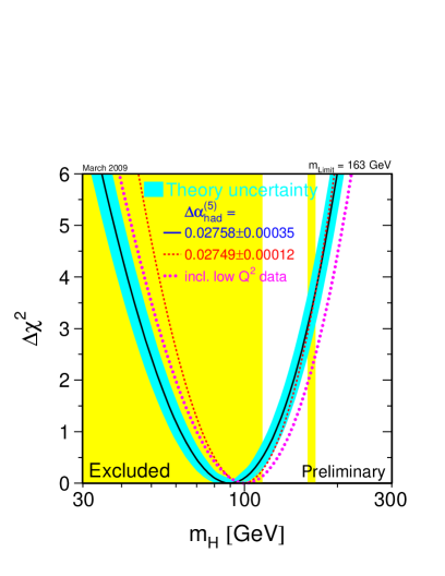
Associated to the emerging massive Higgs mode is a corresponding massive physical particle denoted as the Higgs boson that should in principle be observable in accelerator experiments. Though not discovered yet, its existence is widely considered as very likely according to the aforementioned great success of the Standard Model in general and the GSW-theory in particular. The ongoing search for the Higgs boson, being one of the main driving forces behind the construction of the Large Hadron Collider (LHC) [40], has so far excluded the existence of a Higgs particle with a mass below at the confidence level [10, 41] leaving open, however, the possibility of an even heavier Higgs boson. Apart from these exclusion limits arising from direct Higgs searches, one can also derive information on the probability distribution of the expected value for the Higgs boson mass by comparing high precision electroweak measurements with corresponding theoretical predictions arising from the Standard Model under the assumption of a particular Higgs boson mass. The aforementioned direct exclusion limit and an example of the latter probability distribution are presented together in Fig. 1.1a which has been taken from LABEL:LEPEWWGHomePage. From these data one can infer that a rather light Higgs boson mass between and is to be expected.
In contrast to the situation of the gauge bosons and , the masses of which could successfully be predicted by virtue of the GSW-theory on the basis of some at that time available low energy quantities, the Higgs boson mass itself cannot directly be estimated from that theory due to its immediate dependence on the unknown strength of the Higgs self-interaction. In the Standard Model the latter self-interaction is assumed to be of the form with the bare quartic coupling constant being apriori unconstrained. At tree-level one finds the Higgs boson mass to be given through , where the renormalized vacuum expectation value is phenomenologically known. The renormalized quartic self-coupling constant , however, is so far undetermined and could in principle take any value due to the unconstrained interval of eligible bare coupling constants , leaving thus apriori open the possibility of an arbitrarily large Higgs boson mass.
A careful analysis of the pure Higgs sector of the Standard Model, however, reveals the underlying Higgs self-coupling structure to be trivial [42, 43, 44, 45, 46, 47, 48] in four space-time dimensions. The notion of triviality refers here to the behaviour of the renormalized quartic coupling constant in dependence on the cutoff parameter . The latter cutoff has to be introduced to regularize the considered theory, yielding only then a mathematically well defined model with all otherwise divergent loop integrals, appearing for instance in the perturbative evaluation of the theory, rendered finite. In a renormalizable theory this auxiliary parameter can later be removed again in the sense of sending it to infinity while holding all physical observables constant, making the physical predictions arising from such a theory eventually independent from the previously introduced auxiliary parameter , as desired. This is generally referred to as the renormalization procedure. In a trivial theory, however, all renormalized coupling constants vanish as functions of in the limit , leading thus to a free, non-interacting theory when trying to remove the cutoff parameter by sending it to infinity.
At least two consequences arise from the latter observation. The first is that the Higgs sector of the Standard Model can only be considered as an effective theory inherently connected with a non-removable cutoff parameter , which can be interpreted as the maximal energy scale up to which the underlying effective theory can be valid at most. The description of physical processes with even larger energy scales would thus require an extension of the considered theory beyond the latter scale . As a second consequence the renormalized quartic coupling constant at a given cutoff parameter is bounded from above according to directly translating also into corresponding upper bounds on the Higgs boson mass itself.
The remarkable conclusion that can be drawn when combining the latter two observations is the following: Once the Higgs boson has actually been discovered, for instance at the LHC, and its physical mass is eventually known, it would be possible to infer from the comparison of with its cutoff-dependent upper bound up to which energy scale the Standard Model can be valid at most. Such a consideration is of fundamental interest, since it provides essential information concerning the development of future extensions to the Standard Model which, despite its tremendous success, leaves a couple of urging questions unanswered. Among them are, for instance, the so far lacking explanation for dark matter and dark energy [49], the observed neutrino oscillations [50], the baryon asymmetry [51], and the hierarchy problem [52]. It is moreover unclear, how gravitation can be incorporated into the Standard Model, whether there are more than the so far observed three quark and lepton generations, and whether the rather large number of parameters in the Standard Model can be reduced by some further unification of the strong and the electroweak interactions. Promising candidates for solving at least some of the aforementioned problems in part are, for instance, the Minimal Supersymmetric Standard Model [53], String Theory [5], Loop Quantum Gravity [6], Grand Unified Theories [54], Little Higgs Models [55], and Extra Dimensions [56]. Having the phenomenological value of the Higgs boson mass at hand would then allow to specify an energy scale from which on an extension of the Standard Model, potentially according to one of the aforementioned approaches, becomes definitely necessary.
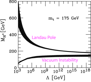
This latter energy scale can further be narrowed, since a cutoff-dependent lower Higgs boson mass bound can also be established, however not on the basis of the triviality property of the considered model. In renormalized perturbation theory such cutoff-dependent lower bounds have been derived from vacuum stability considerations, see e.g. LABEL:Cabibbo:1979ay,_Linde:1975sw,Weinberg:1976pe,Linde:1977mm,_Sher:1988mj,_Lindner:1988ww,_Altarelli:1994rb,Casas:1994qy,_Casas:1996aq, while corresponding upper bounds have been established based on the criterion of the Landau pole being situated beyond the cutoff of the theory, see e.g. LABEL:Cabibbo:1979ay,_Dashen:1983ts,_Lindner:1985uk, as well as from unitarity requirements, see e.g. LABEL:Dicus:1992vj,_Lee:1977eg,_Marciano:1989ns. A review on these various calculations of the sought-after cutoff-dependent upper and lower Higgs boson mass bounds can be found in LABEL:Hagiwara:2002fs, the summarizing plot of which is presented in Fig. 1.1b. From these already established results one can, for instance, infer that an extension of the Standard Model would become inevitable at energy scales beyond , in case the Higgs boson mass would be found to be lighter than .
 |
 |
| (a) | (b) |
However, the results relying on the aforementioned vacuum instability arguments have to be considered with care. In the underlying calculations the effective potential has been determined in terms of the renormalized coupling constants by means of perturbation theory. It is then usually found that the renormalized expression for the effective potential exhibits an instability, meaning that the effective potential becomes unbounded from below, if the Higgs boson mass becomes too small for a given setting of the renormalized fermion masses, thus inducing a lower bound on the Higgs boson mass, as desired. It is, however, also known that the effective potential is convex for all values of the bare coupling constants, where the underlying theory is well-defined, and can therefore never be unstable [72], which is apparently in contrast to the aforementioned observation of an unstable effective potential at small values of the Higgs boson mass. Additionally, it has recently been argued that the appearance of a vacuum instability in the renormalized calculation is actually caused by the incorrect removal of the cutoff from the underlying trivial theory [73, 74].
This apparent paradox can be resolved [75], if one keeps in mind that the definition domain of any renormalized quantity might be constrained, though its bare counterpart is not. This is particularly obvious in the framework of a trivial theory, such as the Higgs-Yukawa sector of the Standard Model. In that scenario the bare quartic coupling constant can take any positive value, but its renormalized counterpart is constrained to , where the latter bounds are apriori undetermined. For clarification it is pointed out again that the cutoff always has to be kept finite due to the triviality of the model, since otherwise one would inevitably end up with being the only eligible choice for the renormalized quartic coupling constant. As long as one chooses the renormalized coupling constants underlying the perturbative calculation of the effective potential according to their respective definition domains, the arising result on the latter potential will actually refer to a certain configuration of bare model parameters at the considered cutoff, for which the effective potential is known to be convex. If, however, one chooses the aforementioned renormalized coupling constants not to be contained within their respective definition domains, then one cannot establish a connection of the arising renormalized result on the effective potential, which might predict an instability, to any configuration of bare parameters. In case of this can be expressed by saying that the associated bare quartic coupling constant is negative. For one therefore actually studies the analytical continuation of the renormalized expression for the effective potential in a regime of the renormalized parameters, where the originally underlying model, which is given as the regularized model in terms of bare parameters and a cutoff parameter, no longer exists, thus resolving the above paradox.
In the present work, however, the question of the validity of the vacuum instability arguments shall not be addressed in detail. It is instead the aim to investigate whether the lower mass constraint on the Higgs boson mass can also be established without relying on the aforementioned vacuum stability considerations. Additionally, the validity of the perturbatively obtained upper Higgs boson mass bound is also not fully clear, since the underlying perturbative calculation of the aforementioned Landau pole has to be performed at rather large values of the renormalized quartic coupling constant. The latter two remarks make the Higgs boson mass bound determination an interesting subject for a non-perturbative investigation relying only on first principles. In the present work the lattice approach [76] will therefore be employed to study the upper and lower Higgs boson mass bounds.
For the purpose of performing such lattice investigations an appropriate lattice formulation of the full Standard Model would be needed which, however, has not completely been devised yet. While a very successful lattice formulation of QCD is well established since long [17], a consistent construction of lattice theories with dynamical fermions obeying the local chiral gauge symmetry is much more complicated due to the conceptual obstacles reviewed in LABEL:Shamir:1995zx. In fact, it has even been a long standing problem to establish a global chiral symmetry on the lattice while decoupling the fermion doubler modes from the physical spectrum, which has, however, recently been solved [78] on the basis of the Ginsparg-Wilson relation [79]. Concerning the extension of this latter approach also to the case of the local gauge symmetry, one of the major difficulties is to guarantee the local chiral gauge symmetry to be exactly preserved on the lattice also beyond a tree-level consideration. In case of the aforementioned approach based on the Ginsparg-Wilson relation the problem arises from the fact that the gauge fields explicitly appear in the definition of the left- and right-handed projection operators [80] leading then to a gauge field dependent phase ambiguity [81, 82] when decomposing the fermionic integration measure into its left- and right-handed components. Fixing this ambiguous phase such that local gauge symmetry is exactly preserved on the lattice poses a severe problem for the construction of chiral gauge theories on the lattice. However, remarkable progress has recently been achieved by proving that chirally invariant left- and right-handed fermion integration measures are in fact constructable at least for the case of Abelian chiral gauge theories [81] as well as chiral gauge theories in topological sectors with vanishing magnetic flux [83]. Though ongoing research continuously pushes towards the practical evaluation of these theories on the lattice [84, 85], there are still many difficulties hindering such practical calculations, for instance the problem that the fermion determinant is not necessarily real in these models [81, 83].
Any intended lattice calculation in the framework of the Standard Model therefore has to approximate the full theory by some less comprehensive working model, still reflecting, however, its essential features being most relevant for the considered physical processes.
For the above reasons, the question for the upper and lower Higgs boson mass bounds and has already been investigated in numerous lattice studies mainly concentrating on the pure Higgs sector of the Standard Model, describing only the Higgs dynamics and its self-interaction [45, 46, 47, 86], as well as the pure Higgs-Yukawa sector of the Standard Model, additionally respecting also the Higgs-fermion coupling [73, 74, 87, 88, 89]. The latter investigations, however, suffered from their inability to establish the aforementioned global chiral symmetry, which could also not be restored in the continuum limit while lifting the unwanted fermion doublers at the same time. The pure Higgs models on the other hand could obviously not investigate the fermionic influence on the upper Higgs boson mass bounds, while a lower bound could not be established at all in these models due to the lacking fermion dynamics. The latter remarks also apply to the investigations of the pure Higgs-gauge sector, which has been studied on the lattice, for instance, in Refs. [90, 91, 92, 93].
There are two main developments that warrant the reconsideration of these questions. First, with the advent of the LHC, we can expect that the properties of the Standard Model Higgs boson, such as its mass and decay width, will be revealed experimentally. Second, there is, in contrast to the situation of earlier investigations of lattice Higgs-Yukawa models [94, 95, 96, 97, 98, 99, 100], a consistent formulation of a Higgs-Yukawa model with an exact lattice global chiral symmetry [78] based on the Ginsparg-Wilson relation [79]. This new development allows to maintain the chiral character of the Higgs-fermion coupling structure on the lattice while simultaneously lifting the fermion doublers, thus eliminating manifestly the main objection to the earlier investigations. The interest in lattice Higgs-Yukawa models has therefore recently been renewed [101, 102, 103, 104, 105, 106, 107].
In the present work the question for the Higgs boson mass bounds shall be revisited in the framework of the latter chirally invariant lattice Higgs-Yukawa model. Conceptually, this will then allow for a non-perturbative investigation of the fermionic contribution to the upper Higgs boson mass bound as well as the determination of the lower Higgs boson mass bound, while relying on first principles only. The main target of this study are the cutoff-dependent mass bounds, since they will eventually lead to conclusions on the energy scale up to which the Standard Model can be valid at most, provided that the Higgs boson and its mass will experimentally be discovered.
For clarification it is pointed out that the fermions included within the considered lattice Higgs-Yukawa model will be treated in a fully dynamical manner. It is further remarked that the notion of chiral symmetry will always refer to the global chiral symmetry in this work. In fact, no gauge fields are contained at all within the here considered pure Higgs-Yukawa model, and its underlying field content only consists of the scalar field as well as the top-bottom quark doublet interacting with each other through respective Yukawa couplings.
For the purpose of establishing the announced non-perturbative upper and lower Higgs boson mass bounds the following steps will be taken in the subsequent chapters. First, a brief and general introduction to the theoretical background of Higgs-Yukawa models on the lattice will be given in chapter 2, followed by the introduction of the actually considered chirally invariant lattice Higgs-Yukawa model presented in chapter 3. The phase structure of that model is then studied in detail in chapter 4, which will later allow to identify those regions in bare parameter space where the eventual lattice calculations of phenomenological interest have to be performed. A technical prerequisite for the intended lattice calculations certainly is the availability of a suitable numerical algorithm. Such an algorithm has been implemented here on the basis of the well-known PHMC-method [108] adapted, however, to the particular scenario of the considered Higgs-Yukawa model. The various algorithmic improvements underlying this implementation, which eventually lead to a substantial performance gain crucial for the successful processing of the targeted numerical calculations, are detailed in chapter 5. The actual determination of the cutoff-dependent lower Higgs boson mass bound is then presented in chapter 6 supported by a couple of analytical calculations based on the constraint effective potential and lattice perturbation theory. In particular, the dependence of the lower bound on the fermion masses will be studied, as well as the question for its universality with respect to the actual form of the Higgs self-interaction. This is an interesting question, since the latter self-interaction is not constrained to have the form by the usual renormalization arguments due to the Higgs-Yukawa sector being only an effective theory. The upper Higgs boson mass bound arising in the considered Higgs-Yukawa model is then established in chapter 7. In this case it is of particular interest to compare the obtained results to the bounds observed in the pure Higgs sector, thus allowing to estimate the strength of the fermionic contribution. This will be done by means of a direct comparison with the lattice -theory. Finally, a first and brief outlook towards a future determination of the decay width of the Higgs boson on the basis of Lüscher’s method [109, 110] shall be given in chapter 8 before summarizing the conclusions of the present work in chapter 9.
Chapter 2 General background of the Higgs-Yukawa sector on the lattice
The aim of the present chapter is to give a brief introduction into the general theoretical background that underlies the non-perturbative investigation of the pure Higgs-Yukawa sector of the Standard Model on a finite, Euclidean space-time lattice. As a first step the functional integral formulation of the Higgs-Yukawa sector and its extension to Euclidean space-time will be introduced in section 2.1. Continuing with the Euclidean formulation of the Higgs-Yukawa model the qualitative propagator pole structure of an unstable Higgs particle is discussed in section 2.2 by means of a perturbative one-loop calculation performed in the pure -theory. The resulting knowledge about the pole structure will become of great importance for the later definition of observables aiming at the determination of the Higgs boson mass as well as its decay properties in section 3.4.
Finally, the basic ideas and conceptual problems of discretizing the Euclidean Higgs-Yukawa sector on a finite space-time lattice shall be discussed in section 2.3. This is also where the discretization induced breakdown of chiral symmetry, that obstructed the investigation of the Higgs-Yukawa sector on the lattice in the past, will be addressed. The chapter then ends with a discussion of the continuum limit in general and the question of how to adopt these concepts to the case of the Higgs-Yukawa sector with its property of triviality, in particular.
2.1 The Higgs-Yukawa model in the functional integral formulation
In the operator formalism the Higgs-Yukawa sector of the Standard Model describes the dynamics and the mutual interactions of the bosonic field operator and the quark field operators of the top, bottom, charm, strange, up, and down quarks, respectively. For the sake of brevity, however, we will restrict the presentation to the bosonic, the top, and the bottom quark operator fields only. To avoid confusion it is remarked again that all couplings to gauge fields are explicitly excluded in the pure Higgs-Yukawa sector.
In this section the formulation of the pure Higgs-Yukawa sector in terms of the functional integration approach shall be briefly discussed. As a starting point we begin here with the introduction of the functional integral formalism in Minkowski space-time. It is well known that the vacuum expectation value of a time-ordered product of field operators in a quantum field theory can be expressed in terms of a functional integral performed over all fields underlying the considered theory [111, 112, 113, 114, 98, 76]. To be more precise the integration variables in this functional integration approach, i.e. the field variables at all space-time points, are -numbers or anti-commuting Grassmann variables [115, 114], respectively, instead of operators. Up to a normalization constant the vacuum expectation value of the considered time-ordered product of field operators is then given as the functional integral of the respective product of field variables weighted by a factor with denoting the action associated to the set of integration variables. For the pure Higgs-Yukawa sector of the Standard Model, this finding can be expressed as
| (2.1) |
where the aforementioned normalization constant is the so-called partition function and the functional integral is defined as
| (2.2) |
Here, the state denotes the normalized vacuum state of the interacting theory, which was assumed to be non-degenerate in the derivation of Eq. (2.1). The subtleties induced by a degenerate vacuum will be addressed at the end of this section. The time ordering operation sorts the field operators according to their time indices such that field operators with larger time index appear on the left hand side of those with smaller time index. The integral in Eq. (2.2) is then a functional integral over the complex, doublet field and the quark fields , which are represented by anti-commuting Grassmann numbers. With some shorthand notation the observable is actually meant to be some polynomial of the field operators at a finite number of space-time points, given by a set labeled here as , according to
| (2.3) |
The expression on the right hand side of Eq. (2.1) denotes the same function but with its arguments being the corresponding integration variables.
It is remarked that the integration measure in Eq. (2.2) is lacking a thorough mathematical definition in continuous space-time. Only for a discrete and finite set of space-time points is such a definition possible according to
| (2.4) |
where at each space-time point the measure is given as the Lebesgue measure in and denote the Grassmann integration measures [114] of the independent Grassmann variables . For the rest of this section we continue, however, with the formal expression in Eq. (2.1) based on continuous space-time, and postpone the discussion of its actual mathematical meaning to section 2.3.
For the considered pure Higgs-Yukawa sector, the total action appearing in the given functional integral is given by its bosonic and fermionic contributions according to
| (2.5) | |||||
| (2.6) | |||||
| (2.7) | |||||
which is obtained by restricting the Lagrangian of the full Standard Model, see e.g. LABEL:Peskin:2008hj, to the pure Higgs-Yukawa sector and replacing all field operators by their corresponding counterparts in terms of integration variables. It is remarked that we will consistently include a factor of in front of the bosonic kinetic and mass terms throughout this work, which deviates a bit from the standard notation. Moreover, we have used in the above equation with , , and denoting the three Pauli-matrices.
A major downside of the given functional integral expression in Eq. (2.1) is that it is very ill-suited for a numerical evaluation. The obvious reason is that a numerical evaluation, by its nature, would have to approximate the functional integral by a sum over a finite set of field configurations. This finite sum, however, converges very slowly, since the exponential factor appearing in the integrand has a purely imaginary argument, thus inducing a heavily oscillating complex weight factor of constant norm. This implies that all contributions of the field configurations included in such a finite sum, be it almost classical solutions to the equations of motion with minimal action or completely randomly picked field configurations, are of the same order of magnitude. The expected dominance of the classical solutions in the functional integral is therefore not established through some direct suppression of the physically less relevant field configurations, but instead by a mutual cancellation of the contributions arising from the latter configurations due to the complex factor . The concept of importance sampling is thus not applicable to the approximation of Eq. (2.1) by a finite sum, which makes the given functional integral highly unfavourable for a direct numerical evaluation.
The described numerical difficulties can be cured, if one considers the underlying theory in Euclidean space-time instead of the physical Minkowski space-time. The transition to Euclidean space-time is achieved by the following two steps. First, one allows for complex numbers of the time coordinates in Minkowski space, i.e. . The newly introduced imaginary part of will be referred to as Euclidean time , whereas the real part of will be denoted as the Minkowski time . For purely imaginary the space-time point can then be parametrized in terms of the real Euclidean coordinates . Furthermore, the field operators associated to the newly introduced complex times are given as the analytical continuation of the field operators in Minkowski time according to
| (2.8) |
for the case of the bosonic field and analogously for the quark fields, where is now a complex number and is still the same Hamiltonian that is associated to the underlying theory in the original Minkowski space.
The second step is to perform a Wick rotation [116] to Euclidean time by substituting , which will be expressed in the following by the symbolic operation replacing all space-time coordinates of its argument by Wick-rotated coordinates. In this notation the Wick-rotation of the considered time-ordered observable then reads
| (2.9) |
where the Euclidean time ordering operation sorts the field operators according to the Euclidean time and the shorthand expression is given as
| (2.10) |
The fundamental assumption underlying the idea of the Wick-rotation is that the vacuum expectation value is analytical as a function of the space-time coordinates of the involved field operators. The basic idea of the Wick-rotation approach is then to obtain the desired vacuum expectation value by analytically continuing the expectation value back to Minkowski space-time [117, 118]. The question whether Euclidean Greens functions can be analytically continued to Minkowski space-time at all was answered by Osterwalder and Schrader in their famous work [119, 120], where they provided necessary and sufficient conditions under which such an analytical continuation is possible. Based on these conditions the required analytical continuity has explicitly been proven for the pure -theory [121]. It will therefore also be assumed for the considered Higgs-Yukawa theory in the following as a working hypothesis.
Following the same arguments that led to the derivation of the functional integral in Eq. (2.1) one finds that the vacuum expectation value of the considered Wick-rotated observable can again be given in terms of a functional integral [98, 76] according to
| (2.11) |
with denoting the Euclidean partition function. The Euclidean functional integral itself is given as
| (2.12) |
where the integration is now performed over all field variables at purely Euclidean space-time points defined through real Euclidean coordinates . The significant enhancement from a numerical perspective results from the transition of the complex weight in Eq. (2.2) to the positive and real factor appearing in the Euclidean functional integral. The latter exponential depends on the real Euclidean action which can be parametrized in terms of Euclidean coordinates according to
| (2.13) | |||||
| (2.14) | |||||
where denotes the derivative with respect to the Euclidean coordinates and are the Euclidean gamma matrices being related to their Minkowski counterparts through
| (2.16) |
Moreover, one also learns from Eq. (2.13-2.1) that is bounded from below, if the bare parameters are appropriately chosen. For vanishing Yukawa coupling constants this is manifestly guaranteed by the quartic coupling term, provided that the bare coupling constant is positive. If is zero, a lower bound of still exists provided that is positive. Allowing for non-vanishing Yukawa coupling constants, on the other hand, does not affect the question for the existence of a lower bound. This can be seen by integrating out the fermionic degrees of freedom leading then to an effective action in terms of the remaining field variables, i.e. the bosonic field variables . With the rules of Grassmann integration [114] one easily finds that the contributions to the effective action resulting from this integration of the fermionic fields are only logarithmic in . The question for a lower bound of the effective action, and thus the question for the stability of the considered Euclidean theory, is therefore dictated by the algebraic terms in the effective action, which arise only from the purely bosonic contribution . This observation will later allow to study the system also at vanishing bare quartic coupling constant and non-zero Yukawa coupling constants, provided that the bare scalar mass is positive.
The consequence arising from the weight factor being real and bounded from above is that the Euclidean functional integral in Eq. (2.11) unlike its Minkowski counterpart becomes efficiently accessible by means of numerical techniques such as Monte-Carlo integration with importance sampling. An example of such a numerical algorithm for the evaluation of the Euclidean functional integral restricted to a finite space-time lattice will be presented in section 3.5.
The remaining disadvantage of the Euclidean approach is, that all computed observables are calculated in Euclidean space-time, i.e. for complex Minkowski times. To derive the corresponding result in physical space-time, the obtained results have to be analytically continued to real Minkowski time, i.e. to complex Euclidean times. This continuation is trivial in the case of observables that depend only on one point in space-time, such as the vacuum expectation value of the scalar field operator . For other observables like n-point functions, for instance, this continuation is highly non-trivial. It is, however, also possible to derive certain observables, such as the energy spectrum of the underlying Hamiltonian , and thus the masses and other properties of the particles described by the theory, without having to rely on the analytical continuation of the Euclidean observables. This is possible, since the eigenvalues of the Hamiltonian are also encoded in the Euclidean n-point functions. The Higgs boson mass, for instance, can directly be derived from the temporal exponential decay of the Euclidean 2-point function of the Higgs field at zero spatial momentum as will be discussed in section 3.4.
Finally, the question of how a degenerate vacuum affects the results in Eq. (2.1) and Eq. (2.11) shall be addressed. This question is of particular interest when studying the situation of spontaneous symmetry breaking, because in this case there exists a set of vacua , which are degenerate with respect to the Hamiltonian . In the situation of spontaneous symmetry breaking one of these degenerate states is selected by Nature as the true ground state . Physical observables are then given as vacuum expectation values with respect to this true vacuum state . The functional integral approaches in Eq. (2.1) and Eq. (2.11), however, compute actually the sum of all vacuum expectation values over all vacua . This is because a gap in the energy spectrum of the Hamiltonian has been assumed for the derivation of Eq. (2.1) and Eq. (2.11) separating a single ground state from the rest of the states. If the ground state is degenerate, one actually obtains111In case of a continuous symmetry the sums have to be understood as corresponding integrals.
| (2.17) |
in the Euclidean case and the equivalent result for Minkowski space-time.
Restricting the discussion to the Euclidean case one would in principle have to impose boundary conditions on the integration variables in the functional integral at to get the correct vacuum expectation value with respect to . These boundary conditions on the field variables are given by the vacuum expectation values of the corresponding field operators at with respect to the selected vacuum. In case of the bosonic field, for instance, one would have to set , at each spatial coordinate , which means to constrain the field variables at to the vev . This approach is, however, not very practical in actual numerical calculations. Instead one usually applies other strategies, which are equivalent in infinite volume. One such approach is to break the degeneracy of the vacua explicitly by introducing an external, non-vanishing current according to
| (2.18) |
which is given here as a complex, two component, space-time independent vector according to an assumed translational invariance of the ground state .
Certainly, the dynamics induced by is not the same as the one arising from . The essential observation [122, 123, 124], however, is that in infinite volume the degeneracy of the vacua is broken for any non-zero value of , while the targeted dynamics of the system described by is restored in the limit . If is chosen such, that becomes the state with lowest energy eigenvalue of the Hamiltonian associated to one finally arrives at
| (2.19) | |||||
| (2.20) |
where the definition of the functional integral in the presence of a source is analogously obtained from Eq. (2.12) by replacing with .
2.2 Signature of an unstable Higgs boson in Euclidean space-time
In the full formulation of the Standard Model one would expect the Higgs boson to be an unstable particle. The Standard Model Higgs boson decays, for instance, into pairs of fermions or pairs of weak interaction gauge bosons , . In the pure Higgs-Yukawa sector this feature is inherited and the Higgs boson can decay into fermion pairs, but the decay into gauge boson pairs does not exist, since no gauge bosons are included within the pure Higgs-Yukawa sector. Instead, the Higgs particle can go over into a pair of Goldstone bosons, which is the equivalent of the decay into the weak interaction gauge boson pairs according to the Goldstone equivalence theorem [69, 125].
In this section the signature of the unstable Higgs boson decaying into pairs of Goldstone bosons shall be briefly discussed in the framework of continuous Euclidean space-time. These considerations will play an important role for the determination of the Higgs boson mass in the later lattice calculations.
As a starting point we begin with the consideration of the pure -theory with only one real component in continuous Euclidean space-time. The corresponding action is given as
| (2.21) |
We will consider this theory in the broken phase with a non-zero vacuum expectation value of the scalar field denoted as the vev . The bare Higgs field is then defined as the fluctuation around according to
| (2.22) |
The corresponding propagator is given as the connected two-point function, which is equal to its disconnected part in this case. In momentum space the Higgs propagator reads
| (2.23) |
where denotes the expectation value defined through the functional integral in Euclidean space-time as introduced in the previous section, however, appropriately restricted to the pure -theory, and is the four-dimensional Fourier transformation of given as
| (2.24) |
This propagator can be calculated by means of perturbation theory in Euclidean space-time. In the broken phase with non-zero values of one easily finds that the inverse propagator can be written as
| (2.25) |
where the Higgs boson self-energy is given as the sum over all amputated, connected, one-particle irreducible diagrams with two external Higgs field legs (prior to their amputation), both carrying the momentum . It is remarked, that the coupling vertices of the Higgs field in the broken phase are different from those of the scalar field . In particular, the Higgs field couples to itself also through 3-point vertices unlike the field . All this will be worked out in more detail for the case of lattice perturbation theory in section 6.2. Here, however, we just continue with the calculation of the self-energy . At one-loop order there are only two diagrams constituting the self-energy as sketched in Fig. 2.1. Their respective contributions will be labeled as and .

The first diagram in Fig. 2.1 is of order but the associated loop integral does not depend on the external momentum . It will therefore only generate a constant, momentum-independent contribution to the self-energy and is thus not explicitly computed in the following. In a renormalization procedure it would be absorbed into the renormalization of the Higgs boson mass. The second diagram is of order and will give rise to a momentum dependence of . Its contribution is given as
| (2.26) |
where the given integral is regularized here by a hard momentum cutoff , the given factor of 288 arises from the multiplicity of the considered diagram, and is just a convenient abbreviation. Using the Feynman parameter trick this expression can be transformed into
| (2.27) |
which further simplifies to
| (2.28) |
if one applies the substitution and . It is remarked that the shift in the integration bounds has been neglected in Eq. (2.28) which is reasonable for sufficiently large values of the cutoff . This latter expression can now be evaluated by some numerical analysis software [126] yielding
| (2.29) | |||||
For the inverse propagator one obtains
| (2.30) |
where the constant is independent of the momentum for , which is assumed to be the case and the one-loop contribution is given as
| (2.31) |
In terms of renormalized quantities the inverse propagator in this one-loop calculation can be expressed as
| (2.32) | |||||
| (2.33) |
where the renormalized mass is defined by the pole of the propagator through with the extra minus sign appearing due to the Wick rotation. For the sake of brevity a specific definition of the renormalized quartic coupling constant and the renormalized vev is postponed to later sections. Here, it is sufficient to assume that these renormalized quantities reproduce their bare counterparts at lowest order, i.e. and , to guarantee the deviation between Eq. (2.30) and Eq. (2.32) to be of order .
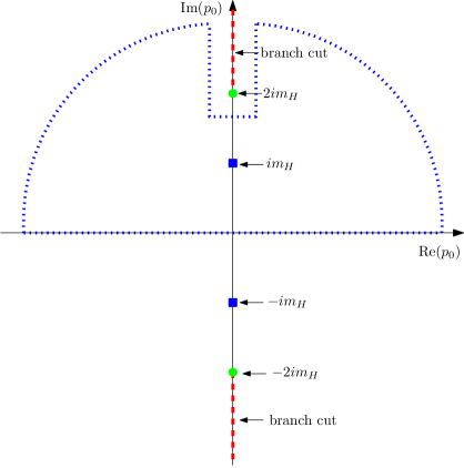
The main conclusions that can be drawn from this calculation are as follows. The propagator has a pole at by construction. In addition to that, it has a branch cut starting at . This branch cut will play a major role in the rest of this section. It is induced by the function appearing in Eq. (2.32). Here the branch cut of the square root in Eq. (2.31) was chosen to be located along the negative real axis. The resulting pole and branch cut structure of the Higgs propagator at zero spatial momentum is presented in Fig. 2.2a. Across the branch cut the real part of is continuous but the imaginary part has a discontinuity. It is remarked that the branch points of , which are given as , are not divergent singularities but only gaps in the definition domain of the propagator .
Since the physical decay width of a particle in Euclidean space-time and its mass are given through the real and imaginary part of the pole on the second Riemann sheet of the analytically continued propagator according to
| (2.34) |
for the case of the Higgs boson [44], the above calculation shows that the Higgs boson has zero decay width in the considered one-component -theory, and is thus a stable particle.
For clarification it is remarked that the first Riemann sheet of the propagator is given by Eq. (2.32). This function can be analytically continued across the branch cuts, where the propagator in Eq. (2.32) is discontinuous. The analytically continued function is then denoted as the propagator on the second Riemann sheet. In fact the analytical continuation depends on the side from which the branch cut is approached. These subtleties shall, however, not be discussed here. Due to the symmetries of the considered one-loop expression for the propagator in Eq. (2.32) they would result here only in adequate changes of the sign of the pole’s real and imaginary part in Eq. (2.34).
 |
 |
| (a) | (b) |
The preceding finding that the Higgs boson is stable in the one-component -theory is an obvious result, since there are no other particles present the Higgs boson could decay into. However, this situation changes completely if one considers the -theory with real components instead. In this extended theory one has one massive Higgs mode and massless Goldstone modes. However, the renormalized mass of the Goldstone modes is considered here as a free parameter to obtain a more general result for later use. Following the same steps as above, the Higgs propagator at one-loop order in the n-component -theory can be computed by calculating the one-Higgs-loop contribution and the one-Goldstone-loop contributions yielding
| (2.36) | |||||
| (2.37) |
where the factor comes again from the multiplicity of the considered diagrams and denotes the analytical continuation of onto the second Riemann sheet.
It is remarked that the renormalized quantities in Eq. (2.2) cannot be chosen independently of each other. This is clear from a physical perspective, since the latter quantities are connected to each other by emerging from the same set of bare parameters. In fact, the underlying theory is specified by only three bare parameters, namely , , and , while the propagator is parametrized here in terms of the five renormalized constants , , , , and which makes apparent the fact that the latter numbers, as emerging from the same underlying bare theory, must be related to each other, thus obeying additional constraints. Otherwise the renormalized result given in Eq. (2.2) would have more degrees of freedom than the underlying bare theory. Such constraints are parametrized in terms of the renormalization conditions which, however, have not explicitly been given yet. One constraint can, for instance, be inferred from the requirement that be real for purely positive values of , which is not automatically guaranteed by the general expression in Eq. (2.2), if all renormalized quantities could be chosen arbitrarily. Together with the later presented definition of the renormalized quartic coupling constant in Eq. (3.70) these constraints reduce the independent renormalized model parameters, for instance, to , , and , where would actually be zero in infinite volume. It is only kept as a free parameter here to obtain a more general result for later use. Conversely, the aforementioned constraints allow, for instance, for the perturbative calculation of the Higgs boson decay width, when the aforementioned independent quantities , , and are known, as will be discussed in chapter 8.
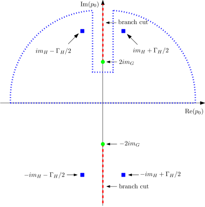
The branch and pole structure of the Higgs propagator in the considered n-component -theory at zero spatial momentum is presented in Fig. 2.2b. The main observation is, that the function induces a branch cut starting already at . This implies that the pole of the Higgs propagator can not be situated at purely imaginary values any longer, if the renormalized Goldstone mass is smaller than . Instead the pole is shifted away from the imaginary axis onto the second Riemann sheet of the analytically continued Higgs propagator. This is illustrated in Fig. 2.2b. In fact, there is a deep physical reason why the pole has to be shifted onto the second Riemann sheet and can not appear on the first sheet provided that the underlying Hamiltonian is hermitian. This consideration will be given at the end of this section.
The shifted pole thus leads to a non-zero decay width according to Eq. (2.34). This is the mathematical formulation of the expected result that the Higgs particle becomes unstable and can decay into pairs of Goldstone bosons provided that the quartic coupling constant is non-zero and that the Higgs boson mass is larger than the mass of the Goldstone pair, which is zero in infinite volume.
The signature of an unstable Higgs particle in Euclidean space-time is thus that the pole of the Higgs propagator has non-zero real and imaginary parts.This will play a role for the approaches to determine the Higgs boson mass in the later numerical calculations. Assuming the validity of the one-loop calculation the decay width can then be calculated from Eq. (2.2). However, the further discussion of the Higgs boson decay properties is postponed to chapter 8.
Moreover, it is remarked that extending this analysis to the Higgs-Yukawa model, including also the coupling to the fermion fields, yields very similar results. At one-loop order the fermion loop coupling to the Higgs boson induces again a branch cut starting at , where denotes here the renormalized mass of the considered fermion. This branch cut would again shift the pole of the Higgs propagator off the imaginary axis, provided that the renormalized Higgs boson mass is larger than . The obvious interpretation is that the Higgs particle is unstable and decays into pairs of the considered fermions, if , as expected.
Finally, the Euclidean time-correlation function of the Higgs field shall be discussed. This function will play an important role in the determination of the Higgs boson mass. It is defined as
| (2.38) | |||||
| (2.39) |
and can be calculated by closing the contour of the integral in Eq. (2.39) in the complex plane as illustrated in Fig. 2.2. For the case of the one-component -theory one then obtains
| (2.40) |
where the first term is induced by the residuum
| (2.41) |
of the Higgs propagator at its pole and the integral over the spectral function is given by the discontinuity of the Higgs propagator in Eq. (2.32) along the branch cut according to
| (2.42) |
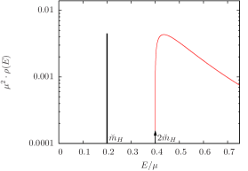
since its real part is continuous. The spectral function is thus real. From the result derived for the Higgs propagator in Eq. (2.32) one finds that is positive as illustrated in Fig. 2.3a for some specific choice of the renormalized parameters. The main conclusion for the one-component -theory is that the time correlation function is a sum of decaying exponential functions with purely positive weights. The argument of the slowest decaying exponential is given by the Higgs boson mass , which is clearly separated from the continuous spectrum described by the spectral function starting only at . In this scenario one can thus determine the Higgs mass by matching the time correlation function at large Euclidean time separations to a single exponential decay behaviour according to for .
This situation changes dramatically for the n-component -theory. Following the same steps as above one now finds for the time correlation function
| (2.43) |
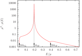
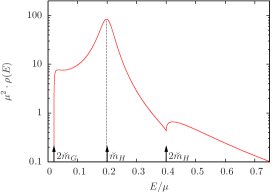
where the spectral function is again given by Eq. (2.42) but now based on the discontinuity of the Higgs propagator in Eq. (2.2). It is explicitly remarked that the poles of the Higgs propagator do not contribute to the contour integration, since they are only situated on the second Riemann sheet. They are therefore not within the integration contour, which is completely located on the first Riemann sheet. The main conclusion at this point is that the time correlation function is again given by a sum of decaying exponentials with positive weights, but in this case the spectral function of the exponential decay rates is completely continuously distributed as illustrated in Fig. 2.3b,c. In fact, there is no separated decay rate of the Higgs correlator in contrast to the previously discussed case of the one-component -theory.
 |
 |
 |
| (a) | (b) | (c) |
Conceptually, one can thus not apply the same procedure of matching to a single exponential behaviour at large Euclidean times to determine . However, as demonstrated in Fig. 2.3b for some specific choice of the renormalized parameters with a rather small value of the spectral function has a peak at and is completely dominated by that contribution in the presented setup. For sufficiently small values of the renormalized coupling constant the above procedure of determining thus remains applicable at least from a practical point of view. For larger values of on the other hand the peak at becomes less prominent. Therefore, the crucial observation is that analyzing the time correlation function in terms of a single exponential fit even at cannot be supposed to work well in the strong coupling regime. This will become an issue for the determination of the Higgs boson mass in the later numerical calculations.
It is remarked here that the above results are completely consistent with the equivalent picture in the operator formalism. In this approach the time correlation function of a given operator , depending only on field operators at the Euclidean time with being hermitian, is
where and denote the eigenvalues and the eigenvectors of the Hamiltonian . Provided that the Hamiltonian is hermitian, all eigenvalues are real and the time correlation function is a sum of decaying exponentials with positive weights. This is the reason why the pole of the Higgs propagator can not be situated on the first Riemann sheet if the Hamiltonian is hermitian. Otherwise there would be contributions of the corresponding residua to the time correlation function in Eq. (2.38) resulting in an oscillatory behaviour of which would be a contradiction to the result in Eq. (2.2).
2.3 Naive discretization of the Higgs-Yukawa sector on a space-time lattice
It was already noted in section 2.1 that the functional integrals in Eq. (2.1) and Eq. (2.11) are lacking a thorough mathematical definition in continuous space-time and that a sound definition of the integration measure can only be given for a discrete, finite set of space-time points . The given functional integrals therefore have actually to be understood as the limit of a high-, but finite-dimensional integration over the field variables with according to the integration measure given in Eq. (2.4) in the limit where the discrete points become infinitely densely packed and extends over the whole space-time. Moreover, discretized versions and of the actions and depending only on the field variables at the discrete points are required for this limit procedure and will be discussed later in this section.
Here, we continue with giving a precise meaning to the aforementioned limit procedure by specifying a particular form of the set of space-time points according to
| (2.45) |
which will be used in the following222The restriction that the given set only covers space-time points with non-negative coordinates would be trivially resolvable by adequate shifts of the specified coordinates. For the sake of brevity, however, we stay with the given expression.. This construction arranges the points in a hypercubic order and will thus be referred to as a lattice with side lengths and lattice spacing . Restricting ourselves to the consideration of the Euclidean functional integral in the following a well-defined meaning is then given to Eq. (2.11) by
| (2.46) | |||||
| (2.47) |
where the finite-dimensional (quasi) functional integral associated to the lattice is defined as
| (2.48) |
The inner limit in Eq. (2.46) will be referred to in the following as the infinite volume limit, while the outer limit will be called the continuum limit . It is, however, already remarked at this point that the notion of the ’continuum limit’ does actually not simply refer to sending the lattice spacing to zero. In fact, the bare coupling parameters have to be varied simultaneously in order to obtain a convergent result. This will be discussed in more detail in section 2.3.3. For the time being we continue here with using the notion ’continuum limit’ simply as a synonym for sending to zero.
It is exactly this definition of the functional integral that builds the basis of the so-called lattice approach. The lattice approach aims at calculating by the direct numerical evaluation of the right-hand side of Eq. (2.46). This is done by calculating for a series of different lattices with finite extent and non-zero lattice spacing . The obtained results have then to be extrapolated to the continuum and infinite volume limit in order to yield the correct result for .
A numerical method suitable for the evaluation of Eq. (2.46) on a finite space-time lattice will be discussed in section 3.5. In the following subsections we continue with the discussion of the discretized action , the choice of which is not unique and has a strong impact on the convergence properties of the limit procedure in Eq. (2.46). Besides that different lattice actions can also differ strongly with respect to the symmetries they obey. The latter observation will play a major role for the construction of the chirally invariant lattice Higgs-Yukawa model in section 3.3.
2.3.1 Discretization of the purely bosonic part of the action
In this section the discretization of the purely bosonic part of the Euclidean action given in Eq. (2.14) shall be discussed. Discretizing a continuous action is, however, not a unique procedure. The only strict requirement is that for any given set of smooth fields the discretized form of the action converges to its continuum counterpart in the limit . This rather loose condition leaves open much freedom for the construction of lattice actions, which can be used to improve the convergence properties of the lattice action in the aforementioned limit.
An obvious way to obtain a discretized version of the continuum action, that obeys the requirement to converge to its continuum counterpart, is given by replacing all differential operators with corresponding difference quotients of field variables at neighbouring lattice sites. Analogously, all space-time integrals would be represented as finite Riemann sums in this approach. Omitting the subscript indicating the Euclidean space-time from now on, this procedure applied to the purely bosonic part of the Euclidean action in Eq. (2.14) yields
| (2.49) |
where the unspecified summation over the space-time points is always meant to be performed over the set of lattice points in the following and the summation over runs over the four unit basis vectors along the four Euclidean space-time dimensions. The applied lattice forward derivative operator in direction is defined as
| and | (2.50) |
where denotes the corresponding backward derivative. At the boundary of the space-time point may leave the set and the field variable would be undefined. In that case an appropriate modulo operation according to is implicitly assumed here. The lattice is then said to have periodic boundary conditions.
In the given lattice action the nearest neighbour forward difference quotient has been chosen to substitute the differential operator. The discretization error of this lattice operator is known to be of order . However, the total error term of the given lattice action only starts at . This is because the lattice sum over the given product of difference quotients can be rewritten in terms of the symmetric, second derivative difference quotient expression according to
| (2.51) |
the discretization error of which is of order . Furthermore, due to the aforementioned periodicity of the lattice the Riemann sum in Eq. (2.49) corresponds to a trapezoidal rule [127] approximating the targeted integral in continuous space-time with an error term starting at . The total discretization error of the given lattice action is thus of order .
However, the order of the discretization error of the discretized action alone does not specify the order of the discretization error that one will encounter in the evaluation of a specific observable. The reason for that is twofold. First of all the considered discretized observable itself may contain deviations from its continuum counterpart with different order in than the discretization error of the action. This applies at least to all observables containing differential operators, such as the topological charge observable in lattice QCD, since the aforementioned differential operators contained within such observables have to be discretized as well. Secondly, and more interestingly, the integration over all field configurations in the functional integral in Eq. (2.48) generates additional contributions to the expectation value of the considered observable that would not be present in the continuum, and these disturbing contributions can be of lower order in the lattice spacing than the lowest order discretization error observed in the lattice action or in the discretization of the considered observable itself. In general, all possible terms that have the same dimension as the considered observable and that are not prohibited by the symmetries simultaneously obeyed by the theory and the considered observable can be generated in this way, i.e. by quantum fluctuations. This was first discussed in the famous work of Symanzik introducing the Symanzik improvement program [128, 129].
The main idea of the Symanzik improvement program is to identify all terms that can potentially be generated in the functional integral, i.e. all terms that are compatible with the symmetries of the model, and to add corresponding counterterms with appropriately chosen coefficients to the underlying action, such that all unwanted terms of a certain order in the lattice spacing are exactly canceled.
The analysis of the purely bosonic lattice theory specified through Eq. (2.49) shows that parity and time reflection symmetry greatly constrain the terms that can be generated by quantum fluctuations, provided that the considered observable also obeys these symmetries. In that case, one finds that discretization errors can only have even powers in the lattice spacing [128, 129]. The lowest order of a possible discretization error is thus .
With the apparatus of the Symanzik improvement program at hand it is possible to construct improved lattice actions such that the observables of interest have even better convergence orders than . However, since the fermionic part of the lattice action that will actually be used in the later calculations is of order , we will stay with the expression given in Eq. (2.49).
Finally, the eigenvectors and eigenvalues of the lattice derivative operator shall be introduced for later use. As in the continuum the eigenvectors are given by plane waves, the allowed four-component momenta of which, however, are restrained to the set of lattice momenta
| (2.52) |
associated to the set of lattice points . The corresponding eigenvalues are then given by the squared lattice momenta according to
| (2.53) |
with
| (2.54) |
In the non-interacting case the lattice propagator of the bosonic field in momentum space
| (2.55) |
with can then be written in terms of the aforementioned eigenvalues according to
| (2.56) |
where the field variables in momentum space are given as
| (2.57) |
with denoting the lattice volume.
The concluding remark at this point is that the obtained lattice propagator and in particular the location of its pole deviate from their continuum results by discretization errors starting at order , as expected. One also learns from the appearance of the term in Eq. (2.56) that Lorentz-symmetry, which becomes an -symmetry in Euclidean space-time is explicitly broken by the lattice, as expected. However, the latter symmetry is finally restored in the continuum limit and the symmetry breaking terms disappear rather quickly at order .
2.3.2 Naive discretization of the fermionic part of the action
Following the same straightforward ansatz, which worked satisfactorily for the case of the purely bosonic part of the action, a first approach to a lattice formulation of the Euclidean fermion action given in Eq. (2.1) would be
An obvious disadvantage of this discretization is its rather bad convergence behaviour in the limit due to the discretization error of the given action being of order as induced by the non-symmetric lattice derivative operator . The most severe problem with this approach, however, is more subtle. The application of the non-symmetric lattice derivative operator breaks explicitly reflection positivity such that the hermiticity of the Hamiltonian associated to the discrete system, and thus the positivity of the so-called transfer matrix being the matrix representation of the transfer operator , is no longer guaranteed [130, 98]. Moreover, it could be generally shown within the framework of QED that any application of a non-symmetric form of a lattice derivative operator for the discretization of the fermionic action leads to the emergence of non-covariant terms in the fermion self-energy and other observables in the continuum limit [130]. This is a severe defect, since the continuum physics would not be correctly reproduced in the continuum limit .
This severe problem can be cured by replacing the non-symmetric lattice derivative operator with the symmetrized, anti-hermitian operator defined as
| (2.59) |
which does not break reflection positivity. Moreover, the discretization error of the symmetric operator only starts at order . At tree-level the lattice artefacts of the resulting fermion action itself are thus of order . As discussed in the previous section, it is not guaranteed that this apparent tree-level -improvement also holds when quantum fluctuations are considered. In fact, a detailed analysis for the case of QCD following the ideas of the Symanzik improvement program [128, 129] shows that the apparent -improvement is indeed broken at the quantum level. If quantum corrections are respected in this analysis, one finds that the discretization errors actually start at order in the interacting case [131]. -improvement can then only be achieved by a modification of the fermion lattice action. It was found that at least on-shell -improvement can be established through the extension of the action by the so-called Sheikholeslami-Wohlert term [131].
Here, however, we will no further address the question of the convergence properties of the introduced fermion action in the continuum limit, since it will be seen shortly, that it actually suffers from a more severe defect. This defect becomes most obvious when considering the fermion propagator in momentum space, which is given as
| (2.60) |
with
| and | (2.61) |
where selects the quark flavour, and denote the Fourier transforms of the respective quark fields, is a matrix, and is a four-component lattice momentum. For the massless case in the non-interacting theory the fermion propagator is easily obtained by the rules of Grassmann integration yielding
| (2.62) |
where denotes the eigenvalue of the symmetrized lattice derivative associated to the eigenvector according to
| with | (2.63) |
The main observation is that the free lattice propagator matches its continuum counterpart for small momenta, since one has in the continuum limit . In particular, the propagator in Eq. (2.60) has a pole at in agreement with the considered fermion being massless. However, the additional zeros of the sine at the edges of the Brillouin zone induce 15 additional poles in the propagator that give contributions to any computed observable as if there were 15 additional fermions present in the theory. This phenomenon is called ’fermion doubling’ and is directly related to the application of the symmetrized derivative operator, which had to be chosen due to the aforementioned constraints.
A widely spread approach aiming at the suppression of the contributions of the unwanted fermion doublers in the continuum limit is the introduction of the so-called Wilson term into the fermion lattice action. Adopting this strategy to the Higgs-Yukawa model the fermion lattice action becomes
with the pioneering Wilson Dirac operator given as
| (2.65) |
where the so-called Wilson parameter is usually chosen as , which is a reasonable choice as discussed in LABEL:Sheikholeslami:1985ij.
The effect of the Wilson term can again most obviously be studied by considering the free fermion propagator, which now becomes
| (2.66) | |||||
| (2.67) |
The free propagator still has 15 additional, unphysical poles. The corresponding quasi particles, however, have now acquired a mass given by a constant times . In the continuum limit the unwanted fermion doublers thus become infinitely massive and their contribution to any observable vanishes.
The inclusion of the Wilson term thus solves the fermion doubling problem. The price one pays when adopting this approach is twofold. Most obviously, the inclusion of the Wilson term induces lattice artefacts already at tree-level. More interesting from a conceptual point of view is, however, the loss of chiral symmetry, meaning that the standard chiral symmetry relation
| (2.68) |
where is some Dirac operator does not hold for the Wilson Dirac operator , since the Wilson-term does not anti-commute with .
In fact, the celebrated Nielsen-Ninomiya-theorem [132, 133, 134, 135] excludes the possibility of constructing a real, bilinear lattice fermion action that is local and translational invariant while obeying the chiral symmetry relation in Eq. (2.68) and lifting the unwanted fermion doublers at the same time. Any approach of investigating chiral symmetry on the lattice thus has to abandon at least one of the aforementioned requisites. This will be discussed in more detail in section 3.1.
2.3.3 Continuum limit
As already pointed out the notion ’continuum limit’ does not simply refer to sending the lattice spacing to zero. In fact, physical observables in interacting theories do not even converge to finite results in general, when the lattice spacing is sent to zero, while the bare parameters are held constant. This observation is closely connected to the general appearance of infinities in bare perturbation theory of unregulated, interacting theories, since the introduction of a finite spaced lattice is nothing else but a regularization of the considered theory and the limit directly corresponds to its removal. This lattice regularization restricts the set of respected momenta to the allowed lattice momenta given in Eq. (2.52). The lattice spacing is thus manifestly related to a momentum cutoff parameter .
To avoid confusion it is remarked that the lattice regularization does not exactly correspond to a hard momentum cutoff. While the discrete lattice momenta themselves are nominally cut off at the edges of the Brillouin zone according to , their respective contribution to physical observables already deviates from the targeted continuum contribution at significantly smaller momenta, which becomes apparent, for instance, in the analytical expressions for the bare fermion and bosonic propagators considered in the preceding sections. In this respect the nominal threshold value can actually not be considered as a hard momentum cutoff and a physically meaningful cutoff parameter can in fact not uniquely be defined. Instead, only its scale is physically meaningful. Here and in the following we will choose the definition of the cutoff parameter to be . The underlying ambiguity, however, will later become an issue when trying to compare the eventually derived cutoff-dependent mass bounds with results obtained in other regularizations.
To establish a meaningful continuum limit the bare parameters thus have to be varied along with sending the lattice spacing to zero. Following the Wilsonian picture of renormalization [136], this can be achieved by choosing a number of linearly independent physical observables equal to the number of bare parameters available in the considered theory, the expectation values of which are kept constant by suitable adjustments of the bare parameters, while sending the lattice spacing to zero. Through this procedure one defines trajectories of constant physics in terms of the selected physical observables in bare parameter space spanned by the bare parameters and the lattice spacing .
While the tuned expectation values converge to finite values with by construction, provided that the aforementioned trajectories exist at all and can be extended down to arbitrarily small lattice spacings , such a convergent behaviour is not automatically guaranteed for all other observables. In fact, this is a property of the considered theory. For the purpose of categorization, the notion of ’non-perturbative renormalizability’ refers to all those theories, in which for any point in bare parameter space a trajectory of constant physics can be constructed by a suitable choice of and extended down to arbitrarily small lattice spacings , such that the expectation values of all physical observables - not only of the tuned ones - converge to finite values when sending the lattice spacing to zero along the constructed trajectory. In such a non-perturbatively renormalizable theory a meaningful continuum limit can thus be established by adjusting the bare parameters to a trajectory of constant physics while sending .
In order to extract actual continuum physics as observed in Nature one would moreover have to select that specific trajectory of constant physics that reproduces phenomenology. This is done in practice by tuning the expectation values of the selected observables to their respective phenomenologically known values.
In the case of the pure Higgs-Yukawa sector one has four free bare parameters at hand for a given lattice spacing , if one respects only the heaviest fermion doublet, i.e. the top-bottom doublet. These are the top and bottom Yukawa coupling constants , , the scalar mass and the quartic self-coupling constant . The phenomenologically relevant trajectory of constant physics can then, for instance, be constructed by tuning these bare parameters to reproduce the phenomenological top and bottom quark masses, the phenomenological value of the vev, and a constant Higgs boson mass. Since the Higgs boson mass is not determined yet, a one-dimensional freedom in the fixation of the phenomenologically relevant trajectory is left open, which can, for instance, be parametrized in terms of the quartic self-coupling parameter at a given lattice spacing . This is exactly the approach that will be applied in the present work.
For clarification it is remarked that the pure Higgs-Yukawa sector of the Standard Model is actually not considered as a non-perturbatively renormalizable theory due to the triviality of the Higgs sector, meaning that the trajectories of constant physics can not be extended to arbitrary small . The lattice spacing , and thus the cutoff , can therefore not be removed from the theory and any physical results thus have to depend on this scale. This is the mathematical manifestation of the Higgs-Yukawa sector being an effective theory only valid up to some cutoff . The strategy for the extraction of the cutoff dependent results is nevertheless the same, which is to construct trajectories of constant physics compatible with phenomenology and to extend them as far as possible. The cutoff dependent result is then taken from the constructed trajectory at the specified value of the cutoff , i.e. at the specified lattice spacing .
In a practical implementation, however, it is useful to exploit the fact that all appearances of the lattice spacing can be completely removed from the evaluation of the functional integral in Eq. (2.48) through a rescaling of the field variables and bare parameters according to
| (2.69) | |||||
| (2.70) |
The expectation value of the dimensionless observable , from which the actually targeted expectation value can directly be obtained by a trivial rescaling, is then given by the dimensionless expression
| (2.71) |
where the functional integral is defined as
| (2.72) |
In the above equation the total action is expressed in terms of the rescaled quantities according to
| (2.73) | |||||
where the dimensionless lattice operators are given as
| (2.75) |
The technical advantage that arises from the fact that the lattice spacing can be removed by introducing a set of rescaled fields and bare parameters is that the required tuning of the bare parameters, as described above, becomes simplified. This is because the lattice spacing can directly be reintroduced into the dimensionless system in Eq. (2.71) by demanding that one expectation value of the selected observables, for instance , exactly matches its phenomenological value. Practically speaking, one then only needs to fine-tune the bare parameters with respect to the reduced set of the remaining conditions, matching to their phenomenological values. In the case of the considered Higgs-Yukawa sector one can, for instance, reintroduce the lattice spacing by demanding the vev to match its phenomenologically known value of . The remaining task would then be to fine-tune the Yukawa coupling constants to reproduce the physical quark masses, while the bare quartic coupling constant would stay a free parameter, as discussed above. This procedure will be presented in more detail in section 3.4.
For practical lattice calculations it is therefore very convenient to consider the dimensionless expression given in Eq. (2.71), which will be the actual starting point of the later lattice computations. The construction of the above described continuum limit then requires the existence of a critical point in the dimensionless system where all correlation lengths diverge. Such a critical point is necessary to allow for holding the physical observables constant in the limit according to the underlying scaling relations in Eq. (2.69-2.70). The same reasoning moreover requires the associated phase transition to be of second order. Knowing the phase structure of the considered model is therefore an important prerequisite for the construction of the continuum limit. For the later introduced lattice Higgs-Yukawa model the phase structure will therefore be investigated in detail in chapter 4.
Chapter 3 The chirally invariant lattice Higgs-Yukawa model
As pointed out in the introduction the earlier non-perturbative investigations of lattice Higgs-Yukawa models suffered from their inability to restore chiral symmetry in the continuum limit while lifting the unwanted fermion doublers at the same time. Since then, however, several new approaches for the construction of chirally invariant lattice fermions have been developed [137, 138, 139, 140, 78]. These new fermion formulations allow for a consistent formulation of the chiral Higgs-fermion coupling structure of the Standard Model on the lattice while simultaneously lifting the fermion doublers, thus eliminating manifestly the main objection to the earlier investigations.
The lattice Higgs-Yukawa model that is investigated in the present work is based on the Neuberger overlap operator [139, 140] which is a solution of the Ginsparg-Wilson relation [79]. The properties of this operator will be briefly discussed in section 3.1. The first chirally invariant lattice Higgs-Yukawa model, obeying an lattice chiral symmetry, was originally introduced by Lüscher [78]. It will be presented in section 3.2 in some reformulation being intuitively better accessible. Based on these considerations it is a small step to establish the Higgs-Yukawa model that will actually be studied in this work obeying a lattice chiral symmetry. This will be done in section 3.3.
The main strategy for approaching the eventual aim of the present work, which is the non-perturbative determination of upper and lower Higgs boson mass bounds, will be discussed in section 3.4. Most of the observables investigated in the rest of this thesis are also explicitly defined there.
A first account on the lattice techniques used to evaluate the considered Higgs-Yukawa model numerically is then given in section 3.5. Serving as a starting point for the numerous algorithmic enhancements, which will be presented in detail in chapter 5, a standard implementation of an HMC-algorithm [141, 142] is given at that point, which will also extensively be used in chapter 4 for the numerical evaluation of the phase diagram of the considered Higgs-Yukawa model.
For the later numerical treatment of the model the properties of the fermion determinant play a vital role, in particular the question, whether and, if yes, how much its complex phase fluctuates during the Markov process of generating field configurations. The complex phase of the fermion determinant associated to the considered Higgs-Yukawa model is therefore discussed in section 3.6.
3.1 The chirally invariant Neuberger Dirac operator
It is well known that the Nielsen-Ninomiya-theorem [132, 133, 134, 135] excludes the possibility of constructing a real, bilinear lattice fermion action that is local and translational invariant while obeying the standard chiral symmetry relation given in Eq. (2.68) and lifting the unwanted fermion doublers at the same time. Any approach of investigating chiral symmetry on the lattice thus has to abandon at least one of the aforementioned requisites.
A nowadays very commonly used ansatz for studying chiral properties on the lattice is based on the observation [79] that the Nielsen-Ninomiya-theorem can be circumvented by replacing the continuum chiral symmetry in Eq. (2.68) with a lattice modified version thereof, that recovers the actual symmetry only in the continuum limit. The construction of lattice theories exactly obeying this modified chiral symmetry is then not excluded by the Nielsen-Ninomiya-theorem. The great advantage of this approach lies in the existence of an exactly preserved symmetry established at any lattice spacing even far away from the continuum limit. It is the form of this exact symmetry itself that converges to the continuum chiral symmetry in the continuum limit.
More precisely, it was found that any operator that satisfies the Ginsparg-Wilson relation [79]
| (3.1) |
where denotes the lattice spacing and is some hermitian, positive definite operator, being local in position space and proportional to the identity in Dirac space, then obeys the lattice modified chiral symmetry relation
| (3.2) |
with the modified -matrix
| (3.3) |
It can directly be seen from the appearance of the lattice spacing on the right hand side of Eq. (3.3) that converges to in the continuum limit, thus recovering the continuum chiral symmetry for and one easily verifies that any operator of the form
| (3.4) |
solves the Ginsparg-Wilson relation in Eq. (3.1) provided that the operator satisfies
| and | (3.5) |
This, however, does not guarantee the resulting Dirac operator to be free of fermion doublers.
A specific solution of the Ginsparg-Wilson relation for which it could explicitly be shown that it lifts the unwanted fermion doublers was presented in LABEL:Neuberger:1998wv. This so-called Neuberger overlap operator is given as
| (3.6) |
where is a free, dimensionless parameter within the specified constraints that is related to the operator in Eq. (3.1) through and denotes here the Wilson operator as defined in Eq. (2.65). Furthermore, the given operator was proven to be local in a field theoretical sense also in the presence of QCD gauge fields which, however, are not considered here, at least if the latter fields underlying the considered Dirac operator obey certain smoothness conditions [143]. The locality properties were then found to depend on the parameter and the strength of the gauge coupling constant [143]. At vanishing gauge coupling the most local operator was shown to be obtained at . Here, the notion ’most local’ has to be understood in the sense of the most rapid exponential decrease with the distance of the coupling strength induced by the matrix elements between the field variables at two remote space-time points and . For that reason the setting will be adopted for the rest of this work.
The locality properties, the successful lifting of the unwanted fermion doublers and the existence of an exact, though modified, chiral symmetry make the Neuberger operator an excellent candidate for the construction of chiral theories on the lattice. The downside of this operator, however, are the tremendous numerical costs required for its application on a given vector, which mainly result from the appearance of the inverse square root of the hermitian operator in Eq. (3.6). Much effort has therefore been spent on developing more efficient algorithms for performing lattice calculations with dynamical fermions based on the Neuberger overlap operator [144, 145, 146, 147].
In the present work aiming at the investigation of the pure Higgs-Yukawa sector, however, the situation is much different, since no gauge fields are included in this sector of the Standard Model. It is the absence of gauge fields that makes the eigenvectors and eigenvalues of the Neuberger operator analytically available. In momentum space with the allowed four-component momenta the eigenvectors of the doublet Dirac operator that will actually be used in the construction of the Higgs-Yukawa model in the following are given as
| (3.7) |
with denoting the usual four-component spinor structure
| (3.8) |
where the lattice momenta have been defined in Eq. (2.63). Here are two orthonormal vectors and the four component quaternionic vectors , are defined as and with denoting the vector of Pauli matrices. The corresponding eigenvalues are then given as
| (3.9) |
where the squared lattice momenta have been given in Eq. (2.54). Here denotes the coefficient of the Wilson term in the underlying Wilson Dirac operator and equals the sign of the imaginary part of the complex eigenvalues according to . The eigenvalues thus form a circle in the complex plane, the radius of which is given by the parameter .
It is this analytic availability of the eigenvalues and eigenvectors that allows for an extremely efficient construction of the Neuberger overlap operator in momentum space as will be discussed in section 3.5.
3.2 A first lattice Higgs-Yukawa model
The first formulation of a chirally invariant lattice Higgs-Yukawa model has been given by Lüscher [78]. It was shown in that work that a chirally invariant lattice theory can be constructed starting from any Dirac operator that satisfies the Ginsparg-Wilson relation in Eq. (3.1) and that the resulting model is free of fermion doublers at least for sufficiently small coupling constants provided that the underlying Dirac operator possesses that property. This first formulation of an chirally invariant lattice Higgs-Yukawa model was given as111With some abuse of notation the specification of the partition function is taken here and in the following as a shorthand notation for defining a lattice model. More precisely one would have to specify the functional integral in terms of which the expectation value of an observable is given according to , .
| (3.10) | |||||
| (3.11) | |||||
| (3.12) |
where denotes a one-component complex scalar field, is the Yukawa coupling constant, and , are Dirac fields. The left- and right-handed projection operators are moreover given in the usual manner according to
| (3.13) |
The Higgs action is not further specified, except for the requirements that it solely depends on the field and that it is invariant under global transformations of the scalar field . The lattice -action would thus be an eligible candidate for . The particular choice of the Dirac operator is also left open with the only requirement of being a solution to the Ginsparg-Wilson relation.
For clarification it is remarked that the field does not propagate and that it does not have any physical interpretation at all. It was only introduced in LABEL:Luscher:1998pq as an auxiliary tool facilitating the construction of the chirally invariant coupling structure among the fermionic and bosonic fields. This auxiliary field is introduced here in such a way that the sum transforms according to the continuum chiral symmetry.
One can then easily verify that this model obeys a global symmetry as well as an exact, but lattice modified, chiral symmetry according to
| (3.14) | |||||
| (3.15) |
where is some infinitesimally small parameter. The given symmetry then recovers the actual continuum symmetry in the limit .
A more enlightening representation of the partition function given in Eq. (3.10) can be obtained by integrating out the fermion fields and leading to
| (3.16) |
up to a constant factor. Here the expressions and have actually to be understood as the space-time-diagonal matrix and . This type of shorthand notation will extensively be used in the following. Starting at the given representation one can make the left- and right-handed coupling structure of the theory more explicit and thus intuitively better understandable by defining the modified left- and right-handed projection operators as well as the modified -matrix according to
| (3.17) |
Employing the Ginsparg-Wilson relation these modified operators can be shown to satisfy the relations
| (3.18) |
and
| (3.19) |
allowing to rewrite the partition function after reintroducing the fermion fields , in the equivalent222The notion of two partition functions and being equivalent expresses that the expectation values of any observable determined by the functional integrals , associated to the given partition functions according to and are identical. Here the partition function in Eq. (3.20) is equivalent to the one in Eq. (3.10), if one restricts the consideration to physical observables, i.e. observables not depending on . Analogously, this notion of equivalence is also used for the underlying actions and . but physically more enlightening form
| (3.20) | |||||
| (3.21) |
which no longer contains the auxiliary field . The obvious physical interpretation of this model is that the left- and right-handed modes of the field are given here by the expressions and based on the modified projection operators, while the left- and right-handed modes of are still defined via the original projection operators [80, 81].
Finally, the chiral symmetry of the model can also be written in a more enlightening form exploiting the definition of the above projection operators. One finds that the model is invariant under the transformation
| (3.22) | |||||
| (3.23) |
where are arbitrarily chosen.
3.3 The definition of the lattice Higgs-Yukawa model
The model that will actually be considered in the following, is a four-dimensional, chirally invariant lattice Higgs-Yukawa model based on the Neuberger overlap operator, aiming at the implementation of the chiral Higgs-fermion coupling structure of the pure Higgs-Yukawa sector of the Standard Model reading
| (3.24) |
with and denoting the bare top and bottom Yukawa coupling constants. In this model the consideration is restricted to the top-bottom doublet interacting with the complex Higgs doublet , which is a reasonable simplification, since the Higgs dynamics is dominated by the coupling to the heaviest fermions.
The fields considered in this model are one four-component, real scalar field , being equivalent to the complex doublet of the Standard Model, and top-bottom doublets represented by eight-component spinors , . In this work, the chiral character of the targeted coupling structure in Eq. (3.24) will be preserved on the lattice by constructing the fermionic action from the (doublet) Neuberger overlap operator which will, however, be denoted as in the following for the sake of brevity. Starting directly from the formulation in Eq. (3.21) one can write down a chirally invariant lattice Higgs-Yukawa model according to
| (3.25) | |||||
| (3.26) |
where the four-component scalar field , defined on the Euclidean site indices of a -lattice, was rewritten as a quaternionic, matrix with denoting the vector of Pauli matrices, acting on the flavour index of the fermion doublets. Here and in the following the lattice spacing is assumed to be . The lattice spacing can later be reintroduced as discussed in section 2.3.3. According to the more general definition in Eq. (3.17) the modified left- and right-handed projection operators associated to the Neuberger Dirac operator are given as
| (3.27) |
where the free parameter of the overlap operator will be set to one in the actual implementation of the model as discussed in section 3.1. This action now obeys an exact global lattice chiral symmetry. For and the action is invariant under the transformation
| (3.28) | |||||
| (3.29) |
with denoting the respective representations of the global symmetry group. Employing the explicit form of the hypercharge being related to the isospin component and the electric charge according to , the above matrices can explicitly be parametrized as
| (3.36) |
for the case of the considered top-bottom doublet. For clarification it is remarked that the right-handed fields are isospin singlets and have only been written here in form of doublets for the sake of a shorter notation. Note also that in the mass-degenerate case, i.e. , the above global symmetry is extended to . In the continuum limit the symmetry in Eq. (3.28-3.29) recovers the continuum global chiral symmetry and the lattice Higgs-Yukawa coupling becomes equivalent to Eq. (3.24) when identifying
| (3.41) |
for some real, non-zero constant .
The formulation in Eq. (3.25-3.26) is helpful for identifying the chiral symmetries of the model. For its further treatment, however, the fermion degrees of freedom have to be integrated out. This can explicitly be done by the rules of Grassmann integration. The expectation value of some observable is then obtained as
| (3.42) |
where the remaining functional integral over the field is given as
| (3.43) | |||||
| (3.44) |
with the effective action being
| (3.45) | |||||
| (3.46) |
With the help of Eq. (3.19) the fermion matrix appearing in the above equations can then be written as
| (3.47) | |||||
| (3.48) | |||||
| (3.49) | |||||
| (3.50) | |||||
| (3.51) |
where this rather fragmentary presentation was chosen here to establish the notation that will be used in the forthcoming analytical considerations. It is remarked that the observable is different from in general and depends only on the scalar field . Its specific form has to be worked out by the rules of Grassmann integration, leading then to the potential appearance of matrix elements of the inverse fermion matrix in the respective expression for . It is also remarked, that the symmetry with respect to the transformation of the scalar field given in Eq. (3.28-3.29) is directly inherited to the determinant . Further properties of the latter determinant, in particular the behaviour of its potentially complex phase will be addressed in section 3.6.
The so far unspecified purely bosonic action is chosen here to be the lattice -action parametrized by the hopping parameter and the lattice quartic coupling constant according to
| (3.52) |
which is a convenient parametrization for the actual numerical computations. However, this form of the lattice action is fully equivalent to the lattice action in continuum notation given in Eq. (2.49) written in terms of the bare mass , the bare quartic coupling constant , and the lattice derivative operator . The connection is established through a rescaling of the scalar field and the involved coupling constants according to
| (3.53) |
In the given model the expectation value would always be identical to zero due to the symmetries in Eq. (3.28-3.29). To study the mechanism of spontaneous symmetry breaking, one usually introduces an external current , which has to be removed after taking the thermodynamic limit, leading then to the existence of symmetric and broken phases with respect to the order parameter as discussed in section 2.1. In this scenario the bare vev is directly given by in the limit . An alternative approach, which was shown to be equivalent in the thermodynamic limit [148, 149, 124], is to define the vev as the expectation value of the rotated field given by a global transformation of the original field according to
| (3.54) |
with the matrix selected for each configuration of field variables such that
| (3.55) |
Here we use this second approach. According to the notation in Eq. (2.49), which already includes a factor , the relation between the vev and the expectation value of is then given as
| (3.56) |
In this setup the unrenormalized Higgs mode and the Goldstone modes can directly be read out of the rotated field according to
| (3.57) |
The great advantage of this approach is that no limit procedure has to be performed, which simplifies the numerical evaluation of the model tremendously. It is finally remarked that from now on we can assume the degeneracy of the vacua to be broken whenever we consider analytical calculations due to the equivalence of this technique with the explicit introduction of an external current .
3.4 Simulation strategy and considered observables
The eventual aim of this work is the non-perturbative determination of the cutoff dependent upper and lower bounds of the Higgs boson mass as defined in Eq. (2.34). The general strategy that will be applied for that purpose is the non-perturbative evaluation of the whole range of Higgs boson masses that are attainable within the pure Higgs-Yukawa sector at a fixed value of the cutoff in consistency with phenomenology. This will be done by numerically evaluating the finite lattice model of the Higgs-Yukawa sector introduced in the preceding section and extrapolating the obtained results to the infinite volume limit.
As discussed in section 2.3.3 the requirement of reproducing phenomenology restricts the freedom in the choice of the bare parameters due to the phenomenological knowledge of the renormalized quark masses and the renormalized vacuum expectation value of the scalar field. Throughout this work , , and will be assumed333In its current listing [10] the Particle Data Group specifies in the scheme, as the perturbative top pole mass, and , where the Fermi coupling constant is related to the renormalized vev through . However, due to the ambiguity of the latter quark masses with respect to the chosen renormalization scheme, and since statistical and systematic errors will dominate the uncertainty of the finally obtained results in this work, it is not so meaningful to adopt the most recent results on the aforementioned quantities for the intended lattice calculations. Instead, the settings given in the main text were taken over from prior Higgs-Yukawa model investigations [73].. Here , , and denote the renormalized top and bottom quark masses as well as the renormalized vev in dimensionless lattice units. However, these conditions leave open an one-dimensional freedom in the bare parameters, which will be addressed at the end of this section.
Furthermore, the model has to be evaluated in the broken phase to respect the observation of spontaneous symmetry breaking, however close to a second order phase transition to a symmetric phase as discussed in section 2.3.3.
The physical scale, i.e. the inverse lattice spacing , can then be reintroduced by comparing the renormalized vev measured on the lattice with its phenomenologically known value according to
| (3.58) |
where denotes the Goldstone renormalization constant. Associated to the lattice spacing is a cutoff parameter of the underlying lattice regularization, which is defined here as
| (3.59) |
As already pointed out in section 2.3.3, this definition is not unique, and other authors use different definitions, for instance motivated by the value of the momenta at the edge of the Brillouin zone. However, since the quantities that actually enter any lattice calculation are rather the lattice momenta instead of the momenta , which are connected through the application of a sine function according to Eq. (2.63), it seems natural to choose the definition of the cutoff given in Eq. (3.59).
In the Euclidean continuum the aforementioned Goldstone and Higgs renormalization constants, more precisely their inverse values and , are usually defined as the real part of the derivative of the inverse Goldstone and Higgs propagators in momentum space with respect to the continuous squared momentum at some scale and , respectively. The restriction to the real part is introduced to make this definition applicable also in the case of an unstable Higgs boson, due to the branch cut structure of the propagators at negative values of induced by the massless Goldstone modes as discussed in section 2.2. This is the targeted definition that shall be adopted to the later lattice calculations.
On the lattice, however, the propagators are only defined at the discrete lattice momenta according to
| (3.60) | |||||
| (3.61) |
where the Higgs and Goldstone fields in momentum representation read
| and | (3.62) |
with denoting the lattice volume.
Computing the derivative of the lattice propagators is thus not a well-defined operation. Moreover, the lattice propagators are not even functions of , since rotational invariance is explicitly broken by the discrete lattice structure. To adopt the above described concept to the lattice nevertheless, some lattice scheme has to be introduced here that converges to the continuum definitions of and in the limit . The idea is to use some analytical fit formulas , derived from renormalized perturbation theory in the Euclidean continuum to approximate the measured lattice propagators and at small momenta for some appropriate value of such that the discretization errors are acceptable. The details of this fit procedure are discussed in section 6.1 and section 7.1. One can then define the analytically continued lattice propagators as
| and | (3.63) |
The targeted Goldstone and Higgs renormalization constants and can then be defined444Exploiting the -symmetry of the continuous propagators one has with some abuse of notation, where an underlying mapping is implicitly assumed. as
| (3.64) | |||||
| (3.65) |
A natural choice for the fixation of the scales , is the so-called on-shell scheme, where one sets the scales , to the squared masses , of the Higgs and Goldstone bosons. As already discussed in section 2.2 the physical masses are given by the poles of the respective propagators on the second Riemann sheet. To adopt this definition to the introduced lattice scheme we define the Higgs boson mass , its decay width , and the mass of the stable Goldstone bosons through
| and | (3.66) |
where denotes the analytical continuation of onto the second Riemann sheet.
Extracting the Higgs mass and its decay width according to this definition would, however, require a very accurate analytical continuation of the Higgs propagator onto the second Riemann sheet. While such a continuation can in principle be obtained with the help of a decent fit formula as will be discussed in more detail in section 6.1 and section 7.1, reaching the necessary level of accuracy to extract the mass and the decay width reliably from Eq. (3.66) is a highly non-trivial task. Such an analytical continuation will nevertheless later be tried.
Owing to these difficulties the Goldstone and Higgs renormalization factors are rather determined at the scales and given by the masses and , which will be referred to in the following as propagator masses in contrast to the pole masses and . We thus define
| and | (3.67) |
where the propagator masses , are defined through a vanishing real-part of the inverse propagators according to
| and | (3.68) |
The reasoning for selecting these latter definitions for the Higgs and Goldstone masses is, that the required analytical continuation in the case of the Higgs propagator is much more robust, since it only needs to extend the measured lattice propagator to purely negative values of in contrast to the situation resulting from the definition in Eq. (3.66). It is remarked here that the Goldstone propagator mass was only introduced for the sake of an uniform notation, since is identical to , due to the Goldstone bosons being stable.
As for the unstable Higgs boson, however, one finds that the discrepancy between the pole mass and the propagator mass is directly related to the size of the decay width . In the weak coupling regime of the theory the two mass definitions and can thus be considered to coincide up to small perturbative corrections, due to a vanishing decay width in that limit. For the pure -theory the deviation between and has explicitly been worked out in renormalized perturbation theory [44]. In infinite volume the finding is
| (3.69) |
where denotes the renormalized quartic self-coupling constant and is the number of components of the scalar field , i.e. for the here considered case. This calculation was performed in the pure -theory, thus neglecting any fermionic degrees of freedom, and for exactly massless Goldstone particles. However, one learns from this result that the definition of in Eq. (3.68) as the Higgs boson mass is very reasonable at least for sufficiently small values of the renormalized coupling constants.
The definition of the renormalized quartic self-coupling constant that was used in the derivation of Eq. (3.69) is
| (3.70) |
which shall also be taken over to the considered Higgs-Yukawa model. It is remarked, that it is in principle possible to determine a renormalized quartic coupling constant through the evaluation of the amputated, connected, one-particle-irreducible four-point function at a specified momentum configuration as it is usually done in perturbation theory. However, the signal to noise ratio of the corresponding lattice observable is suppressed by the lattice volume. It is thus extremely hard to measure the renormalized quartic coupling constant in lattice calculations by means of the direct evaluation of such four-point functions. Instead, the alternative definition of given in Eq. (3.70) will be adopted here. It is further remarked that this definition was shown [44] to coincide with the bare coupling parameter to lowest order in the pure -theory.
Besides the already given definitions it is also possible to determine the mass spectrum of the considered theory through the numerical evaluation of the lowest lying energy eigenvalues of the Hamiltonian underlying the theory in continuous space-time. This can, for instance, be done by studying the two-point function of an hermitian operator with depending only on field operators at the Euclidean time . As discussed in section 2.2 the connected two-point function is directly related to the energy eigenvalues of the Hamiltonian through
| (3.71) |
where equals the vacuum state. Choosing an operator with zero spatial momentum and certain quantum numbers thus allows to determine the mass at rest of the lightest particle possessing the specified quantum numbers. This can be done by exploiting the fact that the exponential decay of the above time-correlation function is dominated at large Euclidean times by the lowest lying energy eigenvalue, the associated eigenstate of which having a non-zero overlap with the selected operator.
Taking over this idea to the discrete lattice one can define the so-called correlator Higgs boson mass through the exponential decay of the lattice Higgs time-slice correlation function specified here as
| (3.72) |
based on the observable
| (3.73) |
at large Euclidean time separations according to
| (3.74) |
where the details of the actual determination of are postponed to section 6.1.1.
The advantage of this approach is that it does not suffer from any unknown systematic uncertainty induced by the analytical continuation of the Higgs propagator. As discussed in section 2.2 for the case of the pure -theory in continuous space-time the correlator mass coincides with in the weak coupling regime, at least from a practical point of view, if one can consider the spectral function defined in Eq. (2.42) to be dominated by its peak at . This situation changes in the strongly coupling regime of the model, where contributions from the continuously distributed, low lying two-Goldstone states to the correlation function can not be neglected.
However, as a helpful side effect of the finiteness of the lattice the spectral function on the lattice is discrete in contrast to its continuous counterpart. One can thus try to improve the extraction of the correlator mass in the strong coupling regime by respecting a small number of discrete two-Goldstone contributions in the analysis of the correlation function at large time separations. The details of this procedure are discussed in section 6.1.1 and section 7.1.3.
In addition to the uncertainties arising from the influence of low lying two-Goldstone states there are further sources which give rise to deviations between and . These deviations are induced, for instance, by finite volume effects, discretization effects, as well as contributions to arising from excited states according to the finiteness of in a practical calculation. Some of these effects will explicitly be observed in the later numerical investigation of the model.
It is remarked here that the Hamiltonian describing the discretized system is not identical to the Hamiltonian in continuous space-time. For the definition in Eq. (3.74) to make sense on a finite lattice it is not sufficient to demand that converges to in the continuum limit. In addition one has to demand that is hermitian for any finite lattice in order to guarantee a monotonic behaviour of the time-slice correlator for , which is needed for extracting the correlator mass as specified in Eq. (3.74). The condition of being hermitian then leads to the actually required positivity of the so-called transfer matrix , given as with and denoting two states of the underlying Hilbert space. The positivity of the transfer matrix in the pure lattice -theory can explicitly be proven [98]. While the positivity of the transfer matrix associated to lattice QCD based on the Wilson operator could also be demonstrated [150], the situation is less clear in case of the Neuberger overlap operator, which could, however, be proven to lead to a positive transfer matrix at least in the non-interacting case [82]. As a working hypothesis we will therefore assume the underlying lattice Hamiltonian to be hermitian for the rest of this work.
Correspondingly, one can also extract the physical top and bottom quark masses by studying the fermionic time correlation functions at large Euclidean time separations , where denotes the quark flavour here. On the lattice the fermionic time correlation functions can be defined as
| (3.75) |
where the left- and right-handed spinors are given through the projection operators according to
| and | (3.80) |
The above restriction to only the left-handed quark field correlator, which reduces the numerical costs of computing , is motivated by the relation which holds in the continuous operator formalism at . It is remarked that the given fermionic correlation function would be identical to zero due to the exact lattice chiral symmetry obeyed by the considered Higgs-Yukawa model, if one would not rotate the scalar field as discussed in section 3.3. This rotation is implicitly assumed in the following. The quark masses can then be extracted according to
| (3.81) |
where the details of the determination of are postponed to section 6.1.4. It is further remarked that the full all-to-all correlator as defined in Eq. (3.75)) can be trivially computed by using sources which have a constant value of one on a whole time slice for a selected spinor index and a value of zero everywhere else. This all-to-all correlator yields very clear signals for the top and bottom quark mass determination.
The lacking definition of the renormalized Yukawa coupling constants can now be provided according to
| and | (3.82) |
reproducing the bare Yukawa coupling constants at lowest order.
Finally, some comments on the practical approach to evaluate the Higgs boson mass bounds shall be given. For a given cutoff the aforementioned requirements of reproducing the vev and the quark masses still leave open an one-dimensional freedom in the bare model parameters, which can be parametrized in terms of the bare quartic self-coupling constant . However, aiming at lower and upper Higgs boson mass bounds, this remaining freedom can be fixed, since it is expected from perturbation theory that the lightest Higgs boson masses are obtained at vanishing self-coupling constant , while the heaviest masses are attained at infinite coupling constant , respectively, according to the qualitative one-loop perturbation theory result for the Higgs boson mass shift
| (3.83) |
From this relation one may conjecture that the lower Higgs boson mass bound will be obtained by evaluating the model at vanishing bare quartic coupling constant , while the upper Higgs boson mass bound should be observed at . This argument is, however, not complete, since the bare mass also changes with varying coupling constants when holding the cutoff constant. For clarification, this latter expectation will be discussed in detail in section 6.3.2 and section 7.2, where it will also be confronted with the results of direct lattice calculations.
Furthermore, the Yukawa coupling parameters are intended to be tuned such that the phenomenologically known values of the fermion masses will be reproduced. As an initial guess for the adjustment of the bare Yukawa coupling parameters in the later lattice calculations the tree-level relation
| (3.84) |
will be used in this work. The actual physical fermion masses generated in the respective lattice calculations are then explicitly calculated by means of the correlation function given in Eq. (3.75) and can be used in follow-up Monte-Carlo studies to fine-tune the bare Yukawa coupling constants to reproduce the phenomenological expectations with greater accuracy.
3.5 A hybrid Monte-Carlo algorithm for the evaluation of the model
For the numerical evaluation of the model an algorithm is needed that can compute the extremely high dimensional functional integral in Eq. (3.42). Besides the very high dimension of that integral, being of order , a further difficulty arises from the appearance of the fermion determinant in its integrand. Due to the complexity class of calculating that determinant being of order , a direct numerical evaluation of the fermion determinant is therefore not feasible for lattice volumes of physical interest.
There are, however, a couple of algorithms allowing to compute the expectation value of observables in the framework of the considered functional integral by means of converging stochastic series, which are - in practice - truncated after a finite, sufficiently large number of samples. Among them are the HMC algorithm [141, 142], the PHMC algorithm [108, 151, 152] and the RHMC algorithm [153, 154], each of which capable of including the full fermion dynamics into the calculation, i.e. fully respecting the contribution of the fermion determinant to the functional integral.
The basic observation underlying all of the aforementioned approaches is that the determinant of an hermitian, positive definite matrix can be written in terms of a Gaussian integration over some complex vector according to
| (3.85) |
up to some constant factor independent of the matrix .
Applying this relation to the determinant of the fermion matrix appearing in the integrand of Eq. (3.43), would allow to respect the fermion dynamics in the Monte-Carlo simulation in an efficient manner, i.e. without having to actually compute the determinant itself. However, the fermion matrix is neither positive nor hermitian, and thus one can not directly apply this relation to .
To get around this issue one can instead apply Eq. (3.85) to the squared operator leading then to an equivalent expression for the partition function of the considered Higgs-Yukawa model given as
| (3.86) | |||||
| (3.87) | |||||
| (3.88) |
where is assumed to be even and the complex phase of the fermion determinant in Eq. (3.86) corrects for considering the squared fermion matrix instead of . Here, the expression actually denotes a set of complex vectors denoted as pseudo-fermion fields. By means of the latter assumption the HMC algorithm introduced in this section is restricted to even values of . The treatment of odd is postponed to section 5.1.
An important feature of the given action in Eq. (3.87) is that the inverse operator is not required to be computed completely. Only its application on a given vector needs to be calculated, which can efficiently be done by means of a CG-algorithm [127], for instance. Moreover, only the ability to apply the matrices and on a given vector , but not their complete representations in terms of their respective matrix elements, is necessary for the latter algorithm to work. Due to the diagonal structure of the Dirac operator in momentum space and the diagonal form of the operator in position space, the aforementioned matrix applications and can efficiently be computed by means of a Fast Fourier Transform (FFT), switching back and forth between position and momentum space. With the help of the eigenvalues and eigenvectors of given in Eq. (3.7-3.9) the Dirac operator can then very efficiently be constructed in momentum space, while the operator is trivially applicable in position space. To compute the underlying Fast Fourier Transforms the standard numeric software library FFTW [155] is used as well as an improved, self-written implementation especially tuned for the case of four dimensions, as discussed in appendix B.
An additional integration over the conjugate momenta associated to the bosonic field has been introduced in Eq. (3.86) for later use. For clarification it is remarked at this point that the introduction of this additional integration and the extension of the action in Eq. (3.87) by the positive, real function of the conjugate momenta has no effect on the expectation value of any observable depending only on the field . By virtue of Grassmann integration this is the only type of observables we are interested in, as discussed in section 3.3. However, for later use in section 5.4 we extend the consideration here to the more general class of observables , depending also on the pseudo-fermion fields .
The expectation value of any observable can then be computed by evaluating the functional integral
| (3.89) |
by means of a Monte-Carlo integration. The underlying idea of the Monte-Carlo integration technique is to generate an infinite, random series of sampling points in terms of field configurations of the field , its conjugate momenta , and the complex fields distributed according to the probability distribution . Here, the space is the set of all field configuration tuples . The desired expectation value is then given as
| (3.90) | |||||
| (3.91) | |||||
| (3.92) |
In practice, however, this infinite series is truncated after a finite number of configurations. As a consequence one only obtains statistical estimates for the true expectation value from Eq. (3.90). These estimates are afflicted with statistical errors that decrease proportional to . The associated proportionality constant depends on the considered observable as well as on the degree of statistical (in)dependence of the generated field configurations as will be further discussed in section 5.3.
The vital question at this point is how the series of field configurations with the aforementioned properties can be constructed in an efficient manner. This can be achieved by means of a Markov process [156]. Starting from a given configuration a Markov process constructs the so-called Markov chain by iteratively enlengthening the finite series with the N+1-th element which is randomly sampled according to the conditional probability distribution , also called transition probability density, which only depends on the preceding element . Each such update will be referred to as a Markov step. Associated to this iterative procedure is a series of probability distributions , which give the probability density that the n-th element of the Markov chain is . These probability densities evolve during the Markov process according to
| (3.93) |
In the theory of Markov chains one can show that this iterative relation corresponds to a contraction in the space of probability distributions provided that the underlying transition probabilities are ergodic [157], i.e. that the probability for the Markov chain to reach the configuration starting from is non-zero for any pair of , . The sequence of probability distributions then converges to a fix point denoted as . From a practical point of view the elements of the constructed Markov chain can thus be considered as being sampled according to for , where the so-called thermalization time has to be chosen sufficiently large. For the Markov process is said to be in its thermalization phase and the corresponding configurations have to be neglected in the computation of Eq. (3.90-3.92). An appropriate relabeling of the configurations is implicitly assumed here. Moreover, the quantity denotes the total number of available field configurations with in the following, while the configuration index labels these available configurations.
The aim is thus to define a transition probability density that fulfills the aforementioned prerequisite of ergodicity of the Markov process, while leading to the probability distribution as the fix point of Eq. (3.93). The latter requirement can trivially be met by the sufficient, but not necessary condition of so-called ’detailed balance’ [158] according to
| (3.94) |
where shall be some invertible, differentiable mapping with , , and which is introduced here for later use555 and are shorthand notations for the consecutive applications of the respective mappings.. Obviously, any transition probability distribution obeying this condition of detailed balance leads to as the fix point of Eq. (3.93). One therefore usually takes Eq. (3.94) as the starting point for the construction of the desired transition probabilities.
An additional, very helpful construction tool results from the observation that for any two transition probability distributions and , which share the common fix point of Eq. (3.93), one finds that the consecutive application of their associated Markov steps leads again to the same fix point . This follows directly when inserting the transition probability distribution of the aforementioned consecutive application, which is given by
| (3.95) |
into Eq. (3.93). This will be exploited here by splitting the targeted transition probability distribution into three parts according to
| (3.96) |
where now only the overall product but not each single contributions , , alone has to be ergodic. The conjugate momenta can then be sampled directly according to the obvious solution
| (3.97) |
of the detailed balance condition in Eq. (3.94) for , provided that the function has a sufficiently simple form, such as a Gaussian distribution. We will therefore set for the rest of this section. However, it is already remarked at this point that the choice of the function has a great impact on the properties of the associated Markov process, such as the statistical (in)dependence of the generated field configurations as will be further discussed in section 5.3.
The complex fields can also be sampled directly according to the probability distribution given as
| (3.98) |
which again is a solution to the detailed balance condition with , thus leading to the desired fix point in Eq. (3.93). The practical problem of sampling the fields according to Eq. (3.98) can be solved by the simple substitution , . The fields are then Gaussian distributed according to
| (3.99) |
and the fields are obtained as
| (3.100) |
So far, the consecutive application of the already introduced Markov steps, resulting in the transition probability distribution , obviously does not yield an ergodic Markov process, since the bosonic field was not updated. For that purpose the third transition probability density will be introduced in the following. For the later practical numerical computations it will turn out convenient to split up into a so-called proposition probability density and an associated acceptance probability according to
| (3.101) |
where the the second summand guarantees that is normalized to one. The interpretation of this ansatz is that a new field configuration is proposed sampled according to the proposition probability density . In a second step, the so-called Metropolis step [158], the proposed configuration is only accepted as the next element in the Markov chain with a probability of . In case of rejection, the original field configuration is taken as the next element in the Markov chain. In this setup one directly finds that the condition of detailed balance is always fulfilled for any proposition probability density , if one chooses the acceptance probability to be
| (3.102) |
which again is not a necessary, but a sufficient choice.
For the construction of the aspired Markov process one thus only needs to specify a proposition probability density that provides the missing link in establishing the ergodicity of , since the condition that is the fix point associated to is already guaranteed by construction. For that purpose the invertible and differentiable transformation is introduced here. The idea is that the configuration will be proposed as the subsequent element in the Markov chain following the element . The corresponding proposition probability density is thus given as
| (3.103) |
and the associated acceptance probability becomes
| (3.104) |
where was used and an additional requirement, the so-called reversibility of according to
| (3.105) |
has been imposed and exploited.
For a practical, numerical implementation it is useful to choose the mapping to be a symplectic integrator [159, 160], since symplectic integrators have the intrinsic property that their Jacobian determinant is one, i.e. . Moreover, they can be chosen such that they obey the reversibility condition in Eq. (3.105) for some adequate choice of , and that they almost preserve the probability density according to . The latter property is desirable, since it guarantees the acceptance probability in Eq. (3.104) to be close to one, which otherwise would block the considered approach in practice.
Actually, a symplectic integrator is an algorithm for the numerical integration of ordinary differential equations. The idea to exploit these techniques here is to introduce a new parameter, the so-called Monte-Carlo time , and to consider trajectories in configuration space, where is the so-called trajectory length. In the given setup one can now easily specify ’equations of motion’ that leave the probability density invariant. Such a set of ordinary differential equations is, for instance, given by
| (3.106) | |||||
| (3.107) | |||||
| (3.108) |
which is not a unique choice but the one that we will consider in the following and will later be referred to as molecular dynamics force. It is furthermore remarked, that one could also have introduced non-trivial dynamics for the field together with corresponding conjugate momenta. However, this is not necessary, since the fields have already been sampled directly by means of Eq. (3.98-3.100). Moreover, allowing also for such non-trivial dynamics for the fields usually leads to a greater statistical dependence of the generated field configurations, which could also be observed in the case of the considered Higgs-Yukawa model. For that reason, non-trivial dynamics will only be assigned to the bosonic field and its conjugate momenta .
The action of on the given configuration shall here be defined as the result of the numerical integration of the equations of motion in Eq. (3.106-3.108) over the specified interval starting with the initial condition according to
| (3.109) |
As a practical example for a symplectic integration scheme the so-called leap-frog integrator shall be briefly discussed. For that purpose the linear operator , the so-called Liouville operator, is introduced here through its action on a given differentiable function , defined on the configuration space , according to
| (3.110) |
where the differentiable mapping and the underlying space are not further specified at this point. For clarification the summation over the indices of the fields and is explicitly given here. For a given trajectory obeying the equations of motion in Eq. (3.106-3.108) one then has
| (3.111) |
leading to
| (3.112) |
where will be referred to in the following as the trajectory propagation operator and the expressions and decompose the total action according to . Here, they are explicitly given as
| (3.113) | |||||
| (3.114) |
The main idea underlying the considered numerical integrator is then to uniformly subdivide the trajectory length into steps, each of which with step size . Exploiting the linearity of the Liouville operator together with the Baker-Campbell-Hausdorff formula according to
| (3.115) |
one arrives at the representation
| (3.116) |
of the trajectory propagation operator. Considering Eq. (3.112) and Eq. (3.116) for the special case with one directly arrives at an iterative integration scheme, by the help of which one can compute up to an error of order for a given trajectory start point according to
| (3.117) | |||||
| (3.118) | |||||
| (3.119) | |||||
| (3.120) |
For the derivation of this so-called leap-frog scheme the relations
| (3.121) |
with
| (3.122) |
and
| (3.123) |
have been exploited, where and , each denote the inverse of the diagonal matrix given by the respective field variables of and .
According to Eq. (3.116) the discretization error of this leap-frog procedure is of order . Furthermore, the Jacobian determinant associated to this discrete integrator is one, as desired, since the underlying discrete integration steps in Eq. (3.121) each have a determinant of one according to Eq. (3.122-3.123). The acceptance probability in Eq. (3.104) thus becomes
| (3.124) |
which can easily be evaluated numerically. Moreover, the given leap-frog integration scheme is reversible in the sense of Eq. (3.105) when defining the mapping as
| (3.125) |
which fulfills all aforementioned requirements for the selected choice of .
For later use the special case of shall also be briefly considered. In that scenario the field variables are constraint to a sphere, i.e. at every space time point , according to Eq. (3.52). The differential equations in Eq. (3.106-3.108), however, do not explicitly respect that constraint and are thus not applicable in a practical approach. A solution is to consider some alternative equations of motion given here as
| (3.126) | |||||
| (3.127) |
obeying exactly the aforementioned constraint according to
| (3.128) |
where the conjugate momenta here only have an inner index running from 1 to 3, i.e. , and an appropriate projection is implicit in Eq. (3.127) annihilating the would-be contribution to . In this notation the sampling function for the conjugate momenta can again be written as . The Liouville operator associated to this new set of differential equations is different from the form given in Eq. (3.110) but can analogously be derived. Decomposing the corresponding total action again into the contributions and as defined before, the finite step size integration steps arising from the exactly integrable expressions and then become
| (3.132) | |||||
| (3.136) |
With the help of Eq. (3.132-3.136) the above presented leap frog scheme can then analogously be adapted to obey the constraint exactly.
Finally, it is remarked that there are other symplectic integration schemes with higher convergence order available [161, 162], the application of which can reduce the numerical costs of the integration procedure. This will be discussed in more detail in section 5.6. Moreover, it is summarized that with the made choices the transition probability density provides the missing link to render ergodic. The HMC-code written for studying the considered Higgs-Yukawa model implements exactly this transition probability distribution, besides some additional technical enhancements that will be described in detail in chapter 5 in the broader context of a PHMC-algorithm.
3.6 The complex phase of the fermion determinant
As discussed in the previous section, the complex phase of the fermion determinant appears in the functional integration given in Eq. (3.89). For even values of this contribution gives just a factor of one provided that the fermion determinant is real. If this is not the case the aforementioned phase may yield an important contribution to the functional integral which would then need to be respected. For the later introduced PHMC-algorithm aiming at evaluating the model for odd values of such unwanted contributions can even arise if the determinant is real but not positive. The properties of the fermion matrix with respect to the phase of its determinant are therefore studied in the following.
3.6.1 Degenerate case
For the case of equal top and bottom Yukawa coupling parameters, which we want to start with, one can explicitly show the fermion determinant to be real. In QCD this is usually demonstrated by exploiting the -hermiticity of the Dirac operator. In the case of the considered Higgs-Yukawa model the fermionic matrix is, however, neither hermitian nor -hermitian. A different approach is therefore needed here. For that purpose the idea is to exploit the action of the operator as well as the action of the matrix and the Pauli matrix on the Yukawa coupling operator as well as the Wilson Dirac operator , underlying the here actually relevant Neuberger overlap operator according to Eq. (3.6). For degenerate Yukawa coupling constants one finds
| (3.137) | |||||
| (3.138) | |||||
| (3.139) |
where the superscripts and denote the transposition and the complex conjugation, respectively. Exploiting the fact, that the Neuberger overlap operator can be written as a power series in and according to Eq. (3.6), the relations
| and | (3.140) |
are directly inherited from Eq. (3.137-3.139). Combining these observations one derives
| (3.141) |
which holds in the mass degenerate case, i.e. for .
With this finding one can easily show, that the eigenvalue spectrum of the fermion matrix comes in complex conjugate pairs. Let be an eigenvalue of then will also be an eigenvalue according to
| (3.142) | |||||
| (3.143) |
This directly implies that the fermion determinant is real. It does, however, not guarantee the sign of to be positive, since eigenvalues with zero imaginary part may appear which would be their own complex conjugate counterpart. In that case it is possible that there is an odd number of eigenvalues with exactly zero imaginary part and negative real part which would generate a negative sign of the fermion determinant. That this scenario can indeed occur in practice is demonstrated in Fig. 3.1, where the full spectrum of for a randomly chosen field configuration , leading to the described situation, is presented. This example is given for the rather small lattice volume such that the explicit calculation of all eigenvalues was still feasible with the help of some numeric software libraries [163].
The consequence of the latter observations is that the phase of the fermion determinant does not need to be considered in the HMC-algorithm presented in section 3.5 provided that is even. For the case of odd , however, which will be treated by means of the PHMC-algorithm introduced in section 5.1, the potentially alternating sign of has to be respected to guarantee the correctness of the algorithm. This is referred to as ’sign-problem’ in the literature. For practical calculations the difficulty is to determine the sign without computing all eigenvalues exactly, which would be excluded by the complexity of this task growing proportional to .
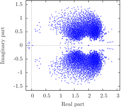 |
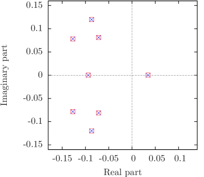 |
| (a) | (b) |
Exploiting the complex conjugate structure of the eigenvalue spectrum, however, an efficient algorithm for the determination of the sign of the fermion determinant can be constructed. The underlying observation is that the sign of is directly given by the number of eigenvalues with zero imaginary part being situated in the half plane with negative real part according to
| (3.144) |
These eigenvalues can actually be computed in practice with the help of an implementation of the Arnoldi-algorithm [164], which allows to find approximations for a specified number of eigenvalues of a non-hermitian matrix, such as the fermion matrix , with a specified accuracy. For our purpose, the most important feature of the latter algorithm is that the aforementioned eigenvalues can be calculated ordered by their real part, for instance, in ascending order. By virtue of the Arnoldi-algorithm it is therefore feasible in practice to compute only those eigenvalues of the fermion matrix that exhibit a negative real part, allowing to determine the value of , and thus the sign of according to Eq. (3.144), without having to evaluate the full eigenvalue spectrum.
For clarification it is remarked that the described approach relies on the number of eigenvalues exhibiting a negative real part to be sufficiently small. Otherwise the determination of these eigenvalues would again become unfeasible from a practical point of view. For such cases, there also exist some more advanced techniques [165, 166], which derive the sign of from a transformed operator for some polynomial , keeping the relevant eigenvalues, i.e. those with zero imaginary part, invariant but rotating those with non-zero imaginary part into the positive half-plane. The idea of that approach would be to end up with a reduced number of eigenvalues with negative real part, thus lowering the numerical effort for their determination. However, it was found that only a small fraction of the eigenvalues being of order has a negative real-part such that the simpler approach already solves the problem satisfactorily in our case. It will therefore be the method of choice in the following.
In the analysis of the generated field configurations the sign of the determinant has originally been monitored and included into the calculation of all observables as required to guarantee the correctness of the applied algorithm. However, even after the analysis of thousands of configurations produced in actual Monte-Carlo calculations not a single negative sign has been observed for those parameter settings which are of physical interest in this study. At some point the further analysis of the sign of the fermion determinant has therefore been stopped in order to save computational resources for more promising calculations.
3.6.2 General case
For unequal Yukawa coupling constants, i.e. , the relation for the operator in Eq. (3.139) is violated, thus invalidating the proof of the complex conjugate eigenvalue spectrum of given in the preceding section. In fact, the spectrum of the fermion matrix is not complex conjugate for unequal Yukawa coupling constants as demonstrated in Fig. 3.2, where an example of the full eigenvalue spectrum is presented for a randomly chosen field . It was also numerically confirmed that the corresponding fermion determinant is indeed not real.
However, in Fig. 3.2 one can still observe a complex conjugate main structure induced by the circular and complex conjugate spectrum of the free overlap operator. The eigenvalues deviate around this base structure according to the strength of the Yukawa coupling constants. For sufficiently small coupling parameters , one would therefore expect the distribution of the phase to be dominated by a peak around its center value at zero. In the limit one would moreover assume the width of this distribution to vanish. An example of the distribution of is presented in Fig. 3.3a. Here, the phase of the fermion determinant has been determined numerically for several thousand randomly chosen field configurations. The choice of the Yukawa coupling parameters corresponds to the setting that will later be used for the physically motivated evaluations of the model. One sees that even for this not very small coupling strength the phase of does not wildly oscillate over the full interval but is already clearly restrained.
Besides the complex conjugate base structure of the fermion matrix there is an additional observation that helps to explain the small fluctuation of the phase . In fact the spectrum of is still complex conjugate provided that the underlying field is identical to its time-reversal . For clarification let be the time-reversal operator, acting on the space of pseudo fermion fields, according to
| (3.145) |
One then finds
| (3.146) |
which can be used to establish the announced result. For that purpose let be an eigenvalue of . Employing the above result one can show that the complex conjugate value is also an eigenvalue of according to
| (3.147) | |||||
where the time-reversed field is given as
| (3.148) |
and has been assumed. The spectrum of the fermion matrix is therefore complex conjugate also in the general case with provided that the underlying field configuration is invariant under time reflection, i.e. , or equivalently, .
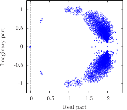 |
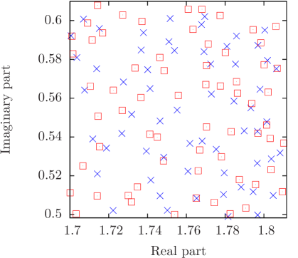 |
| (a) | (b) |
For clarification it is remarked that the correct derivation of the result in Eq. (3.147) actually requires to pay special attention to the zero modes of the operator . This can be worked in detail by employing the projection operator in Eq. (4.52) and exploiting the relation in Eq. (4.2.1), which will be introduced and applied to the considered Higgs-Yukawa model in section 4.2.1. The result in Eq. (3.147) is, however, unaltered by this more careful calculation.
From the aforementioned result one may conjecture that the constraint on the phase observed in Fig. 3.3a should become even more pronounced in the background of the physically relevant field configurations, which exhibit a non-vanishing vacuum expectation value . The reasoning is that in this case the amplitude of the zero momentum mode of the scalar field , which is invariant under time reflection, is the most dominant mode. An example of this scenario is shown in Fig. 3.3b, where the distribution of is presented as observed in a Monte-Carlo calculation performed in the broken phase with a model parameter setup which is typical for the later lattice investigations. One clearly observes the complex phase of the respective fermion matrices to be much stronger constraint than for the case of the previously discussed random configurations.
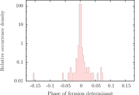 |
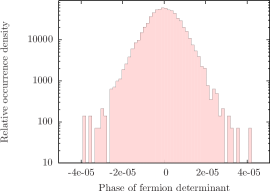 |
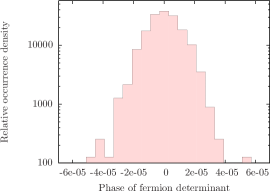 |
| (a) | (b) | (c) |
The presented results on the distribution of as displayed in Fig. 3.3a and Fig. 3.3b have been obtained on very small -lattices, where the direct computations of all eigenvalues of were easily feasible. The vital question is how the behaviour of the complex phase changes on larger lattice volumes. To obtain an indication on how the lattice volume might influence the distribution of an additional Monte-Carlo calculation has been performed on a larger -lattice, however with identical Yukawa coupling constants and tuned hopping parameter aiming at the reproduction of the previously observed lattice result on the vacuum expectation value . The distribution of the complex phase of the fermion determinant resulting from this larger volume computation is presented in Fig. 3.3c. The main observation is that the increased lattice volume, which was amplified here by a factor of approximately compared to the -lattice, does not seem to have a pronounced impact on the distribution of , which is a rather encouraging finding.
However, it should be stressed at this point that there is no obvious way of how the phase of the fermion determinant can be accounted for in a practical numerical calculation, once the lattice volume becomes too large for the direct computation of the full determinant. The phase of will therefore be neglected in our simulation algorithm in the case of unequal Yukawa coupling constants.
Consequently, all results obtained for are effected by an unknown systematic uncertainty given by the constraint of . The major analysis of the considered model will therefore be performed in the degenerate case with where the simulation algorithm is exact. From the presented indications one may, however, conjecture that the aforementioned systematic uncertainty of the results obtained for unequal Yukawa coupling constants in the broken phase should be on an acceptable level compared to the statistical uncertainties also on larger lattice volumes.
Chapter 4 The phase diagram in the large -limit
In this chapter the phase structure of the given lattice Higgs-Yukawa model will be discussed. The order parameters being considered in the following to distinguish the different phases are the vacuum expectation value of the rotated field as defined in Eq. (3.56) and its staggered counterpart, the staggered vev , which is specified below. For the purpose of this chapter, however, an equivalent definition for the vev is used, which expresses and the staggered vev in terms of the so-called magnetization and the staggered magnetization according to
| and | (4.1) |
where the latter observables are defined as
| and | (4.2) |
with denoting the so-called staggered momentum .
For clarification it is remarked that there actually is no direct physical interpretation assigned to the staggered vev in the context of this work, though the latter quantity can indeed be physically relevant in the framework of other studies, for instance for the investigation of anti-ferromagnetism in solid state physics. In the lattice approach employed here to examine the pure Higgs-Yukawa sector of the Standard Model in the spontaneously broken phase, however, the staggered vev has to vanish in physical units111This is a stronger requirement than, for instance, for the vev , which only has to vanish in dimensionless lattice units in the continuum limit. in any attempt of constructing a physically meaningful continuum limit. The consideration of both observables nevertheless has an interesting motivation beyond the obvious fact that it yields a more complete understanding of the investigated model. It directly marks all those regions in parameter space as physically uninteresting for the purpose of this study, where the model exhibits a non-vanishing staggered vev . Furthermore, it serves as a probe for the structure of the ground state of the model, yielding additional information needed for the determination whether a phase, that exhibits a vanishing vev , actually is a symmetric phase, which would require the respective ground state to be . For instance, a staggered-broken phase (, ) would mistakenly be identified as a symmetric phase, if the staggered vev was not taken into account.
For the eventual aim of determining the Higgs boson mass bounds the identification of the second order phase transition surfaces separating the broken phases with , and the symmetric phases is an important prerequisite, since these regions directly constitute the areas in bare parameter space where the eventual calculations of physical interest have to be performed, as discussed in section 2.3.3. In all generality, the phase structure of the investigated model cannot be given in analytical form. It can, however, be investigated in certain limits of the model.
Following the ideas of LABEL:Hasenfratz:1992xs different approaches will be presented in the subsequent sections that allow for the determination of the phase structure in the limit of an infinite number of fermion generations . These calculations are performed in the mass degenerate case with equal top and bottom Yukawa coupling parameters . The reasoning is that almost all later lattice calculations will be performed in that scenario due to the uncertainties222Additional concerns related to the non-degenerate case will be discussed in section 6.4.2. otherwise arising from the complex phase of the fermion determinant as discussed in section 3.6.2.
At the end of each section the analytical results in the respective approximation are compared to corresponding direct Monte-Carlo calculations. These numerical data have been produced by the HMC-algorithm introduced in section 3.5, which by construction is applicable for even values of only.
4.1 Small Yukawa and quartic coupling constants
In this section the phase structure of the considered lattice Higgs-Yukawa model will be investigated in the large -limit for small values of the quartic coupling parameter and the degenerate Yukawa coupling constant . More precisely, the limit is studied with the coupling constants scaling according to
| (4.3) |
where the parameters , , and are held constant in that limit procedure.
4.1.1 Analytical calculations
The starting point for the subsequent analytical calculation of the phase structure is the observation that in the considered limit a factor of can be factorized out of the action given in Eq. (3.45) according to
| (4.4) |
where the rescaled bosonic and fermionic actions and are given as
| (4.5) |
and333According to the fermion determinant can also be written entirely in terms of the rescaled parameters and fields, which will later explicitly be done.
| (4.6) |
respectively. In the limit the functional integration over all field configurations in Eq. (3.44) then reduces to a sum over all absolute minima444With some abuse of notation the notion ’minimum’ is used here and in the following also as a synonym for the more precise formulation ’location of the minimum’. of . The expectation values of the rescaled order parameters and are then directly obtainable from the knowledge of these ground states.
To make a determination of these states feasible in practice we consider here the restricted ansatz
| (4.7) |
for the ground states of , taking only a constant and a staggered mode into account, where the real numbers , and the unit vectors , specify the amplitudes and orientations, respectively, of the constant and staggered momentum modes. This restriction is reasonable, since we are eventually interested in locating those phases, in which the ground states are translational invariant. The staggered mode is also included within this ansatz to allow for the determination of , which is desirable for the aforementioned reasons. For a given ground state parametrized in terms of Eq. (4.7) the corresponding contribution to the rescaled order parameters and would then be given as and , respectively.
It is, however, not guaranteed that the true ground states of the action can actually be parametrized in terms of Eq. (4.7). In fact, we will later observe phases derived by the given ansatz, that simultaneously exhibit a non-vanishing vev and a non-vanishing staggered vev , which can be understood as an indication for the true ground state structure being more complex than assumed in this simple approach. The restriction of the consideration to the ansatz in Eq. (4.7) has thus to be understood as a working hypothesis only. The obtained analytical results on the phase structure are therefore later explicitly confronted with corresponding numerical data obtained in direct Monte-Carlo calculations.
So far, the given conceptual background of the large -analysis is rather crude. A deeper understanding can be achieved by considering the constraint effective potential [168, 72] which is defined as
| (4.8) |
up to some constant independent of the arguments and . Here the original definition in LABEL:Fukuda:1974ey,O'Raifeartaigh:1986hi has been extended to depend not only on the amplitudes of the constant momentum modes but also on the amplitudes of the staggered modes. In the above definition the expression denotes the scalar field in momentum space according to
| (4.9) |
With the help of this constraint effective potential the expectation value of any observable depending solely on the constant and the staggered modes of the scalar field , such as the magnetizations and defined in Eq. (4.2), can then be written as
| (4.10) |
where the latter effective integral is given as
| (4.11) |
The constraint effective potential thus has a manifest interpretation. It is directly connected to the probability distribution of the momentum mode amplitudes and according to as observed, for instance, in a corresponding Markov process. For sufficiently large lattice volumes the expectation value of the considered observable can thus directly be obtained from the minima of the constraint effective potential. This is clear from the integral representation of the latter quantity in Eq. (4.10), which is obviously dominated by the minima of for sufficiently large lattice volumes due to the explicit appearance of the volume555The volume appears explicitly in Eq. (4.11) according to the actions and underlying the definition of being extensive quantities, scaling proportional to the lattice volume . in the weight factor in Eq. (4.11).
It is further remarked that the finite volume constraint effective potential is not a convex function in general [72]. In particular, it can, for instance, exhibit the famous Mexican hat structure with a non-zero minimum, being unique apart from the trivial degeneracy induced by the symmetries of the model, signaling then the situation of spontaneous symmetry breaking. This is illustrated in Fig. 4.1a, sketching a finite volume example of the less general potential , defined analogously to Eq. (4.8) including, however, also the staggered mode in the bosonic integration, as originally defined in LABEL:O'Raifeartaigh:1986hi.
This is in contrast to the situation of the infinite volume, where the constraint effective potential can be proven to be always convex [72]. In infinite volume the latter constraint effective potential can therefore never assume the aforementioned Mexican hat structure, or any other non-convex form. In a model parameter setup, where spontaneous symmetry breaking occurs, the infinite volume constraint effective potential would then take the form of a convex hull, for instance, of the Mexican hat potential which, however, does not possess a unique minimum even if one factors out the aforementioned degeneracy induced by the symmetries of the model. This observation can be generalized to the statement that the infinite volume constraint effective potential, which has to be convex, becomes exactly flat at its minima and possesses a manifold of degenerate minima in the latter sense, if the model exhibits spontaneous symmetry breaking. A corresponding example is sketched in Fig. 4.1c.
For the case of a finite volume we shall always assume the constraint effective potential to possess a single, unique minimum in the following, where the notion of a ’single’ minimum is used here with some abuse of notation to distinguish the case illustrated in Fig. 4.1a from the one in Fig. 4.1c. In fact, the minimum in the former case is also degenerate according to the symmetries of the model. This shall, however, implicitly be understood in the following when using the terms ’single minimum’ or ’unique minimum’ versus ’degenerate minimum’. This is a reasonable notation, since we will only be interested in observables being invariant under the latter symmetries.
Concerning the infinite volume, however, the alert reader might wonder, whether the statement, that the integral in Eq. (4.11) is dominated by the minimum of the constraint effective potential, does actually make sense in the scenario of spontaneous symmetry breaking, since the infinite volume constraint effective potential then possesses a manifold of degenerate minima as illustrated in Fig. 4.1c. The key observation in this respect is the following. For any finite volume, the constraint effective potential does not need to be convex. In particular, it can then exhibit, for instance, the Mexican hat structure with a single, non-zero minimum. As the volume increases the constraint effective potential finally becomes convex. In the sketched example of the Mexican hat potential, the bump in the center vanishes in the thermodynamic limit, as illustrated in Fig. 4.1b. The crucial question is, how fast it decreases. Explicit lattice calculations [72] of the constraint effective potential performed in the four-dimensional pure -theory find that the latter decline is much slower than . The weight factor appearing in Eq. (4.11), however, explicitly contains a factor of the volume , such that the effect of the integral in Eq. (4.11) being dominated by the non-degenerate minimum of the finite volume constraint effective potential becomes in fact more pronounced as the finite volume is increased, although the constraint effective potential itself finally becomes convex. Conceptually, it is therefore not the infinite volume limit of the constraint effective potential itself, that is actually of interest, but instead the infinite volume limit of the position of its finite volume minimum, when studying the thermodynamic limit of the underlying model.
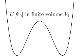 |
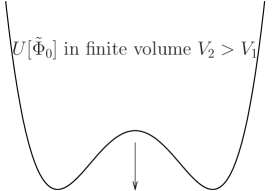 |
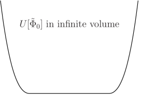 |
| (a) | (b) | (c) |
It is remarked that the above considerations referred to the exact constraint potential. In the following, however, we will calculate the constraint effective potential only to a finite order in perturbation theory, in fact to tree-level in this chapter and to one-loop order, at least with respect to the purely bosonic contributions, in section 6.3. The computed results on the constraint effective potential will therefore not be convex even in the infinite volume limit. From a practical point of view the above subtleties of taking the infinite volume limit of the potential itself or rather of its minimum will therefore not play a role in the following. In this respect we will occasionally speak about ’the minimum’ of the constraint effective in infinite volume, having then always in mind what has been said here.
It is further remarked that the constraint effective potential in finite volume is not the same object as the effective potential [39, 169] , being defined by means of a Legendre transformation of the generating functional . It is only the thermodynamic limit that drives [72] the constraint effective potential to converge to the effective potential . In contrast to , the effective potential is always a convex function, also in finite volume. In fact, one can show [72] that is the convex hull of . For clarification it is, however, pointed out that the effective potential will not be considered in the present work.
For the here intended investigation of the phase structure of the underlying Higgs-Yukawa model, the basic idea is to determine the absolute minimum of the constraint effective potential with respect to and , which would then directly yield the considered order parameters and at least for sufficiently large lattice volumes . This can be done, for instance, in the large -limit, where the analytical calculation of the constraint effective potential can greatly be simplified. For that purpose we equivalently rewrite the definition of the constraint effective potential in Eq. (4.8) in terms of a purely Gaussian contribution , a solely bosonic tree-level part , and the remaining, interacting contribution according to
| (4.12) |
where has been defined in Eq. (4.7) and the expressions and have been treated synonymously, implicitly assuming the obvious mappings here and in the following.
For the sake of simplicity, we restrict the subsequent considerations to the case of equal orientations, i.e. . In that scenario the so far unspecified expressions for the purely Gaussian contribution and the interacting contribution can be given as
| (4.13) |
and666Appropriate modulo operations are implicit in Eq. (4.1.1) to guarantee all sums and differences of lattice momenta to be contained in .
In the given setup the constraint effective potential can now formally be expanded in terms of a diagrammatic series, each diagram of which having assigned a certain inverse power of [170]. This is achieved by expanding the interacting contribution into a power series and performing the resulting Gaussian integrations over the bosonic modes , and over the fermion fields , . Examples for such diagrams are presented in Fig. 4.2 together with their respective weight in inverse powers of . Basically, the idea is that due to the considered scaling given in Eq. (4.3) each -vertex carries a factor of , while every -vertex has a factor assigned. Furthermore, the amplitudes of the momentum modes with or scale proportional to according to the assumed ground state structure as discussed at the beginning of this section, while the propagators of all other momenta are of order , which formally follows from the given form of the purely Gaussian contribution . A further remark on the latter statement follows below.

In the large -limit with the coupling constants scaling according to Eq. (4.3) one then directly finds
| (4.15) | |||||
| (4.16) |
up to some constant factor777Here and in the following ’constant’ means independent of , , and . 888 does not depend on the orientation as will later be seen. provided that at least one of the two variables is non-zero and that the exponents of the Gaussian factors in the aforementioned Gaussian integrations over the bosonic modes , are positive, which is guaranteed for all values of and , provided that
| (4.17) |
For the considered purpose of determining the phase structure of the Higgs-Yukawa model in the limit one is therefore left with the problem of finding the absolute minimum of with respect to , thus recovering the identical approach already derived from the simple consideration at the beginning of this section.
It is, however, remarked here that the given expansion is only valid if the true ground state of the system actually has the form of Eq. (4.7), which has to be assumed. The reason is that one needs the propagators in the aforementioned diagrammatic expansion to be of order and not , for instance, to derive the above result. In this respect one has not gained additional information as compared to the very simple consideration at the beginning of this section. Given a scenario with a ground state in the form of Eq. (4.7), however, one has learned that the the correction to in the large -limit is of order , which follows by working out the combinatorically possible diagrams arising from the expansion of as systematically discussed in LABEL:Coleman:1988zu. In contrast to the aforementioned earlier consideration the lastly discussed approach based on the effective potential moreover opens the possibility of determining these corrections in powers of . This idea will be picked up again in section 6.3.2, where corrections to will actually be calculated, though in a different context than the large -analysis.
Here, however, we continue with the consideration of the limit . As already pointed out before we have restricted the evaluation of the effective potential to the case of equal orientations . In that setup the purely bosonic part of becomes
| (4.18) |
The remaining calculation of the determinant of the fermion matrix can also be performed analytically due to the simple structure of given in Eq. (4.7). In this approach the fermion matrix in momentum space999With some abuse of notation no new symbol has been introduced for the momentum space representation of and other operators. has a diagonal-plus-subdiagonal-block-structure. In terms of the spinor basis given in Eq. (3.7-3.8) it can be represented as
where the diagonal part is caused by the zero momentum mode of the scalar field , while the sub-diagonal contribution is created by the staggered mode. In Eq. (4.1.1) this is expressed by denoting the shifted momenta , where adequate modulo-operations are implicit to guarantee . The matrices , , , and are -matrices with the indices and denote the spinor basis transformation matrix
| (4.20) |
the Dirac matrix
| (4.21) |
the vertex structure matrix
| (4.22) |
and the Yukawa coupling matrix
in the spinor basis as introduced in Eq. (3.7). Due to this diagonal-subdiagonal-block-structure the determinant in Eq. (4.16) can thus be factorized by merging the four blocks, which correspond to the momentum indices , , , and . Up to some constant terms, which are independent of , one can thus rewrite the effective potential as
| (4.24) |
where the restriction has been introduced to prevent the double counting that would occur if one would perform the product over all after having merged the blocks. Here denotes these merged, momentum dependent matrices given by
| (4.25) |
with
| (4.26) | |||||
| (4.27) | |||||
| (4.28) | |||||
| (4.29) |
The expression in Eq. (4.24) can be written more compactly, taking the fact into account that the involved matrices are diagonal with respect to the index due to Eq. (4.21), Eq. (4.1.1) and
| (4.30) |
Since one easily finds that the determinant in Eq. (4.24) is invariant under the permutation , one can extend the product in that equation, which is performed only over one half of the whole momentum space, again to the full momentum space by factorizing out the identity . One then obtains for the effective potential
| (4.31) |
with the definitions
| (4.32) |
and . Ordering the indices according to the latter four matrices are explicitly given by
| (4.37) | |||||
| (4.43) |
where the abbreviation was used. The remaining matrices and are obtained from , by interchanging and . Using some algebraic manipulation package, the determinant of the matrix in Eq. (4.31) can be computed leading to the final expression for the effective potential
| (4.45) | |||||
The resulting phase structure in the large -limit can now be obtained by minimizing the effective potential with respect to and . This is done here in the infinite volume limit, where the sum over all allowed momenta in Eq. (4.45) becomes a four-dimensional momentum integral over continuous momenta according to
| (4.46) |
which was evaluated with the aid of some numeric analysis software [126].
The resulting phase structure is presented in Fig. 4.3 for the selected values
and . Here, four different phases do emerge
which are labeled in analogy to the terminology of magnetism in solid state physics. These are
(I)
a symmetric phase (SYM): ,
(II)
a broken ferromagnetic phase (FM): ,
(III)
a staggered-broken anti-ferromagnetic phase (AFM): ,
(IV)
and a broken/staggered-broken ferrimagnetic phase (FI): ,
where , denote the location of the absolute minimum of the effective potential according to
.
In both cases, i.e. and , one finds a symmetric phase approximately centered around at sufficiently small values of the Yukawa coupling constant . This is what one would have expected, since the model becomes the pure -theory in the limit . From the same consideration the accompanying phase transitions at small values of the Yukawa coupling constant can also be assumed to be of second order. This is indeed the case here as can be verified by the results presented in Fig. 4.4. In that plots the dependence of , , and thus of the order parameters and , on the hopping parameter is shown to be continuous at sufficiently small values of .
With increasing values of the Yukawa coupling constant the symmetric phase bends downwards to negative values of the hopping parameter , unless it either hits a first order phase transition to an anti-ferromagnetic phase (black line in Fig. 4.3), which is the case for , or it eventually goes over into two FM-FI and FI-AFM second order phase transitions, as observed for the selected value . The order of these phase transitions can again be determined by considering the dependence of , on , which is presented in Fig. 4.5.
It is remarked that the results on the -dependence of , have only been depicted here for the setting and not for , since the latter plots would not provide qualitatively new information.
However, though the obtained expression in Eq. (4.45) seems to be applicable for any value of it actually only yields a meaningful result for the effective potential in the large -limit if the precondition in Eq. (4.17) is fulfilled. This induces an absolute bound for the validity of the presented calculation of . Moreover, the obtained phase diagrams can only be trusted for . Whether the obtained results beyond that threshold are still in agreement with the true phase structure of the model has to be checked explicitly, for instance, by direct Monte-Carlo calculations.
It is therefore an open question at this point, whether the rather surprising appearance of the ferrimagnetic phase (FI) observed in both presented scenarios, i.e. for and , even deeply inside the anti-ferromagnetic phase region, is actually present in an exact evaluation of the phase structure. This question will explicitly be investigated in the subsequent section.
4.1.2 Comparison with direct Monte-Carlo calculations
Now the predicted phase structure shall be confronted with the results of direct Monte-Carlo calculations performed by means of the HMC-algorithm introduced in section 3.5. To determine the exact location of the phase transition, the susceptibilities , of the magnetizations defined as
| (4.47) |
are fitted as functions of the hopping parameter to the – partly phenomenologically motivated – ansatz [171]
| (4.48) |
where , , and are the fitting parameters for the magnetic susceptibility and the staggered susceptibility , respectively, while and denote the critical exponents101010The critical exponents , , and are defined here through the infinite volume behaviour of the correlation length , the susceptibility , and the magnetization at the phase transition according to , , and , where is assumed to be positive in the latter case. of the pure -theory. Neglecting all subleading, logarithmic contributions one can infer111111The scaling behaviour of the correlation length, i.e. the inverse mass, and the vacuum expectation value at the phase transition, which has been derived in LABEL:Luscher:1988uq, is explicitly given in Eq. (7.2) and Eq. (7.3). from LABEL:Luscher:1988uq that the critical exponents and of the four-dimensional, four-component pure -theory are given as to lowest order. Exploiting the hyperscaling relations provided in LABEL:Kleinert:2001zu the so far unspecified parameter can then be derived from the values of and yielding the result .
For clarification it is remarked that the notation actually refers to two parameters, namely for and in the other case, such that the resulting curve is not necessarily symmetric. An analogous statement holds for . The SYM-FM and SYM-AFM phase transition points are then given by the critical hopping parameters , where the magnetic and staggered susceptibilities develop their respective maximum.
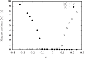 |
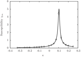 |
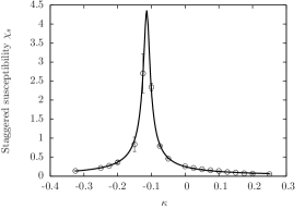 |
| (a) | (b) | (c) |
A typical example for such a determination of the phase transition points is presented in Fig. 4.6 for a rather small value of the Yukawa coupling constant. The average magnetizations and as well as the corresponding susceptibilities are shown as a function of . The vanishing of the average magnetization and staggered magnetization is clearly observed when the symmetric phase is entered, except for some small finite volume effects. Associated to these phase transitions are peaks in the susceptibilities as expected, which can very well be described by the fit ansatz in Eq. (4.48). It is remarked that this ansatz, though not unique, provides a very good description of the numerically obtained data leading to a reliable determination of the critical hopping parameters at least for the here considered small values of the Yukawa and quartic coupling constants.
Using the strategy just described the values of and have been computed for various Yukawa coupling constants , while holding the quartic coupling parameter at the constant value . In Fig. 4.7 the numerical results on the phase structure are presented as obtained by direct Monte-Carlo calculations on a - and a -lattice with . These numerical findings are compared to the phase structure which was analytically determined in the infinite volume and infinite -limit. On a qualitative level the analytical and the numerical results are in very good agreement. As expected, a symmetric (SYM), a ferromagnetic (FM) and an anti-ferromagnetic (AFM) phase can be observed in the obtained lattice data. Moreover, the numerically determined symmetric phase bends strongly towards smaller values of the critical hopping parameter, when the Yukawa coupling constant is increased, as predicted.
It is remarked that the simulations become much more demanding when entering the anti-ferromagnetic phase, due to an increasingly bad condition number of the fermion matrix . Within the anti-ferromagnetic phase numerical results are therefore only presented on rather small -lattices here.
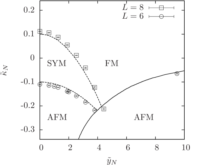
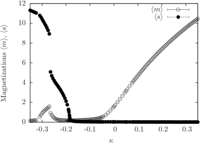 |
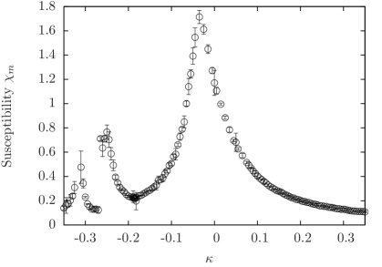 |
| (a) | (b) |
Besides these three phases the analytical calculation in section 4.1.1 has also predicted a fourth, somewhat peculiar phase, where both, the average magnetization as well as its staggered counterpart , are simultaneously non-zero. This so-called ferrimagnetic (FI) phase was found to appear at intermediate values of the Yukawa coupling constant deeply inside the anti-ferromagnetic phase. In Fig. 4.8 evidence for the existence of this ferrimagnetic phase is provided. Its location within the phase diagram is in good agreement with the analytical prediction. However, the ferrimagnetic phase is not within the prime interest of this study and is therefore not further investigated here.
Concerning the order of the encountered phase transitions one can conjecture that the SYM-FM as well as the SYM-AFM phase transition are of second order according to the continuous dependence of and on the hopping parameter as seen for instance in Fig. 4.8a. This is in full agreement with the corresponding predictions based on the analytical calculations in section 4.1.1. Contrarily, the direct FM-AFM phase transition occurring at intermediate values of the Yukawa coupling constant was predicted to be of first order. To clarify this an example of such a phase transition as obtained from the numerical calculations is presented in Fig. 4.9. In panel (a) one can clearly observe an abrupt jump in the dependence of and on the hopping parameter indicating a discontinuous phase transition. Furthermore, an example of a tunneling event between two distinct ground states as observed in a Monte-Carlo run performed close to the critical value is presented in subfigures (b) and (c), serving as another strong indication for the first order nature of the considered phase transition. However, the order of this phase transition is not studied by more elaborate methods here, since this is not in the main interest of the present study.
Qualitatively, all presented findings are in very good agreement with the analytical large calculations in section 4.1.1. On a quantitative level, however, the encountered deviations in Fig. 4.7 need to be further addressed. These deviations can be ascribed to finite volume effects as well as finite corrections.
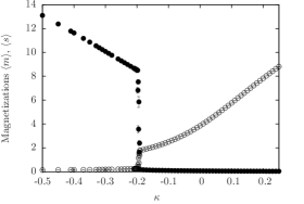 |
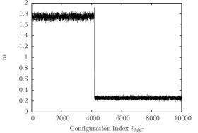 |
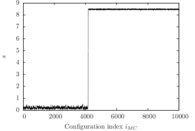 |
| (a) | (b) | (c) |
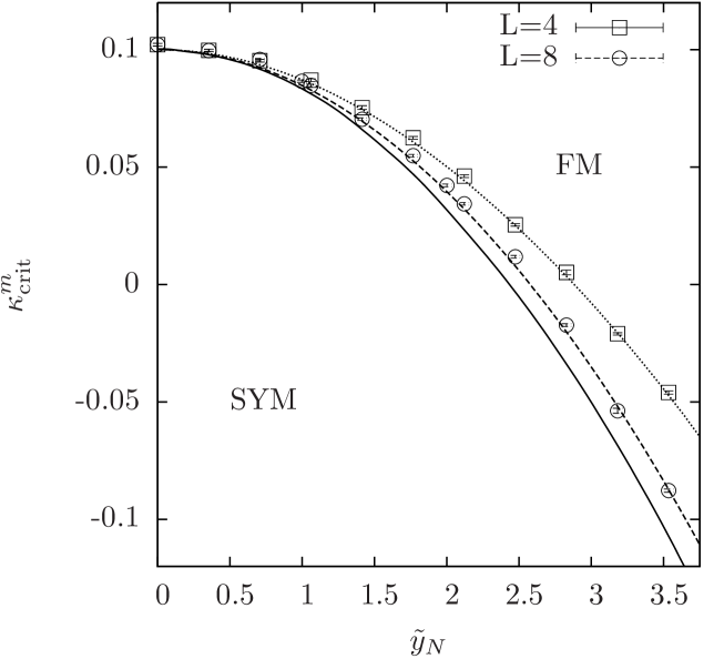
The strength of the finite volume effects is illustrated in Fig. 4.10, where the critical hopping parameter dividing the ferromagnetic from the symmetric phase is presented for several selected values of the Yukawa coupling constant. These results have been obtained from numerical calculations performed with on a -lattice (open squares), and on an -lattice (open circles). The rather large number has been chosen here in order to demonstrate the finite volume dependence isolated from the -dependence. One can clearly observe that the phase transition line is strongly shifted towards smaller values of the hopping parameter when the lattice size is increased.
This effect can also be anticipated by the analytical determination of the phase transition line, when one imposes finite lattice sizes for the calculation of the effective potential in the large approximation. In Fig. 4.10 the resulting analytical finite volume, large predictions for the phase transition lines are depicted by the dotted, dashed, and solid curves representing the cases of the -lattice, the -lattice, and the infinite volume limit, respectively. Comparing these results with the numerically obtained data for the critical hopping parameters one sees that the aforementioned curves describe the numerical findings very well. One can also observe the convergence of the numerically obtained critical hopping parameters to the analytically predicted infinite volume phase transition line as the lattice size increases.
Concerning the analytical large -calculation of the phase transition points on a finite lattice volume, it is remarked that the fermion determinant becomes identical to zero in finite volume, if both parameters and , underlying the considered ansatz for the sought-after ground state, vanish exactly. The analytical finite volume calculation will thus never predict a phase where and are simultaneously identical to zero. In case of a finite lattice volume the phase transition points to the symmetric phase can therefore not be determined by simply searching for that value of the hopping parameter , where the average magnetizations predicted by the analytical calculation become exactly zero. This difficulty does not occur in case of an infinite lattice volume, since the zero modes of then form a set of only zero measure and the integral entering the effective potential in Eq. (4.45) can be shown to yield a finite value even at , such that there actually is a symmetric phase in the sense of the ground state being in the infinite volume limit.
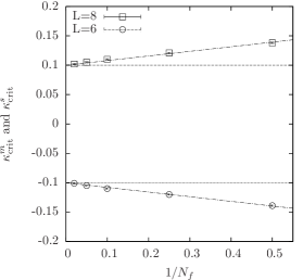 |
 |
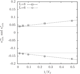 |
| (a) | (b) | (c) |
For the purpose of finding the critical hopping parameters also in the finite volume scenario a different approach is therefore needed. Here has been determined by finding that value of , where the absolute minimum of the effective potential becomes flattest, i.e. where the second derivative of the effective potential at the location of its minimum with respect to and , respectively, becomes minimal. Since the scalar field oscillates the stronger around this minimum the smaller its second derivative is, this approach corresponds to finding the phase transition point by searching for the maximum of the susceptibility.
Finally, the -dependence of the numerically obtained critical hopping parameters and is shown in Fig. 4.11 for several selected values of the Yukawa coupling constant. One clearly sees that for increasing the numerical results converge very well to the analytical finite volume, large predictions, as expected. It is interesting to note that the leading order contribution of the finite corrections, which is of order as discussed in section 4.1.1, seems to be the only practically relevant correction here, even at the smallest, with the HMC-algorithm accessible value . This can be seen in Fig. 4.11 by fitting the observed deviations between the large predictions and the numerical finite results with the fit ansatz with being the only free parameter. Furthermore, one observes that the critical hopping parameter is shifted towards larger values with decreasing while is shifted towards smaller values.
From the presented numerical results one can conclude that the structure of the phase diagram of the considered Higgs-Yukawa model at small values of the quartic and Yukawa coupling constant is very well described on a qualitative level by the results of the analytical large calculation presented in section 4.1.1. It also gives a very good understanding of the encountered finite volume effects.
4.2 Large Yukawa and small quartic coupling constants
In this section the phase diagram of the considered Higgs-Yukawa model will be studied in the regime of large values of the Yukawa coupling constant and small values of the quartic coupling parameter . This is done by considering the limit of a large number of degenerate fermion generations while scaling the coupling parameters according to
| (4.49) |
where the quantities , , and are held constant in that limit procedure.
4.2.1 Analytical calculations
The starting point of the analytical investigation of this large -limit is again the constraint effective potential given in Eq. (4.8). Here, however, we will use the equivalent definition
| (4.50) |
based on the effective fermion action given in Eq. (3.46).
The intended analytical calculation of the constraint effective potential can then be performed in three steps. Firstly, the effective fermion action is expanded in powers of the inverse Yukawa coupling constant . Taking only the first non-vanishing contribution of this power series into account and performing the large -limit as specified in Eq. (4.49), the model can then be shown to effectively become an -symmetric, non-linear sigma-model up to some finite volume terms. Finally, the phase diagram of the latter sigma-model is determined by investigating the resulting expression for the effective potential in some later specified large approximation, where denotes the number of components of the field , i.e. in our case.
For the investigation of the effective action in finite volume it is crucial to pay special attention to the modes in the unphysical corners of the Brillouin zone given as
| (4.51) |
where the vectors have explicitly been defined in Eq. (3.7). These modes will be referred to in the following as -modes. Given these -modes one can define the corresponding projection operator
| (4.52) |
projecting to the sub-space spanned by . Using this notation it is straightforward to establish the very helpful relation
where and are arbitrary operators defined on the same space as and . Here the expression denotes the determinant of with respect to the sub-space and is the determinant of with respect to the complementary space , where denotes the full set of all modes . Using Eq. (4.2.1) several times one can rewrite the effective action, neglecting constant factors independent of , according to
where the introduction of the underscore through is only intended to make the dependence on the Yukawa coupling constant explicit for the sake of a better readability. Here , , and denote the restrictions of the operators , , and to the sub-space . This restriction is introduced, since it guarantees to be invertible. The operator is then defined by extending the domain of the inverse of again to the full space by inserting the projector according to
| (4.55) |
which is well-defined and finite over the whole space . The last determinant in Eq. (4.2.1) can further be reduced by using the relation
| (4.56) | |||||
and by applying again Eq. (4.2.1) leading then to the compact notation for the effective action
| (4.57) | |||||
Here the abbreviation is defined as the somewhat lengthy expression
| (4.58) |
It is remarked that the latter determinants only give rise to some finite volume effects, since these determinants are only performed over the 120-dimensional sub-space . Their contributions to the effective action do therefore not scale proportional to the volume as the lattice size increases in contrast to all other appearing terms. We will come back to discussing these finite volume effects later. Here, however, we first continue with the evaluation of the last term in Eq. (4.57) by rewriting the corresponding trace as a power series in the inverse coupling constant according to
| (4.59) |
and by eventually cutting off this power series after the first non-vanishing term, which is well-justified for sufficiently large values of . For the purpose of establishing the desired connection to a sigma-model it is most convenient to evaluate these expressions in position space. Then the matrix is block diagonal and explicitly given by
| (4.60) |
where the notation , was used, was defined in Eq. (3.50), and the underscore indicates again a simple rescaling with the factor . In position space the matrix can hence be written as
with as defined in Eq. (4.1.1). The scalars denote the eigenvalues of the anti-hermitian operator corresponding to its eigenvectors and are explicitly given by
| (4.64) |
The result for the trace of the operator is then directly found to be
| (4.65) |
which can be generalized to the trace of the -th power of yielding
| (4.66) |
with being identified with , and with . Here the expression stands for the diagonal matrix
| (4.67) |
The trace appearing in Eq. (4.66) can be further simplified by inserting the identity at some proper places leading then to
| (4.68) |
with given as
| (4.73) | |||||
Here, the relation has been exploited. Due to the insertion of the spinor basis transformation matrices and the sums over the momenta in Eq. (4.66) factorize now according to
| (4.74) | |||||
| (4.75) |
where the momentum sum is a four-dimensional Fourier transform of an anti-symmetric and purely imaginary function, hence yielding real values. With the definition
| (4.76) |
the hermitian -matrix can compactly be written as
| (4.77) |
leading directly to the result that the lowest order contribution of the power series in Eq. (4.59) vanishes according to
| (4.78) |
The first non-vanishing contribution is the second order term, which can be evaluated by explicitly computing the trace, yielding
| (4.79) | |||||
Cutting off the power series in Eq. (4.59) after this first non-vanishing term, which is well justified for sufficiently large values of the Yukawa coupling constant , the effective fermion action can thus be written as
As already pointed out the determinants are taken with respect to the -dimensional space . In contrast to all other terms appearing in the effective action these determinants are not proportional to the volume . They are therefore suppressed as the lattice size goes to infinity. Moreover, the very last term in Eq. (4.2.1) even vanishes on finite lattice sizes when the Yukawa coupling constant becomes sufficiently large. This is in contrast to the determinant being independent of . It is therefore quite instructive to evaluate the latter finite volume contribution in more detail, which can be done at least if one restricts the consideration to the ansatz given in Eq. (4.7) taking only a constant and a staggered mode of the scalar field into account. The neglection of all other modes is not rigorously justified here, but motivated by the fact that in the broken (staggered-broken) phase the constant (staggered) modes yield the most dominant contributions. A crude estimate of the effect of should thus be obtainable from this approach. Taking again only one orientation into account, i.e. , one finds
| (4.81) |
with the abbreviations
| (4.82) |
The resulting asymmetry in and is caused by the fact that the zero modes are not included in the sub-space . The effect of the latter terms and especially the resulting asymmetry in and is clearly observed in corresponding Monte-Carlo simulations on small lattices and large values of the Yukawa coupling constant as discussed in the subsequent section. Moreover, the result in Eq. (4.81) would also hinder the expectation value from vanishing, thus obscuring the potential existence of symmetric phases at large values of on small lattices. However, as the lattice volume increases these finite volume effects eventually disappear relative too the contributions given in the upper row of Eq. (4.2.1). In the following the -terms will therefore be neglected, which is well justified on sufficiently large lattice volumes.
To establish the announced connection to a sigma-model we now consider the large -limit where the coupling constants scale according to Eq. (4.49). With some implicit substitution of the integration variables the effective potential in Eq. (4.50) can then be written as
| (4.83) |
up to some constant terms independent of the variables , and the orientations , where the actions and are given as
| (4.84) | |||||
| (4.85) |
From this result one finds that the effective potential is dominated by the action in the large -limit which, however, is completely independent of the hopping parameter . Taking only this contribution into account would thus not allow to study the phase transition with respect to . For that purpose the suppressed contribution also needs to be accounted for, which can be done in the large -limit according to
| (4.86) |
where again constant terms have been neglected and is given as
| (4.87) |
according to the substitution and denoting the Fourier transform of defined analogously to Eq. (4.9). Here the dominant contribution has enforced and equivalently for all space-time points , where the amplitude is given by the determination equation
| (4.88) |
while reflects the sub-leading dynamics induced by . With this fixation of the scalar field amplitude the model in Eq. (4.2.1) effectively becomes a non-local, four-dimensional, non-linear sigma-model in the infinite volume and large -limit according to
| (4.89) |
with the effective, non-local coupling matrix
| (4.90) |
Here the notion ’non-local’ simply refers to the fact, that the field at a given lattice site is coupled to at any other site of the lattice. This leaves nevertheless open the possibility that the interaction is still local in a field theoretical sense with exponentially decaying coupling strength [143]. This question was, however, not investigated in detail, since the eventual interest of this study focuses on the small Yukawa coupling regime.
It is remarked that the outcome in Eq. (4.90) reproduces the result which was found for a Higgs-Yukawa model based on Wilson fermions [167] with the only difference that the coupling matrix in that case consisted solely of nearest-neighbour couplings.
It is further remarked that the extension of this analysis to the case, where the quartic coupling constant is not small, i.e. , is straightforward. In that case the quartic coupling term in Eq. (4.85) would not scale proportional to but proportional to instead, thus making the quartic coupling term the most dominant contribution in the large -limit. One would then still end up with a -model based on the same coupling matrix as given in Eq. (4.90), but with the difference that the determination equation for in Eq. (4.88) would reduce to the trivial condition . However, this part of the phase diagram is not in the main interest of this study and is thus not further investigated here.
The desired phase structure of the considered Higgs-Yukawa model can now be obtained by minimizing the effective potential of the associated -model with respect to and . However, the direct computation of is hindered by the constraint of the integration variables in Eq. (4.87), which is a general obstacle for investigating -models. The crucial step towards the evaluation of is thus the removal of the constraint . For that purpose the restriction can be encoded as a -function [173, 174] written in terms of an integration of the term over the newly introduced one-component real scalar field .
In this approach the constraint effective potential of the -model can be written as
| (4.91) |
where constant terms have again been neglected and the action is given as
| (4.92) |
with . Up to this point the choice of is free. For later convenience we set , where is space-time independent. So far, the calculation performed with respect to the sigma model is exact. The first approximation occurs in the following step, where the action is replaced by defined as
| (4.93) |
where and . The consideration was here restricted to the constant mode of , which was found to be justified121212The approach considered in LABEL:Flyvbjerg:1988em differs slightly. There the Gaussian integration over is performed first, explicitly revealing then the resulting effective action to scale proportional to , being thus dominated by the ground states of the remaining fields and in the limit . The -field content of these ground states was then found to be well describable by considering only the constant mode of . in LABEL:Flyvbjerg:1988em for sufficiently large values of , with denoting the number of components of , i.e. in this case. Whether this approximation is justified here will turn out in the subsequent section, where the resulting analytical results will be compared to direct Monte-Carlo calculations. If one accepts this approximation one can write the associated approximation of the effective potential as
| (4.94) |
up to constant terms where the action is obtained from by integrating out the modes , according to
| (4.95) | |||||
which is mathematically well-defined only if was chosen sufficiently large, which will turn out to be the case, at least for the SYM-FM phase transition, after having solved the resulting gap equations. At this point we continue with this formal expression and postpone the discussion of the validity of the performed Gauss integration to the end of this section.
In the latter result the shorthand notations and were used, denoting the constant and staggered modes according to
| (4.96) |
being eigenvectors of the effective coupling matrix . Furthermore, is the determinant restricted to the space , thus neglecting the two latter modes. For convenience, this short-hand notation will also be applied in the following where it is unambiguous.
To evaluate the determinant in Eq. (4.95), the eigenvalues of the effective coupling matrix need to be known. The eigenvectors are simply plane waves with wave vectors and one easily finds the corresponding eigenvalues according to
| (4.97) |
where denotes the eigenvalues of the matrix given as
| (4.98) |
With this notation the action in Eq. (4.95) becomes
| (4.99) | |||||
where the summation over the coupling matrix components has been performed by using Eq. (4.97) with the settings and , respectively. Analogously to , denotes the trace neglecting the modes and in the aforementioned sense. In the infinite volume limit the considered system is dominated by the minima of the effective potential in Eq. (4.94) determined through the stationary points of . These stationary points solve the following set of gap equations, which are obtained by differentiating with respect to , , and leading to
| (4.100) |
| (4.101) |
| (4.102) |
where has been used.
The relation in Eq. (4.100) implies that or the given argument within the square brackets has to vanish. An analogous observation can be drawn from Eq. (4.101). For the investigation of the phase structure we now consider two different scenarios, namely a ferromagnetic phase corresponding to , and an anti-ferromagnetic phase corresponding to , . For each of these cases one can then derive a self-consistency relation. For the aforementioned ferromagnetic phase (FM) one obtains from Eq. (4.100)
| (4.103) |
and hence the self-consistency relation
| (4.104) |
where the quantity is defined as
| (4.105) |
For the anti-ferromagnetic phase (AFM) on the other hand one obtains from Eq. (4.101)
| (4.106) |
and hence the self-consistency relation
| (4.107) |
where the quantity is defined as
| (4.108) |
The given equations Eq. (4.104) and Eq. (4.107) are denoted as self-consistency relations here because the assumption of a (anti-)ferromagnetic phase becomes inconsistent, if the resulting value for (or , respectively) becomes non-positive. If both assumptions become inconsistent simultaneously, this corresponds to a symmetric phase (SYM), while the case and would be denoted as a ferrimagnetic phase (FI) in analogy to the terminology introduced in section 4.1.1.
At this point the Gauss integration leading to Eq. (4.95) becomes eventually justified, at least for the ferromagnetic phase. This is because the choice of in this scenario according to Eq. (4.103) sufficiently shifts the eigenvalues of the matrix to make all of their real parts positive, except for the constant mode () which, however, was excluded from the Gauss-integration.
For the anti-ferromagnetic phase, in contrast, choosing according to Eq. (4.106) does not guarantee all real parts of the eigenvalues of to be positive. The aforementioned Gauss-integration can therefore only be performed over all those modes specified by , which fulfill for an arbitrary lower bound . The sum in Eq. (4.107) is therefore additionally restricted to the set instead of the full set of momenta according to
| and | (4.109) |
Here the introduction of the set is actually unnecessary due to the previous remark. A certain fraction of the momenta, depending on the choice of , has thus been ignored in Eq. (4.107). The significance of this neglection on the finally resulting phase structure has therefore to be checked explicitly, as discussed at the end of this section.
The phase structure of the considered Higgs-Yukawa model can now be obtained in the presented approximation by numerically evaluating Eq. (4.104) and Eq. (4.107). For some selected values of the quartic coupling constant the resulting phase diagrams with respect to the parameters and are shown in Fig. 4.12. All presented results were obtained in the infinite volume limit by replacing the finite sums in Eq. (4.104) and Eq. (4.107) with corresponding integrals according to Eq. (4.46).
For the effective coupling matrix in Eq. (4.90) converges to the coupling structure of a pure nearest-neighbour sigma-model. One therefore expects a symmetric phase centered around at large values of the Yukawa coupling constant . This is indeed what one observes in Fig. 4.12. Furthermore, one learns from the presented diagrams that the performed analytical calculation predicts the symmetric phase to bend towards negative values of when the Yukawa coupling constant is decreased.
The order of the observed phase transitions is again determined by considering the dependence of and on the hopping parameter as depicted in Fig. 4.13 and Fig. 4.14. From the continuous behaviour one can expect the occurring phase transitions to be of second order. This is what one would have expected, since the considered Higgs-Yukawa model effectively becomes a -model in the limit of large Yukawa coupling constants.
Finally, it is remarked that the significance of the conceptual uncertainty for determining the SYM-AFM phase transition due to neglecting the momenta in Eq. (4.107) is tested in Fig. 4.12. Here the results for the phase transition lines obtained for and are compared to each other. For the SYM-AFM phase transition the respective results for the critical hopping parameter increasingly differ at decreasing values of . The discrepancy between these results can serve as a crude indication down to which value of the approach in Eq. (4.107) can be considered as a good approximation. However, in the limit the fraction of the neglected modes finally vanishes and the problem encountered during the Gauss-integration in Eq. (4.95) eventually disappears. The obtained results for the SYM-AFM phase transition should thus be trustable for sufficiently large values of the Yukawa coupling constant.
4.2.2 Comparison with direct Monte-Carlo calculations
From the calculations in the previous section the emergence of a ferromagnetic, an anti-ferromagnetic and a symmetric phase is expected at large values of the Yukawa coupling constant. These analytical considerations also revealed that significant finite size effects can be present in the symmetric phase which may render its detection difficult. These predictions will now be confronted with the results of direct Monte-Carlo calculations performed by the HMC-algorithm introduced in section 3.5.
In Fig. 4.15, the numerically obtained values of the average magnetizations and obtained on various sized lattices are shown as a function of . These Monte-Carlo calculations have been performed with , , and the rather large value of the Yukawa coupling constant . The results presented in Fig. 4.15 demonstrate that the expected symmetric phase indeed emerges only on sufficiently large lattice volumes, while on small lattices the magnetization does not vanish as a function of decreasing even deeply within the anti-ferromagnetic phase. Though the average magnetizations and are never expected to be exactly zero on a finite lattice due to stochastical fluctuations of the underlying observables and around their respective ground states, being only suppressed as the volume increases, one may conjecture from Fig. 4.15 that additional finite volume effects are present here manifest in the strong observed asymmetry with respect to the -dependence of and even at the considered large value of the Yukawa coupling constant being . For clarification it is recalled that one would expect a symmetric behaviour of the latter quantities in infinite volume centered around when the Yukawa coupling constant is sent to infinity, as discussed in the preceding section. And indeed, the observed behaviour of and is consistent with the analytical prediction of a finite volume effect hindering the magnetization but not from vanishing according to Eq. (4.81).
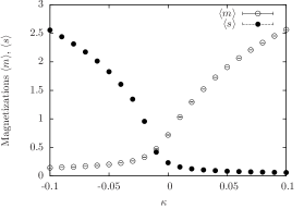 |
 |
 |
| (a) | (b) | (c) |
It is quite instructive to compare the effect caused by the aforementioned finite volume contributions to the obtained Monte-Carlo data. Meant as a quick and crude estimation the effective action , with given in Eq. (4.2.1), has therefore been evaluated at for the scalar field being restricted to the ansatz with defined in Eq. (4.7). Employing the results in Eq. (4.18) and Eq. (4.81) the expectation values and have then been estimated through the minima of the resulting expression for with respect to and . While this simple approach cannot correctly predict the phase transition of the model, it suffices to estimate the behaviour of and in the limit of large Yukawa coupling constants and large negative or positive values of the hopping parameter. This is demonstrated in Fig. 4.16, where the average magnetizations numerically obtained on the -lattice are presented again, this time, however, together with the aforementioned analytical estimate of the finite volume effects, depicted by the dashed lines. One then finds in Fig. 4.16 that the asymptotic behaviour of as well as the aforementioned asymmetry in and is well explainable already with this simple approach.
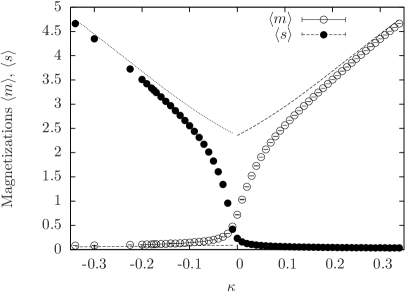 |
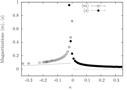 |
| (a) | (b) |
It is remarked that it is the term appearing in Eq. (4.81) that hinders from vanishing and induces the observed asymmetry. As already pointed out before this term as well as all other contributions arising from the -determinants in Eq. (4.2.1) are only finite volume contributions. As the volume increases the latter contributions loose their significance and the average magnetization becomes increasingly less influenced by the above logarithmic term, such that a symmetric phase can finally emerge. This is exactly what is observed in Fig. 4.15.
In Fig. 4.17 the susceptibilities corresponding to the magnetizations in Fig. 4.15 are presented. On the smallest lattice, i.e. the -lattice, one observes only one peak in the magnetic susceptibility, approximately centered at . From this result one might draw the conclusion that the phase transition point is located at , excluding a symmetric phase, since the staggered susceptibility reaches its maximum at the same value of . However, with increasing lattice sizes a second peak develops in the susceptibilities. This is very well observed in Fig. 4.16b corresponding to the larger -lattice. It is actually this second peak, approximately centered around in this case, that correctly describes the physical phase transition between the ferromagnetic and the symmetric phase, while the first one is only caused by the aforementioned finite volume effects. Its height is therefore expected to be constant in contrast to the physical peak, which grows with increasing lattice volume. On the largest presented lattice, the -lattice, the physical peak at completely dominates the scene and the former small volume peak at has disappeared, presumably hidden beneath the large error bars at .
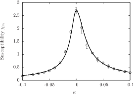 |
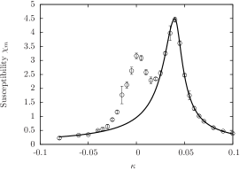 |
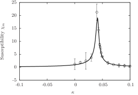 |
| (a) | (b) | (c) |
The SYM-FM phase transition points have then been determined by fitting the physical peaks in the magnetic susceptibility on the intermediate -lattice to the finite volume fit ansatz in Eq. (4.48) by taking only the points belonging to the physical peak into account as demonstrated in Fig. 4.17b. It is remarked that no results for the SYM-AFM phase transition are provided here, since this phase transition points have not been reliably detectable on the -lattice, due to the finite volume effects discussed above, and also not on the -lattice owing to a much larger numerical demand when performing the Monte-Carlo calculations in the anti-ferromagnetic phase with the naive implementation of the HMC-algorithm introduced in section 3.5.
In Fig. 4.18 the obtained phase transition points are presented together with the analytical infinite volume, large expectation of the phase structure at large values of the Yukawa coupling constant taken over from the preceding section. Qualitatively, the picture obtained from the numerical simulations is in full accordance with the results from the large approximation. There are second order phase transitions separating a ferromagnetic phase from a symmetric phase. In this symmetric phase strong finite size effects are encountered blocking its observation on too small lattice volumes. Here the order of the phase transition is identified to be of second order according to the continuous dependence of on the hopping parameter as demonstrated in Fig. 4.15. Again a more careful analysis is omitted here, since the considered phase transition is not in the main interest of the present study. Quantitatively, however, the numerical results deviate from the analytical expectation due to the finite settings and , but are still in relatively good agreement.
As a concluding remark one can summarize that a symmetric phase at large values of the Yukawa coupling constant does indeed exist although its existence is obscured on too small lattice volumes by strong finite size effects, and that its location within the phase diagram is in acceptable agreement with the analytical large predictions. The existence of a symmetric phase at strong Yukawa couplings has also been observed and discussed in LABEL:Giedt:2007qg. From these findings one can conclude that the phase structure of the considered Higgs-Yukawa model at large values of the Yukawa coupling constant is acceptably well described by the analytical large calculations presented in section 4.2.1.
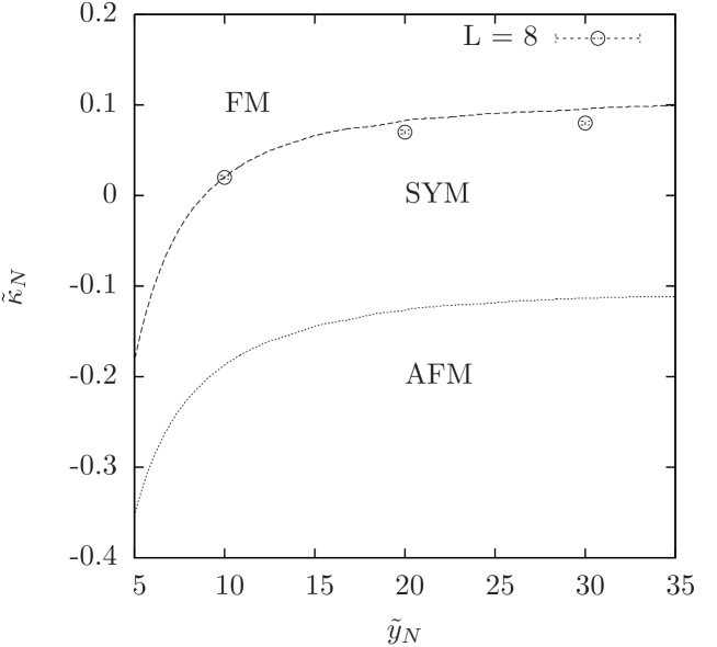
Chapter 5 The simulation algorithm
In the preceding chapter the HMC algorithm described in section 3.5, which is only applicable for even values of by construction, was used in order to check the validity of the analytical calculations performed in the large -limit. Since there is no need to consider odd values of to test the analytical large results, this easily implementable algorithm was fully sufficient for the given purpose. The numerical evaluation of the model in the physically relevant setup, however, requires a more advanced technique, for instance a PHMC [108, 151, 152] or a RHMC [153, 154] algorithm, which are both capable of dealing with odd values of . Here, a PHMC algorithm has therefore been implemented in addition to the previously employed HMC method. The basic concepts of this more advanced approach will shortly be summarized in section 5.1.
For the case of the considered Higgs-Yukawa model this standard algorithm could be enriched by a couple of technical enhancements. The most crucial improvements originate from the observation that the condition number of the fermion matrix can be reduced by about 1-2 orders of magnitude through the use of appropriate preconditioning techniques at least in the considered broken phase of the model, and that the auto-correlation times of the considered observables can be brought down from order to order by a technique known as Fourier acceleration [175, 176]. This will be discussed in sections 5.2 and 5.3, respectively. Furthermore, efficient techniques for an exact reweighting of the generated field configurations as well as the direct sampling of the pseudo fermion fields are presented in sections 5.4 and 5.5. The computational performance could additionally be improved by the use of a multiple time-scale integration scheme of the molecular dynamics underlying the PHMC algorithm, as demonstrated in section 5.6.
Moreover, a highly efficient implementation of a Fast Fourier Transformation (FFT) in four dimensions was implemented for the purpose of switching back and forth between the momentum and the position space representations of the pseudo fermion fields allowing then for a very efficient application of the Dirac operator as discussed in section 3.5. In the considered case of four dimensions and on sufficiently large lattice volumes this implementation is significantly more efficient on the employed hardware resources than the most widely spread standard implementation FFTW [155] as detailed in appendix B.
The aforementioned algorithmic improvements were crucial for the successful numerical evaluation of the model and shall therefore be presented in some detail here. In the following the applicability of these techniques will be discussed and tested in the framework of the physically relevant model parameter setups listed in Tab. 5.1, which cover the whole range of cutoff values that will be investigated in the later chapters dealing with the actual Higgs boson mass bound determination.
It is finally remarked, that some of the techniques discussed in the following, though only presented here for the case of the Higgs-Yukawa model, seem to be applicable to QCD as well.
5.1 The basic PHMC algorithm
The PHMC algorithm as well as its predecessor, the HMC algorithm, are both based on the fact, that the determinant of a hermitian and positive matrix can be written in terms of a Gaussian integral over some complex vector according to Eq. (3.85). As in the case of QCD the fermion matrix of the considered Higgs-Yukawa model, however, is not positive definite. The determinant of itself can therefore not be expressed in terms of such a Gaussian integration. The basic idea underlying both, the HMC as well as the PHMC algorithm, is to circumvent this problem by considering the positive and hermitian operator instead of . While this doubling of the fermion matrix is interpreted as a duplication of the number of fermions in the theory making this approach applicable in case of even numbers of degenerate fermions as discussed in section 3.5, the PHMC aims at correcting for the double counting.
This can be achieved by taking the square root of which is well defined due to the positivity and hermiticity of . One then arrives at the expression
| (5.1) |
for the partition function of the considered Higgs-Yukawa model which is fully equivalent to the definition in Eq. (3.42). The general idea of a PHMC (Polynomial Hybrid Monte-Carlo) algorithm is to make the square root of the operator numerically accessible by using polynomial approximations. More precisely, for a given polynomial of degree approximating the function , with maximal relative deviation
| (5.2) |
in the interval , the determinant can be transformed into a Gaussian integration times a real weight factor according to
| (5.3) | |||||
| (5.4) |
with the definition of the functional integral being111As usual constant factors have been neglected.
| (5.5) | |||||
| (5.6) |
which is suitable for numerical calculations as will be seen in the following. Here denotes a set of complex vectors referred to as pseudo fermion fields in the following, and the calculation of the complex phase has already been discussed in section 3.6. The expectation value of an observable is then given as
| (5.7) |
where the expectation value with respect to the modified dynamics arising from the polynomial alone, i.e. neglecting the weight factors, is given as
| (5.8) |
It is actually this latter functional integral that is computed in a PHMC algorithm. The multiplication of the considered observable with the weight factors according to Eq. (5.7), which is known as reweighting in the literature, then guarantees the PHMC algorithm to yield the correct result with respect to the full dynamics.
It is remarked at this point that the polynomial with the aforementioned properties can be constructed in numerous ways. In this implementation a least-square minimization procedure with respect to the residual with has been used, based on the software code published in LABEL:Gebert:2003pk. This method defines the scalar product of two given square-integrable, real functions , as
| (5.9) |
leading then to the corresponding norm . The squared norm of the residual
| (5.10) |
can then be minimized in the space of all polynomials with maximal degree by using the availability of a scalar product to project the function to a chosen basis of that space. Here, the inclusion of the factor in Eq. (5.9) and thus in the norm of the residual implicates an optimization with respect to the relative deviation, which is desirable for our purpose. The only difficulty is that this computation has to be performed with very high numerical precision to get stable results also in case of high polynomial degrees. For that purpose the code in LABEL:Gebert:2003pk employs some standard high precision numeric software library [178]. Furthermore, it is remarked that this approach relies on the fact that the scalar product of the considered function and any given polynomial as defined in Eq. (5.9) can be calculated analytically, since computing the respective integral numerically with the required accuracy is not very practicable.
For the numerical evaluation of the functional integral in Eq. (5.7) to yield stable results the weight factor should in general, apart from the exceptions in the next paragraph, fluctuate as little as possible. In the limit the weight converges to one and the fluctuations vanish provided that a sufficiently large approximation interval has been chosen such that all eigenvalues of the operator encountered in the Markov process are covered. Since decreasing or enlarging the approximation interval requires a higher degree of the underlying approximation polynomial there is always a trade-off between the fluctuation of and the computational resources needed to calculate .
While it is absolutely mandatory for the numerical stability of the algorithm that is a true upper bound for all eigenvalues of encountered in the Monte-Carlo process, the lower interval bound is allowed to be chosen larger than the smallest attainable eigenvalue, which would be corrected for by the reweighting factor . This freedom is often used to explicitly select a lower bound that is clearly larger than the lowest observed eigenvalue of . Though the resulting reduction of the required polynomial degree is accompanied with a higher fluctuation of this technique can reduce the overall numerical cost of the whole computation in the sense of achieved accuracy per numerical cost, in particular if there are only a few extremely small eigenvalues well separated from the rest of the eigenvalue spectrum [108]. It can also be advantageous when the considered observable itself fluctuates strongly, ideally anti-proportional to the smallest eigenvalue of like, for instance, the fermion propagator [108]. In the latter case choosing a larger does not only reduce the necessary polynomial degree but it also stabilizes the numerical calculation by compensating the fluctuation of such an observable with that of . In this work, however, a different reweighting approach is implemented. The details of this new reweighting technique will be given in section 5.4.
Concerning the practical evaluation of the matrix-valued polynomial a suitable representation for has to be chosen. A representation in terms of a Chebyshev basis is numerically very stable, but it does not directly allow for the calculation of the forces needed for the integration of the molecular dynamics equations of motion as discussed in section 3.5. A decomposition in terms of monomials given as
| (5.11) |
where the complex numbers denote the roots of the polynomial , provides a direct approach for calculating the aforementioned molecular forces according to
| (5.12) |
with
| (5.13) |
The evaluation of this latter expression requires no more than applications of the operator for each pseudo fermion field , provided that enough computer memory is available to store a number of auxiliary vectors.
The problem with this naive representation of in terms of monomials is its high numerical instability. This disadvantage can be cured by selecting an appropriate order of the roots and thus of the corresponding monomials. Different ordering schemes have been examined in the literature and the so-called bit-reversed ordering was found to yield very stable results [179]. This is the approach that will also be used in this implementation of the PHMC algorithm.
The Markov step for the field is then constructed in the same way as for the HMC algorithm by introducing the momenta conjugate to , integrating the equations of motions in terms of and with denoting the Monte-Carlo time, and accepting or rejecting the proposed configuration according to a final Metropolis step as described in section 3.5. The technique for the direct sampling of the pseudo fermion fields also differs from the one used in the HMC algorithm and will be discussed in section 5.5.
Finally, it shall be remarked that instead of the introduction of pseudo fermion fields in Eq. (5.1) one could also have used only one pseudo fermion field together with a polynomial approximating the function . It has, however, been discussed in the literature [180], at least for the case of the RHMC algorithm, that this approach should be less efficient than the chosen method due to larger force strengths encountered in the integration of the molecular dynamics and – translated into the framework of the PHMC algorithm – the requirement for a higher degree of the approximation polynomial for fixed relative accuracy .
5.2 Reducing the fermion matrix condition number through preconditioning
The condition number of the fermion matrix has a tremendous impact on the overall numerical cost of the lattice calculations performed in this study. For a general, diagonalizable matrix it is given as the norm of the ratio of the eigenvalue with largest norm divided by the eigenvalue with smallest norm according to
| (5.14) |
This quantity strongly influences the asymptotic convergence speed of many numerical algorithms. For the conjugate gradient (CG) algorithm, used in the HMC approach to apply the inverse of on a given vector, the norm of the residual goes to zero proportional to for sufficiently large iteration numbers . In case of the polynomial approximation used in the PHMC algorithm the condition number specifies the size of the approximation interval , more precisely the ratio , needed to cover the whole eigenvalue spectrum of . Thus, it is directly related to the numerical cost for the evaluation of the polynomial . The condition number also influences the convergence speed of the Arnoldi algorithm used to determine the sign of the fermion determinant as described in section 3.6.
The main idea of this section is to reduce the numerical cost of the intended lattice calculations by reducing the condition number of the fermion matrix. To be more precise, the fermion matrix will be replaced by some other matrix, which generates exactly the same physical results but possesses a lower condition number. This is possible, at least in the broken phase of the model, which is the scenario that underlies all considerations in the following. In section 5.2.1 this approach will be discussed for and applied to the fermion matrix itself in the context of reducing the computational costs for the determination of the sign of the fermion determinant . Since the identical approach will not work for the squared operator , a somewhat different ansatz will be presented in section 5.2.2 capable of cutting down the condition number of by orders of magnitude, thus leading to an outstanding performance gain in the later lattice calculations.
5.2.1 Preconditioning of
Based on the observation in section 3.6.1 that the general structure of the eigenvalue spectrum of is very much determined by the eigenvalue spectrum of the free Dirac operator as well as the magnetization of the underlying field configuration the basic idea here is to use the analytically invertible operator to precondition the general fermion matrix , where the field has been given in Eq. (4.7) and consists solely of a constant and a staggered mode as specified by the amplitudes222The notation in this chapter differs from that in chapter 4. The hat symbols of , underlying the definition of in Eq. (4.7) are omitted and the factor in the definition of will always be divided out, such that the observables , evaluated on equal , . , and the orientations , . For that purpose the preconditioning operator is defined as
| (5.15) |
The obvious expectation is that the product should be close to the identity provided that the parameters , of the matrix match the magnetizations333Here and in the following it is always assumed that at least one of the two magnetizations , is non-zero. , of the field configuration underlying the operator and that the orientations , point into the directions and , respectively. Consequently, the condition number is supposed to be close to one, at least in the broken phases. For simplicity, however, a restricted ansatz is employed in the following given as
| (5.16) |
which turns out to be still sufficiently good for the considered purpose here.
This approach seems promising for the determination of the sign of the fermion determinant . The reason is that the numerical cost for the computation of the eigenvalues of should be reduced due to its condition number being smaller than . At the same time the phase, and thus the sign, of the determinant is unaltered by the multiplication with the operator , i.e.
| (5.17) |
according to
| (5.18) |
The latter result is easily obtained by employing the exactly known eigenvalue spectrum of for some non-zero value . For the sake of completeness it is remarked that in the case of exactly zero magnetization, i.e. , the latter quantity can not be employed to precondition the fermion matrix due to . However, the set is a set of zero measure and will moreover practically not occur when investigating the broken phase as intended. Furthermore, it is straightforward to test for this condition in the program code to avoid the application of the preconditioning technique in that scenario.
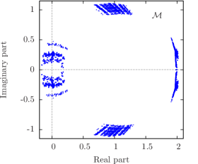 |
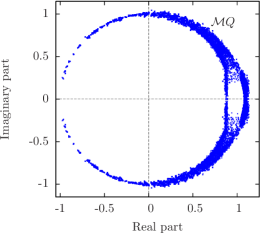 |
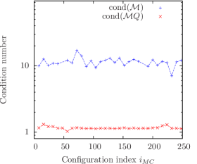 |
| (a) | (b) | (c) |
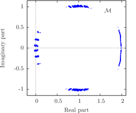 |
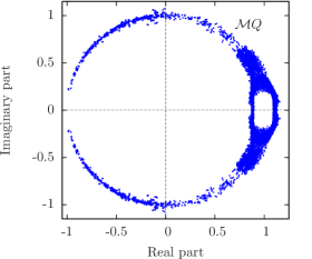 |
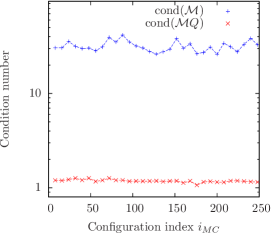 |
| (d) | (e) | (f) |
The applicability of this approach is demonstrated in Fig. 5.1. The results presented there have been obtained in Monte-Carlo runs performed on -lattices in the broken phase, selected to give a typical example of the improvement that has been achieved. The plots in panels (a,b,d,e) each show a superposition of eigenvalues determined on several field configurations. Since the full spectrum cannot be computed for practical reasons, only 120 eigenvalues have been computed on each field configuration, equally composed out of those eigenvalues with smallest norm, largest norm, smallest and largest real part, as well as smallest and largest imaginary part, which could be achieved with the help of an implementation [164] of the Arnoldi algorithm. The intention of this presentation is to provide an illustration of the eigenvalue spectrum of the respectively considered operators.
In panels (a,d) this has been done for the fermion operator itself and one clearly observes the circular base structure inherited from the free Neuberger operator . In contrast, the eigenvalue structure of the matrix presented in panels (b,e) looks very much distinct. The eigenvalues no longer lie on the Neuberger circle passing through the origin, but rather on the unit circle. The results for the corresponding condition numbers are presented in Fig. 5.1c,f. The condition number is distinctly smaller than that of the original fermion matrix and fluctuates very close to one as intended.
However, the convergence speed of the Arnoldi algorithm is not solely determined by the condition number but also by the eigenvalue density and other factors. Besides that the approach to determine the sign of the fermion determinant described in section 3.6.1 depends very much on the average number of eigenvalues situated in the complex half-plane with negative real part. The actual reduction of the numerical cost of the procedure to compute the sign of the fermion determinant should therefore be tested explicitly. In Tab. 5.2 the resulting average computation times for determining with and without the usage of the preconditioning matrix are compared to each other. One sees that speed-up factors around 1-2 orders of magnitude can be achieved by this approach in practice.
| Monte-Carlo run | Avg. time for | Avg. time for |
|---|---|---|
| minutes | minutes | |
| minutes | minutes |
5.2.2 Preconditioning of
With the results of the previous section in mind it would be extremely desirable to exploit the benefits of the low condition number of also in the actual PHMC algorithm itself where the condition number of the squared operator determines the computational cost. Indeed, a partition function being equivalent to Eq. (5.1) can be constructed based on the assumedly improved operator according to
| (5.19) |
where the preconditioning parameter is held constant during the whole Monte-Carlo calculation. It should be noted here, that there is no correction factor needed for the inclusion of the operator . This is because the parameter is fixed, such that the determinant only gives a constant factor independent of the actual field configuration . The idea here is to fix the parameter at the start of the Monte-Carlo computation, such that it matches the average magnetization, i.e. . This, of course, involves some small amount of tuning.
From the experience of the previous section one might then expect the condition number to be of the order of the square of , i.e. of order according to the examples presented in Fig. 5.1c,f.
This, however, is not the case. In fact, the condition number can even be much larger than the one of the unpreconditioned operator , as demonstrated in Fig. 5.2a and Fig. 5.2b for identically the same Monte-Carlo runs that served as the example setup in the preceding section. This is not a result of fixing the preconditioning parameter to . To clarify this the condition numbers of the preconditioned operator have been determined here by setting the parameter individually to the respective magnetization for each evaluated configuration, i.e. is presented in Fig. 5.2.
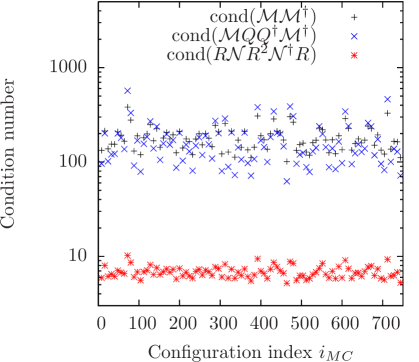 |
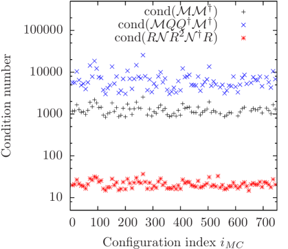 |
| (a) | (b) |
The reason for this outcome originates from the fact that the fermion matrix is not hermitian. In fact, the operators and do not even share a common eigenvector basis. This statement is also inherited to the matrices and . In this general setup the condition number of a product of matrices is not the product of their condition numbers, i.e.
| (5.20) |
which explains the observation in Fig. 5.2. The naive approach given in Eq. (5.19) must therefore be considered to have failed.
To elaborate on a potential cure to this unsatisfactory finding, we consider the following Gedanken experiment. We now assume to have a -independent, non-singular, hermitian matrix with at hand, such that is hermitian. In case of QCD such an operator is given by due to the -hermiticity of the QCD fermion matrix. Moreover, we assume that the condition number is small, which is plausible due to the definition of the latter hermitian operator given here as
| (5.21) |
Postulating that is non-singular, which is indeed the case according to the above definition, provided that as already discussed in the preceding section, one directly finds
| (5.22) |
and thus
| (5.23) |
due to the hermiticity of . Exploiting the fact that commutes444One directly finds when exploiting , which holds for the space-time independent field underlying the definition of in Eq. (5.21). with according to the specific definition of in Eq. (5.21) one can further simplify the above expression to
| (5.24) |
where the hermitian, positive matrix is defined as
| (5.25) | |||||
| (5.26) |
Moreover, one has
| (5.27) |
up to a -independent factor, provided that the constant parameter is non-zero. Following the same arguments given at the beginning of this section the Monte-Carlo calculation could thus be based on the latter well conditioned operator having a condition number of only in the here considered hypothetical scenario.
However, when actually trying to apply this strategy to the considered Higgs-Yukawa model, one faces the problem of finding an operator with the aforementioned properties. Since is not -hermitian, as discussed in section 3.6, the setting is not an eligible choice here. In fact, the fermion matrix would not even be -hermitian, when the three components , , and of a given field configuration would be identical to zero and only would be non-constant over space-time. The origin of these bad hermiticity properties lies in the pronounced asymmetry of the fermion matrix
| (5.28) |
A potential cure to this problem would be the construction of a new fermion matrix having better symmetry properties, with respect to a -hermiticity for instance, while still producing the same physics. The idea would then be to precondition the modified operator following the above strategy.
The latter requirement of producing the same physics is exactly fulfilled, if the determinant of equals that of the new operator for all field configurations up to a constant factor independent of . An example of such an operator is
| (5.29) |
where the matrix has been defined in Eq. (4.55) and the projector was given in Eq. (4.52). As desired the operator then fulfills
| (5.30) |
up to a constant factor, as can be seen by employing the relation in Eq. (4.2.1). In contrast to this new operator is -hermitian provided that the three components , , and of a given field configuration would be identical to zero and only would be non-trivial. Moreover, in the degenerate case with equal Yukawa coupling constants, i.e. , the matrix is -hermitian provided that only the component of the underlying field configuration is identical to zero. From these observations one may conjecture that the operator is a more promising candidate for reducing the computational cost according to the strategy described above.
Though the newly introduced operator does also not – at least not obviously – obey an exact -hermiticity relation in the general situation, we nevertheless apply the above preconditioning strategy. The next step is thus the definition of the preconditioning matrix for the new operator according to Eq. (5.26) yielding the definition
| (5.31) |
The expectation is now that the composed operator possesses a distinctly smaller condition number as compared to .
That this is indeed the case can be observed in Fig. 5.2 where the condition number is presented for exactly the same configurations underlying also the aforementioned results for and . In comparison with the operator the condition number of the improved operator has been reduced by a factor of around 1-2 orders of magnitude.
However, one may ask whether this technique is restricted to the case of degenerate Yukawa coupling parameters, which have been assumed so far. Furthermore one may ask whether the success of this approach is related to the already relatively small condition numbers of the initial operator presented in Fig. 5.2. To answer these questions an additional example is given in Fig. 5.3. The configurations underlying this demonstration have been obtained in a Monte-Carlo run with corresponding to the physical ratio of the bottom and top quark mass. Moreover, the condition numbers of the initial operator are significantly larger now than in the previously presented examples. Still the condition numbers of the operator are improved by 1-2 orders of magnitude as compared to the case of the original operator .
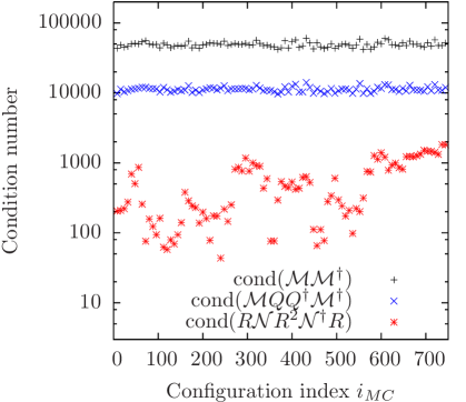
For the purpose of clarification let us shortly summarize the partition function we found to be most suitable for the the numerical calculations so far. Up to some constant factor the partition function in Eq. (5.3) is equivalent to
| (5.32) | |||||
| (5.33) |
with the definition of the functional integral being
| (5.34) |
where the preconditioning matrix is held constant over the whole Monte-Carlo run and is intended to be fixed to . This approach produces exactly the same dynamics as Eq. (5.3) does, but is more favorable from a numerical point of view due to the much smaller condition number of the operator as compared to .
For completeness it is remarked that the actually relevant quantity determining the necessary size of the underlying approximation interval in a PHMC algorithm is not the observed maximal value of the condition number itself, but rather the ratio of the largest and smallest eigenvalues observed in the whole Markov process given as
| (5.35) |
where the respective maximizations and minimizations are performed over all generated field configurations and over all eigenvalues of the underlying fermion operator. This measure generally differs from the observed maximal value of the condition number, since the largest eigenvalue associated to a given field configuration and a given fermion operator fluctuates during the Monte-Carlo process. The results on for the original and the preconditioned fermion operators as obtained in the same example Monte-Carlo runs already considered before are listed in Tab. 5.3. From this presentation one can also learn that some fraction of the gained improvement of the condition number as compared to is lost by the requirement that the preconditioning parameter must be fixed.
However, the relevant quantity of the operator is still reduced by a typically factor of around in comparison to the corresponding finding of the original matrix as can be seen in Tab. 5.3.
| Example setup | |||||
|---|---|---|---|---|---|
| Operator | |||||
| 618.1 | 152 | ||||
| 13.9 | – | – | – | ||
| 25.1 | 30 | ||||
| 2561.8 | 310 | ||||
| 67.0 | – | – | – | ||
| 121.4 | 66 | ||||
| 619994.6 | 1520 | ||||
| 1992.8 | – | – | – | ||
| 2268.4 | 292 | ||||
To illustrate the actual impact of the achieved reduction of the fermion matrix condition numbers on the computational cost for the evaluation of the polynomial , or rather in the improved case, a couple of example setups for the approximation polynomial typically chosen for the observed value of are presented in Tab. 5.3. In these example setups the ratio of the approximation interval boundaries was chosen such that the whole observed eigenvalue spectrum is covered. The presented value of the polynomial degree is given here as the minimal even degree fulfilling the criterion of the associated maximal relative deviation , which will turn out to be a reasonable choice in section 5.4 still leading to an exact algorithm.
One can observe in the presented listing that the polynomial degree , specified in the above manner, decreases quickly when the approximation interval is reduced while the requested maximal relative deviation is held constant. From the presented numbers one finds that the achieved reduction of the quantity typically translates into a decrease of the required polynomial degree by a factor of around . Since the computation of the matrix-valued polynomial consumes the major portion of the numerical resources, this achieved reduction of the polynomial degree turns, for the most part, into an overall improvement factor of the whole Monte-Carlo calculation.
Concerning the applicability of the here considered preconditioning technique also in the case of QCD one faces the problem that a pendant of the here exploited correlation between the eigenvectors of the general fermion matrix and those of does apparently not exist in the case of QCD due to its local gauge invariance. The presented approach can therefore not directly be applied to the case of QCD, unless one succeeds to establish the aforementioned correlation, for instance, by means of gauge fixing procedures. While such an approach does not seem to be practical for the Markov process of generating the gauge field configurations itself, it might be interesting for the analysis of the latter field configurations with respect to the calculation of the fermion propagators, which requires a large number of fermion matrix inversions for each single gauge field configuration but only one gauge fixing procedure.
5.3 Reducing auto-correlation times through Fourier acceleration
The auto-correlation time is a measure for the statistical correlation of the configurations generated in a Monte-Carlo process. It can roughly be interpreted as the number of subsequent configurations, which have to be considered as statistically dependent. More precisely, the auto-correlation time as defined in the following is not a direct property of the field configurations alone but depends also on the choice of the considered observable . The true performance of a simulation algorithm in the sense of achieved accuracy of the numerical result on per computation time is thus not only determined by the run-time speed itself, i.e. by the number of configurations generated in a given computation time, but also by the auto-correlation time of the considered observable.
This section intends to demonstrate how the method of Fourier acceleration555Special thanks go to Prof. Julius Kuti and to Chris Schroeder for pointing out the Fourier acceleration technique to me. Its applicability to a similar Higgs-Yukawa model has moreover been demonstrated in LABEL:Schroeder:2007zu. [175, 176] can be adopted to the considered Higgs-Yukawa model in order to reduce the encountered auto-correlation times of the considered observables, thus increasing the overall performance of the implemented simulation algorithm. For that purpose we start here with a more precise definition of the auto-correlation time .
As discussed in section 3.5 the general strategy for calculating the expectation value of an observable in the Monte-Carlo approach is to estimate that quantity by the ensemble average obtained from a given finite set of field configurations according to Eq. (3.90-3.92). In the case of statistically independent samples the variance of would be given by , where denotes the standard deviation of the single measurements , . In practice, however, the field configurations generated in the Monte-Carlo process, and thus the corresponding measurements , are highly correlated, unless some method of direct sampling was used. For the error analysis it is therefore of great importance to consider the correlation among the obtained measurements to obtain a reliable error estimate for the ensemble average , and thus for the estimate of .
Starting from the definition of the variance of the ensemble average being
| (5.36) |
where the assumed unbiasedness of the estimate of through has already been used, one directly arrives at the result that the variance still scales proportional to but with a proportionality constant instead of according to
| (5.37) | |||||
| (5.38) |
where terms of the order have been neglected and the actually finite summation in Eq. (5.37) has been extended to an infinite sum, which is well justified, since one usually has . Moreover, the definition in Eq. (5.38) only makes sense for which, however, is an irrelevant restriction in practice for the same reason. It is further remarked that one finds in the case of complete statistical independence and thus recovering the prior result.
In a practical determination of , however, all expectation values in Eq. (5.38) have to be replaced by corresponding ensemble averages. Moreover, the window size , in which the function is to be summed up, typically has to be set to a finite value , since the determination of the correlation function becomes statistically unstable at large separations . Choosing an appropriate value for is thus a trade-off between the latter statistical uncertainty on the one hand and the systematic neglection of long-ranged correlations on the other hand. For a reliable determination of one usually requests the observation of a plateau in the function and takes its plateau value as an approximation for . This whole procedure is well known as the -strategy [182] in the literature.
The auto-correlation time is then defined through the decay rate of the expected exponential behaviour of the correlation function according to
| (5.39) |
It is thus directly connected to via
| (5.40) |
which simplifies in the case of to
| (5.41) |
A typical example for an observable with very large auto-correlation time is presented in Fig. 5.4a. Here, the magnetization has been selected as the considered observable. The corresponding auto-correlation time, expressed in terms of the function , is depicted in Fig. 5.4b. The presented data have been obtained in a PHMC calculation without applying any of the enhancement procedures which will be discussed in this section. For the given example one finds the auto-correlation time of the underlying observable to be of order which is a typical value for the chosen observable and the selected lattice volume. Such a large auto-correlation time obviously poses a severe difficulty for the reliable calculation of the expectation value of this observable.
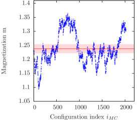 |
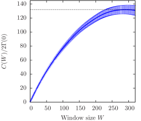 |
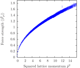 |
| (a) | (b) | (c) |
It is well known that observables dominated by low momentum modes generally suffer the most from large auto-correlation times, as can be formally shown at least for the free theory [183]. The auto-correlation time of the observable , which purely reflects the amplitudes of the zero-momentum modes of the scalar field , can therefore be considered as a good indicator for the worst observable auto-correlation time in a given Monte-Carlo run. This is why we will mainly consider the magnetization as the underlying observable for the analysis of the auto-correlation time in the following.
The origin of these extremely bad auto-correlation properties can be observed in Fig. 5.4c. This plot shows the numerically calculated average molecular force in momentum space defined as
| (5.42) |
versus the squared lattice momentum of the respective mode it is acting on. Interestingly, a very pronounced relation between and the associated force is observed. The long auto-correlation times of the magnetization can directly be ascribed to the minimum of the measured average forces being located at . The much larger forces acting on the higher momentum modes, on the other hand, are the main sources for the discretization errors encountered in the numerical integration of the molecular dynamics equations of motion. The step size of the numerical integrator has thus to be adjusted to sufficiently small values to allow for a stable integration of these high-momentum modes, while the very same modes do not contribute to the considered observable at all. In fact, this is the general situation, which can, however, be more or less pronounced depending on the considered observable. The reasoning is that the low momentum modes determine the long-range physics, which we are mainly interested in when performing the later lattice calculations. These low momentum modes, however, evolve the slowest in the unimproved Monte-Carlo algorithm considered so far.
A well-known cure to the described problem is the Fourier-Acceleration technique [175, 176]. Its main idea is to assign different effective trajectory lengths to the momentum modes, such that the low momentum modes see an enlengthened effective trajectory length during the integration of the equations of motion. For that purpose a fictitious mass is introduced for each momentum mode, in such a way that those modes with smaller assigned masses move faster during the integration process. This can be achieved by replacing the standard setting for the function , which determines the sampling of the conjugate momenta according to Eq. (3.97), with some more appropriate choice incorporating the latter fictitious masses according to
| (5.43) |
where denotes the Fourier transform of the conjugate momenta given as
| (5.44) |
Obviously, the introduction of the aforementioned masses does not influence the physical results obtained with this new choice of the function as discussed in section 3.5. To understand the effect of these fictitious masses let us consider a solution of the Fourier-accelerated equations of motion associated to the function according to Eq. (3.106-3.108). This solution fulfills
| (5.45) | |||||
| (5.46) |
where the here omitted pseudo fermion fields are again assumed not to propagate during the integration step. We now define the rescaled momenta , such that is Gauss-distributed with standard deviation one as it is the case for the original momenta sampled according to the standard choice . The trajectory then solves the differential equations666For the sake of brevity the inner mappings and are implicit here.
| (5.47) | |||||
| (5.48) |
which coincide with the original equations of motion in the unimproved scenario given in Eq. (3.106-3.108) differing only through the replacement . Integrating Eq. (5.45-5.46) from to , which is actually done in the simulation algorithm, would thus formally correspond to an integration of the momentum modes in Eq. (5.47-5.48) from to , respectively, explaining the notion of the momentum dependent, effective trajectory length
| (5.49) |
The vital question is how these effective trajectory lengths and thus the fictitious masses should be chosen. Here, it is intended to determine such that the momenta , resulting from the Gaussian sampling according to the distribution in Eq. (5.43), are of the same scale as the corresponding forces , which would be a ’natural’ situation. We thus choose the fictitious masses as
| (5.50) |
where the specified factor is purely conventional, translating into an overall, momentum independent boost of the effective trajectory lengths only. In a practical lattice calculation the average forces can simply be measured in the early phase of the thermalization process of the Monte-Carlo run before the Fourier acceleration is finally switched777Switching the Fourier acceleration on and off simply refers to setting the momentum masses to the setting in Eq. (5.50) or to , recovering then the usual, unimproved equations of motion. on. For stability reasons one should, however, define a maximal effective trajectory length that will not be exceeded. For the most performed lattice calculations in this work the relative prolongation of the effective trajectory lengths with respect to the nominal value has been restricted to .
The effect of the presented Fourier acceleration technique shall now tested. For that purpose the Monte-Carlo run that produced the results presented in Fig. 5.4 was repeated with the same parameter settings, but activated Fourier acceleration technique, i.e. with the choice of the function according to Eq. (5.43) and employing the corresponding equations of motion listed in Eq. (5.45-5.46). The obtained results for the measured magnetizations are presented in Fig. 5.5a while panel (b) shows the associated auto-correlation time of that observable in terms of the function resulting from this improved approach. The underlying choice of the momentum dependent, effective trajectory lengths in relation to the nominal value is shown in Fig. 5.5c. One finds from these results that the benefit of the Fourier acceleration technique is excellent for the given example. The auto-correlation time could be reduced by a factor of the order , which is a typical finding for the given lattice volume in the considered regime of small Yukawa and quartic coupling constants.
It is remarked at this point that the Fourier acceleration technique is also applicable in the case of an infinite quartic self-coupling constant. In this scenario the field variables are each constraint to a sphere. Again, effective trajectory lengths can be assigned to the different momentum modes by the introduction of fictitious masses according to Eq. (5.43) with the only difference that in this case the conjugate momenta possess only three components , . A possible choice for the equations of motions leaving the action invariant is then given by
| (5.51) | |||||
| (5.52) |
where the same notation as in section 3.5 has been used. Again the movement in the would-be component is implicitly projected out in Eq. (5.52) and the given differential equation in Eq. (5.51) can be solved exactly for constant leading then to the finite step size result
| (5.53) |
which is applied in the actual numerical implementation to fulfill the constraint on the field exactly. The construction of a suitable numerical integration scheme is then fully analogue to that presented in section 3.5.
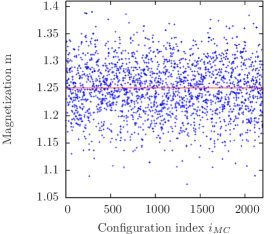 |
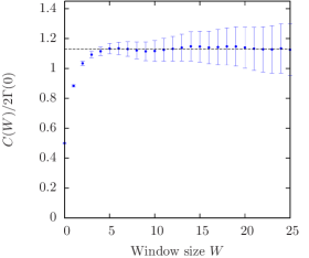 |
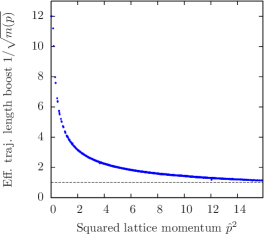 |
| (a) | (b) | (c) |
An example for the benefit of the Fourier acceleration technique at infinite quartic self-coupling constant is given in Fig. 5.6a, where the auto-correlation times of the magnetization obtained in two Monte-Carlo runs with the same parameter settings differing only through the usage or non-usage, respectively, of the presented improvement technique are compared to each other. The auto-correlation time obtained for deactivated Fourier acceleration technique is much larger than that measured in the case of activated Fourier acceleration. The attainable improvement factor, being approximately in this example, is typically found to be smaller than in the prior case of small coupling constants. However, the achieved improvement is still crucial for the successful evaluation of the considered model in the regime of strong quartic coupling constants.
To provide an even clearer picture of what has been achieved the auto-correlation times of the Higgs propagator, i.e. of the observable , are shown in Fig. 5.6b and Fig. 5.6c versus the squared lattice momentum . These results are taken from the same Fourier-accelerated Monte-Carlo runs that have already served as examples before. One observes that the presented auto-correlation times are more or less independent of the momentum . Moreover, one sees that almost all auto-correlation times fluctuate around a value of in the given examples. Only the low momentum modes exhibit a somewhat larger value of , which is a remnant of the original situation where the zero momentum mode is clearly the slowest mode of all.
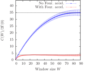 |
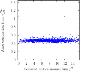 |
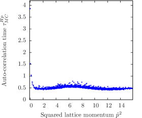 |
| (a) | (b) | (c) |
For completeness it shall be remarked here that the case of finite but arbitrarily large quartic coupling constant can also be treated very efficiently. In this scenario the field variables are not exactly constraint to a sphere. The application of the equations of motion in Eq. (5.51-5.52) would thus not lead to an ergodic algorithm, while the application of Eq. (5.45-5.46), on the other hand, would result in extremely small required step sizes of the numerical integrator due to the almost-constraint induced by . A possible solution to this problem would be to split up the dynamics of the field into a tangential and a radial movement and to assign different fictitious masses to either of them. Here, however, an even simpler approach is implemented. For that purpose the conjugate momenta are extended to a seven-component field and the Fourier accelerated version of the function is given as
| (5.54) |
Corresponding equations of motion can then easily be derived. The differential equations given as
| (5.55) | |||||
| (5.56) | |||||
| (5.57) |
hold the total action constant and are thus chosen in this approach. Here, the would-be -movement in Eq. (5.57) is again implicitly projected out and the quantities , are defined as
| (5.58) | |||||
| (5.59) |
The momentum dependent fictitious masses can then be determined such that the tangential movement of the field variables is boosted to a desired speed, while the momenta generate the missing radial movement, which can be adjusted to be arbitrarily slow via the masses . In the implemented approach, the tangential masses are chosen according to Eq. (5.50) and the fictitious masses are set to , where is a positive real number that determines the ratio of the effective trajectory lengths of the respective unconstrained movement and the tangential movement.
The resulting algorithm is then ergodic, yields low auto-correlation times, and the numerical cost of the integration scheme does not diverge as the finite quartic coupling constant is sent to infinity, provided that the fictitious masses are properly adapted in that limit. It is this method that will later be used to evaluate the model at large quartic coupling constants, for instance at , which would be rather problematic with the original approach.
As a technical remark it is added that one should project out the radial components of the force with respect to the radial direction given by at each space-time point , when determining the fictitious masses according to Eq. (5.50). Otherwise these masses would be influenced by force components that actually do not act on the conjugate momenta . With the same rationale this remark also applies to the previously discussed scenario of an infinite quartic self-coupling constant.
The alert reader might now wonder whether the reversibility of the integration scheme might be disturbed due to positive Lyapunov exponents of the integrator [184, 185, 186] and the enlengthened trajectory lengths. The effective trajectory lengths of the modes are, however, increased according to the force strength acting on that respective mode, i.e. the most boosted trajectory lengths are assigned to the originally slowest modes. Furthermore, the reversibility of the integration scheme was monitored during the simulation runs but no worrisome changes of the reversibility properties have been observed. This monitoring was done by periodically performing test integrations during the simulation where an integration was followed by an integration with reversed momenta. This allows to interpret the difference between the final field configuration obtained after the two numerical integration processes and the original field configuration as a measure for the reversibility of the applied integration scheme. The exact definition of this reversibility measure is given as
| (5.60) |
Typical examples of the latter quantity are given in Fig. 5.7 as obtained in the same Monte-Carlo runs that have already been considered before. This measure was evaluated for both, the Fourier accelerated as well as in the unimproved Monte-Carlo runs. From the presented findings one can conclude that the negative effect of the Fourier acceleration technique on the reversibility properties of the underlying numerical integrator, though clearly detectable by means of the considered quantity, is still in an acceptable range from a practical point of view.
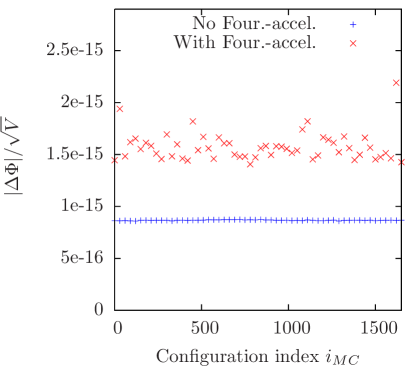 |
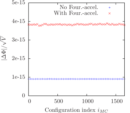 |
| (a) | (b) |
Furthermore, one may ask whether the achieved improvement in the auto-correlation time might be eaten up by a reduced acceptance rate in the Metropolis accept/reject step caused by the enlengthened effective trajectory lengths . Indeed, the acceptance rate is affected and a smaller step size is required in the integration scheme to compensate for that. The benefit of the reduced auto-correlation, however, clearly overweighs this drawback as demonstrated in Tab. 5.4, showing the measure for the numerical costs of the numerical integration as observed in a series of Monte-Carlo runs performed with and without the use of Fourier acceleration. The aforementioned measure is defined here as
| (5.61) |
where denotes the number of force evaluations required for the integration of one trajectory and the average acceptance rate was tuned to be the smallest adjustable value above by varying the number of integration steps for a given trajectory length .
In fact, one learns from the listing in Tab. 5.4 that the increase of the global trajectory length is generally advantageous, also independently of the framework of Fourier acceleration, provided that the reversibility of the integrator is not lost, which has also been observed in the case of QCD [187]. This can be understood, at least for the here considered Higgs-Yukawa model, by considering the (P)HMC-update of the field as a random walk in the high-dimensional configuration space. In this scenario the field configuration would have propagated the distance in configuration space after update steps with denoting the average size of a single update step, i.e. the update generated by a single integration of the equations of motion from to . If one interprets the auto-correlation time as the number of update steps necessary to propagate from one field configuration to the next statistically independent configuration, where statistical independence shall here be understood as a sufficiently large distance between the latter configurations in configuration space, then one would expect the auto-correlation time to scale proportional to and thus
| (5.62) |
The necessary decrease of the integrator step size accompanying an enlengthening of the trajectory length, however, scales only with where is the order of the selected integration scheme, i.e. for the leap-frog scheme. The pure cost of the integration scheme, neglecting the varying auto-correlation time, thus scales proportional to , leading to the scaling behaviour for the total numerical cost measure including the effect on the auto-correlation time. This explains why it is expected to be advantageous to increase the global trajectory length under the aforementioned conditions, assuming that .
Examples for the actually observed scaling behaviour of the auto-correlation time and the numerical cost measure with respect to the global trajectory length are presented in Tab. 5.4. One finds that the auto-correlation time approximately scales in agreement with the estimate in Eq. (5.62) for the unimproved Monte-Carlo runs. The numerical cost measures given in this listing also behave roughly as expected.
In fact, the presented Fourier acceleration technique is based on these observations. In contrast to a naive increase of the global trajectory length , however, the Fourier acceleration technique influences the effective trajectory lengths individually, in dependence on the original speed of the respective modes, minimizing thus the associated negative effects on the numerical costs and the numerical stability. The Fourier acceleration technique is thus superior to the naive increase of the global trajectory length as can be seen in Tab. 5.4. It is therefore the method of choice in the final implementation of the PHMC algorithm.
| FACC | ||||||
|---|---|---|---|---|---|---|
| No | 1.0 | 20120 | ||||
| No | 2.0 | 2020 | ||||
| No | 4.0 | 2120 | ||||
| Yes | 2.0 | 21780 | ||||
| No | 0.5 | 2020 | ||||
| No | 1.0 | 2580 | ||||
| No | 2.0 | 2100 | ||||
| Yes | 1.0 | 22360 |
Concerning the applicability of the Fourier acceleration technique also in the case of QCD one faces the problem that the exploited correlation between the force strength and the momentum modes does apparently not exit in the case of QCD due to its local gauge invariance. The here presented technique can therefore not directly be applied to QCD.
5.4 Krylov-space based exact reweighting
As already pointed out in section 5.1 the PHMC algorithm requires the consideration of a weight factor for each generated field configuration to guarantee its correctness. This is due to the finite degree, and thus finite accuracy of the chosen approximation polynomial888For simplicity will be used here and in the following as a placeholder standing for itself or its preconditioned version introduced in section 5.2.2 which is actually used in the implementation of the PHMC algorithm. . A second source for the necessity of reweighting the generated configurations is the finite extent of the approximation interval , unless it is guaranteed by some specific boundary that the eigenvalue spectrum of is constrained to the chosen interval. The reason is that there is no boundary at all for the deviation between the polynomial and the approximated function outside the specified approximation interval.
The definition of this weight factor has already been given in Eq. (5.4). In the literature one finds basically two different standard approaches to evaluate this reweighting factor, both of which can be performed separately from the actual generation of the field configurations in the Monte-Carlo process. The first is based on rewriting the determinant in Eq. (5.4) in terms of a Gaussian integration over some complex vector according to
| (5.63) | |||||
| (5.64) | |||||
| (5.65) |
where constant factors have been neglected, the usual setting has been assumed, and the functional integral is defined as
| (5.66) |
The weight factor can then be computed by means of a Monte-Carlo integration through randomly sampling a number of evaluation points where the integrand is to be evaluated. More precisely, the integral representation of the determinant in Eq. (5.63) has been split up here into a Gaussian factor , according to which the evaluation points, i.e. the complex vectors , are sampled, and the corresponding remaining factor , that has to be evaluated for the selected sampling points. In the given decomposition the numerical estimate of is then given as the resulting ensemble average. This approach is very well applicable in practice, since the expression is close to one by construction.
The second method is based on an exact computation of all eigenvalues , of with . The idea here is to use an approximation polynomial with sufficiently high degree such that the approximation can be considered to be exact within the interval . This is a reasonable assumption, if the maximal relative deviation is sufficiently small, ideally of the order of the machine precision. In this scenario the weight factor is given as
| (5.67) |
Both presented approaches have their specific advantages and disadvantages. The first ansatz has the very useful benefit that it allows to perform the actual Monte-Carlo calculation with a rather low degree of the approximation polynomial, speeding up the actual generation of the field configurations. Its main and obvious drawback is that it is not an exact method. The accuracy of the approximation for the true weight can be improved to an arbitrary level of precision by increasing the number of sample points in the Monte-Carlo evaluation of Eq. (5.63). This, however, is connected to a corresponding increase of the numerical costs. In fact, each sample point requires the evaluation of the inverse of applied to the vector , which is usually computed by a CG-solver. Though the number of CG-iterations is small due to the small condition number of this composed operator, the total cost for one computation of sums up to applications of . In addition to the inexactness of this approach it is also numerically rather expensive.
The latter drawback also applies to the second presented method. This method can be configured to be exact provided that a sufficiently high degree for the approximation polynomial was chosen. This, however, slows down the whole Monte-Carlo calculation. For smaller polynomial degrees the Monte-Carlo process speeds up but the reweighting method becomes inexact. Moreover, the exact computation of the smallest eigenvalues can be costly depending on the eigenvalue density and other factors. Still, this approach may be the method of choice in case of an eigenvalue spectrum that consists of a bulk of eigenvalues of moderate norm and only very few, well separated eigenvalues with extremely small norm.
Here, however, a third, new reweighting strategy shall be introduced that combines the ability of dealing with low degrees of the approximation polynomial, which is the main feature of the first approach, with the exactness of the second ansatz. Moreover, the new method will benefit from low numerical costs in comparison to the presented alternatives.
The new reweighting strategy is based on writing the partition function in Eq. (5.1) as
| (5.68) |
with the new reweighting factor
| (5.69) |
depending on the scalar field and all pseudo-fermion fields . Since the expressions are computed during the PHMC simulation anyhow, the only source for additional numerical costs is the computation of . This term, however, has to be calculated to the desired accuracy, i.e. close to machine precision.
This can be done by Krylov-space based methods. Here, a Lanczos-based approach will be used, which was introduced in LABEL:Borici:1999ws for the purpose of applying the inverse square root of a positive, hermitian matrix on a given vector . Its main idea is to approximate by the inverse square root of the projection of the operator to the Krylov space999The definition of the Krylov-space and the details of this algorithm are postponed to appendix A. for some sufficiently large value of , where this latter number specifies the dimension of the Krylov space. One of the most important features of this approach is that the number of Lanczos iterations necessary for reaching the desired relative accuracy will not exceed the number of needed iterations of a corresponding CG-algorithm to calculate to the same relative precision, which has been proven in LABEL:vandenEshof:2002ms. This Lanczos-based algorithm is thus quite efficient. It will be described in more detail and extended to the more general task of computing for some arbitrary real number in section A.
For now, however, we take the announced algorithm for granted and continue with the discussion of the new reweighting technique. As mentioned earlier the lastly presented method for calculating the reweighting factor does not only depend on the field configuration but also on the pseudo-fermion fields . The weight is therefore calculated during the Monte-Carlo process whenever a new field configuration has been accepted, which is convenient and practicable due to relatively low additional numerical costs. It would, however, also be possible to calculate this weight factor separately from the actual Monte-Carlo process. In that case the pseudo-fermion fields would need to be temporarily stored on disk until the weight has been determined.
The introduced method shall now be tested and compared to the Gaussian estimator for the weight factor according to Eq. (5.63). For that purpose the rescaled Gaussian weight factor , specifying the relative weight of the respective configurations, has been determined in an example Monte-Carlo run as presented in Fig. 5.8a. The given numbers are not exact by construction and are thus afflicted with statistical errors, which can be reduced by including a higher number of sampling points within the Gaussian estimation of the weight factor. Here, the presented numbers have been computed with sample points for each evaluation of . In Fig. 5.8c the corresponding numerical cost for a single sample point in terms of applications of the fermion operator is shown. It is remarked that the total numerical costs, that were invested here, is thus even larger by a factor of .
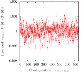 |
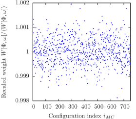 |
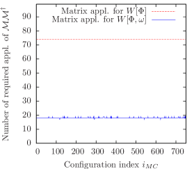 |
| (a) | (b) | (c) |
This is to be compared with the results obtained by the Krylov-space based reweighting strategy. In Fig. 5.8b the corresponding scaled weight factors calculated in the same Monte-Carlo run are presented. The latter weights are exact and do therefore not exhibit any statistical error. For clarification it is pointed out that the two presented weight factors are not supposed to coincide.
The numerical cost associated to the new reweighting scheme are presented in Fig. 5.8c and compared to those of the Gaussian estimation for one single sampling point. One clearly observes that the Krylov-space based method requires significantly less applications of the fermion operator than the Gaussian estimator. Here, a factor of about is observed. The lower numerical cost of the new reweighting technique and the fact that the latter approach is exact thus constitute the advantages of the Krylov-space based method.
In the given example the fluctuation of has been adjusted to be of the order . This can be done by an appropriate choice of the approximation interval and the degree of the approximation polynomial. A crude estimate of the expected fluctuation of can be given for the case where all eigenvalues of are contained within the approximation interval . Let be the corresponding orthonormal eigenvectors. After the direct sampling of the pseudo-fermion fields , which will be described in detail in section 5.5, one has
| (5.70) |
where the real and imaginary parts of the complex coefficients are random variables sampled according to a Gauss distribution with standard deviation of 1, i.e. . The weight factor is then given as
| (5.71) |
with
| (5.72) |
To roughly estimate the latter quantity we will assume here the eigenvalues to be independently and uniformly distributed within the interval . We further define the average relative deviation as
| (5.73) |
where the expression has been given in Eq. (5.10). Under the aforementioned assumptions the variance of , which is given as
| (5.74) |
then becomes
| (5.75) |
which can roughly be estimated as
| (5.76) |
when exploiting the relations and according to the above assumptions and considering the eigenvalues to be constant over the averaging procedure. One would thus expect the standard deviation of the logarithm , which is defined as
| (5.77) |
to be approximated by
| (5.78) |
Though this estimate is rather crude because all eigenvalues have been assumed to be independently distributed, the given estimate nevertheless turns out to describe the actual behaviour of the quantity as observed in direct Monte-Carlo calculations fairly well as can be seen in Tab. 5.5. For this listing the example Monte-Carlo runs that have already been considered several times before have been repeated with different setups of the underlying approximation polynomial.
The crucial question, however, is whether the numerical results on the physically relevant observables are actually independent of the choice of the approximation polynomial in a practical Monte-Carlo calculation. Moreover, it is important to ask how the resulting statistical uncertainty of the considered observables is affected by the reweighting strategy. For the purpose of clarification the average magnetization as well as the Higgs correlator mass , the numerical extraction method of which will be discussed in section 6.1.1, have been computed in the aforementioned series of Monte-Carlo calculations. The obtained results are presented in Tab. 5.5 and one finds that the considered observables, serving here as typical representatives for the observables of physical interest in this study, are indeed independent of the underlying approximation polynomial apart from statistical deviations of the size of the given error estimates, as expected.
Concerning the effect on the statistical uncertainty one finds for both considered observables, though most clearly noticeable for the average magnetization , that the latter uncertainty is not significantly affected by the the value of the relative deviations provided that is below a certain threshold value. Above that threshold, however, the statistical uncertainty of the considered observable rises quickly. The crossing of that threshold value occurs when the fluctuation of the weight factor becomes comparable to that of the considered, unweighted observable evaluated on the generated field configurations .
Choosing an optimal fluctuation scale is thus a trade-off between pure simulation speed, which is proportional to , and the statistical uncertainty of the considered expectation value increased by the fluctuations of the weight factor . In this work was typically chosen rather conservative, i.e. not larger than the fluctuation of the most stable considered observable, which is the magnetization for the most cases. Depending on the observables that one is mostly interested in, one can, however, exploit the relative independence of the underlying approximation polynomials to significantly increase the overall performance of the simulation algorithm in terms of achieved accuracy per numerical cost.
Finally, one may ask why the Krylov-space based method for computing has not directly been employed for constructing a simulation algorithm in the spirit of an HMC-algorithm, having simply the CG-solver replaced by the latter method. This would indeed be possible, if one succeeds in providing an efficient ansatz for calculating the molecular dynamics forces in such an approach.
It is further remarked that the here presented Krylov-space based, exact, and very efficient reweighting technique can immediately be applied also to the case of QCD.
| 8 | 2200 | 1.2497(239) | 0.1177(51) | ||||
| 10 | 2180 | 1.2515(49) | 0.1144(37) | ||||
| 12 | 2200 | 1.2512(25) | 0.1158(34) | ||||
| 14 | 2200 | 1.2541(15) | 0.1127(32) | ||||
| 16 | 2180 | 1.2497(16) | 0.1069(32) | ||||
| 18 | 21780 | 1.2506(5) | 0.1116(12) | ||||
| 8 | 2220 | 0.2019(31) | 0.4060(94) | ||||
| 10 | 2280 | 0.2024(21) | 0.4241(69) | ||||
| 12 | 2260 | 0.2021(3) | 0.4230(67) | ||||
| 14 | 2280 | 0.2019(6) | 0.4174(73) | ||||
| 16 | 22360 | 0.2025(1) | 0.4243(23) | ||||
5.5 Direct sampling of pseudo-fermion fields through polynomial approximation
The most efficient way for updating a field configuration in a Monte-Carlo process with respect to the auto-correlation would be its direct sampling according to the corresponding probability distribution, leading then to zero auto-correlation time. While this type of sampling is not feasible for the scalar field in the considered Higgs-Yukawa model except for the case of the free theory with , the pseudo-fermion fields , more precisely the transformed pseudo-fermion fields are Gaussian distributed according to Eq. (5.6) with the probability density , where the index runs from to . The standard idea for updating the pseudo-fermion fields is thus to sample the transformed fields according to the latter Gaussian distribution and to obtain from this sample through the inversion of the defining equation of according to
| (5.79) |
There are several ways to solve Eq. (5.79) for a given vector . A standard approach [151] applicable to QCD relies on the fact that the polynomial of the hermitian version of the QCD-Dirac operator can be written as the product
| (5.80) |
where is an explicitly constructable [151] polynomial that can be determined on the basis of the square roots of the roots of the polynomial . The pseudo-fermion fields are in this scenario not obtained from Eq. (5.79) but from
| (5.81) |
where the application of the inverse of the composed operator can be computed by means of a CG-algorithm.
It is remarked here that the latter computation is very well feasible in practice despite the large number of Dirac operator applications contained in the operator . The reason is that the number of necessary CG-iterations is typically of order [151], due to the operator exhibiting a very small condition number by construction, which results from the polynomial being an approximation of in this example. For other functions underlying the latter approximation the definition of the operator has to be adapted analogously to still guarantee its condition number to be small. The total numerical costs of the approach in Eq. (5.81) sum up to in terms of applications of . It should be noted that the condition number of depends on the accuracy of the approximation polynomial . The number of required CG-steps is thus expected to rise when one lowers the accuracy of the underlying polynomial.
For the case of the considered Higgs-Yukawa model, however, the approach given in Eq. (5.81) cannot directly be taken over. This is because there is no obvious way to decompose the polynomial according to Eq. (5.80) due to the lack of appropriate hermiticity properties of the fermion operator as discussed in section 3.6, which is in contrast to the above described situation in QCD. Therefore, a different approach for the direct sampling of the pseudo-fermion fields will be used.
Here, the idea is to compute Eq. (5.79) by means of a polynomial approximation for the function . The approximation interval for is chosen to be , starting explicitly at zero. This is possible since the function has no singularity in the interval . The degree of this approximation polynomial can be chosen sufficiently high such that its maximal relative deviation , which is defined analogously to Eq. (5.2), is of order of the machine precision. The pseudo-fermion fields are then directly obtainable through
| (5.82) |
In general, there are many ways to construct such an approximation polynomial for a given function to be approximated. The method described in section 5.1 could be adopted to the construction of an optimal approximation polynomial with respect to a minimal norm of the relative residual by defining an appropriate scalar product analogous to Eq. (5.9). Such an approach, however, would rely on the ability to calculate the aforementioned scalar product between the considered function and a chosen set of basis polynomials to very high precision in order to determine the polynomial coefficients reliably as discussed in section 5.1. This is straightforward for the case , since an explicit analytical expression for the considered scalar product can then trivially be derived. In the case considered here, however, the resulting integral expressions are more complicated hindering their obvious analytical solution. A numerical calculation of these expressions to the required numerical accuracy, on the other hand, would be extremely demanding with respect to the numerical costs.
A method for the construction of the approximation polynomial , that evaluates the function on a discrete, finite set of sample points only, is therefore favorable in this case. The standard Chebyshev approximation [127] is such a method. It determines the polynomial coefficients of with respect to the Chebyshev polynomial basis , i.e.
| (5.83) |
by explicitly solving the set of linear equations
| (5.84) |
with respect to the coefficients , where is a set of given sample points. In the standard Chebyshev approximation these sample points are chosen as
| (5.85) |
rendering the solution of Eq. (5.84) particularly simple by virtue of the orthogonal structure of the vectors given as with . It is well-known that the representation of in terms of Chebyshev polynomials then allows for a very stable evaluation of Eq. (5.82), since the numerically very stable recursion scheme
| (5.86) | |||||
| (5.87) | |||||
| (5.88) |
can be used for the evaluation of the Chebyshev polynomials [127]. It should be noted that the given form of the sample points in Eq. (5.85) as well as the recursion scheme assumes the Chebyshev polynomials to be defined on the interval . Adequate rescalings to adopt the given formulas to the here considered approximation interval are implicitly assumed in the following.
The described standard Chebyshev approximation is easily implementable and yields reasonably accurate approximation polynomials. Finding the optimal approximation polynomial for a given polynomial degree, however, requires a different algorithm, the well known Remez-algorithm [189, 127] for instance. It is an iterative procedure that generates a sequence of approximation polynomials . In each iteration step the polynomial is constructed from a given set of sample points by solving a set of linear equations. The sample points are then tuned by relocating them to the positions of the extrema of the residual . A common start constellation that typically yields good accuracy even without the aforementioned tuning is to choose the extrema of the Chebyshev polynomial as the start constellation.
The tuned Remez algorithm is thus the method of choice to obtain the most accurate approximation polynomial constructable for a given polynomial degree. Here, however, only the untuned version of the latter algorithm has been implemented, which already works satisfactorily for our purpose. Examples of the required polynomial degree to approximate the function to a specified accuracy are given in Tab. 5.6. Here, the targeted maximal relative deviation of the approximant has been set to and the presented parameters of the underlying polynomial have been taken from some actually performed lattice calculations as specified in Tab. 5.1 through the settings and . In this presentation the quantities and give the polynomial degrees required for the approximation polynomial as determined by the above described methods, i.e. the standard Chebyshev and the untuned Remez algorithm, respectively, to reach the aspired value of .
| 0.1 | ||
| 1.0 | 1.0 | |
| 18 | 220 | |
| 55 | 685 | |
| 54 | 677 | |
| 65 | 772 | |
| 102 | 1213 |
The key observation is that the direct sampling of the pseudo-fermion fields can indeed be performed quite efficiently by means of the considered polynomial based approach. One can infer from Tab. 5.6 that the numerical costs for this kind of direct sampling with a given setting of equals approximately three times the expenses of applying to a given pseudo fermion vector, at least in the considered examples. This should be compared to the would-be costs of the – here not applicable – sampling method given in Eq. (5.81), which sum up to in terms of applications of . The resulting would-be costs for the considered examples are also listed in Tab. 5.6 assuming the necessary number of CG-steps to be and , respectively, which clearly is a non-pessimistic assumption. This is especially true in the case where is not an absolute lower bound of the eigenvalue spectrum of the underlying fermion operator, since in that case the condition number of is no longer guaranteed to be of order .
It is finally remarked that this method should be further improvable by applying the fully tuned Remez algorithm to find the optimal approximant . Moreover, it is mentioned that the given approach for the direct sampling of the pseudo-fermion fields is directly applicable also to the case of QCD, provided that a PHMC algorithm is employed for its numerical evaluation.
5.6 Higher order multiple time-scale integrators
The concept of multiple time-scale integration schemes [190] is based on the observation that it is often possible to partition the total action into several contributions with
| (5.89) |
such that the corresponding forces acting on the conjugate momenta of the scalar field during the integration of the equation of motion differ strongly in strength and required computation time. Such a decomposition can then lead to a significant reduction of the overall numerical costs of performing the aforementioned molecular dynamics integration, provided that there is a correlation between the average strength of the forces and their numerical costs, such that the strongest forces require distinctly less computing resources for their calculation than the weaker ones. In this case the idea would be to construct a -times nested integration scheme with different nested integration step sizes , where longer step sizes would be assigned to the weaker, numerically more expensive forces while shorter step sizes would be used for the integration of the strong, rather inexpensive forces.
Using the same notation as in section 3.5 one can easily extend the leap-frog integration scheme given in Eq. (3.117-3.120) to its multiple time-scale version. For that purpose we define
| (5.90) |
The corresponding trajectory propagation operator for the given total trajectory length given as
| (5.91) |
where the Liouville operator has already been introduced in Eq. (3.110), can then again be approximated by using the Baker-Campbell-Hausdorff formula in Eq. (3.115) yielding
| (5.92) | |||||
| (5.93) |
with and denoting the number of integration steps for the nested integration on the -th time-scale. The total number of integration steps with respect to the force is thus given as . It is remarked that the symplecticity and reversibility properties of this nested leap-frog scheme are directly inherited from the single time-scale leap-frog scheme discussed in section 3.5.
The above presented nested leap-frog integration scheme can be further extended to a more general, higher order scheme by replacing Eq. (5.93) with
| (5.94) |
where the coefficients specify the integration scheme applied on the -th time scale and is the associated convergence order arising from this more general BCH-formula. For any desired order it is possible to select appropriate values for and , with such that the desired convergence order in Eq. (5.94) is achieved. Furthermore, it can additionally be requested that , , and , which would then automatically guarantee the reversibility of the resulting integration scheme. The symplecticity follows again from the fact that all operators in Eq. (5.94) have a determinant of one, as discussed in section 3.5. Examples for such sets of coefficients, taken from LABEL:Omelyan:2003zu, are provided in Tab. 5.7.
| LF | O2 | O4 | |
| 2 | 2 | 4 | |
| 2 | 3 | 6 | |
| 0.5 | 0.1931833275037836 | 0.08398315262876693 | |
| 1 | 0.5 | 0.2539785108410595 | |
| 0.5 | 0.6822365335719091 | ||
| 0 | 0.5 | -0.03230286765269967 | |
| – | 0.1931833275037836 | ||
| – | 0 | ||
| – | – | ||
| – | – | -0.03230286765269967 | |
| – | – | 0.6822365335719091 | |
| – | – | 0.2539785108410595 | |
| – | – | 0.08398315262876693 | |
| – | – | 0 |
In the actual implementation of the PHMC algorithm two higher order integration schemes have been included in addition to the standard leap-frog scheme. These are an order101010The subscript is dropped here and in the following when referring to the properties of the integrator in general, independent of the respective time-scale. and an order Omelyan integration scheme, the parameters of which are taken from LABEL:Omelyan:2003zu and listed in Tab. 5.7. These numerical schemes will be denoted as LF-, O2-, and O4-integrator, respectively, in the following. A particularity about the latter two Omelyan integrators implemented here is that the asymptotic number of required force evaluations111111’Asymptotic’ means here averaged over an infinite number of subsequent integration steps each of size . The underlying rationale is that the first force in an integration step equals the last force of the preceding integration step. for a single integration step of size , which is given by , is larger than it would minimally have to be to reach the specified order. In fact, the leap-frog scheme needs one force evaluation less than the O2-integrator but both schemes have the same convergence order . Furthermore, there are also order integrators specified in LABEL:Omelyan:2003zu which need less force evaluations than the considered O4-integrator. In fact, only three force evaluations are required to construct an order integrator. The arising additional freedom in the choice of the underlying parameters , is used in the presented more complex schemes to minimize the first non-vanishing coefficient in the -expansion of the residual appearing in Eq. (5.94). It could be shown that this numerical investment leads to an overall performance advantage of the Omelyan integrators over their unimproved counterparts with minimal nominal numbers of force evaluations by means of a higher acceptance rate [162].
The presented multiple time-scale integration scheme given in Eq. (5.94) shall now be applied to the case of the considered Higgs-Yukawa model. The main question is then how the total action should be partitioned into the contributions , such that the associated forces are either inexpensive or expensive but small compared to the other forces. An obvious idea is to separate the purely bosonic part of the action leading then to a two time-scale approach, i.e. , with the contributions
| (5.95) | |||||
| (5.96) |
where is the fermionic part of the total action as defined in Eq. (5.6). The outer integrator uses here a step size of to integrate the fermionic contribution , while the inner integrator applies the step size . Though it is not clear how strong the inner, purely bosonic force actually is in comparison to the outer force, i.e. the fermionic force, it is apparent that the numerical costs for the computation of are very low, making the presented approach thus a promising candidate for an overall reduction of the numerical expenses generated by the integration process.
An explicit example for the relative sizes of the considered forces is presented in Fig. 5.9. Here, the averaged total force in momentum space as given in Eq. (5.42) is presented versus the squared lattice momentum together with the corresponding measurements of the partitioned forces and , which are defined analogously. These results have been obtained in the Monte-Carlo run specified in Tab. 5.1 through the setting . One observes that the fermionic force is indeed significantly smaller than the bosonic contributions, except for the situation at small momenta. However, for the major fraction of momentum modes the aspired pronounced hierarchy of the considered forces is clearly observed, which is encouraging enough to investigate the actual benefit of the multiple time-scale integration scheme given in Eq. (5.94).
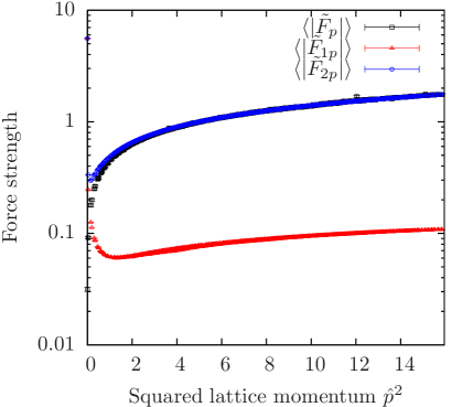 |
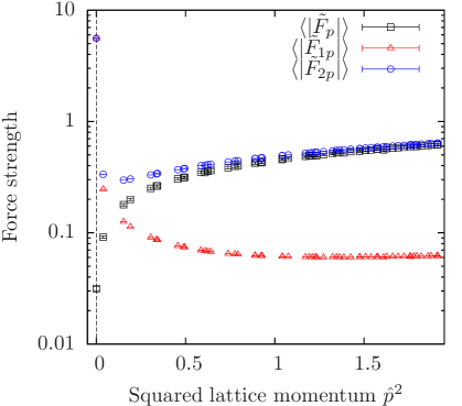 |
| (a) | (b) |
For that purpose a measure for the numerical cost of the underlying integration scheme has to be specified. In analogy to the cost measure given in Eq. (5.61) we define
| (5.97) |
where is the number of applications of the fermion operator required for the numerical integration from to and denotes the average acceptance rate. The latter cost measure has then been evaluated based on the aforementioned Monte-Carlo data and the obtained results are presented in Fig. 5.10a.
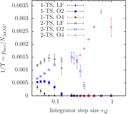 |
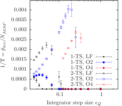 |
| (a) | (b) |
Before continuing with the discussion of the given numbers, however, the details of the determination of the specified cost measure shall be briefly discussed. It has been evaluated for various integration schemes and for different outer step sizes . This has been done outside the actual Markov process by taking the field configurations after their completed generation in the respective Monte-Carlo run as the common starting points for all considered integration schemes. All considered schemes were then applied on the same basis of underlying start field configurations, moreover, also with identical start values for the conjugate momenta as well as identical pseudo-fermion fields , which are both directly sampled as previously discussed. The observed differences in the acceptance rate are thus solely due to the properties of the integration scheme and are not induced by differences in the starting conditions. The value of the average acceptance rate was then determined by averaging over the observed variation , given as the difference between the values of at the beginning and at the end of the integration process, according to
| (5.98) |
For each considered integration scheme this experiment has been repeated for various settings of the steps size of the outer integrator.
In Fig. 5.10a the respective results of six different integration schemes are compared to each other. These are the LF-, the O2-, and the O4-scheme with only a single time-scale (1-TS), i.e. , and , as well as the nested LF-, O2-, and O4-schemes with (2-TS) and the partitioned forces chosen according to Eq. (5.95-5.96). In the latter case the specified scheme, being LF, O2, or O4, refers to the outer integrator, while the inner integration of the bosonic forces is always performed based on the setting , leading to a very accurate integration of the bosonic force contributions, such that the fermionic force is the main source for the observed variation .
With this background information at hand one can learn from Fig. 5.10a that the separation of the bosonic force onto a finer sampled time-scale indeed results in a substantial performance gain by a factor of approximately 6 in the considered example. One can also observe that the applied Omelyan O4-scheme is about 2 times more efficient than the other time-scale schemes considered in the investigated setup.
The latter observation concerning the performance differences between the LF-, O2- and O4-schemes, all of which applied with the same time-scale structure, depends, however, on the underlying model parameter setup. This is illustrated by an additional example given in Fig. 5.10b, showing the analogous results evaluated for a different Monte-Carlo run with infinite quartic coupling constant, i.e. . The detailed parameter setup underlying these results are specified in Tab. 5.1 through the setting . In this plot one still observes the superiority of the time-scale integrators over their single time-scale counterparts. The most efficient scheme is now, however, the O2-scheme exceeding the performance of the formerly optimal scheme by around in this example. Testing different integration schemes for a given set of model parameters can thus be worthwhile with respect to tuning the overall performance of the implemented algorithm.
Driven by the success of the considered multiple time-scale approach, the underlying technique for partitioning the forces shall be extended in the following, aiming at the further decomposition of the fermionic force . Here, we shall have in mind the situation of non-degenerate Yukawa coupling constants set to its phenomenological ratio. It has been discussed in section 5.2.2 that the condition number of the fermion operator becomes relatively large in that scenario leading then to the necessity of considering approximation polynomials of degree 200-300. It would thus be very desirable to have a means at hand with which also the fermionic force could be partitioned into numerically expensive, but weak, as well as strong, but inexpensive, forces.
For that purpose the fermionic part of the action is rewritten here as a telescope sum according to
| (5.99) | |||||
where the polynomials are approximation polynomials to the same function in our case. The polynomials differ only in their polynomial degree , their maximal relative deviation , and the lower bound of their respective approximation intervals , while the upper interval bound is identical for all polynomials. One can then decompose the total action into the contributions according to
| (5.100) | |||||
| (5.101) | |||||
| (5.102) |
It shall be remarked here, that no additional pseudo-fermion fields have been introduced in contrast to some other multiple time-scale approaches [191, 192]. Moreover, all techniques for applying the aforementioned polynomials of to a given vector as well as the techniques for calculating the respective fermion forces are directly inherited from what has already been discussed in section 5.1, since the difference of two polynomials is again a polynomial. The idea here is to use polynomials with very different degrees and relative accuracies, ordered according to their respective polynomial degree, such that . For an appropriate choice of these polynomials one can then expect to observe an ordering of the averaged force strengths according to , as required for a profitable application of the nested integration scheme presented in Eq. (5.92-5.94).
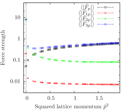 |
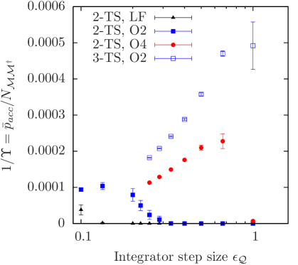 |
| (a) | (b) |
An example for the hierarchy of the force strengths is presented in Fig. 5.11a. Here, the presented force strengths have been obtained in the Monte-Carlo run specified in Tab. 5.1 through the setting . In this example, the action was split up into three parts, i.e. , according to Eq. (5.100-5.102). The two underlying polynomials and have been chosen to have the very distinct degrees and . Also the values of the lower approximation interval bound differ strongly. Here we have and . In the presented plot one clearly observes a very pronounced separation of the force strengths associated to the partitions . Here, the strongest force is produced by the most inexpensive contribution, i.e. the bosonic contribution , followed by the remaining two forces and in ascending order with respect to their numerical costs, as aspired. Again this observation only holds at sufficiently large momenta. For the major part of the momenta, however, the considered forces are clearly separated by a factor of approximately one order of magnitude, thus rendering the presented force partitioning a promising candidate for the intended performance improvement.
The actually obtained performance of this time-scale (3-TS) integration scheme is presented in Fig. 5.11b. Here, the parameters of the outer integrator have been chosen according to Tab. 5.7 as specified through , i.e. the outer integrator is given here as the O2-scheme. The two inner integrators have been configured with , and , . The resulting inverse costs are then presented versus the varying value of the outer step size . These results are compared to the time-scale LF-, O2-, and O4-schemes as already considered above. The latter are based, of course, on the finer polynomial with degree . One clearly observes significant differences between the presented schemes with respect to the measure . In particular, one sees that even the best considered setup for the time-scale approach, which was found to be far superior to the single time-scale schemes discussed above, can be beaten by the presented time-scale scheme improving the numerical performance by a factor of approximately 2.
It is finally remarked, that the presented approach of splitting up the fermion action in terms of a telescope sum according to Eq. (5.99), yielding then several fermion forces with potentially very different force strengths, can directly be applied also to the case of QCD, provided that a PHMC algorithm is employed for its numerical evaluation.
Chapter 6 Results on the lower Higgs boson mass bound
The simulation algorithm detailed in the previous chapter shall now be applied to the actual determination of the lower Higgs boson mass bounds. Before such mass bounds can be derived, however, a certain amount of preparation work has to be invested to build up the basis for the eventually intended calculations. First of all, the so far unspecified details of the Higgs boson mass determination have to be clarified. This will be discussed in section 6.1 together with the extraction method for the Goldstone renormalization constant and the fermion mass computation.
In a next step some analytical formulas for the dependence of the vacuum expectation value , the Higgs boson self-energy, and the quark masses on the model parameters will be derived from lattice perturbation theory (LPT) in section 6.2. The observed good agreement between these analytical predictions and the corresponding numerical results obtained in direct Monte-Carlo calculations can be understood as an indication for the correctness of the implemented simulation algorithm. The analytical predictions on the quark masses will later also be helpful to understand the finally observed dependence of the numerically obtained quark masses on the cutoff and the lattice volume.
In section 6.3, the Higgs boson mass will alternatively also be estimated by calculating the effective potential introduced in section 4.1.1. Here, however, the already given result on the effective potential is extended by incorporating the missing contributions, allowing then to study the Higgs boson mass dependence on the model parameters , , and , in particular. From the obtained results it will be concluded that the lowest Higgs boson mass is indeed obtained at vanishing bare quartic coupling constant as one would have expected from the qualitative result in Eq. (3.83).
With this preparation at hand the lower Higgs boson mass bounds can eventually be established by evaluating the Higgs boson masses attainable at with the Yukawa coupling constants adjusted such that the phenomenologically known values of the quark masses are reproduced. This will be done in section 6.4.1 for the degenerate scenario with equal top and bottom quark masses, which is numerically fairly well accessible and moreover conceptually well under control. This situation changes when proceeding to the lower Higgs boson mass bound determination in the physically more relevant setup with and tuned to its phenomenological value, as discussed in section 6.4.2.
Finally, the question for the universality of the obtained Higgs boson mass bounds will be addressed in section 6.5, where the model will be extended by some higher order self-interaction terms of the scalar field. Such an extension is not excluded by the usual renormalization arguments, since the Higgs-Yukawa sector can only be considered as a trivial theory with a non-removable cutoff by virtue of its triviality property. The effect of these additional coupling terms on the attainable Higgs boson masses is then investigated and it is found that the previously established lower mass bound can indeed significantly be altered.
6.1 Details of the particle mass determination
The so far unspecified details concerning the computation of the physical observables defined in section 3.4 shall now be given in the subsequent sections. We will begin with the discussion of the Higgs boson mass determination based on the Higgs time-slice correlator in section 6.1.1, since this will be the method of choice in the weakly interacting regime of the considered Higgs-Yukawa model. The reasoning is that this approach does not rely on any analytical continuation of Euclidean results to Minkowski space-time and does therefore not suffer from the systematic uncertainties connected to such an analytical continuation in contrast to the mass determination based on the Higgs propagator analysis as proposed in section 3.4. This approach is justified as long as the Higgs boson can be treated as a stable particle, which seems acceptable in the weakly interacting regime of the considered model, as discussed in section 2.2, allowing then for a straightforward determination of the Higgs boson mass by studying the decay properties of the Higgs time-slice correlator .
The methods for the extraction of the Goldstone renormalization factor and the Higgs boson masses , based on the analysis of the respective propagators are then presented in sections 6.1.2 and 6.1.3. Finally, the fermion mass determination is discussed in section 6.1.4.
The applicability of all presented computation schemes will be demonstrated for the selected Monte-Carlo runs specified in Tab. 6.1. The listed lattice calculations, serving here as typical examples for the weakly interacting regime of the considered model, have been chosen to cover the full range of cutoffs that will be investigated in the remainder of this chapter.
6.1.1 Analysis of the Higgs time-slice correlator
The Higgs correlator mass was defined in Eq. (3.74) via the exponential decay of the Higgs correlation function at large time separations . Provided that the Higgs boson can be considered as a stable particle, meaning here that contributions to the correlation function arising from lighter energy eigenstates of the underlying Hamiltonian are negligible, the determined correlator mass coincides with the physical pole mass given by the pole of the Higgs propagator, as discussed in section 3.4.
In the context of the considered Higgs-Yukawa model, however, this condition is only approximately fulfilled even in the weakly interacting region of the parameter space. In fact, one would expect the massless Goldstone modes to contaminate the correlation function . More precisely, it is not the single Goldstone modes that mix into but the two Goldstone states, which have the same quantum numbers as the Higgs boson. The single Goldstone modes are distinguishable from the Higgs modes by their isospin and are thus projected out by the operator underlying the Higgs time-slice correlation function as defined in Eq. (3.73). The idea here is to respect the contribution arising from the almost massless two Goldstone states by choosing an appropriate fit ansatz for the correlation function . Though it is well-known that on a finite lattice volume the Goldstone particles are not exactly massless [149], the contamination induced by these states is here accounted for by incorporating an additional constant term into the fit ansatz according to
| (6.1) |
where , , and denote the free fit parameters. Moreover, the fit is assumed to be performed at sufficiently large values of to avoid a contamination by excited states. This simple form is chosen here for the sake of the stability of the fit procedure. Additionally, the less flexible and thus even more stable fit approach
| (6.2) |
will also be applied to fit the Higgs correlation function . In this latter ansatz the constant term has been neglected making this ansatz insensitive to possible contaminations arising from lighter states on the one hand, but more stable on the other hand. The motivation for this second approach lies in the assumption that the contributions of the lighter two Goldstone states to the correlation function might be negligible from a practical point of view in the weakly interacting regime of the considered model. In the following both approaches will therefore be applied and compared to each other.
The alert reader, however, may wonder whether the mass extraction based on the analysis of the long ranged decay properties of the correlation function is justified at all, since this latter function is constructed from the operator , which is non-local in time. This non-locality arises from the rotation of the field introduced in section 3.3 yielding the rotated field which actually underlies the latter operator . By virtue of this rotation the usual arguments of the transfer matrix formalism can thus not directly be applied to the aforementioned operator in the standard manner, as presented in Eq. (2.2), to establish the connection between the long range behaviour of the correlator and the particle mass spectrum. The correlation function associated to the rotated field has therefore explicitly been studied in the framework of the pure -theory [124]. It was found that the operator , though non-local in time, still leads to an exponentially decaying correlation function , allowing for the determination of the Higgs boson mass in the above described manner, with the downside, however, that the obtained Higgs boson mass is contaminated with additional finite volume contributions.
For the purpose of testing these findings also in the broader context of the considered Higgs-Yukawa model an alternative Higgs time-slice correlation function is defined here based on the local operator
| (6.3) |
according to
| (6.4) |
where an adequate modulo operation is implicit to guarantee .
The given operator determines the direction of the Higgs mode in terms of the components of the field on each time-slice separately and is thus local in time. The transfer matrix formalism is therefore directly applicable to the corresponding correlation function in the standard manner. The above described procedure for extracting the Higgs boson mass from the correlation function can thus be applied to without the aforementioned conceptual difficulties. The same fit formulas already given in Eq. (6.1) and Eq. (6.2) will therefore also be applied to .
Examples for the correlation functions and obtained from the direct Monte-Carlo calculations specified in Tab. 6.1 are presented in Fig. 6.1a,d. These plots also show the respective fits resulting from the approaches given in Eq. (6.1) and Eq. (6.2).
The other four plots in Fig. 6.1 show the effective correlator masses obtained from the two different correlation functions and combined with the two given fit functions. The effective masses are implicitly defined through
| (6.5) |
and can easily be computed by solving the given equation numerically. Here the symbol stands either for the correlation function or and is the fit parameter of Eq. (6.1) or zero if the fit ansatz in Eq. (6.2) is used.
The effective masses are supposed to decrease monotonically with rising and to converge to a plateau value for sufficiently large values of , which gives the actual correlator mass according to its definition in Eq. (3.74). Since the statistical error of the effective masses generally grows with increasing , the choice of the value of where to read off the result for the Higgs boson mass is a trade-off between systematic and statistical uncertainties. To determine one would usually fit to a constant within a window of starting at a value where the plateau building has already set in.
Here, however, the statistical errors of the effective masses are very large compared to the effect induced by the contamination of the correlation functions through excited states. A reliable distinction between a phase of monotonic decrease of and the onset of a plateau building is thus not very practical here. In the following the Higgs boson mass will therefore not be determined by the effective masses themselves but through the overall cosh-fits given in Eq. (6.1) and Eq. (6.2). The Higgs boson masses resulting from these fits are compared to the respective effective masses in Fig. 6.1. Although the presented correlator masses have even been obtained by fitting the Higgs correlator over the full range of , one finds that the obtained results on are perfectly consistent with the corresponding effective masses, thus justifying the chosen method of determining the correlator masses.
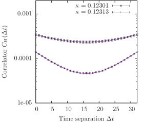 |
 |
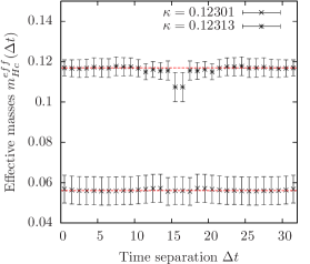 |
| (a) | (b) | (c) |
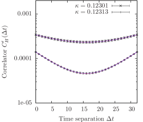 |
 |
 |
| (d) | (e) | (f) |
The resulting Higgs correlator masses determined in the described manner are listed in Tab. 6.2. One learns from these findings that the mass obtained from the non-local operator and the local operator coincide within the error bars here. From this observation it is concluded that it is indeed justified to extract the Higgs boson mass from the correlation function associated to the non-local operator as originally proposed in section 3.4 at least in the weakly interacting regime of the considered model.
| Correlator | from | from | |
|---|---|---|---|
| 0.056(7) | 0.058(2) | ||
| 0.058(7) | 0.058(2) | ||
| 0.117(4) | 0.111(2) | ||
| 0.117(4) | 0.111(2) |
Furthermore, one sees in Tab. 6.2 that the masses obtained from the fit approach in Eq. (6.1), which accounts for contributions of massless states, seem to be somewhat larger than those determined by Eq. (6.2), if at all distinguishable with respect to the given statistical uncertainties. This is what one would have expected. However, the first approach is much more unstable than the second ansatz which is manifest in the larger statistical uncertainty of the corresponding results. Moreover, for the most cases the correlator masses determined with and without including a constant term into the fit ansatz have turned out to be not clearly distinguishable in practice with respect to the given errors.
One can therefore conjecture that it is favourable to use the less flexible fitting procedure in Eq. (6.2) to extract the Higgs boson mass from the correlation function due to the better stability properties of that ansatz. Furthermore, we will use as the underlying correlation function in the following. This is the approach that will be applied for the rest of this chapter.
6.1.2 Analysis of the Goldstone propagator
The Goldstone renormalization constant is required for determining the renormalized vacuum expectation value of the scalar field . It is thus needed for the fixation of the physical scale of a given Monte-Carlo run according to Eq. (3.58). This renormalization constant has been defined in Eq. (3.67) through a derivative of the inverse Goldstone propagator. As already pointed out in section 3.4 computing this derivative requires an analytical continuation of the discrete lattice propagator, which was proposed to be obtained via a fit of the discrete lattice data.

The idea here is to construct an appropriate fit function based on a perturbative calculation of the Goldstone propagator in continuous Euclidean space-time. For simplicity the consideration is again restricted to the pure -theory. To one-loop order the only momentum dependent contribution to the Goldstone propagator is given by the mixed Higgs-Goldstone loop illustrated on the right-hand side of Fig. 6.2. Adopting the same steps as detailed in section 2.2 to the case of the considered Higgs-Goldstone loop, one can establish the result for the renormalized Goldstone propagator at one-loop order yielding
| (6.6) |
where the one-loop contribution is given as
| (6.8) |
The different structure of the one-loop contribution as compared to the corresponding result for the pure Higgs loop contribution given in Eq. (2.31) is caused by the mixture of the different masses and appearing in the mixed Higgs-Goldstone loop illustrated in Fig. 6.2. For equal Higgs and Goldstone masses, i.e. , the given expression for the loop contribution recovers the result for the pure Higgs loop , as expected. For the given formula can moreover be shown to be finite111More precisely, the given function converges to a finite constant in the limit . at , as desired.
In principle one can directly employ the expression in Eq. (6.6) as the sought-after fit function . For clarification it is remarked at this point that instead of fitting the lattice propagator itself with , it is always the inverse propagator that is fitted with in the following. However, for the actual fit procedure of the lattice data a modified version of Eq. (6.6) is used given as222According to the symmetries of Eq. (6.9) one has , where appropriate mappings are implicitly assumed. This type of shorthand notation will extensively be used in the following.
| (6.9) |
where , , , and are the free fit parameters. Two modifications have been applied here to the original result. Firstly, the constant term in Eq. (6.6) has been replaced by simply for convenience. These changes are nothing but a reparametrization of the fit parameters, which is the reason why the masses and are not denoted here as the Higgs and Goldstone boson masses and , respectively. Strictly speaking, the different appearances of in Eq. (6.9) now refer to slightly different numbers in this reparametrization which are, however, identified here with each other for the sake of stability. Since the Goldstone mass is close to zero anyhow, this simplification is insignificant for a practical fit procedure. For clarification it is pointed out that in the here presented approach the Goldstone mass is actually not determined through the nominal value of the latter fit parameter itself, but through the pole of the resulting analytical continuation according to Eq. (3.66).
More interestingly, however, a global factor has been introduced in the denominator of Eq. (6.9) in the spirit of renormalization constant. This modification is purely heuristic and its sole purpose is to provide an effective description of the observed propagator, which is all we need at this point. It can, however, physically be motivated. For that purpose it is recalled that the given analytical result for the Goldstone propagator in Eq. (6.6) has been derived for the pure -theory only. In the following, however, the given fit ansatz will be applied to the full Higgs-Yukawa sector, including contributions from fermions. These fermionic contributions will influence the overall slope of the propagator in addition to the effect of the already accounted Higgs-Goldstone loop. It will also change the Goldstone mass itself, but such a shift is already covered by the fit parameter . The intention of the factor is thus to make the given ansatz sufficiently flexible to allow for its application also in the presence of fermionic contributions to the Goldstone propagator.
The alert reader may wonder, whether one should rather construct a fit ansatz from the renormalized result of the Goldstone propagator derived in the full Higgs-Yukawa sector. This would indeed place the fit procedure on an even better conceptual footing. However, it will turn out, that the given ansatz already works satisfactorily well for our purpose.
More important seems to be the question what part of the lattice Goldstone propagator should actually be included into the fit procedure. It was already pointed out in section 3.4 that the consideration of the lattice propagator has to be restricted to small lattice momenta in order to suppress contaminations arising from discretization effects. For that purpose the constant was introduced specifying the set of momenta underlying the fit approach according to . In principle, one would want to choose as small as possible. In practice, however, the fit procedure becomes increasingly unstable when lowering the value of . In the following examples we will consider the settings , , and . To make the discretization effects associated to these not particularly small values of less prominent in the intended fit procedure, the inverse lattice propagator is fitted with instead of , being a function of the squared lattice momentum , which is completely justified in the limit .
 |
 |
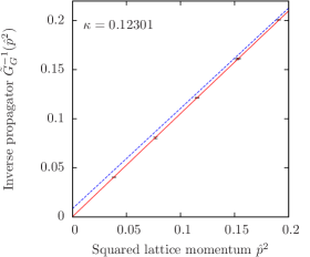 |
| (a) | (b) | (c) |
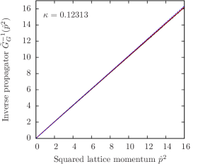 |
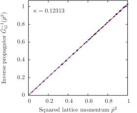 |
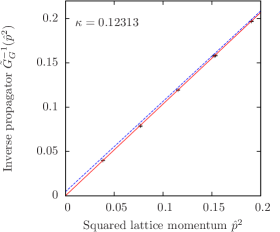 |
| (d) | (e) | (f) |
Examples of the given fit procedure are presented in Fig. 6.3 where the inverse lattice Goldstone propagators as obtained in the Monte-Carlo runs specified in Tab. 6.1 are shown together with their respective fits according to Eq. (6.9). For a clearer demonstration of the quality of the applied fit ansatz the presented numerical data are also compared to the linear fit function
| (6.10) |
where and are the only free fit parameters. One learns already from this graphical comparison that the linear fit ansatz is not suited for an adequate description of the Goldstone propagator at small momenta due to its pronounced curvature, being clearly observable thanks to the very small statistical errors of the lattice data. This becomes even more apparent when one considers the corresponding values of the average squared residual per degree of freedom listed in Tab. 6.3. While this quantity is close to its expected value of one for the fit ansatz , moreover approximately independent of the chosen value of as desired, the corresponding result associated to the application of the linear fit approach is much larger and rises clearly with increasing values of .
| fit ansatz | linear fit ansatz | ||||||
| 0.9641(37) | 0.000(1) | 0.71 | 0.9655(4) | 0.048(2) | 2.94 | ||
| 0.9654(45) | 0.000(1) | 0.92 | 0.9720(2) | 0.067(1) | 5.22 | ||
| 0.9699(17) | 0.010(18) | 0.95 | 0.9781(1) | 0.090(1) | 6 94 | ||
| 0.9722(140) | 0.000(1) | 0.90 | 0.9717(4) | 0.027(3) | 1.25 | ||
| 0.9775(44) | 0.000(3) | 0.91 | 0.9754(2) | 0.045(1) | 2.44 | ||
| 0.9784(65) | 0.004(10) | 1.09 | 0.9796(1) | 0.066(1) | 4.01 | ||
The Goldstone mass and the respective renormalization factor can then be obtained according to Eq. (3.66) and Eq. (3.67) from the analytical continuation of the lattice Goldstone propagator given by and , respectively. The results corresponding to the various settings of are listed in Tab. 6.3. While the statistical errors associated to the numbers obtained from the linear fit ansatz seem to be clearly favourable in comparison to the findings derived from the fit ansatz , the results arising from the linear ansatz are inconsistent for the different settings of . Especially the obtained Goldstone mass depends significantly on the chosen fit interval specified by the value of . The linear fit ansatz can thus not be applied for a reliable determination of the aforementioned Goldstone propagator properties.
This is in contrast to the situation of the more elaborate fit ansatz . All results derived by applying this latter approach are consistent with respect to the given errors. This observed freedom in the choice of will be used to select the rather large setting for the determination of the Goldstone renormalization constant in the later lattice calculations. The reason is that the given fit ansatz tends to become somewhat unstable on small lattices with low statistics and small values of . Choosing then allows for an unique approach applicable to all considered lattice calculations.
6.1.3 Analysis of the Higgs propagator
We now turn to the analysis of the lattice Higgs propagator. In principle we will follow the same steps already discussed in the preceding section. Again the idea is to determine an analytical continuation of the lattice propagator by fitting the latter to some adequate fit function . In section 2.2 we have already derived the perturbative one-loop result for the Higgs propagator of the pure -theory in continuous Euclidean space-time. Here, we will construct the sought-after fit function based on that earlier result given in Eq. (2.2).
However, with the same motivation already discussed for the case of the Goldstone propagator in the preceding section the original result in Eq. (2.2) is slightly modified, leading then to the fit function333Again the inverse lattice propagator will be fitted with the inverse expression instead of fitting with .
| (6.11) |
with the free fit parameters , , , and . One of the aforementioned modifications is that the constants and are given here as the loop contributions and evaluated at the origin instead of the location of the pole according to
| (6.12) | |||||
| (6.13) |
which simplifies the practical fit procedure. Consequently, the explicit appearance of the imaginary contribution in Eq. (2.2) is exactly canceled. These changes are nothing but a reparametrization of the fit parameters, which is the reason why the mass is not denoted here as the Higgs boson mass . The only real discrepancy between the fit ansatz given in Eq. (6.11) and the original perturbative result in Eq. (2.2), except for the introduction of the overall factor , is that the two appearances of the parameter in Eq. (6.11) would actually refer to two different parameters in this setup. For the sake of stability, however, these two parameters have been identified with each other here and are jointly referred to as .
The other modification is the introduction of the additional fit parameter which enters the given formula in Eq. (6.11) in the spirit of a renormalization constant. Again this modification is purely heuristic with the intention to provide an effective description of the observed propagator. The motivation for its introduction is the same as for the case of the previously discussed Goldstone propagator.
Examples for the quality of the specified fit approach are shown in Fig. 6.4. Here the given fit function was applied to the numerical lattice Higgs propagator calculated in the Monte-Carlo runs listed in Tab. 6.1. Following the same rationale given in the preceding section the inverse lattice propagators are actually fitted with , being a function of the squared lattice momentum . In the presented plots the threshold value for the fit interval was set to , which is a reasonable choice as discussed below, and one finds the performed fit to describe the numerical data very well. In addition, the obtained fit is compared to the naive ansatz of a linear fit approach given as
| (6.14) |
which is also presented in Fig. 6.4. In contrast to the preceding section, the linear fit also provides a very good description of the numerical data, which is due to the threshold value being chosen much smaller here than for the analysis of the Goldstone propagator. However, when one considers the corresponding average squared residuals per degree of freedom listed in Tab. 6.4 for a sequence of several different values of the parameter one learns that the more elaborate fit ansatz in Eq. (6.11) yields significantly better fit curves than , as the threshold value is increased.
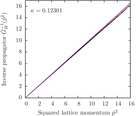 |
 |
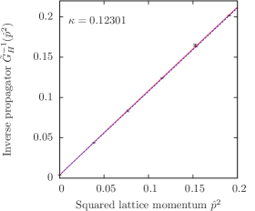 |
| (a) | (b) | (c) |
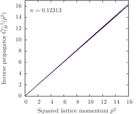 |
 |
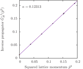 |
| (d) | (e) | (f) |
The Higgs propagator mass defined in Eq. (3.68) and the Higgs pole mass together with its associated decay width given by the pole of the propagator on the second Riemann sheet according to Eq. (3.66) can then be obtained by defining the analytical continuation of the lattice propagator as and , respectively. The results corresponding to the various performed fit procedures are listed in Tab. 6.4. Since the linear function can not exhibit a branch cut structure, however, the pole mass equals the propagator mass and the decay width is identical to zero for this linear fit approach. That is the reason why only the mass is specified in the latter scenario.
| Fit ansatz | Fit ansatz | |||||||
|---|---|---|---|---|---|---|---|---|
| 0.12301 | 1.0 | 0.058(2) | 0.056(2) | 0.056(2) | 0.000(0) | 1.26 | 0.062(2) | 2.01 |
| 0.12301 | 2.0 | 0.058(2) | 0.055(1) | 0.055(1) | 0.000(0) | 1.39 | 0.068(2) | 3.24 |
| 0.12301 | 4.0 | 0.058(2) | 0.052(1) | 0.052(1) | 0.000(0) | 1.56 | 0.080(3) | 4.05 |
| 0.12313 | 1.0 | 0.111(2) | 0.114(1) | 0.114(1) | 0.001(1) | 1.01 | 0.113(1) | 1.03 |
| 0.12313 | 2.0 | 0.111(2) | 0.110(1) | 0.110(1) | 0.000(6) | 1.07 | 0.116(1) | 1.27 |
| 0.12313 | 4.0 | 0.111(2) | 0.106(1) | 0.106(1) | 0.000(0) | 1.12 | 0.122(1) | 1.68 |
From the presented results one learns that the pole and propagator masses and obtained from the more sophisticated fit ansatz agree satisfactorily well with each other at and , where they are also consistent with corresponding value of the Higgs boson correlator mass that has been discussed in section 6.1.1. At the largest here presented threshold value, i.e. , the latter results deviate significantly from the aforementioned numbers making obvious the fact, that the threshold value has to be chosen sufficiently small to obtain reliable results for the sought-after propagator properties. Comparing the two different fit approaches, however, one finds that the more elaborate ansatz yields more stable fit results than the simple linear approach as the threshold value is varied at least for the presented example with the smaller hopping parameter. It is remarked at this point that the observed differences between the latter two fit procedures are in fact rather mild in the here considered scenario of small bare coupling constants. They will, however, become much more pronounced in the strongly interacting regime of the model as discussed in section 7.1.2.
Though the Higgs boson mass will actually not be determined by directly analyzing the Higgs propagator in the subsequent investigation of the lower mass bounds, but rather by studying the time-slice correlation function as detailed before, it is nevertheless concluded from the numbers presented in Tab. 6.4 that selecting the threshold value to be would be a reasonable choice for the final evaluation of the propagator properties, as already assumed in Fig. 6.4.
It is remarked that the conceptual footing of the applied fit approach could be further improved by including also the fermion contributions. However, from the above findings one can conjecture that the applied fit ansatz, albeit derived from the pure -theory only, already provides a sufficient means for determining the Higgs propagator and pole masses in a consistent manner, at least in the here considered weakly interacting regime of the Higgs-Yukawa model.
In principle, the chosen fit approach also allows to access the decay width according to Eq. (3.66) by numerically searching the pole of the analytically continued Higgs propagator on the second Riemann sheet. The resulting findings for are also listed in Tab. 6.4. It is remarked at this point that the latter numbers are very sensitive to small variations in the fit procedure due to the relative large number of free fit parameters considered here. However, all obtained numbers are fully consistent with zero within the given errors, which is in reassuring agreement with the assumption that the Higgs boson can be treated as a stable particle in the weakly interacting regime of the considered model.
6.1.4 Analysis of the fermion time-slice correlator
The fermionic time-slice correlation function has been defined in Eq. (3.75) and it has already been pointed out that the given correlation function would be identical to zero due to the symmetries of the considered model if it was evaluated in the background of the unrotated scalar field . The fermionic correlator is therefore computed after rotating the field as described in section 3.4, i.e. in the background of . As an example the top quark correlation functions , obtained in the lattice calculations specified in Tab. 6.1, are presented in Fig. 6.5a. The corresponding bottom quark correlators are not shown, since they yield identical results up to statistical fluctuations in the here considered mass degenerate setup. As already remarked in section 3.4 the full all-to-all correlator can trivially be computed, explaining the low statistical uncertainties of the given results.
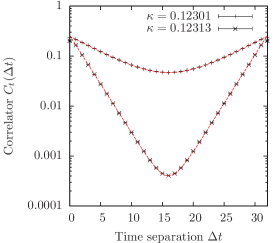 |
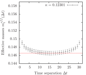 |
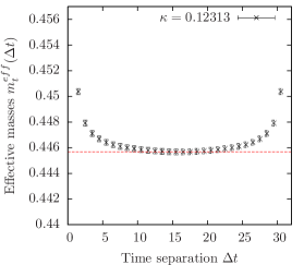 |
| (a) | (b) | (c) |
The presented lattice correlation functions have been fitted with the fit approach
| (6.15) |
which, however, was done here only for the purpose of illustration. The fermionic mass , as specified in Eq. (3.81), is actually determined by means of the effective fermion masses according to
| (6.16) |
where the effective masses are again defined implicitly through
| (6.17) |
Here, no constant term has been included in contrast to the corresponding definition of the bosonic effective masses given in Eq. (6.5), since the considered fermions are stable particles in the framework of the considered Higgs-Yukawa model, at least in the mass degenerate case with equal top and bottom Yukawa coupling constants.
The effective masses corresponding to the presented correlation functions are shown in Fig. 6.5b,c. Contrary to the case of the Higgs correlation function discussed in section 6.1.1 the obtained effective top quark masses are very accurate and allow for a clear observation of their expected monotonic decline with rising values of . The fermion masses can thus reliably be determined according to Eq. (6.16). This is the approach that will be used for the rest of this work.
6.2 Predictions from Lattice Perturbation Theory
In this section the basic concepts of lattice perturbation theory (LPT) in the context of the considered Higgs-Yukawa model will be briefly introduced. The resulting apparatus will then be applied in the following to derive analytical predictions for the symmetric-broken phase transition, the Higgs boson self energy, as well as the top and bottom quark masses.
It shall be remarked at this point that we will mostly use bare perturbation theory throughout this section. For our purpose of testing the lattice results which are obtained from a regularized theory with accessible, bare quantities, namely the model parameters , , and , this is the method of choice, provided that the corresponding perturbative series in the bare quantities converge sufficiently fast. It will turn out that this is indeed mostly444A counterexample will be presented in section 6.2.3. the case with respect to our needs, at least in the weakly coupling regime of the model at the considered values of the cutoff .
The main concept of the here considered approach is to split up the total action with its constituents defined in Eq. (2.49) and Eq. (3.26) into a Gaussian integrable part and an interacting part . The idea is then to expand the exponential of the interacting contribution into a power series in terms of , the summands of which can then be integrated with respect to the remaining weight according to
| (6.18) |
where is some considered observable.
The choice of how to split up the total action into a Gaussian part and the remainder , however, is not unique. In principle, this choice will not effect the final result of any calculation performed in such a perturbative expansion, provided that all terms of the summation in Eq. (6.18) are respected. Especially, no apriori knowledge about spontaneous symmetry breaking would then be needed and one could always expand the total action around the origin, i.e. around . In practice, however, the infinite sum in Eq. (6.18) is truncated after a few considered orders. The corresponding result in such a practical calculation will thus strongly depend on the chosen expansion point, i.e. on the chosen division of the total action into and . In case of a broken vacuum, for instance, the naive approach of expanding the total action around the origin, i.e. , would lead to very bad convergence properties of the associated perturbative series. For this case, which we will restrict the consideration to, it would be more appropriate to expand the total action around the non-vanishing vev , which we - at this point - assume to be given. It will later be determined self-consistently.
Using the definitions of the Higgs and Goldstone modes given in Eq. (3.57) the total action can now be expanded around the non-vanishing vev by dividing into the Gaussian-integrable part and the interaction parts according to
| (6.19) | |||||
| (6.20) | |||||
where the continuum notation of the lattice action in terms of the bare mass , the coupling constants and was used here for convenience, which are, however, trivially related to the lattice parameters , , and as discussed in section 3.3. Moreover, it is remarked that the summation over the fermion generations is implicit in this notation and that the symmetry of the model has been exploited allowing to assume the vacuum expectation value of the scalar field to point into the 0-direction. The so far unspecified expression and its momentum space representation are furthermore defined as
| (6.21) | |||||
| (6.22) | |||||
| (6.23) | |||||
| (6.24) |
where the underlying expression for , , and have been given in Eq. (4.20), Eq. (4.21), and Eq. (4.22), respectively.
The expectation value of a considered observable in the original theory can now be expressed as the expectation value with respect to the Gaussian action reweighted by the exponential of the interacting contribution according to
| (6.25) |
where the expectation value with respect to is defined as
| (6.26) |
with
| (6.27) |
In this notation the weight factor gives rise to the perturbative expansion in terms of the coupling constants , , and by virtue of its power series representation in Eq. (6.18). Since the action is Gaussian, all field variables appearing in the expansion of are statistically independent with respect to the statistical weight induced by . Moreover, the standard Wick theorem holds and all expectation values with respect to of odd powers of field variables vanish. The basic building blocks of this perturbative expansion are thus the bare, tree-level propagators generated by the Gaussian contribution . In momentum space they read
| (6.28) | |||||
| (6.29) | |||||
| (6.30) |
where the Higgs-, Goldstone-, and quark fields in momentum space are given as
| (6.31) | |||||
| (6.32) |
Furthermore, the structure of the interacting contribution in terms of the field variables in momentum space will be needed in the upcoming perturbative calculations. It is directly obtained from Eq. (6.20) and Eq. (6.31-6.32) yielding
Finally, it is remarked here that Eq. (6.28-6.29) only hold if the expansion point, which was chosen here to be the vacuum expectation value , is chosen large enough to guarantee the positivity of the corresponding denominators. Also Eq. (6.30) requires the expansion point to be non-zero. These requirements, however, are met when investigating the broken phase, as aspired.
6.2.1 Phase diagram from one-loop LPT
The apparatus introduced in the previous section shall now be applied to the calculation of the phase transition surface between the symmetric and the broken phase. More precisely, we will determine the dependence of the vev on the model parameters within the broken phase from one-loop lattice perturbation theory. The phase transition surface could then be obtained from these results in the same manner already described in section 4.1.2, if desired.
The main observation underlying the following calculation is that the total action could also have been expanded around the expansion point instead of the actual vacuum expectation value leading then to the same expressions already given in Eq. (6.19-6.20) with the only difference that the field would now be given as the fluctuation of around the expansion point . The scalar field would then no longer have the interpretation of being the Higgs field and its expectation value would not be zero. In fact, the expectation value of the zero momentum component vanishes if and only if the expansion point coincides with the true vacuum expectation value . More precisely, one has
| (6.34) |
The idea here is to calculate the expectation value in lattice perturbation theory for a given expansion point . The true vacuum expectation value can then be determined in this perturbative approach by identifying that value of the expansion point , where one finds .
In the following we will compute the expression to one-loop order. The resulting equation can then be solved numerically. Beginning with an arbitrary non-zero start value for the expansion point one can, for instance, iteratively define the sequence , through the iterative relation
| (6.35) |
where denotes the LPT result for given the expansion point . The fix-point of Eq. (6.35) would then give a self-consistent determination of the vacuum expectation value based on lattice perturbation theory.

The missing step in the calculation of the LPT-prediction for the vev is thus to identify all diagrams555As usual the vacuum bubbles and the denominator of Eq. (6.25) cancel each other at least up to finite volume terms which, however, are neglected here. that contribute to at the considered loop order. From the explicit form of the interacting contribution in momentum space given in Eq. (6.2) one sees that four different Feynman diagrams contribute to this quantity at one-loop order as depicted in Fig. 6.6. According to the form of the propagators explicitly given in Eq. (6.28-6.30) these diagrams translate into the analytical one-loop LPT result for the expectation value reading
| (6.36) | |||||
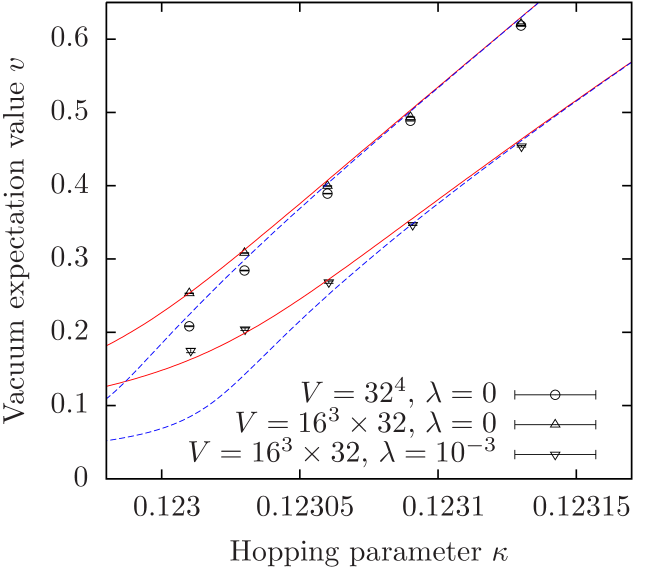
In Fig. 6.7 the one-loop LPT predictions for the vacuum expectation value are plotted versus the hopping parameter for different lattice volumes in the case of a vanishing and a non-vanishing value of the quartic coupling constant . These perturbative results are compared to corresponding results obtained in direct Monte-Carlo simulations and good agreement is observed.
From these findings one can conclude that the here presented approach of calculating the vev by means of lattice perturbation theory at one-loop order already provides a reasonably good description of the behaviour of the model in the broken phase within the weakly interacting regime.
6.2.2 Higgs boson self-energy from one-loop LPT
In this section the Higgs propagator, and thus the Higgs boson self energy , will be computed to one-loop order in lattice perturbation theory. For that purpose one usually decomposes the full Higgs propagator into an infinite sum of products of bare propagators and one-particle-irreducible diagrams666Again, vacuum bubbles are canceled with the denominator in Eq. (6.25) up to neglected finite volume terms., as illustrated in Fig. 6.8. A one-particle-irreducible diagram, usually denoted as 1PI-diagram, is an amputated, connected diagram that cannot be disconnected by neglecting a single internal line only, where the property ’amputated’ means that the external propagators have been divided out. In the given illustration, however, the notion 1PI has, more precisely, to be understood as the sum of all one-particle-irreducible diagrams with exactly two legs (prior two their amputation), being Higgs-legs carrying the momentum . For clarification it is remarked that the expansion point around which the total action is split up into the Gaussian and the interacting contribution is assumed here to be the true vacuum expectation value .

By virtue of this decomposition the full Higgs propagator can then be written as an infinite geometric series according to
| (6.37) |
where the so-called self-energy is the sum of the aforementioned one-particle-irreducible diagrams. Summing this series is then straightforward yielding the result
| (6.38) | |||||
For the calculation of the self-energy one thus needs to identify all one-particle-irreducible diagrams contributing to the Higgs propagator according to the aforementioned decomposition at a given loop order. For the one-loop order these diagrams are depicted in Fig. 6.9.

It is remarked here that the loop order does not coincide with the order in the quartic coupling constant as one sees in Fig. 6.9. While the Higgs- and Goldstone-loop diagrams in the upper row give a contribution proportional to , the Higgs- and Goldstone-loop diagrams in the second row are only proportional to . Here, the analytical expressions of all presented diagrams in Fig. 6.9 will be given, even though the latter two diagrams do not add to the achieved order. This is because other diagrams of order , consisting of more than one loop, have been neglected.
Using the results given in section 6.2 the considered diagrams can be translated into an explicit analytical expression for the self-energy according to
| (6.39) | |||||
| (6.40) | |||||
| (6.41) | |||||
where denotes the squared lattice momentum of the relative momentum and the value of the vacuum expectation value is perturbatively fixed here as described in the preceding section. It is remarked that the given result already contains all contributions up to the orders , , and . The aforementioned Higgs- and Goldstone-loop contributions of order are here given separately in form of the expression which, however, does not have a higher convergence order than , as discussed above.
Examples for the perturbative result of the self-energy are presented in Fig. 6.10. These analytical findings are compared to the corresponding numerical results obtained in direct Monte-Carlo calculations. The latter numerical results on the self-energy have been computed by means of Eq. (6.38), where the underlying propagator has directly been taken from the lattice calculation. In the presented examples two cases, namely a vanishing and a non-vanishing quartic self-coupling constant , are considered. In both cases very good agreement is observed between the numerical and analytical results.
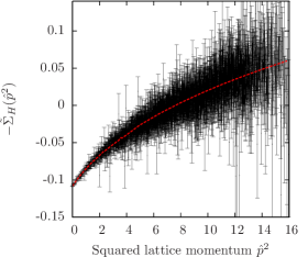 |
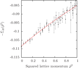 |
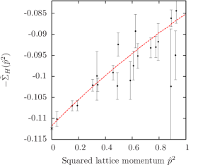 |
| (a) | (b) | (c) |
6.2.3 Quark masses from one-loop LPT
The eventual aim of the evaluation of the considered Higgs-Yukawa model is to determine the range of Higgs boson masses which are consistent with phenomenology. As a consequence the Yukawa coupling constants need to be fine-tuned in order to reproduce the physical top and bottom quark masses. In a first step one can use the tree-level relation given in Eq. (3.84) to choose the bare Yukawa coupling parameters underlying the actual Monte-Carlo calculations as a first guess. To improve this tuning process of the Yukawa coupling constants, however, it would be very useful to have an analytical, next-to-leading order calculation of the quark masses at hand. Here, the analytical result for the top and bottom quark masses from one-loop lattice perturbation theory will be presented.
The first step is thus to calculate the fermion propagator . Following the same standard arguments summarized in section 6.2.2, the full propagator can again be written in terms of the bare fermion propagator given in Eq. (6.30) and the fermion self-energy according to
| (6.44) |
where the fermion self-energy is given as the sum of all amputated, one-particle-irreducible diagrams with two external fermion legs (prior to their amputation) carrying momentum . At one-loop order the only contributing diagrams are the fermion-Higgs and the fermion-Goldstone loops as depicted in Fig. 6.11. It is remarked, that no tad-pole diagrams have to be considered, if the expansion point, around which the total action is split up into a Gaussian and an interacting part, has been chosen as the vacuum expectation value , which is assumed here. In that case all tadpole contributions mutually cancel, since otherwise one would have as discussed in section 6.2.1.

Using the results given in Eq. (6.28-6.30) these diagrams directly translate into the analytical result for the fermion self-energy reading
| (6.45) | |||||
where denotes again the squared lattice momentum of the relative momentum .
To extract the physical mass from this propagator, which is defined through the exponential decay of the time-slice correlator according to Eq. (3.81), one would have to calculate this time-slice correlator from the given one-loop result of the fermion propagator. This can be done by numerically performing a Fourier transformation of the propagator at zero spatial momentum along the time-direction according to
| (6.46) |
with . The latter left-handed fermion propagators underlying the above result are directly obtained from Eq. (6.44) by applying appropriate projection operators according to Eq. (3.80) yielding then
| (6.49) |
From this result it is straightforward to compute the effective fermion masses according to Eq. (6.17).
As an example the perturbatively obtained effective masses are compared to corresponding numerical results in Fig. 6.12, which have been obtained in direct Monte-Carlo calculations. Here the value of the vacuum expectation value appearing in Eq. (6.45) and Eq. (6.49) has not been set to its perturbative prediction derived in section 6.2.1, since that result would be to inaccurate for this purpose here. Instead, it has explicitly been set to its non-perturbatively obtained value as observed in the respective lattice calculations. However, even with this setting the resulting perturbative predictions for the effective masses arising from Eq. (6.45) are not particularly good, as can be observed in Fig. 6.12.
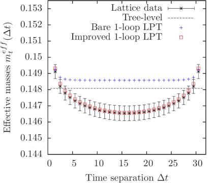 |
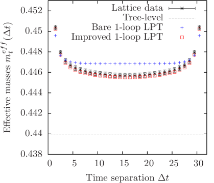 |
| (a) | (b) |
This is the announced example where the considered one-loop calculation in bare perturbation theory does not yield satisfactory results. However, the observed mismatch between the numerical and perturbative one-loop results can significantly be reduced already by an only partial renormalization procedure, where only the bosonic bare masses in Eq. (6.45) will be renormalized. For clarification it is remarked, that a full renormalization procedure is not desirable here, since the actual intention of the presented calculations still is the analytical prediction of the lattice results obtained for a given set of bare model parameters. This can be achieved by replacing the expressions and appearing in the denominators of Eq. (6.45) by the renormalized Higgs boson mass and the renormalized Goldstone mass , which is assumed to be zero for simplicity. The value of the renormalized Higgs boson mass is taken here from the perturbative result of the self-energy derived in the preceding section according777This expression is not exactly equal to the actually introduced definition of the renormalized Higgs boson mass, but coincides with up to small perturbative corrections which, however, do not change the achieved order of the subsequently given result on the self-energy. to . This replacement is perfectly justified in the sense that the achieved convergence order of the original result, which is , is unaltered. Furthermore, the condition has to be imposed in the summation of the Goldstone loop, due to the simplifying assumption which in fact only holds in infinite volume, in order to obtain a finite result of the discrete sum. This modification is justified in the infinite volume limit, since the then arising integral expression can be performed over the aforementioned singularity yielding a finite result due to the sufficiently low order of that singularity. The in this respect improved version of the self-energy then reads
| (6.50) | |||||
The resulting perturbative predictions of the effective masses based on this improved one-loop LPT calculation are also depicted in Fig. 6.12 and one now finds excellent agreement between the numerical and analytical data, allowing thus for a very precise prediction of the fermion masses in the weakly interacting regime of the considered Higgs-Yukawa model.
6.3 Predictions from the effective potential
In section 4.1.1 an expression for the effective potential in the large -limit has been derived, which was used to predict the phase structure in the weakly interacting regime of the considered Higgs-Yukawa model. We will now apply these analytical formulas to predict also the Higgs boson mass at sufficiently small values of the coupling constants and . In particular, we will investigate the dependence of the Higgs boson mass on the model parameters , , and . The knowledge about the latter dependence on the quartic coupling constant will later play a crucial role in the determination of the lowest attainable Higgs boson mass, i.e. the lower Higgs boson mass bound.
6.3.1 Dependence of the Higgs boson mass on and
From perturbation theory it is well known that the Higgs boson mass shift decreases with rising Yukawa coupling constants , according to the qualitative one-loop perturbation theory result given in Eq. (3.83). From this result one can, however, not conclude that the Higgs boson mass itself would also decrease with growing Yukawa coupling constants. In fact, the opposite is the case provided that the cutoff and the quartic self-coupling constant are held constant. This is because the phase transition line is also shifted when the Yukawa coupling parameters are varied, translating directly into an alteration of the bare mass parameter associated to the shifted phase transition point, as will be discussed in the following.
For the purpose of clarification we consider again the effective potential given in Eq. (4.45), which has been calculated in terms of the amplitudes and in the large -limit with degenerate Yukawa coupling constants and . Since we are here only interested in considering the broken phase with and , a less general expression is sufficient for this purpose. For convenience we therefore define , which then simplifies to
| (6.51) |
up to constant terms with the fermionic contribution given as
| (6.52) | |||||
This result follows from Eq. (4.45) when setting to zero. Moreover, the original result has been extended here to the non-degenerate case with .
For a given value of the vacuum expectation value , and thus for a fixed location of the minimum of according to
| (6.53) |
one can then trivially establish the relation
| (6.54) |
between the bare mass parameter , the given vev , and the coupling constants and . It is remarked that the relations in Eq. (6.53-6.54) hold, of course, only up to the considered order of the underlying calculation of the effective potential and moreover only for sufficiently large lattice volumes, where fluctuations around the minimum of can be neglected, which shall, however, be assumed to be the case in the following.
An estimate for the Higgs boson mass can then be obtained from the curvature of the effective potential at its minimum yielding
| (6.55) |
In fact, the curvature of the effective potential gives rather the value of the inverse Higgs propagator at which is, however, directly related to the Higgs boson mass apart from the renormalization factor and the fact that the actual Higgs boson mass is determined at a non-zero momentum configuration as discussed in section 3.4. For our purpose here it is sufficient to neglect these details and to consider as a reasonable estimate for the Higgs boson mass.
From the given finding in Eq. (6.55) one obtains an analytical prediction for the dependence of the Higgs boson mass on the quartic coupling parameter and the Yukawa coupling constants for a given value of the vev . This approach allows to discuss the parameter dependence of the Higgs boson mass for a fixed cutoff , which is directly related to the vev according to Eq. (3.58-3.59) yielding apart from the contribution of the renormalization constant being, however, close to one in the here considered model parameter setups.
In order to test the validity of the analytically predicted dependence of the Higgs boson mass on the degenerate Yukawa coupling constant at a fixed value of the vev , i.e. at an almost fixed value of the cutoff , the aforementioned analytical calculations are compared to corresponding results of direct Monte-Carlo calculations in Fig. 6.13. Both, the analytical as well as the numerical calculations have been performed on a -lattice with , , and degenerate Yukawa coupling constants. The value of the vev has been adjusted here to correspond to an associated cutoff of approximately , which is a typical value for the later determination of the lower Higgs boson mass bounds.
In Fig. 6.13a the numerical and analytical results on the Higgs boson mass shift , defined according to the definition in Eq. (3.83), are shown together with the corresponding bare mass parameters , tuned here to yield the desired value of the vev , versus the squared degenerate Yukawa coupling constant and very good agreement is observed. The same is true for the Higgs boson mass itself, which is presented in Fig. 6.13b.
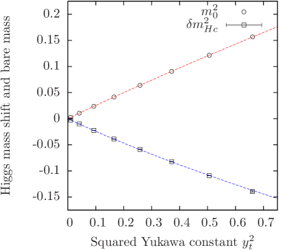 |
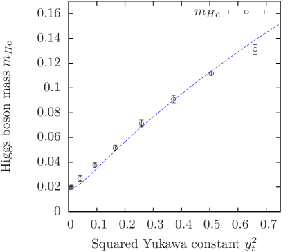 |
| (a) | (b) |
As expected from the qualitative result in Eq. (3.83) the mass shift decreases quadratically with rising Yukawa coupling constants. The Higgs boson mass itself, however, grows with increasing as seen in Fig. 6.13b. As mentioned earlier, the reason is that the effect on the Higgs boson mass induced by the change of the mass shift is overcompensated by the shift of the phase transition line when varying the Yukawa coupling constant while holding and fixed. For constant cutoff and quartic self-coupling constant the resulting shift of the bare mass parameter is presented in Fig. 6.13a.
So far, the presented results have been determined in the mass degenerate case, i.e. for , which is easier to access numerically. This brings up the question of how the results on the Higgs boson mass are influenced when pushing the top-bottom mass split to its physical value, i.e. . From the qualitative result in Eq. (3.83) one expects the Higgs boson mass shift to grow quadratically with decreasing and that is exactly what is observed in Fig. 6.14a. Here, the bare top quark Yukawa coupling constant , the quartic coupling parameter , and the cutoff , more precisely the vev , are held constant, while is lowered to the physical ratio of .
The numerical data for the Higgs boson mass shift are in good agreement with the predictions based on the effective potential in Eq. (6.51), which are depicted by the dashed lines in Fig. 6.14a. Again, the Higgs boson mass itself does not increase but decrease with decreasing as shown in Fig. 6.14b due to the shift of the bare mass parameter as discussed earlier.
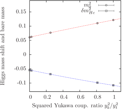 |
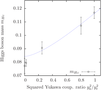 |
| (a) | (b) |
From the very nice correspondence between the numerical and analytical results presented in Fig. 6.13 and Fig. 6.14 one can conclude that the effective potential given in Eq. (6.51) gives a good quantitative description of the considered model even at , at least in the weakly interacting regime of the model at vanishing bare quartic self-coupling constant .
6.3.2 Dependence of the Higgs boson mass on
We now turn to the dependence of the Higgs boson mass on the quartic self-coupling parameter. From the qualitative result in Eq. (3.83) one expects the mass shift to grow linearly to lowest order with increasing values of . This expectation is again explicitly checked by direct Monte-Carlo simulations. In Fig. 6.15a the numerical results on the Higgs boson mass shift and the bare mass are presented versus the quartic coupling parameter . These data were obtained on a -lattice with approximately constant cutoff, i.e. for an approximately constant vev , and degenerate Yukawa coupling constants fixed according to the tree-level relation in Eq. (3.84) aiming at the reproduction of the phenomenological value of the top quark mass. One clearly observes the expected linear increase of the mass shift with rising quartic coupling constant, as expected.
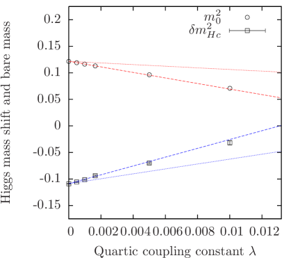 |
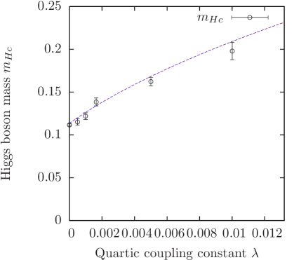 |
| (a) | (b) |
As a first approach the presented numerical data are again compared to the analytical predictions from the effective potential given in Eq. (6.51). The corresponding analytical expectations are depicted by the dotted curves in Fig. 6.15a. Qualitatively, the analytical calculation correctly describes the behaviour of and . On a quantitative level, however, there is a huge discrepancy between the analytical predictions and the corresponding numerical results concerning both, the mass shifts as well as the bare masses.
The origin of this discrepancy is that the approximation of the bosonic contributions to through , which was justified in the limit considered in section 4.1, is just too crude at and . In fact, the given large result for the effective potential does not even contain all contributions of order . Here, the idea is thus to improve the analytical prediction to a practically sufficient level by determining all contributions to the effective potential being of order .
For that purpose we go back to the definition of the effective potential given in Eq. (4.12). Since we consider here only the dependence on the constant mode, the amplitude of which is specified by the parameter , the latter definition simplifies to
| (6.56) | |||||
with and . The corresponding expressions for the Gaussian and the interacting contributions and are then given as
and
| (6.58) | |||||
in the here considered notation.
As already discussed in section 4.1.1 a diagrammatic expansion of this effective potential can then be obtained by expanding into a power series. Here we are only interested in all those diagrams being of order . For the purpose of a brief overview they are sketched in Fig. 6.16. Both depicted diagrams are of first order in , the one on the right, however, does not depend on the parameter in the chosen decomposition of the total action in Eq. (6.56). It will therefore be neglected in the following. Calculating thus only the contributions of the remaining diagram then yields the result
| (6.59) | |||||
| (6.60) | |||||
| (6.61) |
where the relation was used to raise the contributions from the considered diagrams to the exponent and thus into the effective action without changing the achieved order in . The given expression for now contains all contributions of order . For clarification it is pointed out that contributions of the form with are explicitly not meant to be covered by the notation . It is further remarked that the numbers in the nominators of Eq. (6.60-6.61) arise from the underlying combinatorics of the four point vertex.
There is only one subtlety about the expressions in Eq. (6.59-6.61) that should be improved, in order to extend the applicability of the given analytical formulas. The problem is that the considered expansion breaks down as soon as the bare mass becomes negative. The reason is that the Gaussian integration in Eq. (6.56) induced by the contribution becomes divergent in that case. Though this scenario is not encountered in Fig. 6.15 due to the presented bare quartic coupling constants being chosen sufficiently small, it will later play a role in section 6.5, where negative bare mass parameters will be encountered. We therefore shall discuss this issue already at this point.

The aforementioned problem can be fixed by a partial renormalization procedure, where one simply replaces the bare mass in the denominators of Eq. (6.60-6.61) with the renormalized Higgs boson mass and the renormalized Goldstone mass , respectively. More precisely, we assume here a vanishing mass for the case of the Goldstone contribution and take the Higgs boson mass estimate in Eq. (6.55) as the value for the renormalized Higgs boson mass leading then to the improved expression for the effective potential
| (6.62) | |||||
| (6.63) | |||||
| (6.64) |
For clarification it is pointed out that the considered replacements are justified, since they do not change the achieved order of the final result. This is because the bare mass , which is fixed according to Eq. (6.54) for a given value of the vev , coincides with zero and up to corrections of order .
The Higgs boson mass estimate can then be determined in a self-consistent manner by iteratively calculating the effective potential from Eq. (6.62) based on the value for that has been obtained from Eq. (6.55) in the preceding iteration.
The results on the mass shifts and bare masses obtained by the improved effective potential in Eq. (6.62) are shown in Fig. 6.15a depicted by the dashed lines. The improved results are in very good agreement with the numerical data. Of course, this correspondence only holds for sufficiently small values of the quartic self-coupling constant according to the neglection of higher order contributions. It is also interesting to note that the -dependence of the Higgs boson mass itself is already well described by the large potential in Eq. (6.51) as seen in Fig. 6.15b. This is because the contribution to arising from the corrections to and , as induced by the consideration of and , exactly cancels. From the above observations one can thus conclude that the improved effective potential in Eq. (6.62) gives a good quantitative description of the Higgs boson mass in the weakly interacting regime of the considered Higgs-Yukawa model.
The main result of the present section is, that the lightest Higgs boson masses are indeed observed at vanishing bare quartic coupling constant, i.e. . This can be inferred from the analytical result in Eq. (6.62). Moreover, it can directly be observed in Fig. 6.15b, where the dependence of the Higgs boson mass on the bare parameter is explicitly presented. That this dependence remains monotonically rising with also at much larger values of the bare quartic coupling constant will explicitly be demonstrated in section 7.2. Anticipating the latter observation at this point, the search for the lower Higgs boson mass bound can therefore safely be restricted to the scenario of vanishing bare quartic coupling constant, i.e. .
Finally, it is remarked that the decomposition of the total action into a Gaussian and an interacting contribution as given in Eq. (6.56) is not unique as already discussed in section 4.1.1. For instance, terms of the form and could also have been assigned to the Gaussian part , which would then have led to a different result for matching the here provided expression only up to the considered order . It has, however, turned out in practice that the effective potential given in Eq. (6.62) yields better agreement with the here considered direct Monte-Carlo calculations than this alternative approach.
6.4 Lower Higgs boson mass bounds
Given the knowledge about the -dependence of the renormalized Higgs boson mass, which was investigated in the preceding section coming to the concluding result that the lightest Higgs boson masses are indeed obtained at vanishing bare quartic self-coupling constant as expected, we can now safely determine the cutoff-dependence of the lower Higgs boson mass bound by evaluating the Higgs boson mass at for several values of the cutoff .
This will be done for the mass degenerate case with and in section 6.4.1 as well as for the actual physical situation with and in section 6.4.2. However, a couple of restrictions limit the range of accessible energy scales. On the one hand all particle masses have to be small compared to to avoid unacceptably large cutoff effects, on the other hand all masses have to be large compared to the inverse lattice side lengths to bring the finite volume effects to a tolerable level. As a minimal requirement we demand here that all particle masses in lattice units fulfill
| and | (6.65) |
which already is a rather loose condition in comparison to the common situation in QCD, where one usually demands at least .
It will, however, be seen later that even these less restrictive requirements cannot be fulfilled in the actual physical setup , with our available resources in contrast to the mass degenerate case with equal top and bottom quark masses. This is due to the immense lattice size that would be required to accommodate the bottom quark with a mass of and the top quark with a mass of simultaneously on the same lattice.
Besides this technical difficulty there is also the conceptual problem in the non-degenerate case that the complex phase of the fermion determinant is not bound to real values. Though the fluctuation of the complex phase seems to be strongly suppressed in actual Monte-Carlo simulations of physical interest as discussed in section 3.6.2, the true impact of this complex phase on the considered observables remains unclear in the context of the large scale computations that are to be performed here.
We therefore perform the major part of the lower Higgs boson mass bound analysis in the mass degenerate case with and .
6.4.1 Degenerate case with and
As a consequence of the chosen requirements given in Eq. (6.65) concerning the cutoff , the lattice side lengths , and the lightest and heaviest masses in the particle spectrum we will be able to investigate the lower Higgs boson mass bound at energy scales ranging approximately from to . This follows when assuming a lattice with side lengths , a degenerate top/bottom quark mass of , and a Higgs boson mass in the range of to . These numbers are justified aposteriori by the final results of the obtained Higgs boson mass bounds. According to Eq. (3.58-3.59) the aforementioned range of energy scales is directly related to an interval of eligible values of the inverse vev . Assuming888This estimate is provided here only for the purpose of a first orientation. In the actual evaluation of the lattice calculations the respective value of is, of course, explicitly determined. a Goldstone renormalization constant of the allowed values of the vacuum expectation value are given here as .
In the following we will consider a series of Monte-Carlo runs performed at five different values of the hopping parameter to cover the whole specified interval of energy scales. These lattice calculations will be run on various lattice volumes to study the finite size effects and to allow ultimately for an infinite volume extrapolation of the obtained lattice results. The model parameters underlying these Monte-Carlo calculations are listed in Tab. 6.5. In this scenario the degenerate Yukawa coupling constants have been fixed according to the tree-level relation in Eq. (3.84) aiming at the reproduction of the phenomenologically known top quark mass and the quartic coupling constant has been set to for the aforementioned reasons.
| 1/v | ||||||||
|---|---|---|---|---|---|---|---|---|
| 0.12301 | 10,12,14,16,18,20,24,32 | 32 | 1 | 0 | 0.35285 | 1 | ||
| 0.12303 | 10,12,14,16,18,20,24,32 | 32 | 1 | 0 | 0.35288 | 1 | ||
| 0.12306 | 10,12,14,16,18,20,24,32 | 32 | 1 | 0 | 0.35292 | 1 | ||
| 0.12309 | 10,12,14,16,18,20,24,32 | 32 | 1 | 0 | 0.35296 | 1 | ||
| 0.12313 | 10,12,14,16,18,20,24,32 | 32 | 1 | 0 | 0.35302 | 1 |
The numerically obtained Higgs correlator masses resulting in these lattice calculations are presented in Fig. 6.17. To illustrate the influence of the finite lattice volume those results, belonging to the same parameter sets, differing only in the underlying lattice size, are connected by dotted lines to guide the eye. From these findings one learns that the model indeed exhibits strong finite volume effects when approaching the upper limit of the defined interval of reachable cutoffs, as expected, i.e. when the size of the correlation length of the Higgs particle becomes comparable to the lattice side extension.
In Fig. 6.17 the Higgs boson masses have actually been given in units of the measured vacuum expectation value , and the obtained data were plotted versus . This presentation is equivalent to showing the Higgs boson masses in physical units versus the cutoff up to a global scale factor and up to corrections induced by a non-constant renormalization factor . The chosen illustration, however, allows for direct comparability between the given numerical results and the analytical predictions derived from the effective potential in the preceding section which are depicted by the dashed curves in Fig. 6.17. By comparing the analytical and numerical results to each other one observes that the analytical calculations describe the actually measured cutoff dependence of the Higgs boson masses very well. The analytical calculations also correctly predict the observed finite volume effects of the Higgs boson mass . From this finding it can be concluded that the behaviour of the model is very well understood by means of the effective potential calculations discussed in section 6.3.
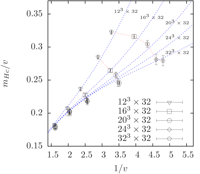
To obtain the desired lower Higgs boson mass bounds these finite volume results on the Higgs boson mass have to be extrapolated to the infinite volume limit and the renormalization factor has to be properly considered. For that purpose the finite volume dependence of the Monte-Carlo results on the renormalized vev and the Higgs boson mass is explicitly shown in Fig. 6.18a and Fig. 6.18b, respectively. One sees in these plots that the finite volume effects are rather mild at corresponding to the lowest presented cutoff in Fig. 6.17 with on the -lattice while the renormalized vev, and thus the associated cutoff , as well as the Higgs boson mass itself vary strongly with increasing lattice size at the smaller presented hopping parameters.
It is well known from lattice investigations of the pure -theory [148, 149, 124] that the vev as well as the mass receive strong contributions from the Goldstone modes, inducing finite volume effects of algebraic form starting at order . The next non-trivial finite volume contribution was shown to be of order . In Fig. 6.18 the obtained data are therefore plotted versus . Moreover, the aforementioned observation justifies to apply the linear fit ansatz
| (6.66) |
to extrapolate these data to the infinite volume limit, where the free fitting parameters and with the subscripts and refer to the renormalized vev and the Higgs boson mass , respectively.
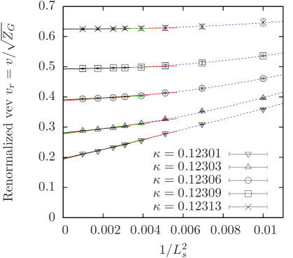 |
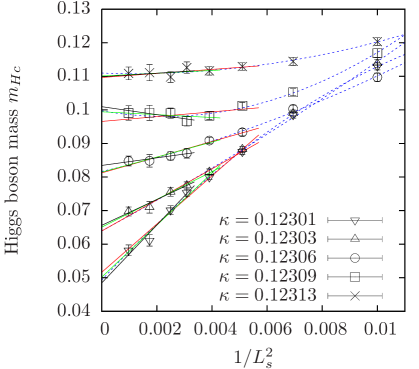 |
| (a) | (b) |
To respect the presence of higher order terms in only the largest lattice sizes are included into this linear fit. Here, we select all lattice volumes with . As a consistency check, testing the dependence of the resulting infinite volume extrapolations on the choice of the fit procedure, the threshold value is varied. The respective results are listed in Tab. 6.6. Moreover, the parabolic fit ansatz
| (6.67) |
is additionally considered. It is applied to the whole range of available lattice sizes. The deviations between the various fitting procedures with respect to the resulting infinite volume extrapolations of the considered observables can then be considered as an additional, systematic uncertainty of the obtained values. The respective fit curves are displayed in Fig. 6.18a,b and the corresponding infinite volume extrapolations of the renormalized vev and the Higgs boson mass, which have here been obtained as the average over the three specified linear fits, are listed in Tab. 6.6.
| Vacuum expectation value | |||||
|---|---|---|---|---|---|
| , | , | , | |||
| Higgs correlator mass | |||||
| , | , | , | |||
However, before the obtained results on the Higgs boson mass can actually be considered as the sought-after lower Higgs boson mass bound , it has to be checked, that the physical top quark mass is actually reproduced in the chosen model parameter setups specified in Tab. 6.5. This is not obvious, since the tree-level relation given in Eq. (3.84) has been used so far to select the value of the bare Yukawa coupling constants underlying the performed lattice calculations.
For that purpose the corresponding finite volume top quark masses999To save numerical resources, only every eighth field configuration has been evaluated in the quark mass analysis. are presented in Fig. 6.19a. Those results belonging to the same parameter sets, differing only in the underlying lattice size, are again connected by dotted lines to guide the eye and the solid horizontal line depicts the tree-level expectation. One clearly observes significant deviations between the latter tree-level expectation and the actual numerical results, in particular on the smaller lattice volumes and for large values of the cutoff.
Here, the presented top quark masses have again been given in units of , while the obtained data were plotted versus , allowing thus for a direct comparison with the analytical predictions derived in section 6.2.3. These analytical expectations are depicted by the dashed lines in Fig. 6.19a and excellent agreement is observed. From this presentation one can deduce that the top quark mass, and thus the renormalized Yukawa coupling constant, decreases slightly with growing cutoff when holding the bare parameters , , and fixed, which is the behaviour that one would have expected in a trivial theory.
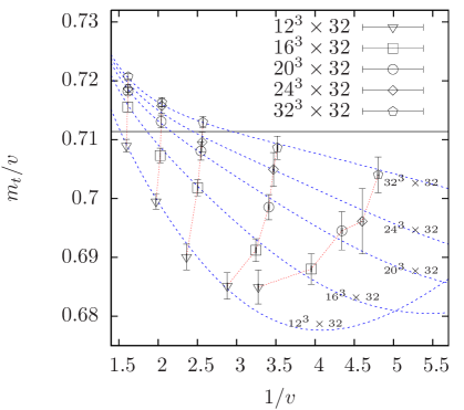 |
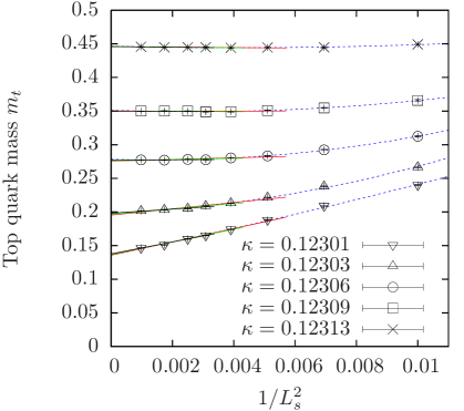 |
| (a) | (b) |
One can in principle exploit the observed very good agreement between the analytical predictions and the actual numerical results on the top quark mass to establish an efficient tuning of the bare Yukawa coupling constants beyond a trial-and-error approach, allowing ultimately to hold the fermion masses constant for each considered cutoff101010Apart from the top quark mass being constrained by the triviality property of the Higgs-Yukawa sector. and lattice volume in some follow-up Monte-Carlo calculations. The aforementioned cutoff dependence of the actually measured top quark mass, however, becomes less prominent as the lattice volume increases and we will shortly see that in the infinite volume extrapolation the targeted value of the top quark mass is actually reproduced within the given errors. For that reason such an improvement has not been investigated in this study.
| Top mass | |||||
|---|---|---|---|---|---|
| , | , | , | |||
The already announced infinite volume extrapolation of the top quark mass is here performed in exactly the same manner as described above. The numerically obtained finite volume top quark masses are plotted versus in Fig. 6.19b together with the parabolic and linear fits arising from the fit approaches in Eq. (6.66) and Eq. (6.67). The corresponding results of the appropriately relabeled fit parameters are listed in Tab. 6.7 and the final infinite volume extrapolations, also shown in that table, are again determined as the average over the three linear fit results as specified by the three listed values of the threshold parameter .
The obtained infinite volume extrapolations of the top quark mass are presented in Fig. 6.20a depicted by the square symbols. From these results one learns that the numerically computed top quark masses, extrapolated to the infinite volume limit, are indeed consistent with the targeted value of the top quark mass within the given errors as already stated above, thus finally justifying the underlying fixation of the bare Yukawa coupling constant according to the tree-level relation in Eq. (3.84), at least for the here achieved accuracy.
The main result of this section, however, is presented in Fig. 6.20b, showing the cutoff dependence of the lower Higgs boson mass bound as obtained from the infinite volume extrapolations summarized in Tab. 6.6. These numerical results, depicted by the square symbols here, are compared to the analytical infinite volume predictions obtained from the effective potential given in Eq. (6.51-6.52), where the discrete sums have been replaced by corresponding integrals to obtain the analytical infinite volume predictions.
According to the relatively good agreement between the presented analytical and numerical findings it is furthermore reasonable to show also some analytical infinite volume predictions for a couple of other physical setups, which will not be backed up by equally precise Monte-Carlo calculations here, with the only exception of the, however far less accurate, data depicted by the circular symbols which will be discussed below. In Fig. 6.20b three additional setups with varying values of and are additionally presented to study the influence of these parameters on the lower Higgs boson mass bound. One can infer from this presentation that the number of fermion generations (or here equivalently the number of colours) as well as the bottom-top mass splitting have a strong impact on the lower mass bound.
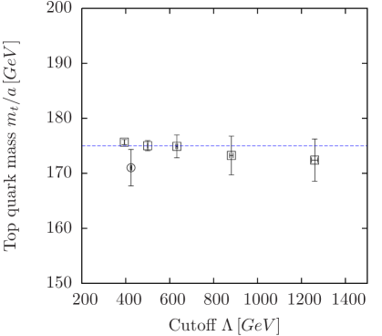 |
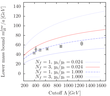 |
| (a) | (b) |
The solid curve in Fig. 6.20b with and comes closest to the actual physical situation in the Standard Model and one observes that the lower Higgs boson mass bound is significantly increased in this physically more relevant scenario as compared to the so far discussed degenerate case with . The aforementioned circular symbols in Fig. 6.20 actually represent some infinite volume extrapolated results of corresponding lattice data computed in this latter physical setup, as will be discussed in the subsequent section. Though this latter numerical result on the lower mass bound, available here only at one selected cutoff parameter , indeed tends to be larger than the previously presented numbers, as expected from the analytical predictions, the associated uncertainty of this result is too large to clearly distinguish between the considered degenerate and non-degenerate scenarios.
The concluding remark of this section is thus that the cutoff dependence of the infinite volume lower Higgs boson mass bounds can indeed be calculated by means of the applied lattice techniques at least in the mass degenerate case for an interval of cutoffs ranging approximately from to . From the obtained results it can be concluded that the lower Higgs boson mass bound is a manifest property of the pure Higgs-Yukawa sector that evolves directly from the Higgs-fermion interaction for a given Yukawa coupling parameter. For growing cutoff this lower mass constraint rises monotonically with flattening slope as expected from perturbation theory. Moreover, the quantitative size of the (analytically obtained) lower bound for and depicted by the solid line in Fig. 6.20 is comparable to the magnitude of the perturbative results based on vacuum stability considerations [71] which were discussed and presented in section 1. A direct quantitative comparison is, however, non-trivial due to the different regularization schemes, blocking a direct matching of the underlying cutoff parameters .
6.4.2 Physical setup with and
In the preceding section the lower Higgs boson mass bound has been derived for the degenerate case with equal top and bottom quark masses and . Now, we want to extend these previous considerations in two respects. First of all, we intend to reproduce the phenomenologically known values for both, the top quark and the bottom quark masses, by setting the ratio of the Yukawa coupling constants to its phenomenological value, which will be done here again with the help of the tree-level relation in Eq. (3.84). The other modification is that we will now properly respect the so far neglected colour index of the fermions by setting the fermion generation number to three, i.e. , in the subsequent lattice calculations. For clarification it is pointed out, that there are still no gauge fields included within the model. It is only the multiplicity induced by the fermion colour index that will now appropriately be accounted for.
However, corresponding lattice calculations in this physical setup are much more demanding than the computations performed in the mass degenerate case. From a technical perspective this is mainly due to the much larger condition numbers in the non-degenerate scenario as observed in section 5.2.2. Moreover, there is the conceptual uncertainty arising from the fluctuating complex phase of the fermion determinant as pointed out in section 3.6.2. Finally, the huge discrepancy between the top and bottom masses would require enormous lattice volumes to accommodate both particles simultaneously on the same lattice, at least when retaining the minimal conditions in Eq. (6.65).
| 0.122204 | 10 | 32 | 3 | 10620 | 0 | 0.35169 | 0.024 |
| 0.122204 | 12 | 32 | 3 | 10860 | 0 | 0.35169 | 0.024 |
| 0.122204 | 14 | 32 | 3 | 6680 | 0 | 0.35169 | 0.024 |
| 0.122204 | 16 | 32 | 3 | 4600 | 0 | 0.35169 | 0.024 |
| 0.122204 | 18 | 32 | 3 | 2200 | 0 | 0.35169 | 0.024 |
| 0.122204 | 20 | 32 | 3 | 1240 | 0 | 0.35169 | 0.024 |
Subsequently, it will nevertheless be tried to determine a lower Higgs boson mass bound also in this physically more significant setup. For that purpose a series of lattice calculations has been performed on different lattice volumes to allow later for an infinite volume extrapolation. The model parameters underlying these computations are listed in Tab. 6.8. Here, only one value for the hopping parameter , and thus for the associated cutoff , has been investigated due to the aforementioned difficulties. The given model parameters were chosen such that the resulting cutoff becomes approximately , since this setting clearly obeys the requirement in Eq. (6.65), while generating the least prominent finite volume effects of all parameter setups considered in the preceding section.
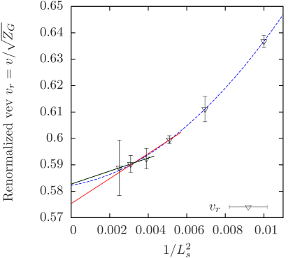 |
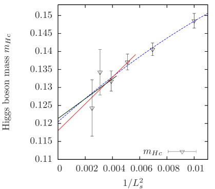 |
| (a) | (b) |
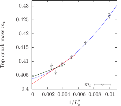 |
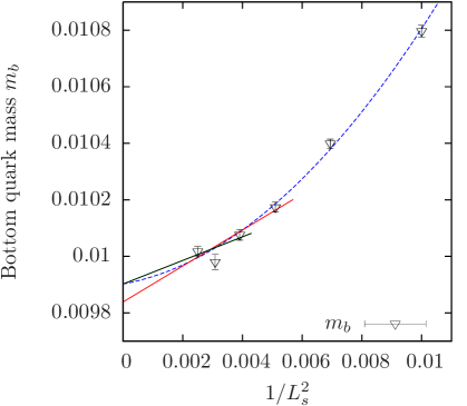 |
| (c) | (d) |
The corresponding numerical results of the lattice calculations specified in Tab. 6.8 are presented in Fig. 6.21, where the renormalized vev , the Higgs correlator mass , as well as the top and bottom quark masses are plotted versus . One directly observes that the obtained results are distinctly less accurate than the corresponding results in the mass degenerate case, which is due to the much lower statistics obtained in this scenario. At the same time the finite volume effects are clearly stronger, as expected, thus rendering the infinite volume extrapolation of the given numerical results more problematic.
For the latter purpose we apply again the linear and parabolic fit approaches given in Eq. (6.66) and Eq. (6.67). The fit curves resulting for the respective observables are also depicted in Fig. 6.21 and the corresponding results of the extrapolation to the infinite volume limit are listed in Tab. 6.9. In principle, it is tried here to apply the same extrapolation strategy already discussed in the preceding section. Due to the smaller number of available lattice results, however, the linear fit procedure has been performed with only two values of the threshold parameter as presented in the aforementioned table. The final extrapolation results have then been obtained by averaging over the one parabolic and the two linear fits. The translation of these numbers into physical units is also provided in Tab. 6.9.
| observable | , | , | Final result of ext. | |
| Final results of extrapolation in physical units | ||||
As intended, the phenomenological values of the top and bottom quark masses are approximately reproduced, at least clearly for the bottom quark mass, while the top quark mass may require some more tuning of the underlying bare Yukawa coupling constant. One can also observe that the obtained lower Higgs boson mass bound tends to be somewhat larger than the corresponding result in the mass degenerate case. This has been anticipated by the analytical predictions depicted in Fig. 6.20, where the here obtained final results have already been presented in comparison with the lower mass bounds arising in the degenerate case. The associated uncertainty of the presented result, however, is too large to clearly distinguish between the analytical curves with and illustrated in Fig. 6.20.
6.5 Model extension by higher order bosonic self-interaction terms
So far, the given results on the lower Higgs boson mass bound have been derived in the Higgs-Yukawa model as originally specified in section 3.3. In particular, the self-interaction of the scalar field is completely determined by the -coupling term. Since the Higgs-Yukawa sector can, however, only be considered as an effective field theory with a non-removable cutoff due to its triviality property as discussed in section 1, the usual renormalization arguments do not exclude the consideration of higher dimensional operators in the framework of this effective theory. This observation then opens up the question of how the obtained lower Higgs boson mass bounds would be altered when extending the underlying model by incorporating such higher dimensional operators into the theory.
To give at least a partial answer in this matter we will study here the effect of the additional and coupling terms. They are included into the original form of the purely bosonic part of the lattice action given in Eq. (2.49) yielding then the extended lattice action
Here, we will begin with deriving some analytical predictions of the effect of these new coupling terms. For that purpose the effective potential calculation performed in section 6.3.2 is revisited. The idea is to calculate all contributions to as defined in Eq. (6.56), that are of order , , or . For that purpose the total action is again split up into a purely Gaussian contribution as already given in Eq. (6.3.2), the extended tree-level part , and the remaining interacting contribution , where the latter now becomes
The next step is then the identification of all diagrams arising from the expansion of and contributing to at the considered orders. For the case of the -coupling term these diagrams are sketched in Fig. 6.22, while the corresponding diagrams generated by the four point vertex have already been illustrated in Fig. 6.16. The -diagrams are not explicitly listed here, since they are fully analogous to the already presented ones. It is further remarked that the contribution on the very left in Fig. 6.22 does actually not generate any dependence on and could thus also be neglected for our purpose here. It is nevertheless computed just for the sake of uniformity.

Following the same steps already discussed in section 6.3.2 one then directly arrives at the final result
for the effective potential including all contributions up to the orders , , and , where the Higgs and Goldstone propagator sums and are given as
| and | (6.71) |
Here, the bare mass that one would originally have obtained in the denominators of Eq. (6.71) has again been replaced by the estimates of the renormalized Higgs and Goldstone masses for the same reasons already discussed in section 6.3.2. The so far unspecified coefficients , , and are then given by the multiplicities of the associated diagrams, which have been determined here with the help of some trivial, self-written computer program counting the respective numbers of Wick contractions. The resulting coefficients are listed in Tab. 6.10, where one also finds the numbers and that recover the expression for the effective potential previously presented in Eq. (6.62) for the case of vanishing model extension parameters, i.e. .
| 6 | 6 | – | |||
| 3 | 6 | 15 | |||
| 15 | 9 | – | – | ||
| 45 | 54 | 45 | – | ||
| 15 | 27 | 45 | 105 | ||
| 28 | 12 | – | – | – | |
| 210 | 180 | 90 | – | – | |
| 420 | 540 | 540 | 420 | – | |
| 105 | 180 | 270 | 420 | 945 | |
To check the validity of the given analytical formula in Eq. (6.5) the arising predictions for the Higgs boson mass dependence on the new model parameters and are explicitly compared to corresponding results obtained in direct Monte-Carlo calculations as presented in Fig. 6.23. Here, the parameters and have been varied, while the quartic coupling constant and the targeted quark masses have been kept constant and the hopping parameter has been tuned with the intention to sustain a fixed value of the cutoff . One clearly observes a very good agreement between the numerical and the analytical data at least for sufficiently small values of the respective coupling constants. For the -coupling term the onset of the expected deviation between the numerical and analytical results at larger values of the coupling parameter can also be observed. From these findings one can conclude that the behaviour of the extended model is well understood for not too large values of the coupling parameters.
The derived analytical result for the effective potential given in Eq. (6.5) can now be used to identify those bare model parameters that would generate a given target value of the vev and a given target value of the Higgs boson mass by solving the set of equations
| (6.72) | |||||
| (6.73) |
with respect to the bare model parameters. The solution to these equations is underdetermined. We can therefore assign specific values to some of the parameters. Here, we use this freedom to choose the degenerate Yukawa coupling constants still according to the tree-level relation in Eq. (3.84) aiming at the reproduction of the phenomenological value of the top quark mass and the eight-point coupling parameter is explicitly chosen to zero, i.e. . Furthermore, the constant can freely be chosen from a so far unspecified interval of eligible values.
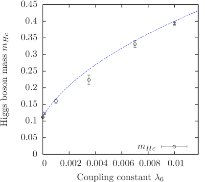 |
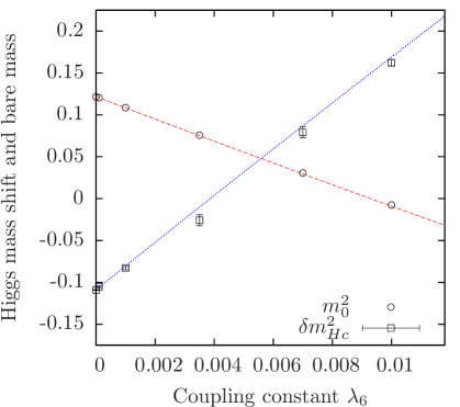 |
| (a) | (b) |
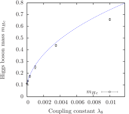 |
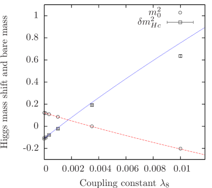 |
| (c) | (d) |
Here, the idea is to find out whether the lower Higgs boson mass bound established in the preceding section can be undercut in the framework of the considered model extension. For that purpose a couple of parameter setups are presented in Tab. 6.11 solving Eq. (6.72-6.73) for different choices of and varying targeted Higgs boson masses , while the choice of the targeted vev is intended to generate a constant cutoff value of approximately . Here, the star symbol in the superscript indicates that the renormalization factor was assumed to be one for the conversion between the vev and the cutoff. In the actual lattice computation the renormalization constant is, of course, fully respected.
| 0.71138 | 1 | 0.14262 | 0 | |||||
|---|---|---|---|---|---|---|---|---|
| 0.71138 | 1 | 0.13188 | 0 | |||||
| 0.71138 | 1 | 0.14912 | 0 | |||||
| 0.71138 | 1 | 0.13836 | 0 | |||||
| 0.71138 | 1 | 0.15345 | 0 | |||||
| 0.71138 | 1 | 0.14268 | 0 | |||||
| 0.71138 | 1 | 0.15561 | 0 |
The proposed model parameter setups in Tab. 6.11 have then been used to configure corresponding direct lattice calculations. The actually obtained numerical results on the cutoff and the Higgs boson mass are finally presented in Fig. 6.24 versus the respective targeted values of the Higgs boson mass. One clearly observes that the lower Higgs boson mass bound can indeed significantly be shifted towards smaller values when extending the model by the considered higher order self-interaction terms. In the presented examples the obtained Higgs boson masses are up to approximately two times smaller than the previously derived lower mass bound discussed in section 6.4.1. This situation occurs here at negative values of the quartic coupling constant . For clarification it is pointed out that a negative value of does not render the model unstable in the here considered cases, since the higher order coefficient was chosen to be positive.
One also learns from the given results that the trial of adjusting arbitrarily small Higgs boson masses by means of the here presented method has failed. This may be due to the existence of a lower Higgs boson mass bound also in the framework of the extended model. It may, however, simply be the analytical determination procedure of the underlying bare model parameters that needs to be further improved. Since the intended retention of the cutoff value has also failed, the latter explanation seems more likely. A direct investigation of this question based on a trial-and-error approach is, however, not very practical, since the generation of the observed low Higgs boson masses requires a precise tuning of the underlying bare model parameters. The latter question thus remains open here.
As a concluding remark it is summarized that the established lower Higgs boson mass bound in the preceding section can clearly be undercut in the here considered model extension. The latter mass bounds can thus not be considered to be universal, in the sense that they are not independent of the specific form of the underlying interactions.
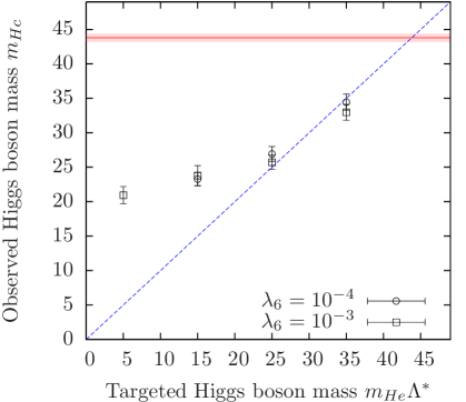 |
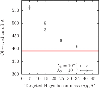 |
| (a) | (b) |
Chapter 7 Results on the upper Higgs boson mass bound
The sought-after upper Higgs boson mass bound and in particular its dependence on the cutoff parameter shall finally be investigated in this chapter. The aforementioned bound will be established here by means of direct lattice calculations performed in the strongly interacting regime of the considered Higgs-Yukawa model as outlined in section 3.4. Before we actually begin with the discussion of the obtained lattice data, it is, however, worthwhile to briefly recall some of the major results concerning the upper Higgs boson mass bound that have already been established in previous lattice investigations.
For the pure -theory, thus neglecting the coupling to the fermions, the latter mass bound has been studied in great detail. Numerous lattice studies, see e.g. Refs. [45, 47, 193] and the references therein, examined in particular the case of an infinite bare quartic self-coupling constant , where the Higgs boson mass is expected to be maximal. By virtue of the cluster algorithm [194, 195] the achieved numerical performance of these investigations could later be enhanced, which finally led to very precise results on the vacuum expectation value and the Higgs boson mass itself [196, 197]. For the orientation of the reader a single number shall be cited here taken from a rather early study [46], which estimated the upper mass bound to be approximately at a cutoff of in the here considered notation.
Accompanied by these numerical investigations the pure lattice -theory has been solved analytically [198, 199, 44] in the sense that most low energy observables can be calculated analytically for any set of bare model parameters, especially for arbitrary values of the bare quartic coupling constant , except for model parameters in the broken phase far away from the critical line. These latter points in the parameter space are, however, not of physical interest with respect to the here considered lattice approach, since the cutoff scale associated to these parameter sets would be low and in particular not large compared to the observable particle masses.
The aforementioned analytical results have been obtained by combining a high temperature expansion with perturbative calculations performed in the framework of renormalized perturbation theory. The latter high temperature calculation expands all quantities in terms of the hopping parameter instead of the quartic coupling constant by cutting off the infinite sum in the expression
| (7.1) |
after a finite number of summands, where denotes the partition function of the pure -theory here. The high temperature expansion can thus be applied to any choice of the bare quartic self-coupling constant , in particular to . Its convergence properties are best for small values of the hopping parameter , i.e. in the symmetric phase. In fact, the respective expansion coefficients for the renormalized mass, the field renormalization factor, and the renormalized quartic coupling constant have explicitly been worked out up to 14-th order [200] and excellent results have been obtained for , where is the critical hopping parameter of the pure -theory for the respective value of . For even larger hopping parameters, however, this approach finally breaks down.
The main finding of this high temperature expansion is that the renormalized quartic coupling constant is always in the perturbative regime at independent of the choice of the bare coupling parameter . The results determined from the high temperature expansion at this value of the hopping parameter can therefore be evolved to larger values of , and thus into the here physically relevant broken phase, by integrating the Callan-Symanzik equations, where the coefficients of the associated -functions can be obtained from renormalized perturbation theory as long as remains within the perturbative regime.
By performing the latter integration of the Callan-Symanzik equations it could be shown that the renormalized quartic coupling constant monotonically decreases with growing hopping parameter , i.e. in the symmetric phase, until it finally vanishes completely at the critical line in full agreement with the triviality picture of the pure -theory. The model thus remains in the perturbative regime for all hopping parameters in the interval . For , i.e. in the broken phase, the renormalized quartic coupling constant increases with growing hopping parameter and the perturbative regime is eventually left at some value .
With this combined approach of high temperature expansion and renormalized perturbation theory it is therefore possible to calculate the Higgs boson mass and the renormalized quartic coupling constant for all values of the bare coupling constant and for all hoping parameters . These calculations have been performed in great detail in Refs. [198, 199, 44] where one can also find extensive listings of the obtained analytical results on the Higgs boson mass111The underlying definitions of the Higgs boson mass and the renormalized quartic coupling constant considered in LABEL:Luscher:1988uq are the quantities and given in Eq. (3.68) and Eq. (3.70). and the renormalized quartic coupling constant at various values of and . Moreover, the logarithmically corrected scaling laws of , , and the vev have also been derived by considering the aforementioned Callan-Symanzik equations in the vicinity of the critical line [198, 199, 44]. For the broken phase with the underlying model being the four-component -theory in infinite volume they read
| (7.2) | |||||
| (7.3) | |||||
| (7.4) |
Combining these scaling laws with the additional finding [44] , where the constant is also provided in LABEL:Luscher:1988uq, one immediately arrives at the analytically expected functional form of the dependence of the Higgs boson mass and the renormalized quartic coupling constant on the cutoff. In the limit and for fixed bare quartic coupling constant it is given as
| (7.5) | |||||
| (7.6) |
where double-logarithmic terms have been neglected, denotes some unspecified scale, and , are constants.
So far, all summarized results refer to the pure -theory. It is thus worthwhile to ask whether these scaling laws still hold in the considered Higgs-Yukawa model including the coupling to the fermions. In that respect it is remarked that the same functional dependence has also been observed in an analytical study [106] of a Higgs-Yukawa model in continuous Euclidean space-time based, however, on an one-component Higgs field. In that study the running of the renormalized coupling constants with varying cutoff has been investigated by means of renormalized perturbation theory in the large -limit. Furthermore, the scaling behaviour of the renormalized Yukawa coupling constant has also been derived. It was found to be
| (7.7) |
where and are again so far unspecified constants and stands here for the renormalized top and bottom Yukawa coupling constants and , respectively, as defined in Eq. (3.82).
In the following sections these analytically derived scaling laws will explicitly be compared to the results of direct lattice calculations performed in the considered Higgs-Yukawa model. In particular, the question of how much the here respected fermion dynamics influences the previously observed results in the pure -theory will be addressed. For that purpose we begin with the details of the Higgs boson mass determination in section 7.1, which are different from the earlier discussed approach applied to the weakly interacting regime of the model. The crucial question, at what values of the bare coupling parameter one actually observes the largest Higgs boson masses, is then considered in section 7.2. Given this knowledge about the -dependence of the Higgs boson mass, the sought-after upper mass bound is then finally established in section 7.3.
7.1 Details of the particle mass determination
In analogy to the discussion in section 6.1 the details of the particle mass determination shall now be discussed for the case of the strongly interacting regime of the considered Higgs-Yukawa sector, with the latter notion referring here to the setting . It is basically tried to follow the same approaches already introduced for the weakly coupling scenario. However, some minor modifications in the aforementioned computation schemes have been conducted to make them successfully applicable also in the here considered case of large quartic coupling constants.
In particular, the Higgs boson mass determination will eventually be based on the analysis of the Higgs propagator as proposed in section 3.4. The reasoning is twofold. Firstly, the latter method yields significantly more stable results on the Higgs boson mass than the alternative extraction scheme based on the Higgs time-slice correlator. Apart from this rather technical downside there is the additional argument that the time-slice correlator is expected to receive significant contributions from lighter states due to the Higgs boson becoming increasingly unstable with an eventually no longer negligible decay width when entering the strongly interacting regime as discussed in section 3.4, thus complicating the approach of determining the Higgs boson mass from the latter time-slice correlator also from a conceptual point of view.
Again, the considered computation schemes will be tested in the framework of direct Monte-Carlo calculations, the model parameters of which are listed in Tab. 7.1. These Monte-Carlo runs have been selected to cover the full range of cutoffs that will be investigated for the actual determination of the upper Higgs boson mass bound in the considered Higgs-Yukawa model.
7.1.1 Analysis of the Goldstone propagator
With respect to the determination of the renormalization constant and the Goldstone mass we follow exactly the same approach introduced in section 6.1.2. As an example the Goldstone propagators obtained in the lattice calculations specified in Tab. 7.1 are presented in Fig. 7.1. These numerical data are again fitted222Again, it is actually the inverse propagator that is fitted with . with the fit formula given in Eq. (6.9), which is based on an heuristically motivated modification of the renormalized one-loop result on the Goldstone propagator of the pure -theory in continuous Euclidean space-time, as detailed in section 6.1.2. One can then already observe from the graphical presentation in Fig. 7.1 that the considered fit ansatz describes the numerical data significantly better than the simple linear fit formula given in Eq. (6.10).
Furthermore, it has already been discussed in the aforementioned section that the propagators should only be considered at small momenta to avoid unacceptably large discretization effects. For that purpose the constant has been introduced, such that the applied fit procedures are restricted to the momenta with . In principle, the constant should be chosen as small as possible. For too small values of , however, the fit procedure becomes unstable. To find an optimal setting for the latter threshold value, the dependence of the fit results on the parameter is listed in Tab. 7.2, where the presented Goldstone mass and the respective renormalization factor have been obtained according to Eq. (3.66) and Eq. (3.67) from the analytical continuation of the lattice Goldstone propagator given by and , respectively.
At first glance one notices that the linear ansatz yields more stable results than . These results are, however, inconsistent with themselves when varying the parameter . One can also observe in Tab. 7.2 that the associated average squared residual per degree of freedom significantly differs from one at the selected values of , making apparent that the simple linear fit ansatz is not suited for the reliable determination of the Goldstone propagator properties.
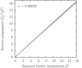 |
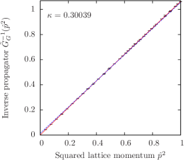 |
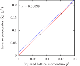 |
| (a) | (b) | (c) |
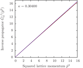 |
 |
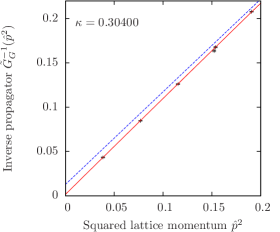 |
| (d) | (e) | (f) |
| fit ansatz | linear fit ansatz | ||||||
|---|---|---|---|---|---|---|---|
| 0.9380(107) | 0.027(15) | 1.00 | 0.9422(5) | 0.067(2) | 2.61 | ||
| 0.9431(52) | 0.028(11) | 0.81 | 0.9507(3) | 0.089(2) | 4.79 | ||
| 0.9457(27) | 0.033(8) | 0.94 | 0.9585(2) | 0.114(2) | 6.19 | ||
| 0.9400(90) | 0.029(10) | 1.41 | 0.9403(4) | 0.066(1) | 4.40 | ||
| 0.9426(36) | 0.032(7) | 1.07 | 0.9476(2) | 0.084(1) | 6.53 | ||
| 0.9478(18) | 0.038(4) | 1.06 | 0.9559(1) | 0.111(1) | 9.67 | ||
In contrast to that the more elaborate fit ansatz yields much better values of being close to the expected value of one as can be seen in Tab. 7.2. Moreover, the results on the renormalization constant and the Goldstone mass obtained from this ansatz remain consistent with respect to the specified errors when varying the constant . For the rest of this chapter the aforementioned quantities and will therefore always be determined by means of the here presented method based on the fit ansatz with a threshold value of , since this setting yields the most stable results, while still being consistent with the findings obtained at smaller values of .
7.1.2 Analysis of the Higgs propagator
Concerning the analysis of the Higgs propagator we will again maintain the same strategy that was already introduced in section 6.1.3. As an example the lattice Higgs propagators as obtained in the Monte-Carlo runs specified in Tab. 7.1 are presented in Fig. 7.2. These numerical data are again fitted333Again, it is actually the inverse propagator that is fitted with . with the fit ansatz given in Eq. (6.11). The only modification that has been conducted is that the Goldstone boson mass parameter appearing in the aforementioned fit formula is not treated as a free parameter here in contrast to the approach originally discussed in section 6.1.3. Instead, it is fixed to the value of resulting from the analysis of the Goldstone propagator by the method described in the previous section. The purpose of this modification is to achieve a higher stability of the considered fit procedure, which otherwise would yield only unsatisfactory results with respect to the associated statistical uncertainties, in contrast to the situation of the weakly interacting regime discussed in section 6.1.3.
Again, one can observe, however less clearly as compared to the previously discussed examples for the case of the Goldstone propagator, that the more elaborate fit ansatz describes the lattice data more accurately than the simple linear fit approach given in Eq. (6.14). This is better observable in the lower row of Fig. 7.2 than in the upper row, where the differences tend to be rather negligible. The reason why the observed differences between the two fit approaches are less pronounced here, as compared to the situation in the preceding section, simply is, that the threshold value was chosen here to be which will be motivated below. This setting is much smaller than the value underlying the previously discussed examples for the Goldstone propagators and causes the linear fit to come closer to the more elaborate ansatz .
The Higgs propagator mass defined in Eq. (3.68) and the Higgs pole mass together with its associated decay width given by the pole of the propagator on the second Riemann sheet according to Eq. (3.66) can then again be obtained by defining the analytical continuation of the lattice propagator as and , respectively. The results arising from the considered fit procedures are listed in Tab. 7.3 for several values of the threshold value . Since the linear function can not exhibit a branch cut structure, however, the pole mass equals the propagator mass and the decay width is identical to zero when applying the linear fit approach. That is the reason why only the Higgs boson mass is presented in the latter scenario.
One observes in Tab. 7.3 that the Higgs boson masses obtained from the linear fit ansatz are again inconsistent with the respective values obtained at varying values of the threshold parameter , thus rendering this latter approach unsuitable for the description of the Higgs propagator. This becomes also manifest through the presented values of the average squared residual per degree of freedom associated to the linear ansatz, which are clearly off the expected value of one, apart from one presented exception444In the first line of Tab. 7.3 one finds for being smaller than the corresponding value for . This is possible although the set of functions parametrizable by is a subset of the corresponding set associated to , since the number of degrees of freedom differs for the latter two fit approaches according to , where is the number of data points and is the number of free fit parameters. at .
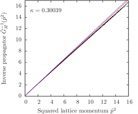 |
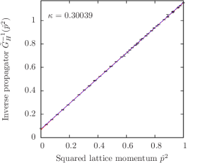 |
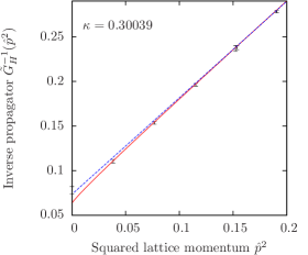 |
| (a) | (b) | (c) |
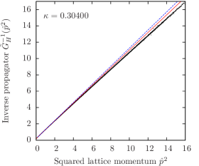 |
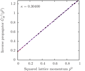 |
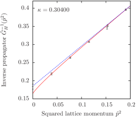 |
| (d) | (e) | (f) |
| Fit ansatz | Fit ansatz | |||||||
|---|---|---|---|---|---|---|---|---|
| 0.30039 | 0.5 | 0.249(6) | 0.253(2) | 0.296(83) | 0.000(0) | 1.17 | 0.253(2) | 1.13 |
| 0.30039 | 1.0 | 0.249(6) | 0.252(2) | 0.253(2) | 0.035(8) | 1.20 | 0.261(2) | 1.62 |
| 0.30039 | 2.0 | 0.249(6) | 0.246(2) | 0.249(2) | 0.062(4) | 1.09 | 0.273(1) | 2.58 |
| 0.30400 | 0.5 | 0.395(5) | 0.405(3) | 0.406(3) | 0.039(13) | 1.43 | 0.399(2) | 1.75 |
| 0.30400 | 1.0 | 0.395(5) | 0.409(1) | 0.410(1) | 0.054(7) | 1.16 | 0.409(1) | 2.23 |
| 0.30400 | 2.0 | 0.395(5) | 0.409(1) | 0.412(1) | 0.087(4) | 1.27 | 0.423(1) | 4.63 |
Again the situation is very different in case of the more elaborate fit ansatz yielding significantly smaller values of . The presented results on the propagator mass as well as the pole mass are also in much better agreement with the corresponding values obtained at varied threshold parameter . Moreover, the values of and are consistent with each other with respect to the given errors. These numbers are also compared to the correlator mass , taken here from the forthcoming discussion in the subsequent section. In the latter comparison significant deviations are observed in some of the presented examples, which is, however, not too surprising due to the large systematic uncertainties of the correlator mass , as discussed in section 7.1.3. It is also pointed out that the statistical errors of the propagator masses are much smaller than for the correlator mass , which is one of the already mentioned arguments to determine the Higgs boson mass by means of the propagator analysis in the strongly interacting regime.
From the findings presented in Tab. 7.3 one can conclude that selecting the threshold value to be for the analysis of the Higgs propagator is a very reasonable choice, which leads to consistent and satisfactory results. This is the setting that will be used for the subsequent investigation of the upper Higgs boson mass bounds to determine the propagator mass as well as the pole mass . It is further remarked that the here chosen value of is much smaller than the value selected in the preceding section for the analysis of the Goldstone propagator. While this large setting worked well in the latter scenario, it leads to inconsistent results in the here considered case and has therefore been excluded from the given presentation.
For clarification it is pointed out that the applied fit formula , which is based on a perturbative calculation performed in continuous Euclidean space-time, is expected to become inconsistent with the lattice data if is chosen too large due to the effect of discretization errors as discussed in section 6.1.3. However, apart from that the perturbative one-loop calculation underlying the fit ansatz is not expected to describe the Higgs propagator very well in the here considered strongly interacting regime of the model, since the one-loop calculation does not even contain all bosonic (momentum-dependent) next-to-leading order contributions, which are the order contributions in this case555The contributions are momentum-independent as discussed in section 6.2.2.. While the main purpose of the Higgs propagator analysis, which is the Higgs boson mass determination, could satisfactorily be achieved with the here presented approach, it would still be worthwhile to extend the analysis at this point by considering a fit ansatz based on a higher order perturbative calculation of the Higgs propagator, since this would further improve the conceptual footing of the applied strategy. In such an extended fit ansatz one should then also include the fermionic contributions.
Finally, the obtained results on the decay width shall be addressed. Unfortunately, one finds in Tab. 7.3 that the extracted decay constants are not consistent when varying the parameter , which would be a minimal requirement to trust in the presented numbers. The problem causing the observed inconsistency is as follows. For a too small threshold value the curvature of the Higgs propagator, which is eventually connected to the decay width through the analytical continuation of the lattice Higgs propagator as discussed in section 3.4, can no longer reliably be resolved due to the statistical uncertainties of the lattice data, leading then ultimately to zero decay width. For larger values of , on the other hand, the effects described in the previous paragraph become the main source for the observed inconsistencies.
One therefore has to conclude that the here presented attempt to determine the decay width of the Higgs boson through the analysis of the lattice Higgs propagator by means of the fit ansatz , which is based on an one-loop perturbative calculation in the pure -theory, was not successful. Two further steps could be performed to improve on this unsatisfactory finding. On the one hand higher statistics would be helpful to reduce the statistical errors of the lattice data. On the other hand, and more importantly, an enhanced fit ansatz based on a higher order perturbative calculation and respecting also the fermionic contributions is required to finally obtain reliable results also in this matter.
This approach for determining , however, will not further be pursued in this study. Instead, Lüscher’s well-known method [109, 110] for determining the decay properties will be applied to the case of the considered Higgs-Yukawa model in chapter 8, where the question of the Higgs boson decay width will finally be revisited.
7.1.3 Analysis of the Higgs time-slice correlator
We now turn to the discussion of the Higgs correlator mass in the strongly interacting regime of the considered Higgs-Yukawa model, referring here to the setting . For that purpose we follow the same steps that have been presented for the scenario of weak interactions in section 6.1.1. At that point it has already been discussed that the time-slice correlation function underlying the definition of the Higgs correlator mass in Eq. (3.74) is actually lacking an obvious connection to the transfer matrix formalism, complicating thus the correct physical interpretation of the considered correlator. For that reason an alternative definition of a Higgs time-slice correlation function manifestly invalidating the aforementioned concern has additionally been investigated as defined in Eq. (6.4). Moreover, two different fit approaches given in Eq. (6.1) and Eq. (6.2) have been applied to extract the correlator mass from the respective correlation function, where the first included also a -independent term in the fit ansatz to account for the contributions of massless states, while the second only contained a single -function. In all considered cases, however, the respective Higgs boson mass was found to be consistent with the other obtained results on that quantity, which allowed for a reliable determination of the Higgs boson mass from the time-slice correlation function in the case of weak interactions.
Here, we want to repeat this previous analysis for the case of the strongly interacting regime of the model. For that purpose the aforementioned time-slice correlation functions and , as observed in the lattice calculations specified in Tab. 7.1, are presented in Fig. 7.3a,d together with the respective fits according to Eq. (6.1) and Eq. (6.2). One observes in these plots that the measured correlation functions are clearly less accurately determined than in the weakly interacting regime discussed in section 6.1.1. One reason explaining this observation is that the Higgs boson mass is much larger here than in the formerly considered scenario, leading thus to a steeper decay of the underlying correlation functions, which renders their reliable determination more demanding with respect to the required number of statistically independent field configurations generated in the lattice calculations.
Moreover, one observes that the fit ansatz in Eq. (6.1), incorporating the constant to respect contributions from massless states, seems to be better suited to describe the actually measured form of the correlation functions. However, the latter constant, as determined in the fit procedure, just turns out to have the wrong sign in the presented examples, implying that one has to be careful with the interpretation of that observation. In fact, the statistical errors of the presented data are just too large to draw a clear conclusion in this matter.
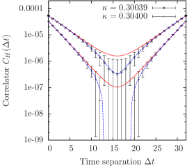 |
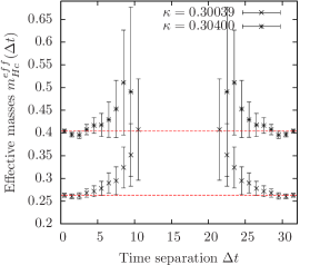 |
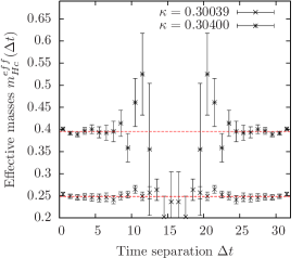 |
| (a) | (b) | (c) |
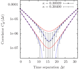 |
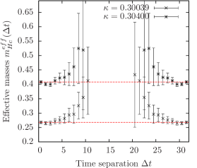 |
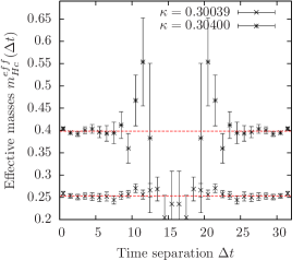 |
| (d) | (e) | (f) |
The associated effective masses as defined in Eq. (6.5) are shown in the other four panels in Fig. 7.3. One sees that the statistical uncertainties associated to the presented effective masses rise quickly with increasing values of , rendering a reliable determination of the correlator mass from these data very problematic. The sought-after correlator masses are therefore again determined here by the overall -fits in Eq. (6.1) and Eq. (6.2) applied to the whole range of time separations . The then resulting values of are compared to the corresponding effective masses in Fig. 7.1 and satisfactory agreement is observed with respect to the specified statistical errors.
The obtained results on the correlator masses are summarized in Tab. 7.4. From this listing one learns that the masses derived from the correlators and with the same fit approach are consistent with each other in the here considered examples. It is, however, remarked that this situation changes dramatically on smaller lattice volumes, where the aforementioned masses differ significantly. An example of the volume dependence of these discrepancies observed in the strongly interacting regime is presented in Fig. 7.4. One sees in the given presentation that these discrepancies vanish in the infinite volume limit, as already discussed in section 6.1.1. The eventual convergence of the considered correlator masses with increasing lattice volume can also be understood from the qualitative argument that the magnetizations defined on neighbouring time-slices should become increasingly correlated when the lattice volume is enlarged. In the infinite volume limit the definitions of and should therefore finally become identical to each other. On too small lattices, however, the two considered correlators yield significantly different results on the Higgs boson mass , thus blocking its reliable determination on the basis of the here presented approach. For clarification it is remarked that the here discussed situation is in contrast to the scenario of the weakly interacting regime, where the aforementioned correlator masses in the investigated lattice calculations, though not explicitly demonstrated in this study, were found to be consistent with each other independently of the considered lattice volume.
| Correlator | from | from | |
|---|---|---|---|
| 0.249(6) | 0.263(4) | ||
| 0.253(6) | 0.268(4) | ||
| 0.395(5) | 0.404(4) | ||
| 0.399(5) | 0.408(4) |
Comparing also the obtained correlator masses arising from analyzing the same correlation functions, however, with the two different fit approaches in Eq. (6.1) and Eq. (6.2) one finds in Tab. 7.4 that the observed deviation is insignificant with respect to the given errors for the case and at most weakly significant in the other case. A similar picture is inferred from Fig. 7.4. As pointed out before one would have expected the resulting correlator mass obtained by including a constant term into the fit ansatz to be larger than in the case, where only a single -function is considered. Since this is not observed here, one has to be careful with the interpretation of the numbers listed in Tab. 7.4. However, the statistical uncertainty of the presented data is just too poor to draw reasonable conclusions in this matter.
Finally, it is concluded that the analysis of the correlation functions and in the here presented manner does not yield a reliable determination of the Higgs boson mass on (small) finite lattice volumes in the here considered strongly interacting regime of the model due to conceptual uncertainties. It also remains unclear how much the obtained correlator masses are systematically influenced by the contributions of lighter states due to the unstable nature of the Higgs boson. Moreover, the considered Higgs correlator masses suffer from much larger statistical uncertainties than the previously discussed propagator masses. In the subsequent investigation of the upper Higgs boson mass bound the Higgs boson mass will therefore always be determined by the method based on the analysis of the Higgs propagator as discussed in section 7.1.2.
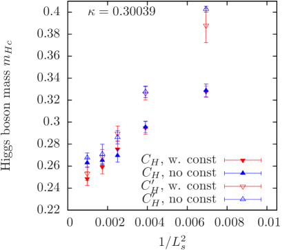 |
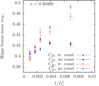 |
| (a) | (b) |
7.2 Dependence of the Higgs boson mass on the bare coupling constant
We now turn to the question whether the largest Higgs boson mass is indeed obtained at infinite bare quartic coupling constant for a given set of quark masses and a given cutoff as one would expect from the results of the effective potential calculation performed in section 6.3.2. Since the underlying formulas of that consideration, however, were derived in the weakly coupling regime, the actual dependence of the Higgs boson mass on the bare quartic coupling constant in the scenario of strong interactions will explicitly be checked here by means of direct Monte-Carlo calculations. The final answer of what bare coupling constant produces the largest Higgs boson mass will then be taken as input for the investigation of the upper mass bound in the subsequent section.
Numerical results on the Higgs propagator mass are therefore plotted versus the bare quartic coupling constant in Fig. 7.5a. The presented data have been obtained for a cutoff that was intended to be kept constant at approximately by an appropriate tuning of the hopping parameter, while the degenerate Yukawa coupling constants were fixed according to the tree-level relation in Eq. (3.84) aiming at the reproduction of the top quark mass. One clearly observes that the Higgs boson mass monotonically rises with increasing values of the bare coupling constant until it finally converges to the result, which is depicted by the horizontal line in the presented plot. From this result one can conclude that the largest Higgs boson mass is indeed obtained at infinite bare quartic coupling constant, as expected. The forthcoming search for the upper mass bound will therefore be restricted to the scenario of .
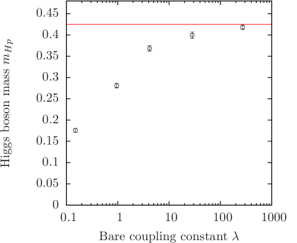 |
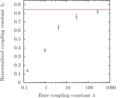 |
| (a) | (b) |
Furthermore, the corresponding behaviour of the renormalized quartic coupling constant as defined in Eq. (3.70) is presented in Fig. 7.5b. As expected one observes a monotonically rising dependence of on the bare coupling constant , eventually converging to the result depicted by the horizontal line. From this finding one can also conclude that the model should remain treatable by means of renormalized perturbation theory also in the regime of large bare quartic coupling constants .
Finally, it is remarked that the numerical computations would have become increasingly difficult with rising values of due to the ever increasing number of required integration steps of the underlying molecular dynamics integration as discussed in section 5.3, if one had tried to integrate the equations of motion in Eq. (5.45-5.46) directly. To circumvent this problem of increasing stiffness of the latter differential equations the alternative approach in Eq. (5.55-5.57) has been used here. With its help different integration step sizes can be assigned to the tangential and radial update steps of the field variables , making the integration possible for any finite value of .
7.3 Upper Higgs boson mass bounds
In this section the cutoff dependent upper Higgs boson mass bound shall finally be determined by means of direct Monte-Carlo calculations performed in the considered Higgs-Yukawa model. Given the knowledge about the dependence of the Higgs boson mass on the bare quartic self-coupling constant , which was studied in the preceding section, the search for the desired upper mass bound can safely be restricted to the scenario of an infinite bare quartic coupling constant, i.e. . Moreover, we will restrict the investigation here to the mass degenerate case with equal top and bottom quark masses and due to the much larger numerical costs of the physically more relevant setup with and , which would clearly exceed those of the corresponding scenario in the weakly coupling regime discussed in section 6.4.2. In the considered setup the Yukawa coupling constants will then again be fixed according to the tree-level relation in Eq. (3.84) aiming at the reproduction the physical top quark mass.
For the same reasons already discussed in section 6.4 the accessible energy scales are again restricted by Eq. (6.65). Employing a top mass of and a Higgs boson mass of below , which will turn out to be justified after the upper mass bound has eventually been established, it should be possible to reach energy scales between and on a -lattice.
| 1/v | ||||||||
| 0.30039 | 12,16,20,24,32 | 32 | 1 | 0.55139 | 1 | |||
| 0.30148 | 12,16,20,24,32 | 32 | 1 | 0.55239 | 1 | |||
| 0.30274 | 12,16,20,24,32 | 32 | 1 | 0.55354 | 1 | |||
| 0.30400 | 12,16,20,24,32 | 32 | 1 | 0.55470 | 1 | |||
| 0.30570 | 12,16,20,24,32 | 32 | 1 | 0 | – | |||
| 0.30680 | 12,16,20,24,32 | 32 | 1 | 0 | – | |||
| 0.30780 | 12,16,20,24,32 | 32 | 1 | 0 | – | |||
| 0.30890 | 12,16,20,24,32 | 32 | 1 | 0 | – | |||
| 0.31040 | 12,16,20,24,32 | 32 | 1 | 0 | – |
For the purpose of investigating the cutoff dependence of the upper mass bound a series of direct Monte-Carlo calculations has been performed with varying hopping parameters associated to cutoffs covering approximately the given range of reachable energy scales. At each value of the Monte-Carlo computation has been rerun on several lattice sizes to examine the respective strength of the finite volume effects, ultimately allowing for the infinite volume extrapolation of the obtained lattice results. In addition, a corresponding series of Monte-Carlo calculations has been performed in the pure -theory, which will finally allow to address the question for the fermionic contributions to the upper Higgs boson mass bound. The model parameters underlying these two series of lattice calculations are presented in Tab. 7.5.
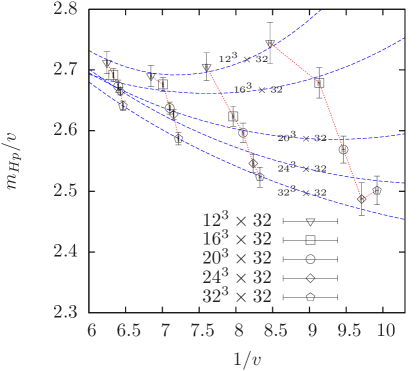 |
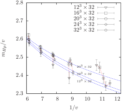 |
| (a) | (b) |
The numerically obtained Higgs boson masses resulting in these lattice calculations are presented in Fig. 7.6, where panel (a) refers to the full Higgs-Yukawa model while panel (b) displays the corresponding results in the pure -theory. To illustrate the influence of the finite lattice volume those results, belonging to the same parameter sets, differing only in the underlying lattice size, are connected by dotted lines to guide the eye. From these findings one learns that the model indeed exhibits strong finite volume effects when approaching the upper limit of the defined interval of reachable cutoffs, as expected.
In Fig. 7.6a one sees that the Higgs boson mass seems to increase with the cutoff on the smaller lattice sizes. This, however, is only a finite volume effect. On the larger lattices the Higgs boson mass decreases with growing as expected from the triviality property of the Higgs sector. In comparison to the results obtained in the pure -theory shown in Fig. 7.6b the aforementioned finite size effects are much stronger and can thus be ascribed to the influence of the coupling to the fermions.
Since the top quark is the lightest physical particle in the here considered scenario it is obvious that the coupling of the Higgs boson to the fermions will generate the major part of the observed finite size effects apart from the Goldstone contributions. The investigation of the setup with the actual physical splitting of the top and bottom quark mass would therefore be even more demanding in the strongly coupling regime than it has been in the previously discussed situation in section 6.4.2, which is one of the reasons why this analysis will not be pursued in the following.
At this point it is worthwhile to ask whether the observed finite volume effects can also be understood by some quantitative consideration. For the weakly interacting regime this could be achieved by computing the effective potential for a given finite volume as discussed in section 6.3. In contrast to that scenario the calculation of the effective potential in terms of the bare model parameters is not directly useful in the present situation, since the underlying perturbative expansion would break down due to the bare quartic coupling constant being infinite here. This problem can be cured by extending the already started partial renormalization procedure in section 6.3.2, such that the bare quartic coupling constant also becomes replaced by its renormalized counterpart. Starting from Eq. (6.62) and assuming a definition of the renormalized quartic coupling constant fulfilling the relation such as the definition given in Eq. (3.70) one can directly derive an estimate for the Higgs boson mass in terms of according to
| (7.8) |
which respects all contributions of order . It is remarked that the contributions and in Eq. (6.62) do not contribute to , as discussed in section 6.3.2. Combining the above result with the expected scaling laws given in Eq. (7.2-7.4) a crude estimate for the observed behaviour of the Higgs boson mass presented in Fig. 7.6 can be established according to
| (7.9) |
where double-logarithmic terms have been neglected and , are so far unspecified parameters.
Since the value of the renormalized quartic coupling constant is not known apriori, the idea is here to use the result in Eq. (7.9) as a fit ansatz with the free fit parameters and to fit the observed finite volume behaviour of the Higgs boson mass presented in Fig. 7.6. These lattice data have been given in units of the vacuum expectation value , plotted versus , to allow for the intended direct comparison with the analytically derived finite volume expectation in Eq. (7.9). The resulting fits are depicted by the dashed curves in Fig. 7.6, where the free parameters and have independently been adjusted for every presented series of constant lattice volume in the full Higgs-Yukawa model and the pure -theory, respectively. Applying the above fit ansatz simultaneously to all available data does not lead to satisfactory results, since the renormalized quartic coupling constant itself also depends significantly on the underlying lattice volume, as will be seen later in this section.
One can then observe in Fig. 7.6 that the established crude estimate describes the actual finite volume cutoff-dependence of the presented Higgs boson mass satisfactorily well, at least for the case of the full Higgs-Yukawa model. This observation also holds for the results obtained in the pure -theory, except for the smallest investigated lattice volumes at the smallest considered values of the vacuum expectation value , which deviate significantly from the expected behaviour in Eq. (7.9). This, however, is not too surprising for the following reason. In the infinite volume limit one would suppose the assumed scaling laws in Eq. (7.2-7.4) to describe the behaviour of the considered model the better, the closer one approaches the critical line. On a finite lattice volume, however, these scaling laws eventually break down in the latter limit . This can easily be understood from the fact that the vacuum expectation value as defined in Eq. (3.56), for instance, can never vanish exactly on a finite lattice volume in contrast to the expected scaling in Eq. (7.2).
Apart from this latter remark one can thus conclude that the observed finite volume behaviour of the Higgs boson mass presented in Fig. 7.6 can be well understood by means of the analytical expectation in Eq. (7.9).
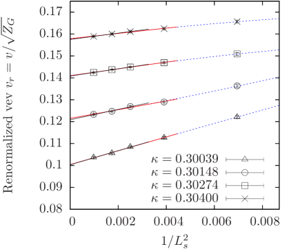 |
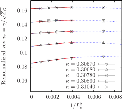 |
| (a) | (b) |
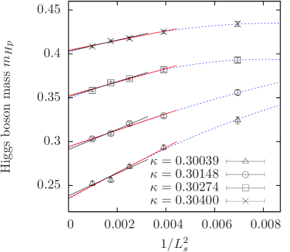 |
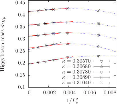 |
| (c) | (d) |
| Vacuum expectation value | ||||
|---|---|---|---|---|
| , | , | |||
| Higgs propagator mass | ||||
| , | , | |||
To obtain the desired upper Higgs boson mass bounds these finite volume results have to be extrapolated to the infinite volume limit and the renormalization factor has to be properly considered. For that purpose the finite volume dependence of the Monte-Carlo results on the renormalized vev and the Higgs boson mass , as obtained for the two scenarios of the full Higgs-Yukawa model and the pure -theory, is explicitly shown in Fig. 7.7. One sees in these plots that the finite volume effects are rather mild at the largest investigated hopping parameters corresponding to the lowest considered values of the cutoff , while the renormalized vev as well as the Higgs boson mass itself vary strongly with increasing lattice size at the smaller presented hopping parameters, as expected.
The aforementioned infinite volume extrapolation is then performed by applying the same strategy as in section 6.4.1. For that purpose the finite volume lattice data are fitted with the linear and the parabolic fit approaches given in Eq. (6.66) and Eq. (6.67), respectively. The resulting fits are displayed in Fig. 7.7. According to the smaller number of investigated lattice volumes as compared to the situation in section 6.4.1, only two different threshold values have been considered here. The respective fit parameters are listed in Tab. 7.6, where the presented final infinite volume results have been obtained by averaging over the parabolic fit and the two linear fits. Again, an additional systematic uncertainty is specified, which has been derived from the deviation between the latter fit results.
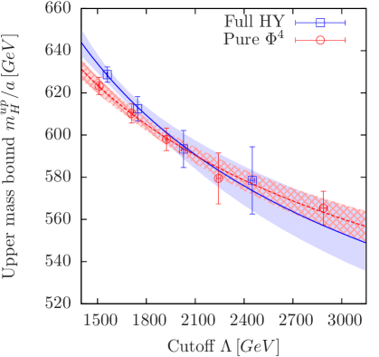 |
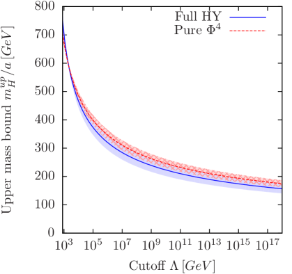 |
| (a) | (b) |
The sought-after cutoff dependent upper Higgs boson mass bound, and thus the main result of the current chapter, can then directly be obtained from the latter infinite volume extrapolation. The bounds arising in the full Higgs-Yukawa model and the pure -theory are jointly presented in Fig. 7.8a. In both cases one clearly observes the expected decrease of the upper Higgs boson mass bound with rising cutoff . Moreover, the obtained results can very well be fitted with the expected cutoff dependence given in Eq. (7.5), as depicted by the dashed and solid curves in Fig. 7.8a, where , are the respective free fit parameters.
Concerning the effect of the fermionic dynamics on the upper Higgs boson mass bound one finds in Fig. 7.8 that the individual results on the Higgs boson mass in the full Higgs-Yukawa model and the pure -theory at single cutoff values are not clearly distinguishable from each other with respect to the associated uncertainties. Respecting all presented data simultaneously by considering the aforementioned fit curves also does not lead to a much clearer picture, as can be observed in Fig. 7.8, where the uncertainties of the respective fit curves are indicated by the highlighted bands. At most, one can infer a mild suggestion from the presented results, being that the inclusion of the fermion dynamics causes a somewhat steeper descent of the upper Higgs boson mass bound with increasing cutoff . A definite answer regarding the latter effect, however, remains missing here due to the large statistical uncertainties. The clarification of this issue would require the consideration of higher statistics as well as the evaluation of more different lattice volumes to improve the reliability of the above infinite volume extrapolations.
On the basis of the latter fit results one can extrapolate the presented fit curves to very large values of the cutoff as illustrated in Fig. 7.8b. It is intriguing to compare these large cutoff extrapolations to the results arising from the consideration of the Landau pole presented in Fig. 1.1. One observes good agreement with that perturbatively obtained upper mass bound even though the here presented data have been calculated in the mass degenerate case and for . This, however, is not too surprising according to the observed relatively mild dependence of the upper mass bound on the fermion dynamics. For clarification it is remarked that a direct comparison between the aforementioned perturbative and numerical results is non-trivial due to the different underlying regularization schemes as already discussed in section 6.4.1. With growing values of , however, the cutoff dependence becomes less prominent, thus rendering such a direct comparison increasingly reasonable in that limit.
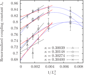 |
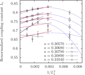 |
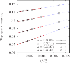 |
| (a) | (b) | (c) |
It is further remarked that the numerical determination of the presented cutoff dependence of the Higgs boson mass in physical units is rather demanding from a numerical point of view, since the vev as well as the mass both scale proportional to to lowest order in according to Eq. (7.2) and Eq. (7.3). This leading contribution thus cancels exactly when calculating the Higgs boson mass in physical units, i.e. , which would lead to a cutoff-independent Higgs boson mass, if only leading terms would be resolvable. It is only the subleading logarithmic contribution to the vev and the mass that yield the scaling behaviour presented in Eq. (7.5). The numerical data thus have to be precise enough to resolve the logarithmic contributions in order to observe the correct scaling behaviour. This is a demanding task from a numerical point of view, which could, however, satisfactorily be solved with relative errors being below the -level in the best cases thanks to the algorithmic improvements presented in chapter 5.
Finally, the question for the cutoff dependence of the renormalized quartic coupling constant and – in the case of the full Higgs-Yukawa model – the top quark mass with its associated value of the renormalized Yukawa coupling constant shall be addressed. For that purpose we follow exactly the same steps as above. The underlying finite volume lattice results on the renormalized quartic coupling constant and the top quark mass are fitted again with the parabolic and the linear fit approaches in Eq. (6.66) and Eq. (6.67) as presented in Fig. 7.9.
| Renormalized quartic coupling constant | ||||
| , | , | |||
| Top quark mass | ||||
| , | , | |||
The corresponding infinite volume extrapolations are listed in Tab. 7.7, where the final extrapolation result is obtained by averaging over all performed fit approaches, and an additional systematic error is again estimated from the deviations between the various fit procedures.
The sought-after cutoff dependence of the aforementioned renormalized coupling constants can then directly be obtained from the latter infinite volume extrapolations. The respective results are presented in Fig. 7.10 and one observes the renormalized coupling parameters to decrease with growing cutoff as expected in a trivial theory. Again, the obtained numerical results are fitted with the analytically expected scaling behaviour given in Eq. (7.6) and Eq. (7.7). As already discussed for the case of the Higgs boson mass determination, the individual measurements of in the two considered models at single cutoff values are not clearly distinguishable. Respecting the available data simultaneously by means of the aforementioned fit procedures also leads at most to the mild suggestion that the inclusion of the fermion dynamics results in a somewhat steeper descent of the renormalized quartic coupling constant with rising cutoff as compared to the pure -theory. A definite conclusion in this matter, however, cannot be drawn at this point due to the large statistical uncertainties encountered in Fig. 7.10.
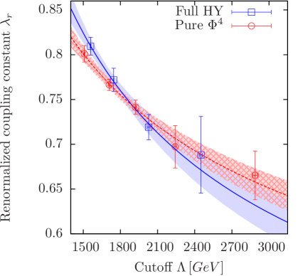 |
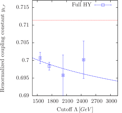 |
| (a) | (b) |
Furthermore, the renormalized Yukawa coupling constant is compared to its bare counterpart depicted by the horizontal line in Fig. 7.10b. Since the latter bare quantity was chosen according to the tree-level relation in Eq. (3.84) aiming at the reproduction of the physical top quark mass, one can directly infer from this presentation how much the actually measured top quark mass differs from its targeted value of . Here, one observes a significant discrepancy of up to , which can in principle be fixed in follow-up lattice calculations, if desired. According to the observed rather weak dependence of the upper Higgs boson mass bound on the Yukawa coupling constants, however, such an adjustment would most likely not even be resolvable with the here achieved accuracy. The same rationale also constitutes an additional reason why it was not tried to proceed to the investigation of the physically more relevant scenario of non-degenerate Yukawa coupling constants.
As a concluding remark it is summarized that the upper Higgs boson mass bound in the full Higgs-Yukawa model is very close to the one that arises in the pure -theory. With the here available statistics a difference between the latter two mass bounds could not clearly be resolved. It is only mildly suggested by the performed fit procedures that the descent of the upper Higgs boson mass bound with increasing cutoff may be somewhat steeper in the case of the full Higgs-Yukawa model than in the pure -theory. For a definite answer in this matter, however, higher statistics would be required.
Chapter 8 First results on the decay width of the Higgs boson
As a last consideration in the present work, only meant here as a brief and preliminary outlook towards some possible future developments that could be targeted in a further investigation of the underlying Higgs-Yukawa model, we will revisit the question for the decay properties of the Higgs boson in this chapter, having in mind that the determination of the decay width through the analysis of the Higgs propagator as presented in section 7.1.2 did not yield satisfactory results. For that purpose Lüscher’s well-known method [109, 110] for extracting the scattering phase shifts, and thus the decay width, from some finite volume lattice calculations shall be applied to the considered Higgs-Yukawa model. Subsequently, we will begin with a brief summary of the main concepts underlying the latter method, assuming the reader to be familiar with the basic theoretical background of scattering processes111An introduction to this subject can be found, for instance, in LABEL:Newton:2002zu,Taylor:2006zu. For the proofs and further details of Lüscher’s method the reader is referred to LABEL:Luscher:1990ux,Luscher:1991cf. in general.
To discuss the main ideas of Lüscher’s approach we first introduce an abstract system of two identical bosons with mass in a cubic box of continuous three-dimensional space with finite volume . Lüscher’s crucial observation has then been that the energy spectrum222Here and in the following we will only consider the center-of-mass frame, such that ’energy’ always means ’center-of-mass energy’ in this section. in the considered finite volume is connected to the scattering phase shifts of the two-boson system in infinite volume, where denotes the angular momentum quantum number. To elaborate more on the latter statement we introduce the center-of-mass energy of the two-boson system in the finite box . Moreover, the squared relative momentum in the center-of-mass frame is defined according to
| (8.1) |
It is remarked that this quantity is not restrained to the discrete set of finite volume momenta. In fact, is the relative momentum333With some abuse of notation the actual vector character of is omitted here. in the center-of-mass frame that one would observe for a given center-of-mass energy in the case of an infinitely large volume. This definition of the relative momentum has been established here, since the later given relation between and the scattering phase shifts actually connects with , i.e. the infinite volume scattering phase shifts at the relative momentum .
Furthermore, it is already emphasized at this point that the relations given in the following are only valid in the elastic scattering regime, that is for
| (8.2) |
The next crucial observation is that the announced relation between the scattering phase shifts and the observable energies is greatly restrained by symmetry arguments. For clarification we consider the eigenstate associated to a given energy eigenvalue . If is invariant under an adequately chosen representation of a symmetry group, one can directly exclude all those phase shifts from the announced relation to , the associated wave function of which, given in terms of the respective Legendre polynomials, is not invariant under the latter representation444For the here omitted details, the reader is referred to LABEL:Luscher:1990ux,Luscher:1991cf..
The symmetry group in the here considered scenario is the cubic group according to the continuous rotational symmetry being broken by the finite volume . The trivial representation of this group, which is denoted as , simply performs a discrete cubic rotation on a singlet wave function. As a consequence of the Legendre polynomials, more precisely the associated wave functions, being only invariant under for the phase shifts , , , , can not contribute to the energy , provided that the underlying state is invariant under . Similar statements can also be established for other representations of the considered symmetry group .
Moreover, it is a general result in scattering theory, known as threshold behaviour [203], that the phase shifts are suppressed at low momentum according to . Combining this general observation with the aforementioned exact symmetry constraints, one finds that the announced relation between and actually reduces to a relation between and with the next to leading order contribution given by at sufficiently small values of , provided that the underlying state is invariant under . Analogously, it would reduce to a relation between and , if was invariant under the vector representation , thus allowing to access also this scattering phase shift in a practical calculation, provided one can study the center-of-mass energies of states obeying that symmetry [197].
Here, however, we will only be interested in the scattering phase shift at zero angular momentum, i.e. . The corresponding relation to the energy has been worked out in detail in LABEL:Luscher:1990ux. For this scenario and up to the aforementioned corrections it is given as
| (8.3) | |||||
| (8.4) |
where is obtained for a given finite volume center-of-mass energy according to Eq. (8.1) and the function is defined555This relation defines only up to an integer multiple of . This ambiguity, however, is canceled in Eq. (8.3) by the modulo operation and is therefore ignored here. as
| (8.5) |
with denoting the zeta function according to
| (8.6) |
The physical interpretation of Eq. (8.3) is that the center-of-mass energies which are observable in a finite volume are constrained to a discrete set of energy values, determined by the condition that the respectively associated relative momentum solves the presented relation in Eq. (8.3) for a given infinite volume phase shift . Conversely, the given relation can be used to extract the aforementioned infinite volume scattering phase shift, once the energy levels observable in the finite volume are known, for instance by means of direct lattice calculations. It is pointed out, that the finite volume underlying such lattice calculations is not a disadvantage here that has to be overcome by some sort of infinite volume extrapolation. Instead, it is exactly the finiteness of the considered volume that is in fact exploited in Eq. (8.3) to derive the infinite volume scattering phase shifts in this approach. One has, however, to make sure that discretization effects are negligible in the intended lattice calculations, since the presented relations have been derived in the continuum.
It is further remarked that the definition of the zeta-function in Eq. (8.6) is only meaningful for sufficiently large real parts of , i.e. . At smaller real parts the zeta-function is instead defined through an analytic continuation of Eq. (8.6). For the calculation of its value at an integral representation has been devised in LABEL:Luscher:1990ux according to
which is well suited for a numerical evaluation. With the help of this expression it is straightforward to determine the phase shift according to Eq. (8.3) at the momenta determined through Eq. (8.1), once some center-of-mass energies have been computed for some finite volumes , such that the underlying states are invariant under the symmetry group representation . This is the strategy, mainly taken over from LABEL:Gockeler:1994rx, that will be applied in the following.
Before we continue, however, with the determination of the aforementioned energy levels , the question for the applicability of the discussed approach in the context of the here investigated Higgs-Yukawa model has to be addressed, since the above considerations were performed within a system of two identical bosons only, not respecting the existence of other particles such as the top and bottom quarks, for instance. However, the fermion dynamics can completely be integrated out, leading then to a solely bosonic system with a more complicated, effective coupling structure. Since no particular form of the underlying interaction has been assumed in LABEL:Luscher:1990ux for the derivation of Eq. (8.3), it thus follows that the so far given relations concerning the connection between the infinite volume scattering phase shifts and the bosonic, finite volume energy spectrum also hold in the considered Higgs-Yukawa model, respecting then also the fermionic contributions through the aforementioned effective coupling structure. In this picture the Goldstone bosons in the latter model can then be identified as the above introduced abstract bosonic particles with mass , while the Higgs boson would be considered as a resonance in that system [197].
It is further remarked that the so far stated relations have been obtained for the case of massive bosons, i.e. for . The Goldstone bosons in the considered Higgs-Yukawa model, however, would be massless. To overcome this problem, an external, space-time independent current is explicitly introduced into the Higgs-Yukawa model in the spirit discussed in section 2.1. The extended form of the bosonic action is then given as
| (8.8) |
where the latter current is assumed here and in the following to point into the 0-direction of the four component field . As a consequence the Goldstone bosons acquire a mass , thus finally establishing the applicability of the above discussed relations also for the case of the considered Higgs-Yukawa model.
For the purpose of determining the sought-after scattering phase shifts , and thus eventually also the width of the Higgs resonance, a series of lattice calculations has been performed with varying physical lattice volume as listed in Tab. 8.1. In these runs all model parameters were kept constant, while only the nominal number of lattice sites was varied, leading to an approximately constant physical scale and thus to a variation of the actual physical volume. The external current has been chosen such that the expected Higgs resonance mass lies in the elastic scattering region of the two Goldstone bosons according to Eq. (8.2), while the degenerate Yukawa coupling constants were again fixed by the tree-level relation in Eq. (3.84) aiming at the reproduction of the top quark mass.
| 0.13000 | 12 | 12 | 1 | 21440 | 0.01 | 0.36274 | 1.0 | 0.005 |
| 0.13000 | 16 | 16 | 1 | 20760 | 0.01 | 0.36274 | 1.0 | 0.005 |
| 0.13000 | 20 | 20 | 1 | 22100 | 0.01 | 0.36274 | 1.0 | 0.005 |
| 0.13000 | 24 | 24 | 1 | 10880 | 0.01 | 0.36274 | 1.0 | 0.005 |
| 0.13000 | 32 | 32 | 1 | 8780 | 0.01 | 0.36274 | 1.0 | 0.005 |
| 0.13000 | 36 | 36 | 1 | 4440 | 0.01 | 0.36274 | 1.0 | 0.005 |
| 0.13000 | 40 | 40 | 1 | 2360 | 0.01 | 0.36274 | 1.0 | 0.005 |
For clarification it is remarked that we start here with a rather small value of the bare quartic coupling constant in this exploratory study, which will later be seen to correspond to a renormalized quartic coupling constant of approximately , being around one order of magnitude smaller than for the case of the upper mass bound considered in section 7.3. The rationale behind this setting is that it allows for a direct comparison with renormalized perturbation theory in a regime where it can perfectly be trusted. Eventually, one is, however, rather interested in the case of the maximally possible renormalized quartic coupling constant, given at . The latter scenario would therefore be the prime target of some follow-up investigations.
The remaining step for the determination of the infinite volume scattering phase shift is thus the computation of the center-of-mass energies observable in the aforementioned finite volume calculations. Since we are here only interested in the zero angular momentum scatterings phase shift , we restrict the consideration to states which are invariant under the representation as discussed above. We therefore consider only correlation functions based on lattice observables , that obey the latter symmetry such as
| (8.9) | |||||
| (8.10) | |||||
| (8.11) | |||||
| (8.12) | |||||
| (8.13) |
where the set of lattice momenta is defined as
| (8.14) |
with denoting the unit vector pointing in direction and denotes here the number of elements of , i.e. . The operators in Eq. (8.9-8.13) would then generate states666When considering the given expressions in the operator formalism, their application to the vacuum generates a state , which is invariant under . As lattice observables they are invariant themselves under an appropriate representation of the symmetry group corresponding to . , that are invariant under . It is remarked here that the introduction of the external current explicitly breaks the original symmetry of the model. The 0-component of the field is now directly associated to the Higgs mode, while the other three components refer to the Goldstone modes. The given operators thus generate two particle states with isospin zero and relative lattice momentum as well as , respectively. It is further remarked that the operator only consists of a single field variable unlike the other operators. It is thus not directly a two particle operator. In fact, it directly corresponds to the expression given in Eq. (3.73), which was used to determine the Higgs boson mass in section 6.1.1. However, the states generated through have exactly the same quantum numbers as those resulting from the other introduced operators, such that can equally well be considered for our purpose.
We now define the time-slice correlation matrix according to
| (8.15) |
where adequate modulo operations are again implicit to guarantee . In the operator formalism one would then have
| (8.16) |
with
| (8.17) |
where has been assumed without loss of generality, is the, in this case non-degenerate, vacuum state, the index runs over all energy eigenstates of the underlying Hamiltonian except the vacuum state, denotes the associated energy eigenvalues, and is the counterpart of the lattice observable in the operator formalism. If one cuts off the infinite sum in Eq. (8.16) after the first summands, where the energy levels are assumed to be labeled in ascending order and only states with for at least one operator are counted, one obtains
| (8.18) |
with and the given diagonal matrix being -matrices here. This approximation is reasonable for sufficiently large values of and , which is assumed to be the case in the following. Subsequently, the given error term is therefore neglected.
If was unitary, the eigenvalues , of the hermitian correlation matrix would then directly be given as . Conversely, one could determine the energy eigenvalues by computing the eigenvalues of without picking up contaminations by lighter states. For a sufficiently large number of independent operators the low lying energy eigenvalues moreover become shielded against contaminations from excited states. The correlation matrix analysis would thus allow to extract these low lying energy eigenvalues as well as excited levels with very well controllable systematic effects.
The matrix , however, is not unitary in general, such that the eigenvalues of the hermitian correlation matrix are in fact some linear combinations of the exponentials listed above. The eigenvalues of can nevertheless be shown [204] to converge to the aforementioned exponential expressions for sufficiently large time separations , thus allowing to apply the above approach for the determination of the sought-after energy levels also in the general case, provided that sufficiently large time separations are considered.
Alternatively, the latter mixture can be resolved by studying the generalized correlation matrix instead of given as
| (8.19) | |||||
| (8.20) |
Provided that both error terms in Eq. (8.20) can be neglected, meaning that as well as are sufficiently large, the eigenvalues , of the generalized correlation matrix are given as , where is some reference time separation, thus directly allowing to read off the sought-after energy levels from the eigenvalues . This method is known in the literature as the generalized eigenvalue approach to the analysis of the correlation matrix [204].
Both approaches have been applied to the available data sets and it was found that the theoretically superior analysis based on the generalized correlation matrix in Eq. (8.19) leads here to larger statistic uncertainties of the extracted energy levels, rendering the determination of the sought-after decay properties of the Higgs boson less stable. For that reason, only the first analysis approach on the basis of the initial correlation matrix in Eq. (8.15) will be considered in the following.
Examples for the dependence of the eigenvalues on the time separation are presented in Fig. 8.1. The associated energy eigenvalues are here extracted by fitting the lattice data on each eigenvalue to the single -ansatz given in Eq. (6.2). For that purpose one has to assign the measured eigenvalues properly to each other, which can, for instance, be done by matching the respective eigenvectors.
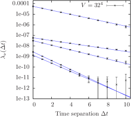 |
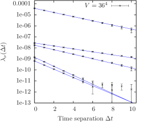 |
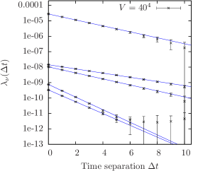 |
| (a) | (b) | (c) |
Analogously, the non-zero Goldstone mass is determined here by applying the above correlation matrix analysis also to the three Goldstone mode observables
| (8.21) |
where again the initial correlation matrix in Eq. (8.15) is considered due to the degeneracy of the Goldstone mass spectrum. The final numerical result on is then determined as the average over the resulting three degenerate Goldstone masses.
With the Goldstone mass777It is remarked that the Goldstone mass was found here to be independent of the lattice volume with respect to the achieved accuracy. and the energy eigenvalues at hand as observed in the performed finite volume lattice calculations, one can thus finally determine the scattering phase shifts at the associated momenta according to Eq. (8.1) and Eq. (8.3). For that purpose the consideration is restricted to only that part of the observed energy spectrum that lies within the elastic region specified by Eq. (8.2). The resulting scattering phase shifts are presented in Fig. 8.2. Since the phase shifts are only specified up to an integer multiple of , this freedom has explicitly been used to present the measured phase shifts in a monotonically increasing form.
In order to extract the Higgs resonance width from these numerical results on the scattering phase shifts, we will fit the latter data, more precisely the associated cross sections , with a Breit-Wigner function, which is a common approach for the description of resonance phenomena in general. Such an ansatz is, of course, not expected to describe the actual phase shifts exactly, which is why more elaborate fit approaches are used in other studies. Here, however, the achieved accuracy of the lattice data is not high enough to clearly resolve such differences. Moreover, the application of a Breit-Wigner fit provides a model-independent, general approach for the extraction of the decay width, not relying on any additional information, such as a perturbatively derived fit formula, for instance.
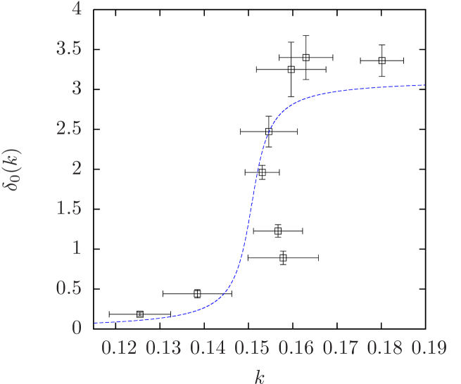
For that purpose the connection between the scattering phase shifts and the cross sections needs to be known. By virtue of the optical theorem [203] one has
| (8.22) | |||||
| (8.23) |
where all higher angular momentum contributions have been assumed to be negligible, which can again be justified according to the aforementioned threshold behaviour at sufficiently small momentum . As motivated above the resulting cross sections will then be fitted by a relativistic Breit-Wigner function given as
| (8.24) |
where the energy is related to the momentum by Eq. (8.1) and is not a free fit parameter but a function of , , and , which can easily be worked out such that and coincide at the resonance , where one has . The two free fit parameters in this approach are thus the Higgs resonance mass and its width . The fit curve obtained from this ansatz is presented in Fig. 8.2, while the underlying fit parameters, and thus the results on the resonance mass and width, are listed in Tab. 8.2.
| Resonance analysis | Reference value | |
|---|---|---|
| Mass | ||
| Decay width |
| observable | , | , | Final ext. result | |
| Final results of extrapolation in physical units | ||||
For clarification it is remarked that the resonance width as obtained through the above approach is given here as the full width of the Breit-Wigner function at half of its maximal height, which is commonly referred to as the FWHM-value in the literature. This definition of is somewhat arbitrary and does not exactly correspond [205] to the original definition of the Higgs decay width given through the location of the pole of the Higgs propagator continued onto the second Riemann sheet as specified in section 2.2. It can, however, be shown in the framework of some exactly solvable model [205] that these kinds of different definitions become equivalent in the limit of infinitesimally small decay widths. In the following we will therefore be ignorant towards a potential systematic discrepancy between the definitions of and .
At this point it would be interesting to compare these findings on the resonance width to some analytical expectations. Thanks to the relatively small value of the renormalized quartic self-coupling constant arising from the chosen setting , a reliable relation between the decay width , the renormalized coupling constant , the renormalized vacuum expectation value , and the boson masses and can be established by means of renormalized perturbation theory. For that purpose we reconsider the renormalized result on the Higgs propagator in Eq. (2.2), which has been established through a perturbative one-loop calculation in the pure -theory.
It has already been pointed out in section 2.2 that the given expression in Eq. (2.2) has to obey the minimal condition of being real for entirely real momenta , which directly constitutes the sought-after relation according to
| (8.25) |
where the definitions of and have been given in Eq. (2.36-2.37). This constraint has been solved numerically for the calculation of the spectral functions in Fig. 2.3. Here, however, an analytical approximation shall be presented. For that purpose we note that
| (8.26) | |||||
| (8.27) |
where the value in Eq. (8.27) arises from the branch cut of the arctanh-function in Eq. (2.31) and the minus sign originates from the continuation onto the second Riemann sheet. Combining the relations in Eq. (8.25-8.27) one directly finds the perturbative one-loop result for the sought-after relation in the pure -theory to be
| (8.28) |
where terms of order have been neglected and denotes the number of components of the scalar field , i.e. in our case. According to the here considered definition of the renormalized quartic coupling constant in Eq. (3.70), the latter expression becomes888The given result is identical to the formula applied in LABEL:Gockeler:1994rx.
| (8.29) |
where and have been identified with each other, which is justified here, since it only induces negligible corrections to being of order according to Eq. (3.69). The same substitution will also be exploited in the following.
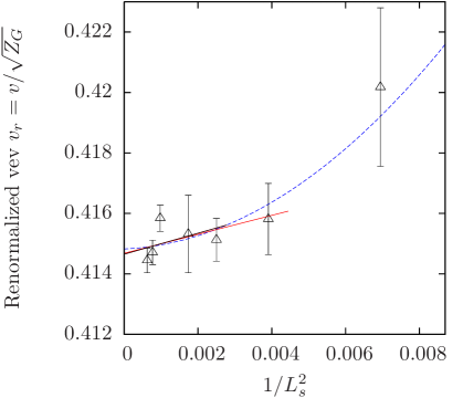 |
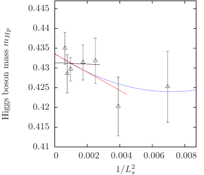 |
| (a) | (b) |
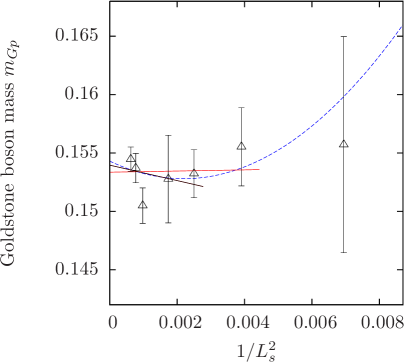 |
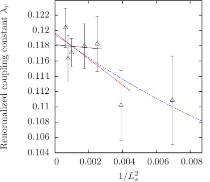 |
| (c) | (d) |
For the purpose of performing the aspired comparison with the perturbative calculation the infinite volume results on the renormalized quantities , , and need to be determined. This is done here in exactly the same manner as already detailed in section 7.3. The finite volume lattice data for the aforementioned quantities as well as for the renormalized vev are therefore presented in Fig. 8.3. These data are again plotted versus and fitted with the linear and parabolic fit approaches in Eq. (6.66) and Eq. (6.67). The resulting fit curves are also displayed in Fig. 8.3 and the underlying fit parameters are listed in Tab. 8.3, where the final infinite volume extrapolations are again determined as the respective average over all performed fit procedures.
With these data at hand the perturbative result on the decay width can be obtained from Eq. (8.29) as listed in Tab. 8.2. Comparing the results on and the Higgs propagator mass with the previously discussed resonance parameters and one observes satisfactory agreement with respect to the specified uncertainties.
As a concluding remark it is therefore summarized that the decay properties of the Higgs boson can indeed be determined in the considered Higgs-Yukawa model by virtue of Lüscher’s method [109, 110], even though the achieved accuracy and thus the underlying statistics of generated field configurations certainly has to be increased in follow-up investigations. At this point, however, only a preliminary and brief outlook has been given on what could be done next. In particular, the quartic coupling constant has here been fixed to a rather small value to allow for a reliable comparison with perturbation theory. In a follow-up investigation one could be interested in increasing the underlying renormalized quartic coupling constant up to its maximal value by sending the bare parameter to infinity, which would eventually allow to study the maximally possible decay width of the Higgs boson in the here considered Higgs-Yukawa model.
Chapter 9 Summary and conclusions
The aim of the present work has been the non-perturbative determination of the upper and lower mass bounds of the Standard Model Higgs boson based on first principle computations, in particular not relying on additional information such as the triviality property of the Higgs-Yukawa sector or indirect arguments like vacuum stability considerations. The motivation for the consideration of the aforementioned mass bounds finally lies in the ability to draw conclusions on the energy scale at which a new, so far unspecified theory of elementary particles definitely has to substitute the Standard Model, once the Higgs boson and its mass will have been discovered experimentally. In that case the latter scale can be deduced by requiring consistency between the observed mass and the mass bounds and intrinsically arising from the Standard Model under the assumption of being valid up to the cutoff scale .
The Higgs boson might, however, very well not exist at all, especially since the Higgs sector, can only be considered as an effective theory of some so far undiscovered, extended theory, due to its triviality property. In such a scenario, a conclusion about the validity of the Standard Model can nevertheless be drawn, since the non-observation of the Higgs boson at the LHC would eventually exclude its existence at energies below, lets say, thanks to the large accessible energy scales at the LHC. An even heavier Higgs boson is, however, definitely excluded without the Standard Model becoming inconsistent with itself according to the results in chapter 7 and the requirement that the cutoff be clearly larger than the mass spectrum described by that theory. In the case of non-observing the Higgs boson at the LHC, one can thus conclude on the basis of the latter results, that new physics must set in already at the TeV-scale. For the rest of this section, however, we assume the discovery of the Higgs boson with mass allowing then to draw conclusions on in the previously described manner.
For the purpose of establishing the aforementioned mass bounds, the lattice approach has been employed to allow for a non-perturbative investigation of a Higgs-Yukawa model serving here as a reasonable simplification of the full Standard Model, containing only those fields and interactions which are most essential for the Higgs boson mass determination. The model therefore consists of the scalar field , composed out of the Higgs and the Goldstone modes, as well as the top-bottom doublet and their mutual interactions, which together are responsible for the emergence of the lower Higgs boson mass bound. Moreover, the considered Higgs-Yukawa model also describes the self-interaction of the scalar field , which is expected to yield the largest contribution to the upper Higgs boson mass bound as the bare quartic coupling constant is sent to infinity, thus motivating the non-perturbative approach.
According to the chiral nature of the electroweak interaction in the full Standard Model, left- and right-handed particles couple differently among each other. To maintain this chiral gauge coupling structure also on the lattice a consistent formulation of chiral gauge theories on the lattice would be required. Due to the neglection of any gauge fields in the here considered Higgs-Yukawa model, however, the latter local gauge symmetry reduces to a global symmetry, which can then be realized on the lattice by virtue of Lüscher’s proposals in LABEL:Luscher:1998pq.
In the present work the aforementioned proposal for the construction of chirally invariant lattice Higgs-Yukawa models has been applied to the situation of the actual Standard Model Higgs-fermion coupling structure, i.e. for being a complex doublet equivalent to one Higgs and three Goldstone modes. The resulting chirally invariant lattice Higgs-Yukawa model, constructed here on the basis of the Neuberger overlap operator, then obeys a global symmetry, as desired.
The fundamental strategy underlying the determination of the cutoff-dependent upper and lower Higgs boson mass bounds has then been the numerical evaluation of the maximal interval of Higgs boson masses attainable within the considered Higgs-Yukawa model in consistency with phenomenology. The latter condition refers here to the requirement of reproducing the phenomenologically known values of the top and bottom quark masses as well as the renormalized vacuum expectation value of the scalar field, where the latter condition was used here to fix the physical scale of the performed lattice calculations. Applying this strategy thus requires the evaluation of the model to be performed in the broken phase, however close to a second order phase transition to a symmetric phase, in order to allow for the adjustment of arbitrarily large cutoff scales, at least from a conceptual point of view.
As a preparatory consideration the phase structure of the underlying Higgs-Yukawa model has therefore been investigated, which has been done here in the limit of an infinite number of degenerate fermion generations. Though the actual physical situation in the Standard Model corresponds to the finite and even small setting , or rather to respect also the colour index despite the general absence of the gauge fields themselves, it was still possible to derive the qualitative phase structure of the Higgs-Yukawa model by means of this approach. The considered order parameters have been chosen to be the vacuum expectation value as well as its staggered counterpart which finally allowed to locate the symmetric (, ) and the broken (, ) phases of the model in bare parameter space. In fact, a rich phase structure could be observed including also phases with and as well as phases with and , where the vacuum expectation values and are simultaneously non-zero.
This investigation of the phase structure in the large -limit has primarily targeted the scenario of small Yukawa coupling constants, since this is the relevant setup for the considered purpose. However, the model has also been studied in the limit of large Yukawa coupling constants. Interestingly, a symmetric phase also emerges in this scenario, the existence of which, however, is obscured by strong finite volume effects, hindering its observation on too small lattices. Though this part of the phase structure is not of direct interest for the present study, it seems to be valuable for other questions, such as the study of mass generation in this strong coupling symmetric phase [103] or the investigation of nucleon bound states induced by pion exchange, which is assumed to be describable by means of a Higgs-Yukawa model with strong Yukawa coupling constants [206], however with a very different interpretation of the underlying field content. In both cases, i.e. for small as well as for large Yukawa coupling constants, the phase transitions between the symmetric and the broken phase were found to be of second order, making the model thus suitable for direct lattice calculations. To confirm the validity of the performed analytical calculations, the above results have explicitly been compared to direct Monte-Carlo computations at finite values of and good agreement has been observed.
With this information about the second order phase transition line between the symmetric and broken phases at hand, the next step towards the aim of the present study has been the preparation of a suitable simulation algorithm, capable of evaluating the considered model for arbitrary, especially for odd values of . For that purpose a PHMC algorithm [108] has been implemented. This underlying concept, however, has been extended by a number of algorithmic improvements applicable at least in the case of the here considered Higgs-Yukawa model, which finally led to a substantial and indispensable performance gain. Among them are a preconditioning technique, reducing the condition number of the underlying fermion operator by 1-2 orders of magnitude, the well-known Fourier acceleration approach finally resulting in drastically smaller auto-correlation times, as well as an exact, Krylov-space based reweighting strategy allowing to further reduce the degree of the employed approximation polynomials while keeping the algorithm exact. Some of these techniques, for instance the latter reweighting strategy, can directly be applied also to the case of QCD, while others are not directly adaptable, as discussed in chapter 5. In total, the presented enhancements induced a very substantial performance gain which was crucial for the success of the performed lattice calculations.
Equipped with these technical and conceptual preparations the question for the lower Higgs boson mass bound could finally be addressed. For that purpose it has explicitly been confirmed by direct lattice calculations that the lightest Higgs boson masses are indeed generated at vanishing quartic self-coupling constant, as suggested by analytical calculations performed in the framework of the constraint effective potential, thus allowing to restrict the search for the lower Higgs boson mass bound to the scenario of . For the mass degenerate case with equal top and bottom quark masses and the finite volume lattice results on the Higgs boson mass obtained at for a series of cutoffs and lattice sizes have then been presented and compared to their respective analytical predictions based on the aforementioned effective potential calculations and very good agreement has been observed. These numerical finite size results were then extrapolated to the infinite volume limit to actually establish the desired cutoff-dependent lower Higgs boson mass bound , as summarized in Fig. 9.1.
The main effort concerning the investigation of the lower bound has been spent on the above mentioned degenerate scenario with and , since it is reliably accessible from a numerical as well as from a conceptual point of view. This situation changes when one proceeds to the physically more relevant case of and non-degenerate Yukawa coupling constants fixed according to the phenomenologically known values of the top and bottom quark masses. In that scenario one becomes confronted with the conceptual problem of a fluctuating complex phase of the fermion determinant leading to unknown systematic uncertainties on the numerical results arising from the employed simulation algorithm. In addition, the numerical requirements themselves are also significantly increased in this parameter setup according to larger condition numbers of the fermion matrix as well as stronger finite volume effects induced by the large ratio of the bottom and top quark masses. The numerical investigation of the lower Higgs boson mass bound has nevertheless been tried also in this scenario and the obtained results are in agreement with the analytical prediction arising from the aforementioned effective potential calculation, though a clear resolution of the differences between the considered degenerate results and the non-degenerate results could not be achieved. However, assuming the latter effective potential calculations to remain trustworthy also in the non-degenerate scenario, which is in agreement with the observed lattice results, one would then find a cutoff-dependent lower Higgs boson mass bound of approximately at a cutoff scale of , as summarized in Fig. 9.1.
The main result of the presented findings is that a lower Higgs boson mass bound is a manifest property of the pure Higgs-Yukawa sector that evolves directly from the Higgs-fermion interaction for a given set of Yukawa coupling constants. With growing cutoff this lower mass constraint was found to rise monotonically with flattening slope as expected from perturbation theory. Moreover, the quantitative size of the obtained lower bound is comparable to the magnitude of the perturbative results based on vacuum stability considerations [71] as presented in Fig. 1.1. A direct quantitative comparison between the latter approaches is, however, non-trivial due to the different underlying regularization schemes in combination with the strong cutoff-dependence of the considered constraints.
The question for the universality of the derived lower mass bound has then briefly been addressed by studying its dependence on the extension of the underlying Lagrangian by some higher order self-interaction terms of the scalar field, i.e. and in this case. Such a consideration is not excluded by the usual renormalization arguments, since the Higgs-Yukawa sector can only be considered as an effective theory due to its triviality property. With the help of adequate analytical calculations in the framework of the constraint effective potential, several bare parameter setups have been estimated for this extended model, which supposedly lead to Higgs boson masses undercutting the lower mass bounds previously established in the pure Higgs-Yukawa model. By means of direct lattice Monte-Carlo computations it could then be shown, that the selected parameter setups indeed generate Higgs boson masses which are significantly pushed below the aforementioned lower bound. The interpretation of this finding is that the lower Higgs boson mass bound arising in the pure Higgs-Yukawa model cannot be considered as being universal, i.e. it is not independent of the specific form of the underlying interactions. However, the Higgs boson mass could not be made arbitrarily small, though the aforementioned effective potential calculations would have suggested that. This might be an indication for the existence of a true lower bound also in this extended scenario. It might, however, also be that only the applied method for finding adequate bare coupling parameters in this extended model, which would potentially lead to even smaller Higgs boson masses, has to be further improved. Moreover, one may ask whether smaller masses can be attained by including even more coupling terms within the Lagrangian. This issue poses an interesting problem for future investigations.
The question for the upper Higgs boson mass bound has then been addressed by applying the same conceptual strategy also in the regime of large quartic self-coupling constants . In a first step it has explicitly been confirmed by direct lattice calculations that the largest attainable Higgs boson masses are indeed observed in the case of an infinite bare quartic coupling constant, as suggested by the aforementioned effective potential calculations. Consequently, the search for the upper Higgs boson mass bound has subsequently been constrained to the bare parameter setting . The resulting finite volume lattice data on the Higgs boson mass turned out to be sufficiently precise to allow for their reliable infinite volume extrapolation, yielding then a cutoff-dependent upper bound of approximately at a cutoff of . These results were moreover precise enough to actually resolve their cutoff-dependence as summarized in Fig. 9.1, which is in very good agreement with the analytically expected logarithmic decline, and thus with the triviality picture of the Higgs-Yukawa sector. It is pointed out again, that this achievement has been numerically demanding, since the latter logarithmic decline of the upper bound is actually only induced by subleading logarithmic contributions to the scaling behaviour of the considered model close to its phase transition, which had to be resolved with sufficient accuracy. By virtue of the analytically expected functional form of the cutoff-dependent upper mass bound, which was used here to fit the obtained numerical data, an extrapolation of the latter results to much higher energy scales could also be established, being again in good agreement with the corresponding perturbatively obtained bounds [71] presented in Fig. 1.1. A direct comparison has, however, again been avoided here for the previously discussed reasons.
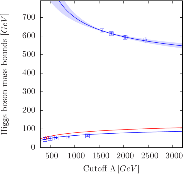
The interesting question for the fermionic contribution to the observed upper Higgs boson mass bound has then been addressed by explicitly comparing the latter findings to the corresponding results arising in the pure -theory. For the considered energy scales this potential effect, however, turned out to be not very well resolvable with the available accuracy of the lattice data. The performed fits with the expected analytical form of the cutoff-dependence only mildly suggest the upper mass bound in the full Higgs-Yukawa model to decline somewhat steeper with growing cutoffs than the corresponding results in the pure -theory. To obtain a clearer picture in this respect, a higher accuracy of the numerical data and thus a higher statistics of the underlying field configurations would be needed.
It has moreover also been tried to derive some first information on the decay properties of the Higgs boson directly from the analysis of the curvature of the Higgs propagator based on its renormalized perturbative one-loop expression, which was analytically derived in continuous Euclidean space-time. This approach, however, turned out to be not successful in the here considered scenarios of large quartic coupling constants, since it was not possible to stabilize the corresponding fit result on the decay width , meaning here to retrieve results on independently of the momentum interval in which the propagator has been analyzed. In that respect it might be interesting to ask, whether this problem can be overcome by considering perturbative calculations of the Higgs propagator up to higher orders in the renormalized quartic coupling constant and including also the fermionic contributions, while simultaneously increasing the underlying statistics of field configurations.
In the present work, however, this ansatz has not further been pursued. Instead, a first account on Lüscher’s method [109, 110] for determining the Higgs boson decay width by studying the volume dependence of the finite size lattice mass spectrum has been given. This brief and preliminary outlook was only meant here as a conceptual study, demonstrating the applicability of the latter method in the framework of the considered Higgs-Yukawa model. For that purpose a model parameter setup associated to a rather small renormalized quartic self-coupling constant has been chosen, since this allowed to derive a reliable reference value for the Higgs boson decay width from perturbation theory. In the subsequent analysis it was then found that the Higgs boson decay width can indeed be determined with the help of Lüscher’s approach in the here considered Higgs-Yukawa model. The observed numerical value for was moreover found to be in agreement with the corresponding result derived from a perturbative one-loop calculation in the pure -theory, thus encouraging to repeat similar analyses also in the physically more interesting scenario of maximal values for the renormalized quartic self-coupling constant, i.e. at . This will then eventually allow to establish an upper bound also for the decay width of the Standard Model Higgs boson on the basis of the here considered Higgs-Yukawa model.
Such future extensions of the here presented investigation can directly be pursued with the already implemented software code. In this respect one might, however, want to improve the applied analysis by considering the so-called moving-frame, referring here to the frame, relative to which the involved momenta and energies are determined. Concerning the relatively large observed statistical uncertainties in chapter 8 one would also want to significantly increase the underlying statistics of field configurations. By virtue of the algorithmic improvements presented in chapter 5 and according to the applied parallelization technique discussed in appendix B this can directly be achieved by simultaneously rerunning multiple replicas of the lattice calculations considered in chapter 8. With such an ansatz it is apparently possible to increase the field configuration statistics, at least for some small number of selected runs, by clearly more than one order of magnitude111This is one of the projects initiated and pursued by Jim Kallarackal.. This should then allow to study the Higgs boson decay properties with higher precision. It should moreover allow to clearly identify the fermionic contributions to the upper Higgs boson mass bound.
In addition to that it might be worthwhile to repeat the presented Higgs propagator analyses presented in sections 6.1.3 and 7.1.2 on the basis of some improved analytical fit formula, including also higher order and in particular fermionic contributions, which might then, together with the aforementioned significantly increased statistics, allow to extract some decay properties also from this approach.
Appendix A The Lanczos method for computing
In LABEL:Borici:1999ws a Lanczos-based, iterative method was presented, capable of computing for a given positive, hermitian matrix and a given vector . Its main idea is to approximate by the inverse square root of the projection of the operator onto the Krylov space
| (A.1) |
for some sufficiently large value of . In this section the latter method shall be extended to the more general case of computing , where is a given real function111The function is a real function acting on real numbers. With some abuse of notation, however, it will also be applied to hermitian matrices in the sense that it actually acts on their respective eigenvalues in the spectral representation. with , . For clarification it is remarked that the subsequent discussion, which is based here on the latter general operator , directly includes also the special case of , which is actually of interest in the present work.
Here, we begin with the discussion of the original version of the aforementioned Lanczos-based algorithm as specified in LABEL:Borici:1999ws. For a given prescribed relative accuracy it iteratively generates a sequence of orthonormal vectors by the successive application of the operator , starting from . The number of Lanczos iterations specifies the total of performed matrix applications of the considered operator . The vectors then form an orthonormal basis of . Moreover, the Lanczos algorithm generates a tridiagonal -matrix , which is by construction the representation of the operator projected onto the Krylov space in the basis . In detail this algorithm reads [188]:
| (A.2) | |||
| end for |
The aforementioned tridiagonal matrix is then defined on the basis of the computed values and according to
| (A.7) |
where the above indices of the matrix take the values . The approximation for is then given as
| (A.8) |
where is the problem size, i.e. the size of the vector , and denotes the unit vector with length in 0-direction, according to , . The inverse square root of the -matrix , which is well defined since the matrix is symmetric and positive by construction, can then be computed by a spectral decomposition of in terms of its eigenvalues and eigenvectors, which are, for instance, obtainable with the help of some standard linear algebra software package [163] due to the typically small size of the problem and the tridiagonal form of .
In principle, the above approach can be applied to any function by replacing the inverse square root in Eq. (A.8) with that general function. The vital questions are, whether the expression in Eq. (A.8) then still converges and - from a more pragmatic point of view - whether one has a reliable and practical stopping criterion at hand indicating the actually achieved relative accuracy, that has been reached after a certain number of Lanczos iterations, to be below the prescribed value . Here, the notion ’practical’ refers to the numerical costs of that criterion, since a direct test would always be possible, at least in principle.
For the case of the inverse square root, i.e. for with such a stopping criterion has been devised in LABEL:Borici:1999ws as presented in Eq. (A.2). In fact, the given condition is just the standard CG-stopping criterion222Up to finite machine precision rounding errors which are, however, ignored here and in the following. [188, 144], which guarantees the residual
| (A.9) |
of a corresponding CG-process [127] for applying the inverse of to after iterations to be bounded by
| (A.10) |
The main statement of LABEL:Borici:1999ws, which was proven in LABEL:vandenEshof:2002ms, is that the latter CG-stopping criterion is inherited also to the case of the inverse square root.
Here, one further step shall be taken. It will be shown in the following that the same condition given in Eq. (A.2) can also be exploited to monitor and proof the convergence of
| (A.11) |
provided that the real, non-zero function can be written in the form
| (A.12) |
Examples of functions lying in this class will be given later. For now we continue with the proof, which is just an extension of the one originally given in LABEL:vandenEshof:2002ms. For that purpose we define the generalized residuals333The definition of the generalized residuals in Eq. (A.13) becomes identical to Eq. (A.9) for .
| (A.13) |
where is some non-negative real number, is the identity acting on the same space as , and is the identity matrix. In the following we will need the explicit relation [144] between and given as
| (A.14) |
where denotes the eigenvalue of . The above relation directly follows from the representation [207] of the generalized residuals according to
| (A.15) |
which is given here in terms of the so-called Lanczos polynomials [207] defined as
| (A.16) |
such that is a polynomial of degree . With this preparation at hand one finds in particular that , since is positive and .
The actually relevant residual, which will be considered here to prove the convergence of Eq. (A.11), is defined as
| (A.17) |
The sought-after proof can then be established through
| (A.18) | |||||
| (A.19) | |||||
| (A.20) |
where the operator is defined as
| (A.21) |
The missing link for arriving at Eq. (A.20) is to show that the operator norm is bounded from above by one, i.e. , where the latter supremum is performed over all vectors . For that purpose let be an arbitrary eigenvalue of with associated eigenvector . Exploiting the requirements and specified in Eq. (A.12) as well as the aforementioned relation , one directly finds
| (A.22) | |||||
| (A.23) |
which proofs and thus Eq. (A.20). Under the assumption that the standard CG-algorithm converges for the given matrix and the vector we have now shown that the approximation in Eq. (A.11) also converges and that the standard CG-stopping criterion given in Eq. (A.2) guarantees the relative error to be smaller than , provided that the considered function can be written in the form of Eq. (A.12). This is indeed the case for the inverse square root according to the integral representation
which was used in Refs. [188, 144]. Besides this particular case, the required preconditions are also fulfilled for arbitrary inverse roots, i.e. , according to the more general integral identity
| (A.24) |
which was obtained here with the help of some computer algebra system [126]. Combining this Lanczos-based method with direct applications of the operator and its inverse , computable by the standard CG-algorithm, one can thus calculate for any function of the form , as announced.
Finally, an example for the convergence of this approach shall be given. For that purpose we consider a test setup consisting of three different functions , given as
| (A.25) | |||||
| (A.26) | |||||
| (A.27) |
where the first case corresponds to the standard case of a matrix inversion computable by the usual CG-algorithm, the second example refers to the calculation of the inverse square root as proposed in LABEL:Borici:1999ws, and the third case belongs to the extended scenario discussed above. For the purpose of determining the achieved relative accuracy the following measure
| (A.28) |
is introduced. In Fig. A.1a the dependence of the latter relative accuracy on the number of performed Lanczos iterations is presented for the three considered test cases. These results have been obtained for the particular case , which is actually relevant for this study. Here, however, the unpreconditioned version of the fermion matrix according to its original definition in Eq. (3.47) has been applied. The underlying lattice volume was chosen to be , the degenerate Yukawa coupling constants were set to , and the scalar field appearing within the operator as well as the pseudo fermion vector were both randomly sampled according to a standard Gauss distribution. The presented data then display the results obtained in a single inversion process starting with identical field configurations and in each considered test case.
For the scenario at sufficiently large values of it is well known that the relative deviation will finally vanish exponentially with the number of performed Lanczos iterations . Before this asymptotic behaviour sets in, however, the relative deviation is not expected to decrease monotonically. This is clearly seen in Fig. A.1a. Moreover, one also observes in that presentation that the relative deviations , for the other two test cases are bounded by , as demonstrated above.
In Fig. A.1b the achieved relative accuracies are presented versus the prescribed relative accuracy specified through . For the case this approximately yields a straight line with slope of one, since the estimate for the norm of the residual in Eq. (A.2) is exact in this scenario and . In the two other cases the actually obtained relative accuracy is a more complicated function of with the very essential condition, however, that one always has , as proven above.
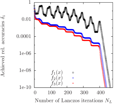 |
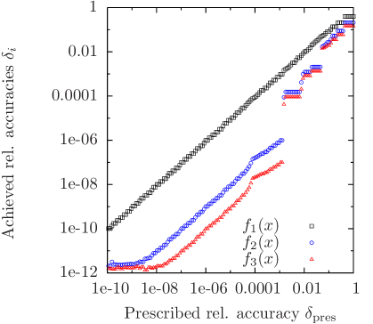 |
| (a) | (b) |
Appendix B Fast implementations of FFT in four dimensions
According to the absence of gauge fields in the here considered Higgs-Yukawa model the Dirac operator can very efficiently be constructed in momentum space as discussed in section 3.5. Since the operator in Eq. (3.49), on the other hand, is local in position space, the aforementioned strategy requires the pseudo fermion vector to be transformed from position to momentum space or vice versa each time one of the operators and , respectively, is applied to . It is well known that this can very efficiently be done by means of a Fast Fourier Transform111The notion ’Fourier transform’ will always refer to a discrete Fourier transform of a vector or a multi-dimensional array of complex numbers in this section. (FFT), the numerical complexity of which being of order . Since the complexity class of applying the latter operators and is only of order according to their respective diagonal structure, the aforementioned Fourier transformations thus constitute the limiting factor of a practical implementation of the considered computation strategy with respect to the overall numerical performance in the limit of large lattice volumes.
The availability of an efficient software code for performing Fast Fourier Transformations on an actually given computer hardware is therefore of significant importance for the success of the above computation strategy in practice. In this section some remarks on the technical details concerning such software implementations shall therefore be given, including also the here applied form of their parallelization.
As a first step we begin with the consideration of a one-dimensional Fourier transform of the complex vector with the index running from to . Neglecting any normalization constants the Fourier transform of is here defined as
| (B.1) |
Implementing this formula exactly as written would then lead to an algorithm lying in the complexity class , thus rendering its application in a practical approach unfeasible. The well known cure to this problem is the Fast Fourier Transform. In fact, the notion ’Fast Fourier Transform’ does not refer to one specific algorithm but rather to a whole class of algorithms that can compute Eq. (B.1) with a numerical complexity of order . The probably most widely known approach is the (radix-2) Cooley-Tukey algorithm [208]. In case of being a power of , which shall always be assumed in the following, it computes according to222 is defined through Eq. (B.3), while Eq. (B) only holds for .
| (B.2) | |||||
| (B.3) | |||||
through the recursive formula
for and else
| (B.6) |
Computing this recursive algorithm literally as described above would again lead to the numerical expenses being of order . The crucial observation, however, is that
| (B.7) |
such that the quantity only needs to be computed for . If one further exploits for and one finds that a total number of
| (B.8) |
real additions and
| (B.9) |
real multiplications are required for the here presented Cooley-Tukey algorithm. For clarification it is remarked that a single complex multiplication translates into four real multiplications plus two real additions. Moreover, trivial multiplications, i.e. multiplications with or , have been counted here as full multiplications. However, the given recursive formulation, though very helpful for the mathematical analysis of the underlying numerical operations, is usually not directly employed for the practical implementation of the algorithm. For that purpose some more effort has to be invested into an appropriate bookkeeping of the computed interim results . A very convenient approach is based on the reordering of the start vector according to such that is the bit-reversal of the binary representation of the number in the binary number system. These details, however, shall not be discussed here333A basic introduction to the implementation of the Cooley-Tukey algorithm can, for instance, be found in LABEL:Press:2007zu. An advanced approach is presented in LABEL:Burrus:2009zu..
As already pointed out above, the (radix-2) Cooley-Tukey approach is only one variant of a FFT algorithm. In fact, there are other methods, for instance split-radix algorithms [210, 211] and even more efficient variations thereof [212], requiring at least less floating point operations, while still belonging to the same complexity class . Since the aforementioned number of floating point operations counts all performed real multiplications plus the additions, one would thus expect these more elaborate algorithms to be clearly superior to the Cooley-Tukey approach in terms of required runtime, i.e. the time needed to perform a specific FFT.
This, however, is not necessarily the case in practice. The reason is that the true runtime speed of a certain software code on a given hardware depends on many more variables than just the total number of required elementary operations and the clock-speed of the processor in terms of operations per time. Among these factors are, for instance, the achieved level of cache coherence and data locality, as discussed later in this section.
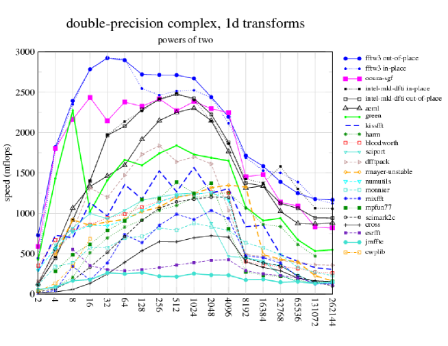
According to the large variety of hardware platforms it is therefore very difficult to devise a particular algorithm that is optimal for all underlying hardware architectures. A tremendous collection of various FFT algorithms and corresponding software realizations thereof has therefore been implemented and assembled into a single software library known as the ’Fasted Fourier Transform in the West’ (FFTW) [155], such that the library automatically picks that software code that runs most efficiently on the respective hardware architecture. This selection procedure will be referred to in the following as the internal FFTW tuning process.
In Fig. B.1, which was taken from the FFTW homepage [213], the performance of the FFTW library is compared to the corresponding runtime speeds of other publicly available FFT implementations, as detailed in LABEL:FFTWHomepage. The here specified MFLOPS-numbers (million floating point operations per second) have been determined according to
| MFLOPS | (B.10) |
where denotes here the number of micro seconds that the respective implementation needed to perform the Fast Fourier Transform of the one-dimensional complex vector with vector length . For clarification it is remarked that this quantity does not give the correct number of floating point operations that the respective algorithm actually performed. In fact, the factor is just a reasonable normalization of the measured time , which is, however, motivated by the number of floating point operations that the above presented Cooley-Tukey approach would have required444Apart from the aforementioned unnecessary counting of trivial multiplications..
From this presentation one can infer that the FFTW library indeed provides the fastest one-dimensional, complex FFT implementation among all here considered competing software codes. However, one also learns from Fig. B.1 that the achieved numerical performance significantly decreases with growing vector length due to a reduction of the underlying cache coherency and data locality, as will later be discussed in this section.
Concerning the technical details of this comparison the underlying hardware architecture has been a Dual Core AMD Opteron(tm) Processor 275, 2.2 GHz, 64 bit mode as further specified in LABEL:FFTWHomepage and the transformed complex vector has been represented in double precision, i.e. with 64 bit per real number. This setup has been chosen among the various speed monitorings available in LABEL:FFTWHomepage, since it comes closest to the scenario of the lattice calculations considered in the context of this work, which have mainly been performed on the HP XC4000 System [214] at the Scientific Supercomputing Center Karlsruhe, built on the basis of AMD Opteron(tm) Processors, however with a higher clock-speed of . Though the hardware architecture actually underlying the HP XC4000 System is not exactly identical to the one tested above, it is nevertheless reasonable to assume the FFTW library to provide the most efficient one-dimensional FFT implementation also on that machine.
For the purpose of this study, however, we are mainly interested in four-dimensional Fourier transforms. More precisely, it is the complex pseudo fermion field that needs to be transformed with denoting the four-dimensional lattice site index and , being the inner spinor index associated to the fermion doublets. This multi-dimensional Fourier transform can, however, trivially be decomposed into a series of one-dimensional Fourier transforms computed along each respective space-time axis according to
| (B.11) |
where denotes the lattice size in direction and all global normalization factors have again be discarded for simplicity. The FFTW library, however, directly comes along with routines automatically exploiting and optimizing this decomposition scheme internally. The resulting MFLOPS-rates as observed for a typical test case with and the lattice side lengths being a power of two are presented in Fig. B.2a, where the presented MFLOPS-rates have here been determined according to
| MFLOPS | (B.12) |
with being the lattice volume and denoting the execution time in micro seconds. Again, this quantity does not give the exact number of floating point operations actually performed, but it is motivated by the operation count of the multi-dimensional Cooley-Tukey algorithm in the previously described sense. It is further remarked that the presented MFLOPS-rates have directly been obtained on the aforementioned HP XC4000 System with version 3.2.2 of the FFTW library, since no four-dimensional performance tests were available on the FFTW homepage [213] at the time this work has been compiled.
As expected one observes in Fig. B.2a that the numerical performance of the FFTW implementation significantly decreases with growing lattice volume. On the largest presented volumes one moreover finds it to be of similar magnitude, even somewhat larger than the results in Fig. B.1, when mapping the respective one-dimensional and four-dimensional volumes adequately to each other, while also respecting the higher clock-speed of as compared to the underlying the measurements in Fig. B.1.
It is remarked that the notions ’fully tuned’ and ’partly tuned’ appearing in the legend of Fig. B.2 refer to the set of FFT implementations that are actually considered inside the FFTW library for the internal optimization procedure. In the fully tuned case, associated to the optimization mode FFTW_MEASURE | FFTW_EXHAUSTIVE in LABEL:FFTW05, the system explicitly and individually measures the true wall clock runtime for all available FFT implementations contained in the FFTW library and selects then the actually fastest code. In the other case, referred to as ’partly tuned’, which is specified through the flag setting FFTW_MEASURE, this optimization is restricted to a certain subset of these implementations, resulting then in a reduced amount of time required by the optimization process. From the comparison in Fig. B.2a one infers that the performance of the partly tuned approach is almost identical to that of the fully tuned FFTW code in the example presented here. In the following we will nevertheless always consider the fully tuned approach with the intention to obtain the optimal performance out of the FFTW routines.
However, it turns out that the achieved performance of the already very efficient FFTW implementation of the four-dimensional complex Fourier transform can be pushed to an even higher level at least in the here considered setup which, however, is typical for the needs of this study. For that purpose a new implementation of a complex FFT in four dimensions has been built up, which will be referred to in the following as the ’xFFT’ implementation. Since this development has only been pursued in the spirit of some auxiliary work with the main motivation of speeding up the lattice calculations actually performed in the context of the considered Higgs-Yukawa model, the xFFT implementation has only reached a rather low level of sophistication in the sense that it can only be applied to four-dimensional lattices with equal side extensions given by powers of two. Moreover, it is especially tuned for AMD Opteron(tm) Processors and the case of large lattice volumes. On small lattice sizes it thus runs rather inefficient. However, on the largest here presented volume the performance of the xFFT code on the considered hardware architecture is approximately higher than that of the fully tuned FFTW implementation in terms of MFLOPS as can be inferred from Fig. B.2a.
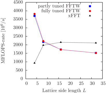 |
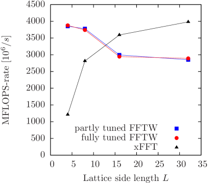 |
| (a) | (b) |
For clarification it is explicitly pointed out that the xFFT implementation is not based on a superior algorithm in the sense that it would require a lower number of floating point operations. In fact, rather the opposite is the case, since the algorithmic foundation of the latter implementation is the multi-dimensional Cooley-Tukey approach which is clearly not the most efficient algorithm in terms of floating point operations as discussed above. The improved performance is thus completely due to a more efficient software realization of the underlying algorithm.
To elaborate more on that the reader is assumed to be familiar with the basic concepts of the hardware architecture underlying modern computer systems555A general introduction to modern computer hardware architecture can be found in LABEL:Hennessy:2006zu. An introduction to corresponding software optimization strategies for the particular case of AMD systems can be found in LABEL:AMDOpti:2009zu.. As a first step towards an understanding of how this improved efficiency level can be achieved, we will estimate the performance of the competing implementations FFTW and xFFT in terms of the ratio between the observed MFLOPS-rate as specified in Eq. (B.12) and the theoretically possible rate , which is denoted as peak performance. The considered AMD processor core possesses a separate addition and a separate multiplication SSE-unit that can independently of each other perform two double precision operations simultaneously which, however, asymptotically takes 2 CPU-cycles in pipelining mode to complete. In the considered setup the total number of double precision floating point operations that can theoretically be performed in each second thus sums up to . If one compares this number with the MFLOPS-rates presented in Fig. B.2a for the largest presented volume, one finds that the performance of the FFTW implementation is around while the one of the xFFT code is around .
From this comparison one can infer that it is not so much the number of floating point operations that limit the speed of the considered FFT implementations but rather other, administrative processes, such as the transportation of data from the main memory to the processor and vice versa. To minimize the required data traffic the xFFT implementation is explicitly based on two-dimensional Fourier transforms that are, for instance, first performed along the dimensions (0,1) and then along the dimensions (2,3). This approach then guarantees that the overall data amount of the transformed vector , being in total bytes, is only transported twice from main memory to the processor and back for one four-dimensional FFT, provided that the data of each individual two-dimensional Fourier transform, which will be referred to as a two-dimensional data slice in the following, can simultaneously be stored in the data cache. Contrary to that one would need four such data transfers, if one would first perform all one-dimensional transforms along the first space-time dimension, then all one-dimensional transforms along the second dimension and so on. This observation is well-known in the literature. The crucial question is, whether the aforementioned data slices can indeed simultaneously be stored in the data cache.
To address the latter issue, let us now consider the specific example of the volume. In that scenario the latter data slices have the size bytes, i.e. here. From the perspective of the total data amount, these data slices should perfectly fit at least into the Level 2 cache. There is, however, a crucial obstacle that can actually block the effective caching of the considered data slices. This problem arises from the method how the cache cell address that is supposed to hold a particular datum, read from the main memory address , is determined. In practice this is, at least in part, done by a modulo operation according to
| (B.13) |
where is the size of the cache, i.e. usually a power of two. This is called an associative cache mapping strategy in the literature. The problem now arises, for instance, when a one-dimensional Fourier transform is performed along the outer most index666To map the multi-dimensional vector index of into the main memory, a single sequential address has to be computed. This is done here according to . In that sense would be the outer most index here. of the vector . In that case the memory addresses involved in that particular transformation would all differ by multiples of . In the here considered case one would typically have , while is also a power of two like , which finally results in all data involved in the aforementioned Fourier transform to be mapped to the same cache address, thus kicking each other out of the cache. The result is a so-called low cache coherency which leads to the necessity of reloading the same data multiple times from the main memory.
This problem is manifestly circumvent in the xFFT implementation by using internal buffer structures that explicitly break the latter translation invariance of the cache addresses associated to the buffer addresses storing the aforementioned two-dimensional data slices. It is remarked that these cache coherency considerations have a severe impact on the overall performance.
Another crucial point is the efficient prefetching of the required data as well as the associated question of data locality. The notion of ’prefetching’ refers here to the possibility that the processor can notify the memory controller that a certain memory address will be requested in the future, thus allowing the memory controller to begin already with the data loading process, while the processor can simultaneously continue with some other operations. In an optimal scenario this can prevent the processor from having to wait for data that have not yet been delivered to the processor. An efficient prefetching strategy is thus vital for the success of many software implementations. Due to the above described bit-reversed reordering of the transformed vector this is especially true, and unfortunately also more complicated, in the case of a FFT implementation.
In such a prefetching strategy it is very beneficial to request the data in sequential order, which is known as the problem of data locality. The rationale is that the memory latency times for delivering the datum at a certain memory address depend significantly on the previously requested memory address. This is because the main memory is built in form of a matrix consisting of rows and columns, where each matrix cell can store information. When a certain memory address is requested, the matrix row containing that address has to be activated, unless it has already been activated in the previous memory access. This row activation takes some time which is known as the row address strobe (RAS-latency). In a subsequent step the column of the matrix containing the requested memory address has to be activated, which again takes some additional time known as column address strobe (CAS-latency). If one addresses memory in some incoherent order, such as in a bit-reversed order for instance, one is confronted with the penalty of having to wait for the RAS- and CAS-latency times in each memory access. If one, on the other hand, accesses the same data in a coherent order, one profits from the memory matrix row staying activated as long as possible, thus reducing the amount of RAS-latency penalties encountered.
In the implemented xFFT code special effort has been invested to improve the order in which the data is requested from the main memory to optimize data locality. In total the above described techniques sum up to the performance advantage on the considered AMD architecture already presented in Fig. B.2a. It is further remarked that the xFFT implementation, which has originally been designed for the latter architecture, is less advantageous on Intel machines. On an Intel Core 2 CPU it was, however, still found to be faster than the FFTW implementation in the here considered scenario by around .
Finally, some remarks shall be given concerning the parallelization of the Fourier transform. It is well known that the computation of the underlying lower dimensional Fourier transforms can efficiently be assigned to different, remote computer nodes, see e.g. LABEL:FFTWHomepage. With this approach the Fourier transform can be split up into a large number of smaller tasks running on remote nodes, which finally leads to a significantly smaller wall clock runtime. The efficiency of this approach in terms of achieved versus theoretical operation counts, however, suffers from the additional requirement of network communication and is thus usually smaller than that of a single node computation. In the context of the here considered Higgs-Yukawa model it was therefore found to be more suitable, at least for the studied lattice sizes, to use a shared memory parallelization on a single computer mode. Though the scalability of such an approach is restricted by the number of available CPU cores on that single node, the advantage of this method lies in the higher achieved efficiency, thus ultimately allowing to generate more field configurations in total with a given amount of numerical resources than it would have been possible with a remote node parallelization ansatz. The applicability of the shared memory approach, of course, depends on the question, whether a single node provides enough performance to process a single lattice calculation, which, however, is the case thanks to the algorithmic improvements in chapter 5.
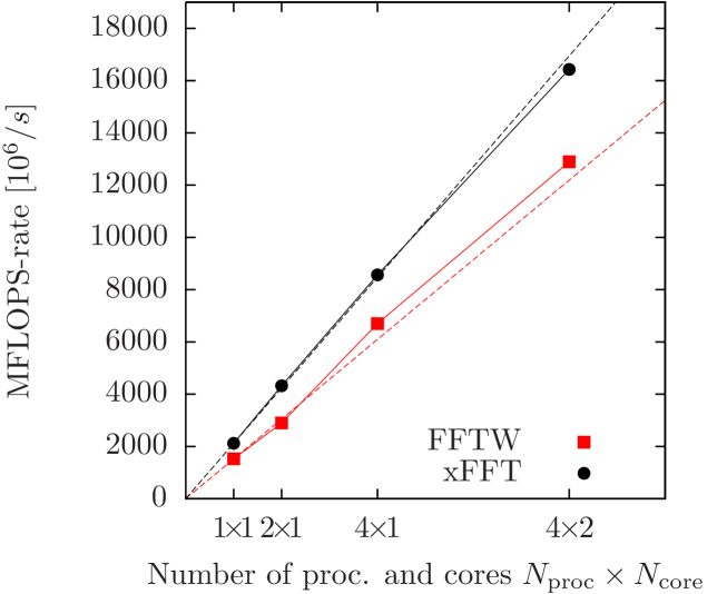
An example of the MFLOPS-rates observed for the FFT computation when employing two CPU cores on a single node is presented in Fig. B.2b. In both cases, i.e. for the FFTW as well as the xFFT implementation, one observes a good scaling behaviour in comparison with Fig. B.2a at least on the largest presented lattice volume. If one naively employs an increasing number of CPU cores for the FFT computation on a single node, however, the achieved MFLOPS-rates will finally run into a plateau. This is because the memory bus bandwidth will eventually become the limiting factor.
A decent way to overcome this limitation is to exploit the Non-Uniform Memory Architecture (NUMA) [217] underlying the AMD systems installed in the aforementioned HP XC4000 System. In this setup each computer node possesses processors each consisting of two CPU-cores. Attached to each processor is a separate memory bus connecting the respective processor to its individually associated main memory. The result is that each processor can access its own main memory independently from the work load of the other processors and their respective memory buses. Moreover, the processors are also connected to each other by some additional bus, denoted as Hyper-Transport bus, which is dedicated to the inter-processor communication.
The idea here is to split up the pseudo fermion vector according to its inner index into pieces and to distribute these pieces to the different main memories. This allows then each of the processors to perform the Fourier transform on its respective sub vector without interfering with the computations on the other processors. On each processor the respective work load can then efficiently be shared among the two available cores as demonstrated in Fig. B.2b. The scaling of the total MFLOPS-rate resulting from this approach is presented in Fig. B.3 for the case of a node with having CPU cores each and very good scaling behaviour is observed in both cases, i.e. for the FFTW as well as the xFFT implementation, while again the xFFT approach yields significantly better performance.
It is further remarked that this distributed storage of the vector is maintained during the whole lattice computation, since most other operations on the vector , such as vector additions, scalar products and even the application of the operator can easily be split up into corresponding non-interfering tasks, provided that the inner index is adequately distributed. In such a scenario it is only the application of the momentum space representation of the Dirac operator being non-diagonal only with respect to the inner index that then finally mixes vector components assigned to different processor memories. In this approach the application of the operator is thus the only operation that does not scale with the number . It can, however, still be efficiently implemented thanks to the fast Hyper-Transport buses connecting the processors with each other.
As a concluding remark it is summarized that high-performance implementations of Fast Fourier Transforms in four dimensions are indeed available, which thus allows for the efficient construction of the overlap Dirac operator as described in section 3.5. Though not explicitly discussed here and not implemented within the xFFT approach, this includes also the situation of lattice side lengths being non-powers of two decomposable, however, into small prime factors as discussed, for instance, in LABEL:FFTW05.
Acknowledgments
Over the last years I received a lot of warm and inspiring support from many individuals and organizations, my supervisors, colleagues, friends, relatives and other supporters, I feel deeply indebted to. Here, I would like to take the opportunity to express my gratitude to these persons and to name them individually.
First of all, I would like to cordially thank my direct supervisor Dr. habil. Karl Jansen for guiding and mentoring this work in a very close, friendly, inspiring, and supportive manner, for sharing his ideas and great experience on Higgs-Yukawa models in particular and lattice theory in general, and especially for the endless hours he spent with me on discussing the open questions of this research project. His experience was extremely helpful for identifying promising investigation strategies and safely avoiding conceptual impasses. Moreover, I am thankful for him providing me the opportunity to participate in a series of international conferences and schools, which greatly promoted the success of this work.
Of equal importance has been the continuous and ongoing support of my supervising professor Prof. Dr. Michael Müller-Preussker that has always been constituting the robust and reliable fundament, which is required for the successful completion of a PhD project. It has been his scientific advice and shared experience, from which I could tremendously profit over the last years. Moreover, the friendly and warm atmosphere in his working group has driven the time spent on the project into a very pleasant experience. Especially, I would like to thank him for his personal engagement that allowed me to benefit from a PhD scholarship provided by the Deutsche Telekom Stiftung and to participate in the annual Nobel laureate meeting in Lindau 2008. For all that I feel indebted to him.
Moreover, I would like to express my gratitude to the Deutsche Telekom Stiftung for supporting me by providing a PhD scholarship and for granting additional funding for traveling and attending conferences. The generous financial aid coming along with that scholarship enabled me in particular to spend a considerable fraction of my PhD research project abroad. I am therefore very thankful to the numerous people enabling the work of this organization. In particular, I would like to express my special gratitude to Prof. Dr. Dr. h.c. Manfred Erhardt for continuously supporting and mentoring me over the last couple of years in a personal manner and from a non-physical perspective.
During my half-year stay in the research group of Prof. Julius Kuti at the University of California, San Diego, I received a lot of warm and friendly support from the local group members and collaborators, among them Prof. Kieran Holland, Dr. Daniel Nogradi, Chris Schroeder, Pamela Smilo, and in particular from Prof. Julius Kuti, who originally invited me to San Diego, and from whom I could learn a lot about Fourier acceleration techniques and many other details of Higgs-Yukawa systems. I am very thankful for the helpful and inspiring discussions and moreover for the great hospitality that I experienced during that stay.
Special thanks go to Jim Kallarackal, who helped me a lot in broadening my understanding of and knowledge on general quantum field theory through uncountable discussions, for conversations and collaborations on specific issues of the considered Higgs-Yukawa model, for instance contributing certain routines of the software code analyzing the generated field configurations, and for his helpful comments on this manuscript.
Also, I would like to thank Prof. Jaume Carbonell, Dr. Jean-Christian Anglès d’Auriac, and Dr. Feliciano de Soto for inviting me to the University of Grenoble, France, for a research visit. In particular, I am grateful for discussions about the details of alternative physical applications of the studied Higgs-Yukawa model in the framework of nuclear theory as well as for their great hospitality.
Moreover, I thank Prof. Dr. Andreas Wipf, Prof. Dr. Holger Gies, Dr. Tobias Kästner, and Christian Wozar for inspiring discussions about related scalar-fermion systems and for their hospitality.
I am also grateful to Dr. Dru Renner, Dr. Georg von Hippel, and Dr. Rainer Sommer for many helpful hints and comments on general lattice techniques and quantum field theory.
During my daily work time I always felt surrounded by friendly and cooperative colleagues. In particular, I would like to name my current and former office workmates Xu Feng, Jenifer Gonzalez Lopez, Isaac Hailperin, Petra Kovacikova, Marina Marinkovic, and Andreas Nube, who made working here a very pleasant experience. I would like to thank all of them for many motivating and instructive conversations – and moreover – simply for the great time over the last years.
Additional funding for my PhD position before and after the above scholarship and for attending conferences has been provided by the DFG through the DFG-project Mu932/4-1, the Humboldt-University Berlin, the Wilhelm und Else Heraeus-Stiftung, as well as DESY in Zeuthen, which I am very grateful for.
The major fraction of the computational workload has been performed on the HP XC4000 System at the Scientific Supercomputing Center of the University Karlsruhe, Germany. The work of the local staff maintaining and running that machine has always been characterized by a high degree of reliability and professionalism which, together with the generous allocation of computing resources, greatly promoted the success of this study. I also would like to acknowledge the support of the SGI system HLRN-II at the HLRN Supercomputing Service Berlin-Hannover, Germany.
Last but not least I would like to thank my family, in particular my parents Brigitte and Dankward Gerhold as well as my sister Rosemarie Gerhold, and my girlfriend Cornelia Kipping, who have always been there for me. Without their great moral support this work would not have been possible. Thank you!
References
- Gell-Mann [1964] M. Gell-Mann. A Schematic Model of Baryons and Mesons. Phys. Lett., 8:214–215, 1964. doi: 10.1016/S0031-9163(64)92001-3.
- Zweig [1964] G. Zweig. An SU(3) model for strong interaction symmetry and its breaking. CERN-TH-401/8419, 1964.
- Peskin and Schroeder [2008] M. E. Peskin and D. V. Schroeder. An Introduction to Quantum Field Theory (Frontiers in Physics). Perseus Books, 2008.
- Einstein [1916] A. Einstein. The foundation of the general theory of relativity. Annalen Phys., 49:769–822, 1916. doi: 10.1002/andp.200590044.
- Becker et al. [2006] K. Becker, M. Becker, and J. E. Schwarz. String Theory and M-Theory: A Modern Introduction. Cambridge University Press, 2006.
- Thiemann [2008] T. Thiemann. Modern Canonical Quantum General Relativity. Cambridge University Press, 2008.
- Cheng and Li [1988] T. P. Cheng and L. F. Li. Gauge Theory of elementary particle physics. Oxford University Press, 1988.
- Feynman [1998] R. P. Feynman. Quantum Electrodynamics. Perseus Books, 1998.
- Aoyama et al. [2008] T. Aoyama, M. Hayakawa, T. Kinoshita, and M. Nio. Revised value of the eighth-order QED contribution to the anomalous magnetic moment of the electron. Phys. Rev., D77:053012, 2008. doi: 10.1103/PhysRevD.77.053012.
- Amsler et al. [2008] C. Amsler et al. Review of particle physics. Phys. Lett., B667:1, 2008. doi: 10.1016/j.physletb.2008.07.018.
- Greiner et al. [2007] W. Greiner, S. Schramm, and E. Stein. Quantum Chromodynamics. Springer, 2007.
- Han and Nambu [1965] M. Y. Han and Yoichiro Nambu. Three-triplet model with double SU(3) symmetry. Phys. Rev., 139:B1006–B1010, 1965. doi: 10.1103/PhysRev.139.B1006.
- Politzer [1973] H. D. Politzer. Reliable perturbative results for strong interactions? Phys. Rev. Lett., 30:1346–1349, 1973. doi: 10.1103/PhysRevLett.30.1346.
- Gross and Wilczek [1973] D. J. Gross and F. Wilczek. Ultraviolet behavior of non-Abelian gauge theories. Phys. Rev. Lett., 30:1343–1346, 1973. doi: 10.1103/PhysRevLett.30.1343.
- Bjorken [1969] J. D. Bjorken. Asymptotic Sum Rules at Infinite Momentum. Phys. Rev., 179:1547–1553, 1969. doi: 10.1103/PhysRev.179.1547.
- Miller et al. [1972] G. Miller et al. Inelastic electron-Proton Scattering at Large Momentum Transfers. Phys. Rev., D5:528, 1972. doi: 10.1103/PhysRevD.5.528.
- Wilson [1974] K. G. Wilson. Confinement of quarks. Phys. Rev., D10:2445–2459, 1974. doi: 10.1103/PhysRevD.10.2445.
- Greensite [ed.] J. P. Greensite (ed.) and S. Olejník (ed.). Confinement, Topology, and Other Non-Pertubative Aspects of QCD. Springer, 2002.
- Sudarshan and Marshak [1958] E. C. G. Sudarshan and R. E. Marshak. Chirality Invariance and the Universal Fermi Interaction. Phys. Rev., 109(5):1860–1862, Mar 1958. doi: 10.1103/PhysRev.109.1860.2.
- Feynman and Gell-Mann [1958] R. P. Feynman and M. Gell-Mann. Theory of the Fermi Interaction. Phys. Rev., 109(1):193–198, Jan 1958. doi: 10.1103/PhysRev.109.193.
- Glashow [1961] S. L. Glashow. Partial Symmetries of Weak Interactions. Nucl. Phys., 22:579–588, 1961. doi: 10.1016/0029-5582(61)90469-2.
- Salam [1968] A. Salam. Weak and electromagnetic interactions. Elementary Particle Physics: Relativistic Groups and Analyticity, Nobel Symposium No 8 (Ed. N. Svartholm, Almqvist and Wiksell, Stockholm), 1968.
- Weinberg [1967] S. Weinberg. A Model of Leptons. Phys. Rev. Lett., 19:1264–1266, 1967. doi: 10.1103/PhysRevLett.19.1264.
- ’t Hooft [1971a] G. ’t Hooft. Renormalization of Massless Yang-Mills Fields. Nucl. Phys., B33:173–199, 1971a. doi: 10.1016/0550-3213(71)90395-6.
- ’t Hooft [1971b] G. ’t Hooft. Renormalizable Lagrangians for massive Yang-Mills fields. Nucl. Phys., B35:167–188, 1971b. doi: 10.1016/0550-3213(71)90139-8.
- ’t Hooft and Veltman [1972] G. ’t Hooft and M. J. G. Veltman. Regularization and Renormalization of Gauge Fields. Nucl. Phys., B44:189–213, 1972. doi: 10.1016/0550-3213(72)90279-9.
- Rosner [2001] J. L. Rosner. The Standard model in 2001. arXiv, hep-ph/0108195, 2001. Lectures given at 55th Scottish Universities Summer School in Physics: Heavy Flavor Physics, St. Andrews, Scotland, 7-23 Aug 2001.
- Altarelli and Grunewald [2004] G. Altarelli and M. W. Grunewald. Precision electroweak tests of the standard model. Phys. Rept., 403-404:189–201, 2004. doi: 10.1016/j.physrep.2004.08.013.
- Arnison et al. [1983a] G. Arnison et al. Experimental observation of isolated large transverse energy electrons with associated missing energy at s**(1/2) = 540-GeV. Phys. Lett., B122:103–116, 1983a.
- Banner et al. [1983] M. Banner et al. Observation of single isolated electrons of high transverse momentum in events with missing transverse energy at the CERN anti-p p collider. Phys. Lett., B122:476–485, 1983. doi: 10.1016/0370-2693(83)91605-2.
- Arnison et al. [1983b] G. Arnison et al. Experimental observation of lepton pairs of invariant mass around 95-GeV/c**2 at the CERN SPS collider. Phys. Lett., B126:398–410, 1983b. doi: 10.1016/0370-2693(83)90188-0.
- Higgs [1964] P. W. Higgs. Broken symmetries and the masses of gauge bosons. Phys. Rev. Lett., 13(16):508–509, Oct 1964. doi: 10.1103/PhysRevLett.13.508.
- Englert and Brout [1964] F. Englert and R. Brout. Broken symmetry and the mass of gauge vector mesons. Phys. Rev. Lett., 13(9):321–323, Aug 1964. doi: 10.1103/PhysRevLett.13.321.
- Guralnik et al. [1964] G. S. Guralnik, C. R. Hagen, and T. W. B. Kibble. Global conservation laws and massless particles. Phys. Rev. Lett., 13(20):585–587, Nov 1964. doi: 10.1103/PhysRevLett.13.585.
- Nambu and Jona-Lasinio [1961a] Y. Nambu and G. Jona-Lasinio. Dynamical Model of Elementary Particles Based on an Analogy with Superconductivity. I. Phys. Rev., 122(1):345–358, Apr 1961a. doi: 10.1103/PhysRev.122.345.
- Nambu and Jona-Lasinio [1961b] Y. Nambu and G. Jona-Lasinio. Dynamical Model of Elementary Particles Based on an Analogy with Superconductivity. II. Phys. Rev., 124(1):246–254, Oct 1961b. doi: 10.1103/PhysRev.124.246.
- Goldstone [1961] J. Goldstone. Field Theories with Superconductor Solutions. Nuovo Cim., 19:154–164, 1961. doi: 10.1007/BF02812722.
- Yukawa [1935] H. Yukawa. On the interaction of elementary particles. Proc. Phys. Math. Soc. Jap., 17:48–57, 1935.
- Goldstone et al. [1962] J. Goldstone, A. Salam, and S. Weinberg. Broken Symmetries. Phys. Rev., 127:965–970, 1962. doi: 10.1103/PhysRev.127.965.
- Evans [ed.] L. Evans (ed.) and P. Bryant (ed.). LHC Machine. Journal of Instrumentation, 3(08):S08001, 2008. URL http://stacks.iop.org/1748-0221/3/S08001.
- The LEP Electroweak Working Group [2009] The LEP Electroweak Working Group. LEP Electroweak Working Group homepage. http://lepewwg.web.cern.ch/LEPEWWG, 2009.
- Aizenman [1981] M. Aizenman. Proof of the Triviality of phi**4 in D-Dimensions Field Theory and Some Mean Field Features of Ising Models for D. Phys. Rev. Lett., 47:1–4, 1981. doi: 10.1103/PhysRevLett.47.1.
- Fröhlich [1982] J. Fröhlich. On the Triviality of Lambda (phi**4) in D-Dimensions Theories and the Approach to the Critical Point in D Four-Dimensions. Nucl. Phys., B200:281–296, 1982. doi: 10.1016/0550-3213(82)90088-8.
- Lüscher and Weisz [1989] M. Lüscher and P. Weisz. Scaling Laws and Triviality Bounds in the Lattice phi**4 Theory. 3. N Component Model. Nucl. Phys., B318:705, 1989. doi: 10.1016/0550-3213(89)90637-8.
- Hasenfratz et al. [1987] A. Hasenfratz, K. Jansen, C. B. Lang, T. Neuhaus, and H. Yoneyama. The Triviality Bound of the Four Component phi**4 Model. Phys. Lett., B199:531, 1987. doi: 10.1016/0370-2693(87)91622-4.
- Kuti et al. [1988] J. Kuti, L. Lin, and Y. Shen. Upper Bound on the Higgs Mass in the Standard Model. Phys. Rev. Lett., 61:678, 1988. doi: 10.1103/PhysRevLett.61.678.
- Hasenfratz et al. [1989] A. Hasenfratz et al. Study of the Four Component phi**4 Model. Nucl. Phys., B317:81, 1989. doi: 10.1016/0550-3213(89)90562-2.
- Göckeler et al. [1993] M. Göckeler, H. A. Kastrup, T. Neuhaus, and F. Zimmermann. Scaling analysis of the 0(4) symmetric Phi**4 theory in the broken phase. Nucl. Phys., B404:517–555, 1993. doi: 10.1016/0550-3213(93)90489-C.
- Kamionkowski [2007] M. Kamionkowski. Dark Matter and Dark Energy. arXiv, 0706.2986 [astro-ph], 2007.
- Akhmedov [1999] E. K. Akhmedov. Neutrino physics. arXiv, hep-ph/0001264, 1999. Lectures given at ICTP Summer School in Particle Physics, Trieste, Italy, 7 Jun - 9 Jul 1999.
- Cline [2006] J. M. Cline. Baryogenesis. arXiv, hep-ph/0609145, 2006. Lectures given at Les Houches Summer School - Session 86: Particle Physics and Cosmology: The Fabric of Spacetime, Les Houches, France, 31 Jul - 25 Aug 2006.
- Quigg [2009] C. Quigg. Unanswered Questions in the Electroweak Theory. arXiv, 0905.3187 [hep-ph], 2009.
- Nilles [1984] H. P. Nilles. Supersymmetry, supergravity and particle physics. Physics Reports, 110(1-2):1 – 162, 1984. ISSN 0370-1573. doi: DOI:10.1016/0370-1573(84)90008-5.
- Georgi and Glashow [1974] H. Georgi and S. L. Glashow. Unity of All Elementary Particle Forces. Phys. Rev. Lett., 32:438–441, 1974. doi: 10.1103/PhysRevLett.32.438.
- Schmaltz and Tucker-Smith [2005] M. Schmaltz and D. Tucker-Smith. Little Higgs Review. Ann. Rev. Nucl. Part. Sci., 55:229–270, 2005. doi: 10.1146/annurev.nucl.55.090704.151502.
- Perez-Lorenzana [2005] A. Perez-Lorenzana. An introduction to extra dimensions. J. Phys. Conf. Ser., 18:224–269, 2005. doi: 10.1088/1742-6596/18/1/006.
- Cabibbo et al. [1979] N. Cabibbo, L. Maiani, G. Parisi, and R. Petronzio. Bounds on the Fermions and Higgs Boson Masses in Grand Unified Theories. Nucl. Phys., B158:295, 1979. doi: 10.1016/0550-3213(79)90167-6.
- Linde [1976] A. D. Linde. Dynamical Symmetry Restoration and Constraints on Masses and Coupling Constants in Gauge Theories. JETP Lett., 23:64–67, 1976.
- Weinberg [1976] S. Weinberg. Mass of the Higgs Boson. Phys. Rev. Lett., 36:294–296, 1976. doi: 10.1103/PhysRevLett.36.294.
- Linde [1977] A. D. Linde. On the Vacuum Instability and the Higgs Meson Mass. Phys. Lett., B70:306, 1977. doi: 10.1016/0370-2693(77)90664-5.
- Sher [1989] M. Sher. Electroweak Higgs Potentials and Vacuum Stability. Phys. Rept., 179:273–418, 1989. doi: 10.1016/0370-1573(89)90061-6.
- Lindner et al. [1989] M. Lindner, M. Sher, and H. W. Zaglauer. Probing Vacuum Stability Bounds at the Fermilab Collider. Phys. Lett., B228:139, 1989. doi: 10.1016/0370-2693(89)90540-6.
- Altarelli and Isidori [1994] G. Altarelli and G. Isidori. Lower limit on the Higgs mass in the standard model: An Update. Phys. Lett., B337:141–144, 1994. doi: 10.1016/0370-2693(94)91458-3.
- Casas et al. [1995] J. A. Casas, J. R. Espinosa, and M. Quiros. Improved Higgs mass stability bound in the standard model and implications for supersymmetry. Phys. Lett., B342:171–179, 1995. doi: 10.1016/0370-2693(94)01404-Z.
- Casas et al. [1996] J. A. Casas, J. R. Espinosa, and M. Quiros. Standard Model stability bounds for new physics within LHC reach. Phys. Lett., B382:374–382, 1996. doi: 10.1016/0370-2693(96)00682-X.
- Dashen and Neuberger [1983] R. F. Dashen and H. Neuberger. How to Get an Upper Bound on the Higgs Mass. Phys. Rev. Lett., 50:1897, 1983. doi: 10.1103/PhysRevLett.50.1897.
- Lindner [1986] M. Lindner. Implications of Triviality for the Standard Model. Zeit. Phys., C31:295, 1986. doi: 10.1007/BF01479540.
- Dicus and Mathur [1973] D. A. Dicus and V. S. Mathur. Upper bounds on the values of masses in unified gauge theories. Phys. Rev., D7:3111–3114, 1973. doi: 10.1103/PhysRevD.7.3111.
- Lee et al. [1977] B. W. Lee, C. Quigg, and H. B. Thacker. Weak Interactions at Very High-Energies: The Role of the Higgs Boson Mass. Phys. Rev., D16:1519, 1977. doi: 10.1103/PhysRevD.16.1519.
- Marciano et al. [1989] W. J. Marciano, G. Valencia, and S. Willenbrock. Renormalization group improved unitarity bounds on the Higgs boson and top quark masses. Phys. Rev., D40:1725, 1989. doi: 10.1103/PhysRevD.40.1725.
- Hagiwara et al. [2002] K. Hagiwara et al. Review of particle physics. Phys. Rev., D66:010001, 2002. doi: 10.1103/PhysRevD.66.010001.
- O’Raifeartaigh et al. [1986] L. O’Raifeartaigh, A. Wipf, and H. Yoneyama. The constraint effective potential. Nucl. Phys., B271:653, 1986. doi: 10.1016/S0550-3213(86)80031-1.
- Holland and Kuti [2004] K. Holland and J. Kuti. How light can the Higgs be. Nucl. Phys. Proc. Suppl., 129:765–767, 2004.
- Holland [2005] K. Holland. Triviality and the Higgs mass lower bound. Nucl. Phys. Proc. Suppl., 140:155–161, 2005.
- Lin et al. [1991] L. Lin, I. Montvay, H. Wittig, and G. Münster. A U(1)-L x U(1)-R symmetric Yukawa model in the phase with spontaneously broken symmetry. Nucl. Phys., B355:511–548, 1991. doi: 10.1016/0550-3213(91)90124-G.
- Rothe [2005] H. J. Rothe. Lattice gauge theories. World Scientific Lecture Notes in Physics, 3rd revised edition edition, 2005.
- Shamir [1996] Y. Shamir. Lattice Chiral Fermions. Nucl. Phys. Proc. Suppl., 47:212–227, 1996. doi: 10.1016/0920-5632(96)00046-1.
- Lüscher [1998] M. Lüscher. Exact chiral symmetry on the lattice and the Ginsparg- Wilson relation. Phys. Lett., B428:342–345, 1998.
- Ginsparg and Wilson [1982] P. H. Ginsparg and K. G. Wilson. A remnant of chiral symmetry on the lattice. Phys. Rev., D25:2649, 1982.
- Niedermayer [1999] F. Niedermayer. Exact chiral symmetry, topological charge and related topics. Nucl. Phys. Proc. Suppl., 73:105–119, 1999. doi: 10.1016/S0920-5632(99)85011-7.
- Lüscher [1999] M. Lüscher. Abelian chiral gauge theories on the lattice with exact gauge invariance. Nucl. Phys., B549:295–334, 1999. doi: 10.1016/S0550-3213(99)00115-7.
- Lüscher [2000] M. Lüscher. Chiral gauge theories revisited. arXiv, hep-th/0102028, 2000. Lectures given at International School of Subnuclear Physics: 38th Course: Theory and Experiment Heading for New Physics, Erice, Italy, 27 Aug - 5 Sep 2000.
- Kadoh and Kikukawa [2008a] D. Kadoh and Y. Kikukawa. A construction of the Glashow-Weinberg-Salam model on the lattice with exact gauge invariance. JHEP, 05:095, 2008a. doi: 10.1088/1126-6708/2008/05/095.
- Kadoh et al. [2004] D. Kadoh, Y. Kikukawa, and Y. Nakayama. Solving the local cohomology problem in U(1) chiral gauge theories within a finite lattice. JHEP, 12:006, 2004. doi: 10.1088/1126-6708/2004/12/006.
- Kadoh and Kikukawa [2008b] D. Kadoh and Y. Kikukawa. A simple construction of fermion measure term in U(1) chiral lattice gauge theories with exact gauge invariance. JHEP, 02:063, 2008b. doi: 10.1088/1126-6708/2008/02/063.
- Bhanot et al. [1991] G. Bhanot, K. Bitar, U. M. Heller, and H. Neuberger. Phi**4 on F(4): Numerical results. Nucl. Phys., B353:551–564, 1991. doi: 10.1016/0550-3213(91)90348-2.
- Lin et al. [1993] L. Lin, I. Montvay, G. Münster, M. Plagge, and H. Wittig. Bounds on the renormalized couplings in an SU(2)-L x SU(2)-R symmetric Yukawa model. Phys. Lett., B317:143–150, 1993. doi: 10.1016/0370-2693(93)91584-A.
- Bock et al. [1993] W. Bock, C. Frick, J. Smit, and J. C. Vink. Can the couplings in the fermion Higgs sector of the Standard Model be strong? Nucl. Phys., B400:309–346, 1993. doi: 10.1016/0550-3213(93)90408-H.
- Lee et al. [1990] I.-H. Lee, J. Shigemitsu, and R. E. Shrock. Lattice study of a Yukawa theory with a real scalar field. Nucl. Phys., B330:225, 1990. doi: 10.1016/0550-3213(90)90309-2.
- Montvay [1985] I. Montvay. Correlations in the SU(2) fundamental Higgs model. Phys. Lett., B150:441, 1985. doi: 10.1016/0370-2693(85)90462-9.
- Evertz et al. [1986] H. G. Evertz, J. Jersak, C. B. Lang, and T. Neuhaus. SU(2) Higgs boson and vector boson masses on the lattice. Phys. Lett., B171:271, 1986. doi: 10.1016/0370-2693(86)91547-9.
- Hasenfratz and Neuhaus [1988] A. Hasenfratz and T. Neuhaus. Upper bound estimate for the Higgs mass from the lattice regularized Weinberg-Salam model. Nucl. Phys., B297:205, 1988. doi: 10.1016/0550-3213(88)90206-4.
- Evertz et al. [1989] H. G. Evertz, E. Katznelson, P. Lauwers, and M. Marcu. Towards a better quantitative understanding of the SU(2) Higgs model. Phys. Lett., B221:143, 1989. doi: 10.1016/0370-2693(89)91488-3.
- Smit [1990] J. Smit. Standard model and chiral gauge theories on the lattice. Nucl. Phys. Proc. Suppl., 17:3–16, 1990.
- Shigemitsu [1991] J. Shigemitsu. Higgs-Yukawa chiral models. Nucl. Phys. Proc. Suppl., 20:515–527, 1991.
- Golterman [1991] M. F. L. Golterman. Lattice chiral gauge theories: Results and problems. Nucl. Phys. Proc. Suppl., 20:528–541, 1991.
- De and Jersák [1991] A. K. De and J. Jersák. Yukawa models on the lattice. HLRZ Jülich, HLRZ 91-83, preprint edition, 1991.
- Montvay and Münster [1997] I. Montvay and G. Münster. Quantum Fields on a Lattice (Cambridge Monographs on Mathematical Physics). Cambridge University Press, 1997.
- Golterman et al. [1992] M. F. L. Golterman, D. N. Petcher, and E. Rivas. On the Eichten-Preskill proposal for lattice chiral gauge theories. Nucl. Phys. Proc. Suppl., 29BC:193–199, 1992.
- Jansen [1996] K. Jansen. Domain wall fermions and chiral gauge theories. Phys. Rept., 273:1–54, 1996.
- Bhattacharya et al. [2006] T. Bhattacharya, M. R. Martin, and E. Poppitz. Chiral lattice gauge theories from warped domain walls and Ginsparg-Wilson fermions. Phys. Rev., D74:085028, 2006.
- Gerhold and Jansen [2007a] P. Gerhold and K. Jansen. The phase structure of a chirally invariant lattice Higgs-Yukawa model for small and for large values of the Yukawa coupling constant. JHEP, 09:041, 2007a.
- Giedt and Poppitz [2007] J. Giedt and E. Poppitz. Chiral Lattice Gauge Theories and The Strong Coupling Dynamics of a Yukawa-Higgs Model with Ginsparg-Wilson Fermions. JHEP, 10:076, 2007. doi: 10.1088/1126-6708/2007/10/076.
- Gerhold and Jansen [2007b] P. Gerhold and K. Jansen. The phase structure of a chirally invariant lattice Higgs-Yukawa model - numerical simulations. JHEP, 10:001, 2007b. doi: 10.1088/1126-6708/2007/10/001.
- Poppitz and Shang [2007] E. Poppitz and Y. Shang. Lattice chirality and the decoupling of mirror fermions. arXiv:, 0706.1043 [hep-th], 2007.
- Fodor et al. [2007] Z. Fodor, K. Holland, J. Kuti, D. Nogradi, and C. Schroeder. New Higgs physics from the lattice. PoS, LAT2007:056, 2007.
- Gerhold and Jansen [2009] P. Gerhold and K. Jansen. Lower Higgs boson mass bounds from a chirally invariant lattice Higgs-Yukawa model with overlap fermions. JHEP, 07:025, 2009.
- Frezzotti and Jansen [1997] R. Frezzotti and K. Jansen. A polynomial hybrid Monte Carlo algorithm. Phys. Lett., B402:328–334, 1997. doi: 10.1016/S0370-2693(97)00475-9.
- Lüscher [1991a] M. Lüscher. Two particle states on a torus and their relation to the scattering matrix. Nucl. Phys., B354:531–578, 1991a. doi: 10.1016/0550-3213(91)90366-6.
- Lüscher [1991b] M. Lüscher. Signatures of unstable particles in finite volume. Nucl. Phys., B364:237–254, 1991b. doi: 10.1016/0550-3213(91)90584-K.
- Feynman [1948] R. P. Feynman. Space-time approach to nonrelativistic quantum mechanics. Rev. Mod. Phys., 20:367–387, 1948. doi: 10.1103/RevModPhys.20.367.
- Feynman [1950] R. P. Feynman. Mathematical formulation of the quantum theory of electromagnetic interaction. Phys. Rev., 80:440–457, 1950. doi: 10.1103/PhysRev.80.440.
- Matthews and Salam [1955] P. T. Matthews and A. Salam. Propagators of quantized field. Nuovo Cim., 2:120–134, 1955. doi: 10.1007/BF02856011.
- Berezin [1966] F. A. Berezin. The method of second quantization. Academic Press, 1966.
- Candlin [1956] D. J. Candlin. On Sums over Trajectories for Systems with Fermi Statistics. Nuovo Cim., 4:231, 1956.
- Wick [1954] G. C. Wick. Properties of Bethe-Salpeter Wave Functions. Phys. Rev., 96:1124–1134, 1954. doi: 10.1103/PhysRev.96.1124.
- Schwinger [1958] J. Schwinger. On the Euclidean structure of relativistic field theory. Proc. Natl. Acad. Sci. U.S., 44:956–965, 1958.
- Schwinger [1959] J. Schwinger. Euclidean Quantum Electrodynamics. Phys. Rev., 115:721–731, 1959. doi: 10.1103/PhysRev.115.721.
- Osterwalder and Schrader [1973] K. Osterwalder and R. Schrader. Axioms for Euclidean Green’s Functions. Commun. Math. Phys., 31:83–112, 1973. doi: 10.1007/BF01645738.
- Osterwalder and Schrader [1975] K. Osterwalder and R. Schrader. Axioms for Euclidean Green’s Functions. 2. Commun. Math. Phys., 42:281, 1975. doi: 10.1007/BF01608978.
- Glimm and Jaffe [1974] J. Glimm and A. M. Jaffe. A Remark on the Existence of phi**4 in Four-Dimensions. Phys. Rev. Lett., 33:440, 1974. doi: 10.1103/PhysRevLett.33.440.
- Göckeler [1990] M. Göckeler. Distribution of the mean magnetization in O(N) symmetric spin models and chiral perturbation theory. Nucl. Phys. Proc. Suppl., 17:347–349, 1990. doi: 10.1016/0920-5632(90)90270-5.
- Göckeler and Leutwyler [1991a] M. Göckeler and H. Leutwyler. Shape of the constraint effective potential. Nucl. Phys., B350:228–262, 1991a. doi: 10.1016/0550-3213(91)90260-5.
- Göckeler and Leutwyler [1991b] M. Göckeler and H. Leutwyler. Constraint correlation functions in the O(N) model. Nucl. Phys., B361:392–414, 1991b. doi: 10.1016/0550-3213(91)90246-T.
- Chanowitz and Gaillard [1985] M. S. Chanowitz and M. K. Gaillard. The TeV Physics of Strongly Interacting W’s and Z’s. Nucl. Phys., B261:379, 1985. doi: 10.1016/0550-3213(85)90580-2.
- Inc. [2007] Wolfram Research Inc. Mathematica Edition: Version 6.0. Wolfram Research, Inc., 2007.
- Press et al. [2007] W. H. Press, S. A. Teukolsky, W. T. Vetterling, and B. P. Flannery. Numerical Recipes: The Art of Scientific Computing. Cambridge University Press, 2007.
- Symanzik [1983a] K. Symanzik. Continuum Limit and Improved Action in Lattice Theories. 1. Principles and phi**4 Theory. Nucl. Phys., B226:187, 1983a. doi: 10.1016/0550-3213(83)90468-6.
- Symanzik [1983b] K. Symanzik. Continuum Limit and Improved Action in Lattice Theories. 2. O(N) Nonlinear Sigma Model in Perturbation Theory. Nucl. Phys., B226:205, 1983b. doi: 10.1016/0550-3213(83)90469-8.
- Sadooghi and Rothe [1997] N. Sadooghi and H. J. Rothe. Continuum behaviour of lattice QED, discretized with one-sided lattice differences, in one-loop order. Phys. Rev., D55:6749–6759, 1997. doi: 10.1103/PhysRevD.55.6749.
- Sheikholeslami and Wohlert [1985] B. Sheikholeslami and R. Wohlert. Improved Continuum Limit Lattice Action for QCD with Wilson Fermions. Nucl. Phys., B259:572, 1985. doi: 10.1016/0550-3213(85)90002-1.
- Nielsen and Ninomiya [1981a] H. B. Nielsen and M. Ninomiya. Absence of Neutrinos on a Lattice. 1. Proof by Homotopy Theory. Nucl. Phys., B185:20, Erratum–ibid.B195:541,1982, 1981a.
- Nielsen and Ninomiya [1981b] H. B. Nielsen and M. Ninomiya. Absence of Neutrinos on a Lattice. 2. Intuitive Topological Proof. Nucl. Phys., B193:173, 1981b. doi: 10.1016/0550-3213(81)90524-1.
- Nielsen and Ninomiya [1981c] H. B. Nielsen and M. Ninomiya. No Go Theorem for Regularizing Chiral Fermions. Phys. Lett., B105:219, 1981c. doi: 10.1016/0370-2693(81)91026-1.
- Friedan [1982] D. Friedan. A proof of the Nielsen-Ninomiya theorem. Commun. Math. Phys., 85:481–490, 1982. doi: 10.1007/BF01403500.
- Wilson and Kogut [1974] K. G. Wilson and J. B. Kogut. The Renormalization group and the epsilon expansion. Phys. Rept., 12:75–200, 1974. doi: 10.1016/0370-1573(74)90023-4.
- Kaplan [1992] D. B. Kaplan. A Method for simulating chiral fermions on the lattice. Phys. Lett., B288:342–347, 1992. doi: 10.1016/0370-2693(92)91112-M.
- Shamir [1993] Y. Shamir. Chiral fermions from lattice boundaries. Nucl. Phys., B406:90–106, 1993. doi: 10.1016/0550-3213(93)90162-I.
- Neuberger [1998a] H. Neuberger. Exactly massless quarks on the lattice. Phys. Lett., B417:141–144, 1998a. doi: 10.1016/S0370-2693(97)01368-3.
- Neuberger [1998b] H. Neuberger. More about exactly massless quarks on the lattice. Phys. Lett., B427:353–355, 1998b.
- Duane et al. [1987] S. Duane, A. D. Kennedy, B. J. Pendleton, and D. Roweth. Hybrid Monte Carlo. Phys. Lett., B195:216–222, 1987.
- Gottlieb et al. [1987] S. A. Gottlieb, W. Liu, D. Toussaint, R. L. Renken, and R. L. Sugar. Hybrid Molecular Dynamics Algorithms for the Numerical Simulation of Quantum Chromodynamics. Phys. Rev., D35:2531–2542, 1987.
- Hernandez et al. [1999] P. Hernandez, K. Jansen, and M. Lüscher. Locality properties of Neuberger’s lattice Dirac operator. Nucl. Phys., B552:363–378, 1999.
- van den Eshof et al. [2002] J. van den Eshof, A. Frommer, T. Lippert, K. Schilling, and H. A. van der Vorst. Numerical methods for the QCD overlap operator. I: Sign-function and error bounds. Comput. Phys. Commun., 146:203–224, 2002. doi: 10.1016/S0010-4655(02)00455-1.
- Arnold et al. [2003] G. Arnold et al. Numerical methods for the QCD overlap operator. II: Optimal Krylov subspace methods. arXiv, hep-lat/0311025, 2003. International Workshop on Lattice QCD and Numerical Analysis, Edinburgh 2003.
- Cundy et al. [2005] N. Cundy et al. Numerical methods for the QCD overlap operator. III: Nested iterations. Comput. Phys. Commun., 165:221–242, 2005. doi: 10.1016/j.cpc.2004.10.005.
- Cundy et al. [2009] N. Cundy et al. Numerical methods for the QCD overlap operator. IV: Hybrid Monte Carlo. Comput. Phys. Commun., 180:26–54, 2009. doi: 10.1016/j.cpc.2008.08.006.
- Hasenfratz et al. [1990] A. Hasenfratz et al. Finite size effects and spontaneously broken symmetries: The case of the 0(4) model. Z. Phys., C46:257, 1990. doi: 10.1007/BF01556001.
- Hasenfratz et al. [1991] A. Hasenfratz et al. Goldstone bosons and finite size effects: A Numerical study of the O(4) model. Nucl. Phys., B356:332–366, 1991. doi: 10.1016/0550-3213(91)90153-O.
- Lüscher [1977] M. Lüscher. Construction of a Selfadjoint, Strictly Positive Transfer Matrix for Euclidean Lattice Gauge Theories. Commun. Math. Phys., 54:283, 1977. doi: 10.1007/BF01614090.
- Frezzotti and Jansen [1999a] R. Frezzotti and K. Jansen. The PHMC algorithm for simulations of dynamical fermions. I: Description and properties. Nucl. Phys., B555:395–431, 1999a.
- Frezzotti and Jansen [1999b] R. Frezzotti and K. Jansen. The PHMC algorithm for simulations of dynamical fermions. II: Performance analysis. Nucl. Phys., B555:432–453, 1999b. doi: 10.1016/S0550-3213(99)00322-3.
- Kennedy et al. [1999] A. D. Kennedy, I. Horvath, and S. Sint. A new exact method for dynamical fermion computations with non-local actions. Nucl. Phys. Proc. Suppl., 73:834–836, 1999. doi: 10.1016/S0920-5632(99)85217-7.
- Clark and Kennedy [2004] M. A. Clark and A. D. Kennedy. The RHMC algorithm for 2 flavors of dynamical staggered fermions. Nucl. Phys. Proc. Suppl., 129:850–852, 2004. doi: 10.1016/S0920-5632(03)02732-4.
- Frigo and Johnson [2005] M. Frigo and S. G. Johnson. The design and implementation of FFTW3. Proceedings of the IEEE, 93(2):216–231, 2005. special issue on "Program Generation, Optimization, and Platform Adaptation".
- Bremaud [2001] P. Bremaud. Markov Chains: Gibbs Fields, Monte Carlo Simulation, and Queues. Springer, 2001.
- Kennedy [2006] A. D. Kennedy. Algorithms for dynamical fermions. arXiv, hep-lat/0607038, 2006.
- Metropolis et al. [1953] N. Metropolis, A. W. Rosenbluth, M. N. Rosenbluth, A. H. Teller, and E. Teller. Equation of state calculations by fast computing machines. J. Chem. Phys., 21:1087–1092, 1953.
- Ruth [1983] R. Ruth. A Canonical Integration Technique. IEEE Trans. Nucl. Sci., 30:2669, 1983.
- Channell and Scovel [1990] P. J. Channell and C. Scovel. Symplectic integration of Hamiltonian systems. Nonlinearity, 3:231–259, 1990. doi: 10.1088/0951-7715/3/2/001.
- Yoshida [1990] H. Yoshida. Construction of higher order symplectic integrators. Phys. Lett., A150:262–268, 1990. doi: 10.1016/0375-9601(90)90092-3.
- Omelyan et al. [2003] I. P. Omelyan, I. M. Mryglod, and R. Folk. Symplectic analytically integrable decomposition algorithms: classification, derivation, and application to molecular dynamics, quantum and celestial mechanics simulations. Comp. Phys. Commun., 151(3):272 – 314, 2003. doi: DOI:10.1016/S0010-4655(02)00754-3.
- Anderson et al. [1999] E. Anderson, Z. Bai, C. Bischof, S. Blackford, J. Demmel, J. Dongarra, J. Du Croz, A. Greenbaum, S. Hammarling, A. McKenney, and D. Sorensen. LAPACK Users’ Guide. Society for Industrial and Applied Mathematics, Philadelphia, PA, third edition, 1999. ISBN 0-89871-447-8 (paperback).
- Lehoucq et al. [1998] R. B. Lehoucq, D. C. Sorensen, and C. Yang. Arpack User’s Guide: Solution of Large-Scale Eigenvalue Problems with Implicity Restarted Arnoldi Methods. Society for Industrial and Applied Mathematics, 1998.
- Neff [2002] H. Neff. Efficient computation of low-lying eigenmodes of non-Hermitian Wilson-Dirac type matrices. Nucl. Phys. Proc. Suppl., 106:1055–1057, 2002. doi: 10.1016/S0920-5632(01)01926-0.
- Farchioni et al. [2008] F. Farchioni et al. Hadron spectrum of QCD with one quark flavor. arXiv, 0810.0161 [hep-lat], 2008. International Symposium on Lattice Field Theory (Lattice 2008), Williamsburg, Virginia, 14-20 Jul 2008.
- Hasenfratz et al. [1993] A. Hasenfratz, K. Jansen, and Y. Shen. The Phase diagram of a (1) Higgs-Yukawa model at finite lambda. Nucl. Phys., B394:527–540, 1993.
- Fukuda and Kyriakopoulos [1975] R. Fukuda and E. Kyriakopoulos. Derivation of the Effective Potential. Nucl. Phys., B85:354, 1975. doi: 10.1016/0550-3213(75)90014-0.
- Jona-Lasinio [1964] G. Jona-Lasinio. Relativistic field theories with symmetry breaking solutions. Nuovo Cim., 34:1790–1795, 1964. doi: 10.1007/BF02750573.
- Coleman [1988] S. Coleman. Aspects of Symmetry: Selected Erice Lectures. Cambridge University Press, 1988. ISBN 0521318270.
- Jansen and Seuferling [1990] K. Jansen and P. Seuferling. Finite temperature symmetry restoration in the four- dimensional phi**4 model with four components. Nucl. Phys., B343:507–521, 1990. doi: 10.1016/0550-3213(90)90480-2.
- Kleinert and Schulte-Frohlinde [2001] H. Kleinert and V. Schulte-Frohlinde. Critical Properties of Theories. World Scientific Publishing, 2001.
- Flyvbjerg [1989] H. Flyvbjerg. 1/N expansion of the nonlinear sigma model. Phys. Lett., B219:323, 1989. doi: 10.1016/0370-2693(89)90398-5.
- Zinn-Justin [1993] J. Zinn-Justin. Quantum Field Theory and Critical Phenomena. Oxford University Press, 2nd edition, 1993.
- Batrouni et al. [1985] G. G. Batrouni et al. Langevin Simulations of Lattice Field Theories. Phys. Rev., D32:2736, 1985. doi: 10.1103/PhysRevD.32.2736.
- Catterall and Karamov [2002] S. Catterall and S. Karamov. Testing a Fourier accelerated hybrid Monte Carlo algorithm. Phys. Lett., B528:301–305, 2002. doi: 10.1016/S0370-2693(02)01217-0.
- Gebert and Montvay [2003] C. Gebert and I. Montvay. A recurrence scheme for least-square optimized polynomials. arXiv, hep-lat/0302025, 2003.
- Haible [1996] B. Haible. CLN, a class library for numbers. Available from http://www.ginac.de/CLN/, 1996.
- Bunk et al. [1999] B. Bunk, S. Elser, R. Frezzotti, and K. Jansen. Ordering monomial factors of polynomials in the product representation. Comput. Phys. Commun., 118:95–109, 1999. doi: 10.1016/S0010-4655(99)00198-8.
- Clark and Kennedy [2007] M. A. Clark and A. D. Kennedy. Accelerating Dynamical Fermion Computations using the Rational Hybrid Monte Carlo (RHMC) Algorithm with Multiple Pseudofermion Fields. Phys. Rev. Lett., 98:051601, 2007. doi: 10.1103/PhysRevLett.98.051601.
- Kuti and Schroeder [2007] J. Kuti and C. Schroeder. Poster contribution to Lattice Conference 2007, Regensburg, Germany. unpublished, 2007.
- Wolff [2004] U. Wolff. Monte Carlo errors with less errors. Comput. Phys. Commun., 156:143–153, 2004.
- Buendia [1989] G. M. Buendia. Comparison between the Langevin and the hybrid simulation techniques for a free field theory. J. Phys., A22:5065–5072, 1989.
- Edwards et al. [1997] R. G. Edwards, I. Horvath, and A. D. Kennedy. Instabilities and non-reversibility of molecular dynamics trajectories. Nucl. Phys., B484:375–402, 1997. doi: 10.1016/S0550-3213(96)00618-9.
- Liu et al. [1998] C. Liu, A. Jaster, and K. Jansen. Liapunov exponents and the reversibility of molecular dynamics algorithms. Nucl. Phys., B524:603–617, 1998. doi: 10.1016/S0550-3213(98)00174-6.
- Joo et al. [2000] B. Joo et al. Instability in the molecular dynamics step of hybrid Monte Carlo in dynamical fermion lattice QCD simulations. Phys. Rev., D62:114501, 2000. doi: 10.1103/PhysRevD.62.114501.
- Meyer et al. [2007] H. B. Meyer et al. Exploring the HMC trajectory-length dependence of autocorrelation times in lattice QCD. Comput. Phys. Commun., 176:91–97, 2007. doi: 10.1016/j.cpc.2006.08.002.
- Borici [2000] A. Borici. A Lanczos approach to the inverse square root of a large and sparse matrix. J. Comput. Phys., 162:123–131, 2000. doi: 10.1006/jcph.2000.6529.
- Fraser [1965] W. Fraser. A survey of methods of computing minimax and near-minimax polynomial approximations for functions of a single independent variable. J. ACM, 12(3):295–314, 1965. ISSN 0004-5411. doi: http://doi.acm.org/10.1145/321281.321282.
- Sexton and Weingarten [1992] J. C. Sexton and D. H. Weingarten. Hamiltonian evolution for the hybrid Monte Carlo algorithm. Nucl. Phys., B380:665–678, 1992. doi: 10.1016/0550-3213(92)90263-B.
- Urbach et al. [2006] C. Urbach, K. Jansen, A. Shindler, and U. Wenger. HMC algorithm with multiple time scale integration and mass preconditioning. Comput. Phys. Commun., 174:87–98, 2006. doi: 10.1016/j.cpc.2005.08.006.
- Hasenbusch and Jansen [2003] M. Hasenbusch and K. Jansen. Speeding up lattice QCD simulations with clover-improved Wilson fermions. Nucl. Phys., B659:299–320, 2003. doi: 10.1016/S0550-3213(03)00227-X.
- Bhanot and Bitar [1988] G. Bhanot and K. Bitar. Regularization dependence of the lattice Higgs mass bound. Phys. Rev. Lett., 61:798, 1988. doi: 10.1103/PhysRevLett.61.798.
- Swendsen and Wang [1987] R. H. Swendsen and J.-S. Wang. Nonuniversal critical dynamics in Monte Carlo simulations. Phys. Rev. Lett., 58:86–88, 1987. doi: 10.1103/PhysRevLett.58.86.
- Wolff [1989] U. Wolff. Collective Monte Carlo Updating for Spin Systems. Phys. Rev. Lett., 62:361, 1989. doi: 10.1103/PhysRevLett.62.361.
- Heller et al. [1993] U. M. Heller, M. Klomfass, H. Neuberger, and P. M. Vranas. Numerical analysis of the Higgs mass triviality bound. Nucl. Phys., B405:555–573, 1993. doi: 10.1016/0550-3213(93)90559-8.
- Göckeler et al. [1994] M. Göckeler, H. A. Kastrup, J. Westphalen, and F. Zimmermann. Scattering phases on finite lattices in the broken phase of the four-dimensional O(4) phi**4 theory. Nucl. Phys., B425:413–448, 1994. doi: 10.1016/0550-3213(94)90186-4.
- Lüscher and Weisz [1987] M. Lüscher and P. Weisz. Scaling Laws and Trivality Bounds in the Lattice phi**4 Theory. 1. One Component Model in the Symmetric Phase. Nucl. Phys., B290:25, 1987. doi: 10.1016/0550-3213(87)90177-5.
- Lüscher and Weisz [1988a] M. Lüscher and P. Weisz. Scaling Laws and Triviality Bounds in the Lattice phi**4 Theory. 2. One Component Model in the Phase with Spontaneous Symmetry Breaking. Nucl. Phys., B295:65, 1988a. doi: 10.1016/0550-3213(88)90228-3.
- Lüscher and Weisz [1988b] M. Lüscher and P. Weisz. Application of the linked cluster expansion to the N component phi**4 theory. Nucl. Phys., B300:325–359, 1988b. doi: 10.1016/0550-3213(88)90602-5.
- Newton [2002] R. G. Newton. Scattering Theory of Waves and Particles. Dover Publications Inc, 2002. ISBN 0486425355.
- Taylor [2006] J. R. Taylor. Scattering Theory: The Quantum Theory of Nonrelativistic Collisions. Dover Publications Inc, 2006. ISBN 0486450139.
- Sakurai [1993] J. J. Sakurai. Modern Quantum Mechanics. Prentice Hall, 1993. ISBN 0201539292.
- Lüscher and Wolff [1990] M. Lüscher and U. Wolff. How to calculate the elastic scattering matrix in two- dimensional quantum field theories by numerical simulation. Nucl. Phys., B339:222–252, 1990. doi: 10.1016/0550-3213(90)90540-T.
- Liu [2008] C. Liu. Spectral Parameters and Spectral Weights of Unstable Particles in Lattice QCD. arXiv, 0804.4308 [hep-lat], 2008.
- de Soto et al. [2007] F. de Soto et al. Nuclear models on a lattice. Nucl. Phys. Proc. Suppl., 164:252–255, 2007. doi: 10.1016/j.nuclphysbps.2006.11.086.
- Paige et al. [1995] C.C. Paige, B.N. Parlett, and H.A. van der Vorst. Approximate solutions and eigenvalue bounds from Krylov subspaces. Num. Lin. Alg. with Appl., 2:115, 1995.
- Cooley and Tukey [1965] J. W. Cooley and J. W. Tukey. An algorithm for the machine calculation of complex Fourier series. Math. Comput., 19(90):297–301, 1965.
- Burrus [2009] C. Burrus. Fast Fourier Transforms. Connexions Web site. http://cnx.org/content/col10550/1.18/, 2009.
- Yavne [1968] R. Yavne. An economical method for calculating the discrete fourier transform. In AFIPS ’68 (Fall, part I): Proceedings of the December 9-11, 1968, fall joint computer conference, part I, pages 115–125, New York, NY, USA, 1968. ACM. doi: http://doi.acm.org/10.1145/1476589.1476610.
- Duhamel and Hollmann [1984] P. Duhamel and H. Hollmann. ‘split radix’ fft algorithm. Electronics Letters, 20(1):14–16, 1984. doi: 10.1049/el:19840012.
- Johnson and Frigo [2007] S. G. Johnson and M. Frigo. A modified split-radix fft with fewer arithmetic operations. Signal Processing, IEEE Transactions on [see also Acoustics, Speech, and Signal Processing, IEEE Transactions on], 55(1):111–119, 2007.
- Frigo and Johnson [2009] M. Frigo and S. G. Johnson. FFTW homepage. http://www.fftw.org, 2009.
- Scientific Supercomputing Center (2009) [SSC Karlsruhe] Scientific Supercomputing Center (SSC Karlsruhe). HP XC4000 System. http://www.rz.uni-karlsruhe.de/ssck/hpxc4000.php, 2009.
- Hennessy and Patterson [2006] J. L. Hennessy and D. A. Patterson. Computer Architecture, Fourth Edition: A Quantitative Approach. Morgan Kaufmann, 2006.
- AMD Advanced Micro Devices Inc [2009] AMD Advanced Micro Devices Inc. Software Optimization Guide for AMD Family 10h Processors (Quad-Core). http://developer.amd.com, 2009.
- AMD Advanced Micro Devices Inc [2006] AMD Advanced Micro Devices Inc. Performance Guidelines for AMD Athlon and AMD Opteron ccNUMA Multiprocessor Systems. http://developer.amd.com, 2006.
References
- Gerhold and Jansen [2009] P. Gerhold and K. Jansen. Lower Higgs boson mass bounds from a chirally invariant lattice Higgs-Yukawa model with overlap fermions. JHEP, 07:025, 2009.
- Gerhold et al. [2008] P. Gerhold, K. Jansen, and J. Kallarackal. Higgs mass bounds from a chirally invariant lattice Higgs-Yukawa model with overlap fermions. PoS, LAT2008:067, 2008.
- Gerhold and Jansen [2007a] P. Gerhold and K. Jansen. The phase structure of a chirally invariant lattice Higgs-Yukawa model. PoS, LAT2007:075, 2007a.
- Gerhold and Jansen [2007b] P. Gerhold and K. Jansen. The phase structure of a chirally invariant lattice Higgs-Yukawa model - numerical simulations. JHEP, 10:001, 2007b. doi: 10.1088/1126-6708/2007/10/001.
- Gerhold and Jansen [2007c] P. Gerhold and K. Jansen. The phase structure of a chirally invariant lattice Higgs-Yukawa model for small and for large values of the Yukawa coupling constant. JHEP, 09:041, 2007c.
- Gerhold et al. [2007a] P. Gerhold, E. M. Ilgenfritz, M. Müller-Preussker, B. V. Martemyanov, and A. I. Veselov. Topology and confinement at T 0 : calorons with non- trivial holonomy. AIP Conf. Proc., 892:213–216, 2007a. doi: 10.1063/1.2714375.
- Gerhold and Jansen [2006] P. Gerhold and K. Jansen. On the phase structure of a chiral invariant Higgs-Yukawa model. PoS, LAT2006:043, 2006.
- Gerhold et al. [2007b] P. Gerhold, E.-M. Ilgenfritz, and M. Müller-Preussker. Improved superposition schemes for approximate multi-caloron configurations. Nucl. Phys., B774:268–297, 2007b. doi: 10.1016/j.nuclphysb.2007.04.003.
- Gerhold et al. [2007c] P. Gerhold, E. M. Ilgenfritz, and M. Müller-Preussker. An SU(2) KvBLL caloron gas model and confinement. Nucl. Phys., B760:1–37, 2007c. doi: 10.1016/j.nuclphysb.2006.10.003.
- Ilgenfritz et al. [2006] E.-M. Ilgenfritz, P. Gerhold, M. Müller-Preussker, B. V. Martemyanov, and A. I. Veselov. Topological clusters in SU(2) gluodynamics at finite temperature and the evidence for KvB calorons. PoS, LAT2005:306, 2006.
Selbständigkeitserklärung
Hiermit erkläre ich, die vorliegende Arbeit selbständig
ohne fremde Hilfe verfaßt und nur die angegebene Literatur
und Hilfsmittel verwendet zu haben.
Philipp Frederik Clemens Gerhold
Berlin, den 23. Juli 2009