Telephone: 55-21-21417513
Ising Spin Glasses on Wheatstone-Bridge Hierarchical Lattices
Abstract
Abstract
Nearest-neighbor-interaction Ising spin glasses are studied on three different hierarchical lattices, all of them belonging to the Wheatstone-Bridge family. It is shown that the spin-glass lower critical dimension in these lattices should be greater than . Finite-temperature spin-glass phases are found for a lattice of fractal dimension (whose unit cell is obtained from a simple construction of a part of the cubic lattice), as well as for a lattice of fractal dimension close to five. In the former case, the estimates of spin-glass critical temperatures associated with symmetric Gaussian and bimodal distributions are very close to recent results from extensive numerical simulations carried on a cubic lattice, suggesting that whole phase diagrams presented, obtained for couplings following non-centered distributions – not known up to the moment for Bravais lattices – should represent good approximations.
Keywords: Spin Glasses, Hierarchical Lattices, Phase Diagrams.
pacs:
75.10.Nr, 05.50.+q, 75.50.Lk, 64.60.-iThe Ising spin glass (SG) dotsenkobook ; nishimoribook represents a very controversial model in the literature of magnetic systems and has called the attention of many workers along the last decades. Theoretically, its simple formulation in terms of binary variables has led to a large amount of studies from both computational and analytical points of view. The analytical approaches have been mostly applied to its mean-field formulation, defined in terms of infinite-range interactions. According to its mean-field solution, the SG phase is properly described by an infinite number of order parameters (i.e., an order-parameter function parisirsb ), manifesting the property of replica-symmetry breaking parisireview . A major question in the Ising SG problem nowadays concerns the identification of which properties from this mean-field solution persist in the limit of short-range (e.g., nearest-neighbor) interactions. In this later case, the majority of works were concentrated on three-dimensional Ising SG models, for which it is generally accepted nowadays that a SG phase occurs at finite temperatures parisireview ; southernyoung ; bhattyoung85 ; ogielski85 ; braymoore87 ; bhattyoung88 ; young04 ; young06 ; jorg ; jorgkatzgraber1 ; it should be mentioned that some of these studies have required extensive computational efforts.
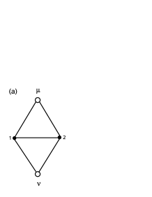
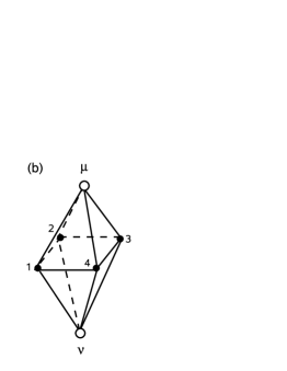
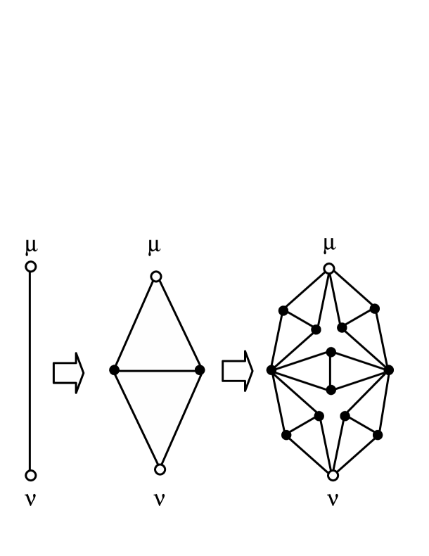
Hierarchical lattices were introduced within the context of the real-space renormalization-group (RG) approach, bringing the great advantage that such technique becomes exact for pure systems defined on these lattices tsallismagalhaes . These lattices are constructed by carrying successive similar operations at each hierarchical level, e.g., at each level one replaces bonds by well-defined unit cells; typical examples of unit cells are presented in Fig. 1, all of them belonging to the Wheatstone-Bridge (WB) family of hierarchical lattices. Two important characteristics of a given hierarchical lattice are its fractal dimension and its scaling factor , which is defined as the smallest distance (counted in bonds) between the two external sites of its basic cell. The WB hierarchical lattices are generated by starting the process from the th level of the lattice-generation hierarchy with a single bond joining the external sites (denoted by and ); then, in each iteration step one replaces a bond by its corresponding unit cell, in such a way that in its first hierarchy the lattice is represented by this unit cell. This procedure is shown explicitly in Fig. 2, for the first three levels of the WB hierarchical lattice with fractal dimension . The process is continued with the hierarchical lattice being constructed up to a given -th hierarchy ().
Although the RG may not be considered in general as an exact procedure for random systems on hierarchical lattices, it is expected to represent a good approximation, since in many cases, pure systems appear as particular limits of some random models. In the particular case of Ising SGs, the hierarchical lattices have been a very useful tool southernyoung ; braymoore87 ; banavar87 ; banavar88 ; curadomeunier ; niflehilhorst92 ; nobre98 ; drossel98 ; nogueira99 ; curado99 ; nobre00 ; drossel00 ; nobre01 ; nobre03 ; nishimoriberker ; salmonpre09 ; jorgkatzgraber1 , essentially due to the possibility of performing relatively low-time-consuming numerical computations. A significant gain in the computational time in the study of SGs represents the main advantage of the hierarchical lattices with respect to Monte Carlo simulations performed on Bravais lattices. In fact, one may obtain whole phase diagrams for non-symmetric distributions of the couplings (e.g., by changing the probability of a bimodal distribution) within typically, a few computation hours of a standard desk computer; on the other hand, the criticality of a given particular case (e.g., the study of the case of the bimodal distribution for the couplings) through Monte Carlo simulations may require several days on high-performance computer networks.
The Migdal-Kadanoff (MK) family of hierarchical lattices migdal ; kadanoff have been widely explored, essentially due to the fact that its basic cell is formed by one-dimensional parallel paths each with a given scaling factor ; its fractal dimension may be varied either by changing the scaling factor, or by a simple operation of adding more paths to the cell. As a consequence, most of the hierarchical-lattice SG studies so far were concentrated on these lattices southernyoung ; braymoore87 ; banavar87 ; banavar88 ; curadomeunier ; niflehilhorst92 ; drossel98 ; nogueira99 ; curado99 ; drossel00 ; jorgkatzgraber1 . In spite of its simplicity, some of the results obtained in these lattices are quite impressive: (i) The bounds for the lower critical dimension, which is accepted nowadays to be greater than 2, but smaller than 3, were obtained on MK lattices southernyoung about a decade before their confirmation through distinct numerical investigations bhattyoung85 ; ogielski85 ; bhattyoung88 ; braymoore87 . In fact, the lower critical dimension on MK lattices was estimated to be very close to curadomeunier ; (ii) The SG critical-temperatures on the MK hierarchical lattice of fractal dimension , for symmetric Gaussian and bimodal distributions southernyoung , present relative discrepancies of about , taking into account the error bars, when compared with the recent estimates from Monte Carlo simulations on a cubic lattice young06 .
However, the MK lattices represent the simplest types of hierarchical lattices and some of its results may be quantitatively poor approximations to well-known estimates on Bravais lattices. Other hierarchical lattices, which present connections between such parallel paths, may represent better approximations and in some cases, one may obtain precise estimates when compared to those known for Bravais lattices; this motivates the study of SG models on such lattices. In spite of this, only a few works have considered Ising SGs on hierarchical lattices different from those of the MK family nobre98 ; nobre00 ; nobre01 ; nobre03 ; nishimoriberker ; salmonpre09 and some of them have yielded important and stimulating results: (i) Studies on a special hierarchical lattice with fractal dimension led to an estimate for the stiffness exponent nobre98 (, where is the exponent associated with the divergence of the correlation length at zero temperature) in agreement with those obtained from other, more time-consuming, numerical approaches on a square lattice. An analysis of the Ising SG model nobre01 on the same hierarchical lattice gave a ferromagnetic-paramagnetic critical frontier that should be a good approximation for the one of the corresponding model on a square lattice; (ii) Estimates of locations of multicritical points for SGs on some non-MK hierarchical lattices are in very good agreement with other numerical results on Bravais lattices, as well as with a conjecture based on gauge theory nobre01 ; nishimoriberker .
In the present work we investigate Ising SGs defined on WB hierarchical lattices through the Hamiltonian,
| (1) |
The lattices generated by the cells shown in Figs. 1(a), (b), and (c) present fractal dimensions and ; one should remind that these cells may be obtained from simple constructions of parts of Bravais lattices, namely, the square, cubic and four-dimensional hypercubic lattices, respectively tsallismagalhaes . The denote random couplings between two spins located at nearest-neighboring sites and of this hierarchical lattice and may follow either the Gaussian, or bimodal () distributions,
| (2) |
| (3) |
Herein, we will restrict ourselves to those parts of the phase diagrams associated with ferromagnetic and SG orderings only, i.e., in Eq. (2), or in Eq. (3).
The RG procedure works in the inverse way of the lattice generation, i.e., through a decimation of the internal sites of a given cell, leading to renormalized quantities associated with the external sites. Defining the dimensionless couplings, [], the corresponding RG equations may be written in the general form,
| (4) |
where represent partition functions associated with the Hamiltonian for a given unit cell with the external spins kept fixed ,
| (5) |
The RG scheme is carried by following numerically the probability distribution associated with the the dimensionless couplings southernyoung . Operationally, this probability distribution is represented by a pool of real numbers ( is kept fixed throughout the whole RG procedure), from which one may compute its associated moments, at each renormalization step; in the limit these moments should approach those of the distribution associated with . The process starts by creating a pool with coupling constants generated according to one of the distributions of Eqs. (2) or (3), yielding an initial pool of dimensionless couplings, , for a given temperature. An iteration consists in operations, where in each of them one picks randomly a set of numbers from the pool (each number is assigned to a bond for a given cell in Fig. 1) in order to generate the effective coupling according to Eq. (4), which will correspond to an element of the new pool. Following this procedure, one gets a new pool with the same size of the previous one, representing the renormalized probability distribution. During the RG procedure, the average, , and the width, , are of particular interest for the identification of the phases, in such a way that one may obtain the Paramagnetic (P), Ferromagnetic (F), and Spin-Glass (SG) phases, as dominated by the attractors,
| (6) |
Strictly speaking, this procedure should be carried for many different initial pools of real numbers, over which one may compute sample averages. However, one may also get good critical-frontier estimates by analyzing a sufficiently large single pool; the results that follow were obtained by considering a single pool of size real numbers.
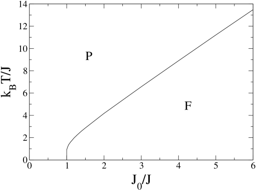
As expected, we did not find a finite-temperature SG phase for the hierarchical lattice defined by the unit cell of Fig. 1(a), for either one of the distributions of Eqs. (2) or (3). The phase diagram for the case of the Gaussian distribution for the couplings is exhibited in Fig. 3, where only two phases are present, namely, the P and F phases. The points used in order to draw this phase diagram were calculated from the standard narrowing RG procedure, with at least a two-decimal-digit certainty (error bars on third decimals). Due to the duality property of this unit cell tsallismagalhaes , one should obtain the exact critical temperature of the ferromagnetic Ising model on the square lattice from the phase diagram of Fig. 3; indeed, computing the slope of the critical frontier of Fig. 3 for large, one gets . Although this model does not exhibit a SG phase at finite temperatures, one may still compute the stiffness exponent , which rules the zero-temperature scaling behavior of the width of a continuous coupling distribution associated with blocks of linear size braymoore87 ,
| (7) |
For sufficiently small values of , the sign of the stiffness exponent is directly associated with the low-temperature phase; for a positive (negative) the system scales to strong (weak) couplings, characteristic of a SG (paramagnetic) state at low temperatures. Therefore, one expects for the WB hierachical lattice of Fig. 1(a), whereas one should get for those of Figs. 1(b) and 1(c). In the first case one may use the scaling relation, braymoore87 , for a phase transition in the limit , where is the exponent associated with the divergence of the correlation length, . We have computed , leading to , for all in the interval (cf. Fig. 3). This estimate coincides, within the error bars, with those obtained for the particular case in Ref. nobre98 for the same hierarchical lattice, as well as with several estimates for the square lattice, like braymoore87 , hartmann , and weigel . Although the lattice considered herein presents a fractal dimension , which is about higher than the dimension of the square lattice, it has been much used in the literature as an approach for models on the later, essentially because it may be obtained through a simple construction from a piece of the square lattice, keeping one of its most important properties, the self-duality tsallismagalhaes .
The phase diagram for the case of the hierarchical lattice defined by the unit cell of Fig. 1(a), with a bimodal distribution for the couplings, is qualitatively similar to the one already investigated in Ref. nobre01 . From the present analysis one concludes that the SG lower critical dimension in the WB hierarchical-lattice family should be greater than ; this result is in agreement with calculations carried on MK lattices, where this lower critical dimension was estimated to be very close to curadomeunier .
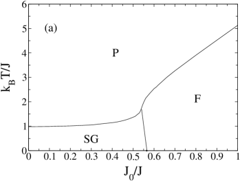
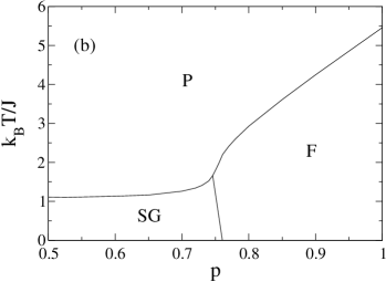
The phase diagrams for the hierarchical lattice defined by the unit cell of Fig. 1(b) are shown in Fig. 4, for couplings following the Gaussian distribution [Fig. 4(a)], or the bimodal distribution [Fig. 4(b)]. The coordinates of the most important critical points of these phase diagrams are given explicitly in Tables I and II. Similarly to the previous case, the points used in order to draw these phase diagrams were calculated from the standard narrowing RG procedure, with at least a two-decimal-digit certainty (error bars on third decimals). It is important to notice the estimates of the critical temperatures for symmetric distributions, namely, and ; these estimates are in very good agreement with recent results from Monte Carlo simulations on a cubic lattice, which yielded and , for symmetric Gaussian and bimodal distributions, respectively young06 . Comparing the present results with those of Ref. young06 , taking into account the error bars, one finds a relative discrepancy of about in the Gaussian case, whereas for the symmetric bimodal distribution the two estimates essentially coincide (leading to a relative discrepancy of about ). Such good agreements on critical-temperature estimates, between those of a hierarchical lattice with fractal dimension and those of the cubic lattice, are justified by the fact that the cell of Fig. 1(b) may be obtained from a simple construction of a piece of the cubic lattice tsallismagalhaes . On the other hand, the critical temperature associated with the corresponding ferromagnetic Ising model, which may be obtained either from the critical point separating phases P and F in Fig. 4(b), or by computing the slope of the critical frontier of Fig. 4(b) for large, is given by , which is somewhere in between the estimates of critical temperatures for the ferromagnetic Ising model on the cubic [] and the four-dimensional hypercubic lattice [, obtained from Monte Carlo simulations staufferbjp .
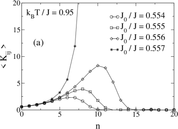
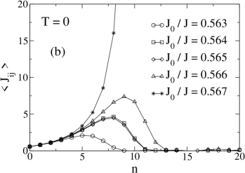
Another important aspect of the phase diagrams shown in Fig. 4 is a small reentrance effect in the region slightly to the right of the multicritical point; by lowering the temperature, one may go from a high-temperature disordered (P) phase to an ordered one (F phase) and then, back to a more disordered (SG) phase at low temperatures. By comparing the coordinates of the multicritical points and the respective zero-temperature ones in Tables I and II, one sees that this effect, although very weak, is outside the error bars of the method. This is illustrated in Fig. 5, which shows the evolution of the average with the RG step , in the case of couplings following an initial Gaussian distribution, for typical values of around the critical frontier separating the phases SG and F. In Fig. 5(a) one sees the behavior of for a fixed temperature [], below the SG critical temperature, showing that for one is still on the SG phase, whereas diverges for , signalling a F phase. The same procedure is applied to zero temperature in Fig. 5(b), where one sees these two different types of behavior for and , respectively. It should be mentioned that this type of reentrance phenomena has been observed experimentally, e.g., in malettaconvert and ( Fe) craneclaus . Theoretically, it has been also found in the mean-field replica-symmetric solution (which turns out to be unstable at low temperatures) of the Ising SG, although its correct solution, characterized by replica-symmetry breaking, has washed away the reentrance dotsenkobook ; nishimoribook ; parisirsb . It is important to stress that reentrance phenomena on theoretical SG models are very subtle and difficult to be obtained numerically, in such a way that only a few works in the literature were able to capture such an effect so far (see, e.g., Refs. nobre01 ; toldin ).
| Hierarchical | Multicritical Point | ||
|---|---|---|---|
| lattice | () | () | |
| Cell 1(b) | ; | ||
| Cell 1(c) | ; |
We have also computed the zero-temperature stiffness exponent for the phase diagram of Fig. 4(a). As expected, a positive value, , signals a SG phase at finite temperatures; furthermore, this estimate is universal for all values of within the SG phase. This value is close to the recent one obtained for a MK lattice of fractal dimension ( jorgkatzgraber1 ), but it is slightly larger than those for the cubic lattice, braymoore87 and jorgkatzgraber1 .
The phase diagrams for the hierarchical lattice defined by the unit cell of Fig. 1(c), for couplings following either initial Gaussian of bimodal distributions, are qualitatively similar to those shown in Figs. 4(a) and 4(b), respectively. Values of typical critical points in these phase diagrams are given explicitly in Tables I and II. The higher complexity of this lattice generates larger errors in the numerical estimates; however, the points in such phase diagrams were computed with at least a one-decimal-digit certainty (error bars on second decimals). In particular, one should mention the estimates of the critical temperatures for symmetric distributions, namely, and , which are about above those obtained from Monte Carlo simulations for the four-dimensional hypercubic lattice, i.e., , for the Gaussian distribution jorgkatzgraber2 , and , for the bimodal distribution hukushima , respectively. These overestimates are consistent with the fact that the fractal dimension of the lattice considered herein is well above four (). Although we are not aware of numerical simulations carried for Ising SGs on lattices of higher dimensions, the present estimate for the symmetric bimodal distribution is slightly below the one obtained through series expansions on the five-dimensional hypercubic lattice, klein .
| Hierarchical | Multicritical Point | ||
|---|---|---|---|
| lattice | () | () | |
| Cell 1(b) | ; | ||
| Cell 1(c) | ; |
To conclude, we have investigated nearest-neighbor-interaction Ising spin glasses defined on three different hierarchical lattices, belonging to a family of Wheatstone-Bridge lattices, characterized by fractal dimensions and . The interactions among pairs of spins were chosen from either a Gaussian, or a bimodal (), non-centered distribution. Through calculations of the stiffness exponent, we have shown that the spin-glass lower critical dimension in these lattices should be greater than . Finite-temperature spin-glass phases were found for the lattices of fractal dimension and . In the former case, whose hierarchical lattice is constructed as an approximation to the cubic lattice, the estimates of spin-glass critical temperatures associated with zero-centered Gaussian and bimodal distributions are very close to the most recent estimates from extensive numerical simulations carried on the cubic lattice. Phase diagrams were obtained for couplings following non-centered distributions – which are not entirely known, up to the moment, for spin-glass models on Bravais lattices – either for in the case of the Gaussian distribution, or in the case of the bimodal distribution; these phase diagrams are expected to represent good approximations for the corresponding models on Bravais lattices.
Acknowledgments
We thank Prof. E. M. F. Curado for fruitful conversations. The partial financial supports from CNPq and Pronex/MCT/FAPERJ (Brazilian agencies) are acknowledged.
References
- (1) V. Dotsenko, Introduction to the Replica Theory of Disordered Statistical Systems, Cambridge University Press, Cambridge, 2001.
- (2) H. Nishimori, Statistical Physics of Spin Glasses and Information Processing, Oxford University Press, Oxford 2001.
- (3) G. Parisi, Phys. Rev. Lett. 43 , 1754-1756 (1979); 50 (1983) 1946-1948.
- (4) E. Marinari, G. Parisi, and J.J. Ruiz-Lorenzo, in: A. P. Young (Ed.), Spin Glasses and Random Fields, World Scientific, Singapore, 1998, pp. 59-98.
- (5) B. W. Southern and A. P. Young, J. Phys. C 10 (1977), 2179-2195.
- (6) R. N. Bhatt and A. P. Young, Phys. Rev. Lett. 54 (1985), 924-927.
- (7) A. T. Ogielski and I. Morgenstern, Phys. Rev. Lett. 54 (1985) 928-931.
- (8) A. J. Bray and M. A. Moore, in: J. L. van Hemmen and I. Morgenstern (Eds.), Heidelberg Colloquium on Glassy Dynamics, Lecture Notes in Physics 275, Springer-Verlag, Berlin, 1987, 121-153.
- (9) R. N. Bhatt and A. P. Young, Phys. Rev. B 37 (1988) 5606-5614.
- (10) A. P. Young and H. G. Katzgraber, Phys. Rev. Lett. 93 (2004) 207203-1-207203-4.
- (11) H. G. Katzgraber, M. Körner, and A. P. Young, Phys. Rev. B 73 (2006) 224432-1- 224432-11.
- (12) T. Jörg, H. G. Katzgraber, and F. Krza̧kala, Phys. Rev. Lett. 100 (2008) 197202-1-197202-4.
- (13) T. Jörg and H. G. Katzgraber, Phys. Rev. Lett. 101 (2008) 197205-1-197205-4.
- (14) C. Tsallis and A. C. N. de Magalhães, Phys. Rep. 268 (1996) 305-430.
- (15) J. R. Banavar and A. J. Bray, Phys. Rev. B 35, 8888-8890 (1987).
- (16) J. R. Banavar and A. J. Bray, Phys. Rev. B 38 (1988) 2564-2569.
- (17) E. M. F. Curado and J. L. Meunier, Physica A 149 (1988) 164-181.
- (18) M. Nifle and H. J. Hilhorst, Phys. Rev. Lett. 68 (1992) 2992-2995.
- (19) F. D. Nobre, Phys. Lett. A 250 (1998) 163-169.
- (20) M. A. Moore, H. Bokil, and B. Drossel, Phys. Rev. Lett. 81 (1998) 4252-4255.
- (21) E. Nogueira Jr., S. Coutinho, F. D. Nobre, and E. M. F. Curado, Physica A 271 (1999) 125-132.
- (22) E. M. F. Curado, F. D. Nobre, and S. Coutinho, Phys. Rev. E 60 (1999) 3761-3770.
- (23) F. D. Nobre, Physica A 280 (2000) 456-464.
- (24) B. Drossel, H. Bokil, M. A. Moore, and A. J. Bray, Eur. Phys. J. B 13 (2000) 369-375.
- (25) F. D. Nobre, Phys. Rev. E 64 (2001) 046108-1-046108-6.
- (26) F. D. Nobre, Physica A 319 (2003) 362-370.
- (27) M. Ohzeki, H. Nishimori, and A. N. Berker, Phys. Rev. E 77 (2008), 061116-1-061116-11.
- (28) O. R. Salmon and F. D. Nobre, Phys. Rev. E 79 (2009) 051122-1-051122-6.
- (29) A. A. Migdal, Sov. Phys. JETP 42 (1976) 743-746.
- (30) L. P. Kadanoff, Ann. Phys. 100 (1976) 359-394.
- (31) A. K. Hartmann, A. J. Bray, A. C. Carter, M. A. Moore, and A. P. Young, Phys. Rev. B 66 (2002) 224401-1-224401-4.
- (32) M. Weigel and D. Johnston, Phys. Rev. B 76 (2007) 054408-1-054408-8.
- (33) D. Stauffer, Braz. J. Phys. 30 (2000) 787-793.
- (34) H. Maletta and P. Convert, Phys. Rev. Lett. 42 (1979) 108-111.
- (35) S. Crane and H. Claus, Phys. Rev. Lett. 46 (1981) 1693-1695.
- (36) F. P. Toldin, A. Pelissetto, and E. Vicari, J. Stat. Phys. 135 (2009) 1039-1061.
- (37) T. Jörg and H. G. Katzgraber, Phys. Rev. B 77 (2008) 214426-1-214426-12.
- (38) K. Hukushima, Phys. Rev. E 60 (1999) 3606-3613.
- (39) L. Klein, J. Adler, A. Aharony, A. B. Harris, and Y. Meir, Phys. Rev. B 43 (1991) 11249-11273.
Figure Captions
Fig. 1: Basic cells of the WB family of hierarchical lattices, with a scaling factor . In each case, the empty circles ( and ) represent the external sites of the cell, whereas the black circles are internal sites to be decimated in the RG procedure. (a) The WB cell of fractal dimension ; (b) The WB cell of fractal dimension ; (c) The WB cell of fractal dimension . For clearness, all the bonds of cell (c) are not shown explicitly; the external site is connected directly to sites and (as illustrated by the bond connecting sites and , whereas site is connected directly to sites and (as illustrated by the bond connecting sites and ).
Fig. 2: First three levels (levels and ) in the generation process of the Wheatstone-Bridge hierarchical lattice with fractal dimension . The lattice-generation process starts at the -th level with a single bond and at each step a bond is replaced by its respective basic cell. In each level, the empty circles ( and ) represent the external sites of the lattice, whereas the black circles are internal sites to be decimated in successive RG operations.
Fig. 3: Phase diagram for an Ising SG on the hierarchical lattice defined by the unit cell of Fig. 1(a), with a Gaussian distribution for the couplings.
Fig. 4: Phase diagrams of the Ising SG on the hierarchical lattice defined by the unit cell of Fig. 1(b): (a) Gaussian distribution for the couplings; (b) bimodal distribution for the couplings.
Fig. 5: Evolution of the average of couplings with the RG step , for the case of an initial Gaussian distribution, considering typical values of around the critical frontier separating the phases SG and F. (a) Fixed temperature below the SG critical temperature; (b) Zero temperature.