Numerical Regularized Moment Method of Arbitrary Order for Boltzmann-BGK Equation
Abstract
We introduce a numerical method for solving Grad’s moment equations or regularized moment equations for arbitrary order of moments. In our algorithm, we do not explicitly need the moment equations. Instead, we directly start from the Boltzmann equation and perform Grad’s moment method [12] and the regularization technique [27] numerically. We define a conservative projection operator and propose a fast implementation which makes it convenient to add up two distributions and provides more efficient flux calculations compared with the classic method using explicit expressions of flux functions. For the collision term, the BGK model is adopted so that the production step can be done trivially based on the Hermite expansion. Extensive numerical examples for one- and two-dimensional problems are presented. Convergence in moments can be validated by the numerical results for different number of moments.
Keywords: Boltzmann-BGK equation; Grad’s moment method; Regularized moment equations
1 Introduction
In recent years, the simulation of rarefied fluids or microflows, which contain significant non-equilibrium characteristics, became one of the major directions of fluid dynamics. The Boltzmann equation, which is considered as the basis of modern kinetic theory, is the starting point of such simulations. Because of the high dimension of variables and the complicated form of its collision operators, people tend to use its discrete or simplified form instead of the Boltzmann equation itself in numerical simulation. Lots of work has been done to simplify the collision operator, such as the BGK model [4], the Shakhov model [23], the ES-BGK model [17], the Liu’s model [18], the Maxwell molecules model [11], and so on. Another way of simplification is to discretize the Boltzmann equation by some expansion. In this field, the Chapman-Enskog expansion [8, 10] and the Grad’s expansion [12, 14] achieved great success in the early exploration of kinetic theory.
However, both methods of expansion suffer some problems which greatly restrict their application. The Chapman-Enskog expansion shows an unstable behavior in the case of high order expansions, such as Burnett and super-Burnett equations [5]; the Grad’s moment equations lead to unphysical subshocks when the Mach number is large (see e.g. [26]). In order to extend their use, several corrections are applied to these models, which include the R13 model, proposed by H. Struchtrup and M. Torrilhon in [27]. The regularization of Grad’s moment equations is done by combining Grad’s technique with first-order Chapman-Enskog expansion. [38] summarizes the recent work on R13 equations, in which it is mentioned that such a regularization technique can be extended to any system obtained by Grad’s moment method. In this paper, we introduce a method that numerically solves the Grad’s equations for arbitrary order of moments together with their regularization. The numerical method generating the Grad’s moment equations for arbitrary number of moments has been proposed in [34] and implemented in [2]. And the results for shock tube are reported in [33, 3]. However, we solve these equations “only numerically,” which means we do not need the explicit forms of those equations in our algorithm. The regularized moment equations are also considered, and to our knowledge, no results about the generation of regularized equations for arbitrary number of moments have been reported. Numerical methods for R13 equations are discussed in [32, 15, 37], and the computational framework for the R20 equations can be found in [21].
Our starting point is the Boltzmann equation, and we adopt the BGK model and a uniform rectangular mesh for discretizing the spatial variable for simplicity. The distribution function is expanded in an Hermite series using the method in [12]. The series is truncated at a certain place and the coefficients in the expansion are stored for each cell. Following the standard procedure, we adopt the classic time splitting method in our scheme. The convection term of the Boltzmann equation is discretized by the finite volume method with the HLL numerical fluxes. This requires algebraic operations on the distributions between the neighbouring cells. Grad’s method expands the distribution function by the Hermite functions with center at the local mean velocity and a scaling factor associated with the local temperature, while these parameters are different in different places. This makes it nontrivial to add up two distributions in different cells. Thus it is extremely complicated to calculate the numerical fluxes directly. As a key technique in this paper, we propose a fast algorithm which projects a distribution function expanded in the discrete space with one mean velocity and macroscopic temperature to that with another mean velocity and macroscopic temperature. This projection is conservative with respect to all the moments that are not truncated. Moreover, we prove the projection is invertible so that no information will be lost. With the help of this fast projection, distributions in any two neighbouring cells can be transformed into the same space efficiently. In order to estimate the signal velocities in the HLL numerical fluxes, we prove that the eigenvalues of the Jacobian matrix of the linearized flux function are actually the roots of Hermite functions plus the mean velocity. Thus we can take the eigenvalues with maximal absolute values as the approximated signal velocities. Now, standard HLL numerical fluxes can be calculated conveniently. After accumulating the contribution of the convection term, the expansion is not of Grad’s type any more, since Grad’s expansion requires all first-order coefficients and the trace of second-order coefficients to be zero. Again, the fast projection is applied to correct the center and scaling factor of the expansion so that the properties of Grad’s expansion can be recovered. These properties make it trivial to perform production of the BGK model by a direct scaling of the moments with orders not lower than two.
In [27], H. Struchtrup and M. Torrilhon used the Chapman-Enskog expansion to deduce the regularized system of Grad’s 13-moment equations — R13 equations. The basic idea of this regularization can be viewed as a strategy to “guess” the truncated moments. Using this idea, we apply the Chapman-Enskog expansion of the Boltzmann equation around the Grad non-equilibrium manifolds [26] of arbitrary order. The closure of the system is then achieved by the standard asymptotic techniques therein. This method can be perfectly integrated into our numerical scheme without deducing the macroscopic equations by intricate algebraic calculations. For arbitrary order of moments, the regularization in our algorithm introduces only first order derivative terms, which can be numerically approximated by gradient reconstruction.
In our method, the computational cost of the fast conservative projection is linear in terms of the number of moments. Thus it is essentially faster to calculate the numerical fluxes than the classic method using the flux functions in the macroscopic equations. Actually, the macroscopic equations have never been deduced, but they have been solved implicitly by our method. Then the framework of our method can appear to be uniform for moment equations of any order. This makes it very convenient to implement our algorithm. We need not deduce and code for the complicated flux functions at all in the case of high order. Moreover, we need only to develop one copy of the code for all different orders.
We carry out numerical experiments in both one- and two-dimensional cases. Different Knudsen numbers and different orders of moments are examined to demonstrate the usefulness of large moment systems, and the convergence in moments is validated numerically. Regularized moment systems ranging from 20 moments up to 455 moments are simulated in our one-dimensional examples. Two-dimensional examples for up to 84 moments are presented, and there is even an example demonstrating the capacity of our method to simulate a three-dimensional non-equilibrium process. To the best of our knowledge, it is the first time that the method for arbitrary order regularized moment equations is numerically implemented, and the moment method for large systems are applied to two-dimensional problems.
The layout of this paper is as follows: in Section 2, an overview of Boltzmann equation and the BGK model is given as the basis of our algorithm. In section 3, the details of the algorithm which generate numerical solution for arbitrary order Grad’s moment equations are introduced. In section 4, regularization of moment equations is considered and then the whole algorithm is outlined. We present in Section 5 four numerical examples including one- and two-dimensional tests to make a comparison between results for different moment equations, different Knudsen numbers and different meshes. At last, some concluding remarks will be given in Section 6.
2 The Boltzmann equation and BGK collision model
In the kinetic theory of gases, the flow of a dilute gas is described by the Boltzmann equation (see e.g. [7, 9, 26])
| (2.1) |
where is the distribution function, and . is the collision term with a quadratic expression given by
| (2.2) |
where
| (2.3) |
and and are velocities after collision of two particles with original velocities and and with unit vector joining the centers of them. is a constant equivalent to , which keeps invariant when taking Boltzmann-Grad limit , (cf. [7, 9]). Here is the number of particles while is the diameter of each particle.
However, such a collision term turns out to be too complicated for numerical simulation, so a variety of variants are raised to get it simplified. To some extent, the BGK operator [4] is the simplest one. It substitutes the collision term by
| (2.4) |
where is the collision frequency, and is the local Maxwellian defined as
| (2.5) |
It is related with by
| (2.6) |
where and can be viewed as macroscopic variables density, velocity and temperature, respectively. This model is much more easy to use in numerical methods. However, it suffers the disadvantage of being unable to predict the correct Prandtl number, which will be seen in the numerical tests.
3 A numerical formation equivalent to Grad’s moment method
3.1 Discretization of the distribution function
In order to solve the kinetic equations numerically, we first expands the distribution function into Hermite functions as in [12]:
| (3.1) |
where is a -dimensional multi-index, and
| (3.2) |
The basis functions are chosen as
| (3.3) |
where is the Hermite polynomial defined by
| (3.4) |
Note that this is formally inconsistent with Grad’s original expression, but will be more convenient for our deduction below111Grad uses symbols as to denote basis functions. This symbol is equivalent to which is used here, where is a constant factor. Inversely, can be expressed as with ones, twos, , and ’s in the subscript . Thus our expansion is actually the same as what Grad has done.. The properties of Hermite polynomials can be found in many handbooks such as [1]. Some useful ones are listed below:
-
1.
Orthogonality: ;
-
2.
Recursion relation: ;
-
3.
Differential relation: .
It can be derived from the recursion relation and the differential relation that
| (3.5) |
The expansion (3.1) together with (2.6) yields
| (3.6) |
where stands for the multi-index with the th component and all other components .
It is known that (3.1) will result in an “infinite moment system”. In order to make it numerically solvable, we choose a positive integer and approximate (3.1) by
| (3.7) |
Using to denote the linear space spanned by all ’s, where and is defined by (3.2), then is a finite dimensional subspace of .
Remark 1.
Remark 2.
The definition of (eq. (3.2)) implies that we take the mean velocity as the “origin” and as the scaling factor when discretizing the distribution function. Thus (3.6) holds. If (3.6) is violated, and we suppose , , and a distribution function is approximated as
| (3.10) |
with ’s or nonzero, then the associated and can be calculated by substituting (3.10) into (2.6). Since
| (3.11) |
employing the orthogonality of Hermite polynomials, the integrals on the right hand sides of (2.6) can be directly worked out as
| (3.12) |
Tölke, Krafczyk, Schulz and Rank [29] use in their discretization. Additionally, the heat flux can be calculated by
| (3.13) |
3.2 Outline of the fractional step method
In this subsection, our numerical scheme will be outlined. Suppose and . is a uniform rectangular mesh in , with all grid lines parallel with the axes, and each cell is identified by an -dimensional multi-index . That is, for a fixed and ,
| (3.14) |
Using to approximate the average distribution function over the cell at time , the Boltzmann equation (2.1) can be solved by a standard fractional step method:
-
1.
Convection step:
-
2.
Production step: .
In the convection step, the finite volume method is employed and is the numerical flux between cell and . In the production step, is a transform over , and is considered as an approximation to . Here and are the mean velocity and temperature corresponding to the distribution function .
The numerical flux can be chosen from the standard ones in the finite volume method, but in our framework, only central schemes are available since the characteristic factorization of the flux function is not available yet. A series of central schemes can be found in textbook [30], and we choose the HLL scheme [16] in our numerical experiments, which reads
| (3.15) |
and are the fastest signal velocities arising from the solution of the Riemann problem, which will be discussed in Section 3.3.2. For all , given
| (3.16) |
where , and are the mean velocity and temperature in cell , then can be calculated according to the recursion relation of Hermite polynomials:
| (3.17) |
Since when , no longer exists in the space . Thus, we need an additional “projection step” to drag (3.17) back into . This can be done by simply dropping the terms with , since when , is orthogonal to with respect to the inner product
| (3.18) |
However, the convection step is still uncompleted since it is nontrivial to add up two functions lying in and respectively. This is a part of our major work and will be discussed in 3.3.
As to the production step, the main job is to construct the numerical collision operator . This is also implemented by projecting into . Precisely, is defined as
| (3.19) |
where
| (3.20) | |||
| (3.21) |
Further calculation requires the concrete forms of and in (2.3). For BGK model (2.4), the numerical collision operator has a simple explicit form (3.9). In this situation, all ’s can be decoupled, so the production step can be performed by solving each analytically. The scheme reads
-
2.
Production step (only for BGK model):
Remark 3.
For the time integration, we use a single step Euler scheme for both convection and production step. Actually, such formation can be smoothly generalized to Runge-Kutta and Strang splitting schemes.
Remark 4.
For other collision terms, such as ES-BGK model [17] or Maxwell molecules [11], the expression of can be much more complicated. For the ES-BGK model, it is always possible to get ’s by direct integration. For Maxwell molecules and linearized Boltzmann collision operator, the method in [34] can be employed to generate the numerical collision operator . For simplicity, these models are not considered in this paper.
3.3 Completion of the convection step
Two points remain unclear for the convection step. One is that we need to find a way to add up two functions in different spaces and , so that it is applicable to calculate the numerical fluxes and to accumulate them to the solution at the last time step. And the other is the estimation of the characteristic velocities and .
3.3.1 Projection between two different spaces
Assume and . Obviously, when or , direct calculation of is inapplicable. Therefore, we want to find such that is some approximation of in . In order to realize such transformation, we propose a fast projection method which has a time complexity of below.
First, let us consider the case of , and . Then, has the following two representations
| (3.22) |
and
| (3.23) |
Suppose all ’s are known, and we want to solve all ’s. Let and . It is obvious that
| (3.24) |
Joining (3.22) and (3.23), we have
| (3.25) |
Now we introduce an auxiliary function , defined as
| (3.26) |
which satisfies
| (3.27) |
Comparing (3.26) (3.27) with (3.25), it can be found that for any , is just which is to be solved. Moreover, if we suppose
| (3.28) |
then an infinite ordinary differential system of can be obtained.
The detailed calculation of can be found in Appendix B, and we only show the final result here:
| (3.29) |
where
| (3.30) |
and the parameter of is . As required in (3.28),
| (3.31) |
must hold. (3.31) is an infinite system, but for any , if we consider only a subsystem containing all equations with , it is still closed. Therefore, in order to project a function into , it is only needed to solve (3.31) for all .
For an arbitrary function which is defined on , its projection to is defined as
| (3.32) |
See (3.21) for the definition of . The following proposition provides an algorithm to project a function in to .
Proposition 1.
Suppose can be represented by
| (3.33) |
For some and , satisfies
| (3.34) |
where and are given by (3.30), and . Let
| (3.35) |
Then and satisfies
| (3.36) |
Proof.
Let and
| (3.37) |
Thus forms a complete basis of . It follows that for an arbitrary set of , there exists a function , such that
| (3.38) |
When , a zero extension of onto gives that
| (3.39) |
holds for all , . Let . Since has a compact support on , we have . Now (3.39) and the orthogonality of Hermite polynomials implies that if
| (3.40) |
then for all , .
The preceding analysis shows that if
| (3.41) |
then for all , . Employing the orthogonality of Hermite polynomials again, we can deduce that for any ,
| (3.42) |
Thus (3.36) is established. ∎
Based on this proposition, the projection requires to solve an ordinary differential system (3.34). Let row vectors and be
| (3.43) |
and
| (3.44) |
Thus the ordinary differential equations (3.34) can be simplified as
| (3.45) |
Eq. (3.34) reveals that is an upper triangular matrix with vanished diagonal entries. Therefore, (3.45) can actually be solved by recursive integration. However, the direct integration will leads to calculations, so we solve (3.45) by applying steps of Runge-Kutta numerical integration, which is unconditionally stable due to the special form of . Since is sparse, each Runge-Kutta step costs only calculations. Thus the whole projection has a time complexity of .
Now let us return to the convection step. Using to denote the operator that projects any function to the space , then the convection step is described as following:
-
1.
Convection step:
-
(a)
Apply the convection within :
(3.46) -
(b)
Use (3.12) to calculate the mean velocity and temperature for the distribution function ;
-
(c)
Let , , and .
-
(a)
When implementing Step 1a, is actually applied on each term of , and the result no longer satisfies (3.6). So the mean velocity and temperature need to be recalculated in Step 1b. In Step 1c, is adjusted to such that (3.6) holds for . Later on, in the production step, the mean velocity and temperature are not changed, so (3.6) still holds for . The conservation of the convection step follows from proposition 1 and the conservative form of the finite volume scheme. To be specific, for any , we have
| (3.47) |
Thus quantities such as mass, total momentum and total energy are conservative.
3.3.2 Estimation of the characteristic velocities
In order to estimate and that are used in (3.15), we need to investigate into the expression of numerical flux carefully. Precisely, we should make sure the Riemann problem that such a numerical flux solves. In order to simplify the notation, we consider only the following form:
| (3.48) |
where and , and both satisfy (3.6). For which satisfies (3.6), is the projection operator from to , which simply discards the terms with orders higher than . is the projection operator from to . Then if we take
| (3.49) |
is exactly the same as in the case of . Similarly, let
| (3.50) |
Then is just if and in the case of . Due to the similar forms of and , only is considered below.
The nature of can be depicted with the help of the following proposition:
Proposition 2.
is invertible.
Proof.
Denote the projection operator from to as . We are going to prove that is the identity operator. Proposition 1 shows that for any and ,
| (3.51) |
That is,
| (3.52) |
Choosing for , respectively, and making use of the orthogonality of Hermite polynomials, it follows that
| (3.53) |
Similarly, it can be proved that is also the identity operator. Thus is invertible. ∎
Now let us turn back to the numerical flux (3.48). Let . Based on proposition 2, we rewrite (3.48) as
| (3.54) |
where is the projection from to itself, which is actually the identity operator. Now it is clear that the corresponding Riemann problem of is
| (3.55) |
Here always lies in , and the meanings of and have been changed a little. Suppose and are the mean velocity and temperature associated with , whose explicit expressions can be obtained from (3.12). Then is defined as the projection operator from to , and is defined as the projection operator form to .
The characteristic velocities of Riemann problem (3.55) seem to be difficult to obtain. Therefore, in order to give an estimation of and , we choose a fixed distribution function that lies “between” and , and linearize (3.55) as
| (3.56) |
Thus, we only need to estimate the eigenvalues of , which is an operator on . Since is linear and invertible, the problem can be further simplified as the estimation of eigenvalues of , which is an operator on . Taking , we have
| (3.57) |
For the eigenvalues of , we have the following proposition:
Proposition 3.
The eigenvalues of are formed by all the zeros of , .
Proof.
Suppose , and all zeros of are denoted as . Note that all ’s are real and different (see e.g. [25]), so we can assume that
| (3.58) |
For any , there exists a unique polynomial that satisfies , . Let satisfy and . We are going to prove
| (3.59) |
The definition of shows
| (3.60) |
where is a properly selected constant such that (3.60) lies in . Thus, for any and satisfying , we have
| (3.61) |
Then (3.59) holds due to the uniqueness of .
It remains to prove that has no other eigenvalues. Let us count how many eigenvectors are included in the form of . Consider an arbitrary and . Let
| (3.62) |
Obviously and satisfy and . Thus each uniquely determines an eigenvector. However, the number of such ’s are equal to the dimension of space , so has no other eigenvectors, thus no other eigenvalues, either. ∎
According to Proposition 3, the smallest and largest eigenvalues of are the smallest and largest zeros of , denoted by and . (3.57) shows that the smallest and largest eigenvalues of are and respectively. Since lies “between” and , we use
| (3.63) | |||
| (3.64) |
while computing numerical fluxes. In our implementation, we use the subroutine in ALGLIB [6] to calculate the roots of , and and are also used in the CFL condition to determine the time step length.
Remark 5.
The numerical method described in this section is only of the first order. In order to extend it to higher order schemes, reconstruction techniques need to be added to the finite volume scheme. Since addition and subtraction between two distribution functions are already available, it is only needed to determine a proper “slope”, which can probably be done with the help of the standard slope limters used in the normal finite volume schemes.
3.4 Relation with the Grad-type moment method and the LBE model
The relation and difference between the Grad-type moment method [12, 14] and the LBE (lattice Boltzmann equations) model [28] are summarized in [24], where both models are considered to be some approximation to the Boltzmann equation by an Hermite polynomial expansion. The expansion (3.1) and truncation (3.7) are exactly the same as what have been done by Grad [12], which means the method described above is actually solving the Grad-type moment equations. For and , it corresponds to the -moment equations which take the complete th order moments. However, systems such as -moment equations are not included. Those complete th order moment equations are popular in extended thermodynamics, see e.g. [22, 33, 3]. A software called [2] is developed by J. Au, H. Struchtrup and M. Torrilhon to generate equations for arbitrary order of moments, however, explicit moment equations, when written in conservative form, require calculations for the flux function, and this is reduced to in our numerical formation.
Now that our numerical strategy is equivalent to Grad’s moment method, one can refer to [24] for the precise difference between our method and the LBE model. According to [24], the linearized equation (3.56) can be interpreted as the LBE model, which places the center of the lattice at . Thus such linearization is reasonable.
4 Regularization of the moment method
The main drawback of Grad’s moment method is that its hyperbolicity yields unphysical subshocks [13]. The behavior in the case of high order moment equations can be found in [33, 3]. [14] provided a way to regularize Grad’s moment equations, and it was further studied in [27, 36] as R13 equations. Now we follow the regularization technique in [27] and regularize the numerical method introduced in Section 3 in exactly the same way.
4.1 Chapman-Enskog expansion around the truncated distribution
Independent of Grad’s method, Chapman-Enskog expansion [8, 10] is another important method for deriving equations of macroscopic variables. Following the generic procedure of Chapman-Enskog expansion, a scaling parameter is introduced on the right hand side of the Boltzmann equation. However, according to [27, 26], only the high order part instead of the whole collision term is scaled:
| (4.1) |
where is a truncation of the distribution function (3.1) defined by
| (4.2) |
The scaled part will be denoted as below. Let us apply the Chapman-Enskog expansion around , i.e. expand by
| (4.3) |
and we require that the truncation at any term of this expansion keeps the same values of all the moments with orders less than or equal to . Suppose the scaled part of the collision term has a corresponding expansion
| (4.4) |
It is reasonable to assume that has no zeroth order term since it has been taken away from . Match the zeroth order term on both sides of (4.1), and we have
| (4.5) |
For any multi-index with , multiplying on both sides and then integrating the whole equality over with respect to , since
| (4.6) |
the orthogonality of Hermite polynomials leads to
| (4.7) |
where
| (4.8) |
Now the concrete form of the production term is required for further calculation. Still, we adopt the simplest BGK model, which gives
| (4.9) |
Thus the second term on the right hand side of (4.7) also vanishes, and (4.7) becomes
| (4.10) |
This shows that can be represented as
| (4.11) |
where the coefficient is the corresponding coefficient of ’s expansion in .
At last, we set and approximate by . Since can be obtained from which is of finite dimension, when substituting such into the Boltzmann-BGK equation, a closed system can be obtained without more truncations. For and , the R20, R35, R56 equations for the BGK model can be obtained.
4.2 The numerical method
In this subsection, we restrict our focus on the BGK model. As in Section 3, only is stored at each time step. Note that for the BGK model, and are decoupled in the production step, which can be implemented exactly the same as that in Section 3. Therefore, we concentrate only on the convection step below.
Consider the original form of the numerical flux (3.15), and now is recognized as , where
| (4.12) |
The latter equation follows from (4.11), (3.32) and the orthogonality of the Hermite polynomials. Similarly, we have
| (4.13) |
Since only is desired after the convection step, the form of (3.46) is still adoptable. Therefore, we can mimic (3.48) and write the numerical flux as
| (4.14) |
where , , and . As described in Section 3, is just the flux for Grad’s moment equations. As to , (3.17) and (4.11) show
| (4.15) |
It is easy to see that in the expansions of and , only the coefficients with have effect on the numerical flux . We can also find that when , in (4.14) has actually no contribution to the velocity and temperature for the next time step, since (4.15) reveals that the Grad’s expansion of contains only terms with orders higher than or equal to , but (3.12) tells that and are only relevant with the coefficients with orders less than or equal to . That is to say, for all ’s, and can be solved using the method introduced in Section 3, without adding the “regularizing part of numerical flux” . Thus, the time derivative in (4.8) can be explicitly approximated by
| (4.16) |
Now, in order to approximate , it is only needed to approximate
| (4.17) |
For a fixed point , we have
| (4.18) |
where is defined by (3.21), and are the mean velocity and temperature at point , and is the projection operator to the space . Now consider the discrete circumstance. For each , can be obtained according to (3.17) and (3.34). Without confusion, the superscript “” will be omitted below, and is simplified as . Mimicing the method in [32], suppose
| (4.19) | |||
| (4.20) |
and then we can reconstruct the spatial partial derivative by a central difference in the smooth case:
| (4.21) |
or the van Leer reconstruction in the discontinuous case:
| (4.22) |
Thus we have
| (4.23) |
where (3.17) has been incorporated into the expression of .
From (4.15), we can conclude that
| (4.24) |
which appears twice on the right hand side of (4.14). This expression can be computed cheaply since has only non-zero coefficients. The last term in (4.14) requires us to compute
| (4.25) |
i.e. to apply another projection to the result of (4.24). Note that does not appear on the right hand side in (3.34), and for all , , the coefficients of in the expansion of (4.24) are zero, so all coefficients do not change after projection, saying if
| (4.26) |
then
| (4.27) |
This is the reason why a coefficient is multiplied in the definition of basis functions (3.3). Until now, the calculation of numerical fluxes for the regularized moment equations is thoroughly clarified.
Remark 6.
Remark 7.
As is known, the regularized moment equations contain second order derivative terms, so the CFL condition for the method above is
| (4.28) |
where is the maximum of and on all cells, and is the maximal collision frequency. Note that for this regularized model, when calculating and using (3.63) and (3.64), the roots of should be replaced by the roots of since we use the -th order moments of . Eq. (4.28) leads to a relatively small time step length. The time step length can be enlarged following the methods in [39, 32, 35], which is not yet implemented in our program.
Remark 8.
In our implementation, the classical fourth-order Runge-Kutta method is used to solve (3.34). Since the solution of regularized moment equations is generally smooth, most of the time, only one Runge-Kutta step is able to provide enough accuracy for such local projections. In the case of sharp initial values, some more steps are performed. However, such a situation only appears at the very beginning of the calculation.
4.3 Outline of the algorithm
As a summarization, our numerical method for the regularized moment equations is outlined as below:
-
1.
Let and set the initial state for all ’s.
-
2.
Determine the time step length according to the CFL condition (4.28).
-
3.
Apply the convection step in Section 3.
-
4.
Obtain as in Section 4.2.
-
5.
Add the “regularizing part of numerical flux” to .
-
6.
Apply the production step at the end of Section 3.2.
-
7.
Let , and return to step 2.
4.4 Boundary conditions
Currently, boundary conditions are not available in our numerical scheme. The boundary condition is always a delicate issue in the deduction of the macroscopic equations. Generally speaking, the kinetic boundary condition introduced by Maxwell [19] is expected to be added to the algorithm. As in [12] and [37], half-space integration needs to be performed during the construction of the distribution function in the ghost cells. This is possible to obtain for the discrete distributions , thanks to the recursion relation of the Hermite polynomials, but such integration requires a subroutine with a time complexity of , which results in much more computational time on the cells next to the wall. The details are still in preparation.
5 Numerical examples
In this section, 1D and 2D numerical examples of our method for the regularized moment equations are presented. In all these tests, the global Knudsen number is denoted as , and the collision frequency (see (2.4)) is substituted by . The CFL number is always . We use the POSIX multi-threaded technique in our simulation, and at most CPU cores are used.
5.1 One dimensional case
Two 1D examples are studied as follows. Since the boundary conditions are currently out of our consideration, only free or periodic boundary conditions are used in the following examples. In this section, some numerical solutions of the Boltzmann-BGK equation are provided, which are obtained according to the algorithm described in [20].
5.1.1 Shock tube test
The shock tube test has been investigated in many works due to its fundamental role in characterizing the hyperbolicity of equations. For Grad’s 13-moment system, it is shown in [31] that unphysical subshocks can be found. However, in [32], the numerical result of the Riemann problem shows that R13 equations are able to capture these waves correctly. Here we first repeat this test in [32] to obtain similar results.
As in [32], the initial conditions are
| (5.1) |
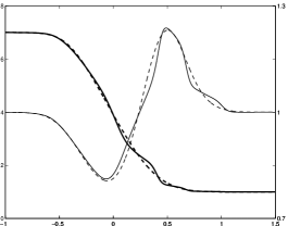
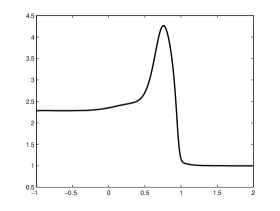
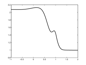
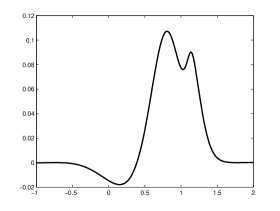
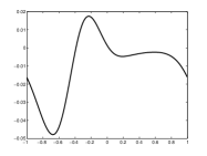
where the pressure equals to . The velocity is zero everywhere, and the fluid is in equilibrium everywhere. The computational domain is . In order to make a comparison, we set and compute this model until as in [32]. The result of R20 equations () is given in Figure 1. Compared with the result in [32], the plot of density agrees with that in [32] very well. The plot of heat flux has a similar shape with that in [32], but they differ in magnitude. This is due to the different models in the collision operator. The BGK model fails to predict the correct Prandtl number, which results in the incorrectness of heat flux.
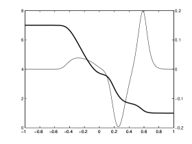
Since is small, almost the same results are produced by and no subshocks are found. This illustrates the capability of our method in capturing physical waves. Note that the peak and valley of the heat flux lies in the “discontinuities” of the density, which indicates the non-equilibrium. The negative part () has smaller heat flux due to the larger density or collision term.
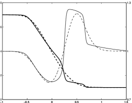
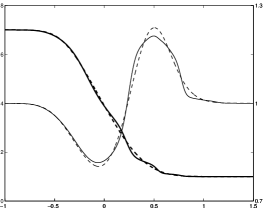
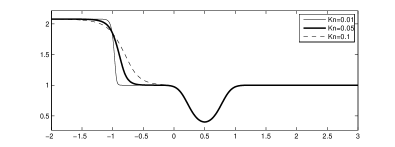
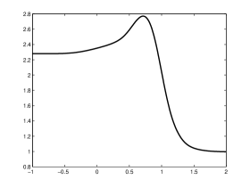
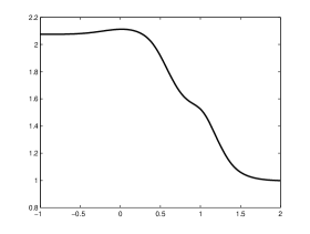
Now we set to investigate the numerical behavior of our method in the case of greater Knudsen number. The curves of density and temperature for to , as well as the numerical solutions of the Boltzmann-BGK equation, are plotted in Figure 2. With this Knudsen number, the hyperbolicity of the regularized moment equations clearly turns to be dominant. The solutions in Figure 2 exhibit a similar behavior with those in [33]. In the region of , all results are similar because of the high density behind the initial shock. In front of the initial shock, both the density and temperature are converging to the BGK solution, although the convergence rate is much slower.
5.1.2 A test with smooth initial values
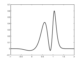
This example is again from [32]. The initial conditions are
| (5.2) |
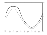
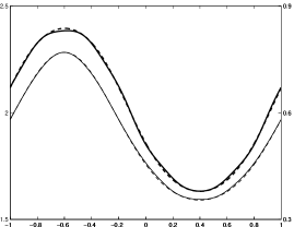
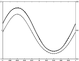
and the fluid is in equilibrium everywhere with . Periodic boundary condition is used and the computational domain is the interval . In order to validate our method, we use in our numerical computation exactly as in [32]. The end time is .
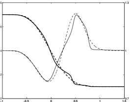
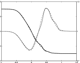
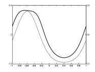
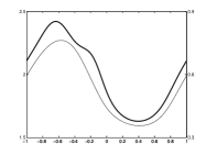
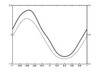
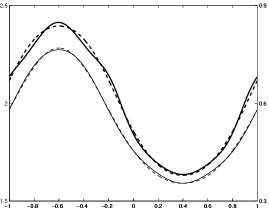
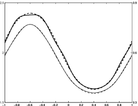
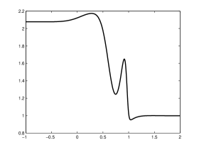
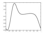
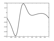
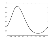
The results for different Knudsen numbers and different moment equations are plotted in Figure 3. All tests are computed using grids. The results in the first column are almost identical, which indicates the correct behavior of our method in the dense limit. The R20 equations, which should be the closest to the R13 system, produce similar results as those of R13 reported in [32]. The temperature plots in the first row can be used to make comparison.
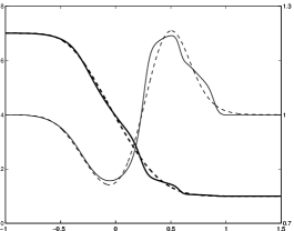
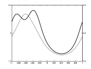
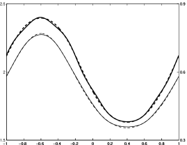
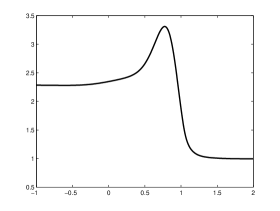
The new results are presented in the second and third columns, where the numerical solutions for high-order moment equations are listed. For , the R20 result shows an incorrect profile of density. With increasing , both the density and the temperature tend to converge. For , the R20 equations provide completely wrong structures, although smooth initial values are used. Results for even larger moment systems are plotted in Figure 4. In this plot, the satisfying temperature plot is obtained when , but the density plots behave similarly as those in Figure 2. The curves for odd and even order of moments hold different profiles, and they are toddling close to each other gradually. With been increased up to , the density curve eventually exhibits a satisfying convergence. The phenomenon illustrates the necessity of large moment systems in the microcase.
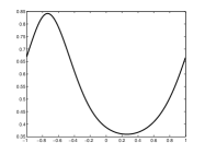
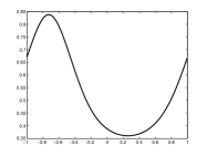
| R20 |  |
 |
 |
|---|---|---|---|
| R35 |  |
 |
 |
| R56 |  |
 |
 |
| R84 | 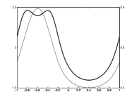 |
 |
 |

5.2 Two dimensional case
Two 2D examples are investigated in our numerical simulation. Both examples use uniform grids in the spatial discretization. Though much more computational cost are needed for 2D problems, the equations with up to 84 moments are considered.
5.2.1 Shock-bubble interaction
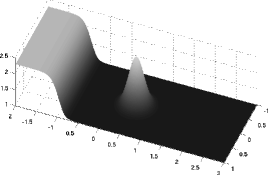
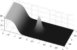
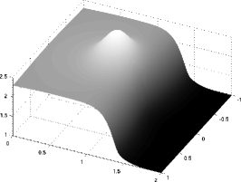
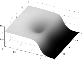
In this section, the shock-bubble problem tested in [32] is repeated. The initial state contains a shock wave at travelling with Mach number into an equilibrium area with . A bubble is in front of the shock with density profile
| (5.3) |
where , and constant pressure . The shock wave has a fully developed structure instead of a discontinuity. Thus a pre-computation of the shock profile is needed. The initial density surfaces for and are shown in Figure 5. A uniform mesh with grids is used in our numerical simulation.
The shock structure can be obtained by solving a 1D Riemann problem constructed according to the Rankine-Hugoniot condition. The left state is
| (5.4) |
and the right state is
| (5.5) |
Both states are in equilibrium. After a sufficiently long time, a stationary shock will form. It is quite convenient to transform a stationary shock to an unstable one in our numerical framework. Suppose a 1D steady shock is presented by
| (5.6) |
and it satisfies (3.6). Then, for an arbitrary velocity , let
| (5.7) |
Substituting and by and in (5.6) and keeping all the coefficients unchanged, then (5.6) becomes an unsteady shock travelling with speed . Let , and then the desired shock wave can be generated. The initial values of for , and at are plotted in Figure 6.
This example is aimed at the validation of our algorithm in the 2D case. To make comparison with the results in [32], , and are considered and only the R20 equations are simulated since it is the closest moment system to R13. Results for the dense case at are shown in Figure 7. Comparing with the results in [32], the profile exhibits a qualitatively agreement while the peak value between and disagrees. This is believed to be caused by the highly dissipative numerical flux without gradient reconstruction in our implementation. For , our R20 results of density and temperature (Figure 8) are much closer to those presented in [32]. But again, the heat fluxes show the same profile with different magnitude, owing to the BGK model used here. The whole structure after interaction with the bubble is drawn in Figure 9, with a good agreement with the former results.
For , we know from Figure 3 that R20 results deviate from the BGK solution slightly, so some deviation between R13 and R20 results is reasonable. Our R20 results are plotted in Figure 10. A comparison with R13 results in [32] shows that both R13 and R20 equations are able to give correct structures of density and temperature, while NSF is not.
5.2.2 An example with three-dimensional velocity
In all the numerical examples above, the -component of velocity is always zero. Now we consider an example with three-dimensional velocity with initial conditions as
| (5.8) |
The fluid is in equilibrium over the whole computational domain together with periodic boundary condition.
For this example, the simulations of the R20 and R84 equations with are carried out. The numerical solution of the R84 equations on meshes with different sizes are compared to check the spatial convergence order of our scheme. In the case of no exact solution being available, we take the numerical result on a mesh with grids as the reference solution. Other results are computed on meshes with grids, where up to . HLL flux without gradient reconstruction is used in our finite volume scheme, so the convergence rate is expected to be the first order.
The numerical solution is shown in Figure 11 and Figure 12. For density and temperature, R20 and R84 results are almost identical at both and . However, observable deviation appears in the vertical heat flux in both Figure 11 and Figure 12. The nontrivial vertical heat flux declares the capacity of our method to simulate 3D non-equilibrium processes. The errors of the solutions on different meshes are illustrated in Figure 13, where is calculated by
| (5.9) |
Here all symbols with superscript “” stand for the corresponding quantities in the reference solution, i.e. the solution on the mesh, and the symbol with superscript “” is the solution on the coarse mesh, which is considered as piecewise constant. Obviously, first order convergence rate is achieved.
| Density | Temperature | Vertical heat flux | |
|---|---|---|---|
| R20 | 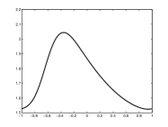 |
 |
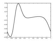 |
| R84 | 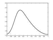 |
 |
 |
| Density | Temperature | Vertical heat flux | |
|---|---|---|---|
| R20 | 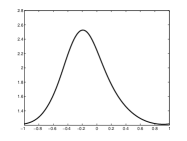 |
 |
 |
| R84 |  |
 |
 |
6 Concluding remarks
A uniform method to solve the regularized moment equations for arbitrary order is proposed. This is the first time that the method for arbitrary order regularized moment equations is developed, and the moment method for large systems is applied to two-dimensional problems. We are now devoting our efforts to the mesh adaptation and parallelization of the algorithm to improve the computational efficiency so that the proposed method can be applied to practical applications.
Acknowledgements
We thank Dr M. Torrilhon for providing us the software for comparison and some useful discussions. The research of the second author was supported in part by a Foundation for the Author of National Excellent Doctoral Dissertation of PRC, the National Basic Research Program of China under the grant 2005CB321701 and the National Science Foundation of China under the grant 10731060.
Appendix
Appendix A Collection of the mathematical symbols
Since lots of mathematical symbols are used in this paper, in order to provide convenience to the readers, we list some of them here.
| The Boltzmann collision operator | |
| The BGK collision operator | |
| The Maxwellian distribution | |
| The basis functions for Grad’s expansion | |
| The Hermite polynomials | |
| The finite dimensional space spanned by , | |
| The discrete distribution function on the cell indexed by at time | |
| The mean velocity and temperature on the cell indexed by at time | |
| The numerical flux between cells indexed by and | |
| The fastest signal velocities travelling in the direction of and | |
| The discrete collision operator | |
| Equivalent to | |
| See (3.21) | |
| The function generated by projecting into | |
| Abbreviation of | |
| The projection operator from to , where and is the mean velocity and temperature of the distribution function | |
| The projection operator from to , where and are the mean velocity and temperature of the distribution function , | |
| A truncation of the distribution (3.1), defined by (4.2) | |
| The th order term in the Chapman-Enskog expansion | |
| The coefficient indexed by in the expansion of the parameter function | |
| The projection operator to the space | |
| Abbreviation of |
Appendix B Calculation of the partial derivative
The calculation of the temporal partial derivative of (3.26) is performed here. Define and as
| (B.1) |
It follows from (3.5) that
| (B.2) |
With the definition of and (3.30), can be related with by
| (B.3) |
Substituting (B.3) into (B.2), and employing the recursion relation of Hermite polynomials, we have
| (B.4) |
where all parameters of , and are omitted. With (B.4), the partial derivative of can be naturally obtained:
| (B.5) |
where
| (B.6) |
Since
| (B.7) |
we finally get
| (B.8) |
where the parameter of , i.e. , is also omitted, and for with negative components, is taken to be zero.
References
- [1] M. Abramowitz and I. A. Stegun. Handbook of Mathematical Functions with Formulas, Graphs, and Mathematical Tables. Dover, New York, 1964.
- [2] J. D. Au, H. Struchtrup, and M. Torrilhon. — an equation generator for extended thermodynamics. Source available on request via M.Torrilhon@vt.tu-berlin.de.
- [3] J. D. Au, M. Torrilhon, and W. Weiss. The shock tube study in extended thermodynamics. Phys. Fluids, 13(8):2423–2432, 2001.
- [4] P. L. Bhatnagar, E. P. Gross, and M. Krook. A model for collision processes in gases. I. small amplitude processes in charged and neutral one-component systems. Phys. Rev., 94(3):511–525, 1954.
- [5] A. V. Bobylev. The Chapman-Enskog and Grad methods for solving the Boltzmann equation. Sov. Phys. Dokl., 27(1):29–31, 1982.
- [6] S. Bochkanov. http://www.alglib.net.
- [7] C. Cercignani, R. Illner, and M. Pulvirenti. The mathematical theory of dilute gases, volume 106 of Applied Mathematical Sciences. Springer, New York, U.S.A., 1994.
- [8] S. Chapman. On the law of distribution of molecular velocities, and on the theory of viscosity and thermal conduction, in a non-uniform simple monatomic gas. Phil. Trans. R. Soc. A, 216(538–548):279–348, 1916.
- [9] P. Degond, L. Pareschi, and G. Russo, editors. Modeling and Computational Methods for Kinetic Equations. Birkhäuser, 2004.
- [10] D. Enskog. The numerical calculation of phenomena in fairly dense gases. Arkiv Mat. Astr. Fys., 16(1):1–60, 1921.
- [11] M. H. Ernst. Nonlinear model — Boltzmann equations and exact solutions. Phys. Rep., 78(1):1–171, 1981.
- [12] H. Grad. On the kinetic theory of rarefied gases. Comm. Pure Appl. Math., 2(4):331–407, 1949.
- [13] H. Grad. The profile of a steady plane shock wave. Comm. Pure Appl. Math., 5(3):257–300, 1952.
- [14] H. Grad. Principles of the kinetic theory of gases. Handbuch der Physik, 12:205–294, 1958.
- [15] X. J. Gu and D. R. Emerson. A computational strategy for the regularized 13 moment equations with enhanced wall-boundary equations. J. Comput. Phys., 255(1):263–283, 2007.
- [16] A. Harten, P. D. Lax, and B. Van Leer. On upstream differencing and Godunov-type schemes for hyperbolic conservation laws. SIAM Review, 25(1):35–61, 1983.
- [17] L. H. Holway. New statistical models for kinetic theory: Methods of construction. Phys. Fluids, 9(1):1658–1673, 1966.
- [18] G. Liu. A method for constructing a model form for the Boltzmann equation. Phys. Fluids A, 2(2):277–280, 1990.
- [19] J. Clerk Maxwell. On stresses in rarified gases arising from inequalities of temperature. Proc. R. Soc. Lond., 27(185–189):304–308, 1878.
- [20] L. Mieussens. Discrete velocity model and implicit scheme for the BGK equation of rarefied gas dynamics. Math. Models Methods Appl. Sci., 10(8):1121–1149, 2000.
- [21] S. Mizzi, X. J. Gu, D. R. Emerson, R. W. Barber, and J. M. Reese. Computational framework for the regularized 20-moment equations for non-equilibrium gas flows. Int. J. Num. Meth. Fluids, 56(8):1433–1439, 2008.
- [22] I. Müller and T. Ruggeri. Rational Extended Thermodynamics, Second Edition, volume 37 of Springer tracts in natural philosophy. Springer-Verlag, New York, 1998.
- [23] E. M. Shakhov. Generalization of the Krook kinetic relaxation equation. Fluid Dyn., 3(5):95–96, 1968.
- [24] X. Shan and X. He. Discretization of the velocity space in the solution of the Boltzmann equation. Phys. Rev. Lett., 80(1):65–68, 1998.
- [25] J. Shen and T. Tang. Spectral and High-Order Methods with Applications, volume 3 of Mathematics Monograph Series. Science Press, Beijing, P. R. China, 2006.
- [26] H. Struchtrup. Macroscopic Transport Equations for Rarefied Gas Flows: Approximation Methods in Kinetic Theory. Springer, 2005.
- [27] H. Struchtrup and M. Torrilhon. Regularization of Grad’s 13 moment equations: Derivation and linear analysis. Phys. Fluids, 15(9):2668–2680, 2003.
- [28] S. Succi. The lattice Boltzmann equation for fluid dynamics and beyond. Oxford University Press, New York, 2001.
- [29] J. Tölke, M. Krafczyk, M. Schulz, and E. Rank. Discretization of the Boltzmann equation in velocity space using a Galerkin approach. Comp. Phys. Comm., 129(1–3):91–99, 2000.
- [30] E. F. Toro. Riemann solvers and numerical methods for fluid dynamics - A practical introduction - 3nd edition. Springer, 2009.
- [31] M. Torrilhon. Characteristic waves and dissipation in the 13-moment-case. Continuum Mech. Thermodyn., 12(5):289–301, 2000.
- [32] M. Torrilhon. Two dimensional bulk microflow simulations based on regularized Grad’s 13-moment equations. SIAM Multiscale Model. Simul., 5(3):695–728, 2006.
- [33] M. Torrilhon, J. Au, D. Reitebuch, and W. Weiss. The Riemann-problem in extended thermodynamics. In H. Freistuühler and G. Warnecke, editors, Hyperbolic Problems: Theory, Numerics, Applications, Vols I and II, volume 140 of International series of numerical mathematics, pages 79–88. Birkhäuser, 2001.
- [34] M. Torrilhon, J. D. Au, and H. Struchtrup. Explicit fluxes and productions for large systems of the moment method based on extended thermodynamics. Cont. Mech. and Ther., 15(1):97–111, 2002.
- [35] M. Torrilhon and R. Jeltsch. Essentially optimal explicit Runge-Kutta methods with application to hyperbolic-parabolic equations. Numer. Math., 106(2):303–334, 2007.
- [36] M. Torrilhon and H. Struchtrup. Regularized 13-moment equations: shock structure calculations and comparison to Burnett models. J. Fluid Mech., 513:171–198, 2004.
- [37] M. Torrilhon and H. Struchtrup. Boundary conditions for regularized 13-moment-equations for micro-channel-flows. J. Comput. Phys., 227(3):1982–2011, 2008.
- [38] M. Torrilhon and H. Struchtrup. Modeling micro mass and heat transfer for gases using extended continuum equations. J. Heat Transfer, 131(3), 2009.
- [39] M. Torrilhon and K. Xu. Stability and consistency of kinetic upwinding for advection-diffusion equations. IMA J. Numer. Analy., 26(4):686–722, 2006.