How to Measure Significance of Community Structure in Complex Networks

Community structure analysis is a powerful tool for complex networks, which can simplify their functional analysis considerably. Recently, many approaches were proposed to community structure detection, but few works were focused on the significance of community structure. Since real networks obtained from complex systems always contain error links, and most of the community detection algorithms have random factors, evaluate the significance of community structure is important and urgent. In this paper, we use the eigenvectors’ stability to characterize the significance of community structures. By employing the eigenvalues of Laplacian matrix of a given network, we can evaluate the significance of its community structure and obtain the optimal number of communities, which are always hard for community detection algorithms. We apply our method to many real networks. We find that significant community structures exist in many social networks and C.elegans neural network, and that less significant community structures appear in protein-interaction networks and metabolic networks. Our method can be applied to broad clustering problems in data mining due to its solid mathematical basis and efficiency.

Complex networks have become a general tool for the analysis of complex systems with many interacting elements. The study of the community structure is of great importance for complex networks (see SantoArxiv as a review). Commonly in many real-world networks, some small subnetworks (communities) have more connections within themselves; but comparatively, they are less likely to be connected with the rest parts. Since nodes in a tight-knit subnetwork have more properties in common, divide the network into such communities could simplify the functional analysis considerably. As a result, the identification of community structure has been the focus of many recent efforts. Generally speaking, such an identification contains two problems: One is to detect the community structure, which was extensively studied during the recent 5 years SantoArxiv ; linear_time ; newman_spectra ; GN ; Systematic ; WLC ; Newman_Q . The second is to evaluate its (community structure) significance, which was hardly settled by researchers in the past. We believe that some networks have clear communities while others don’t. But whether the community structure exists in the network or not, almost all algorithms could find its “community structure”; many algorithms can even find community structures in random networks, which are essentially nonexistent at all. Besides, many real-world networks contain some error links and algorithms of detecting community structure have some random factors Fan . How to evaluate the effects of error links and random factors in the community structure? Therefore, the evaluation of the significance of community structure is imperative. Given a network, it is meaningless to detect the community when the community structure is not significate or when just few error links can considerably change the community structure detected.

In previous works, only a few methods Newman_Q ; Gfeller ; Yhu can evaluate the significance of community structure, and all of them require to know the community structure before the evaluation. However, the significance of community structure should be the property of network itself, which is independent of the partition algorithm, and can be evaluated without knowing the exact communities. According to the well studied bi-communities of network Newman_Q , to calculate the significance of community structure can be transformed to measure the stability of eigenvectors. In the following sections, we will extend the bi-communities problem to multi-communities problem and design an index to evaluate the significance of the community structure. Furthermore, we apply the method to many types of networks. We find that C. elegans neural network and social networks usually have distinct community structure, while metabolic networks and protein-interaction networks don’t. The results are consistent with our previous research Yhu .

I Method

How to evaluate the impact of error links and random factors of algorithm? The two aspects can be merged into one problem. We can regard the random factors of algorithms as error link liked cases. That is, we can suggest that all random factors are caused by error links. If the community structure is very clear, a few error links will not impact the structure greatly, neither will the random factors of algorithm Fan . Otherwise, if the community structure is fuzzy, few error links will affect the structure greatly and the random factors of algorithm will also induce a big change in community structure. So, the only problem is how to evaluate the effect of error links for community structure. We will propose a method to evaluate the significance. The method admits solid mathematical basis, so that the analysis of significance is easy and reliable. Hence, the significance of community structure can be evaluated effectively.

I.1 Robustness of Community Structure

We begin by defining the adjacency matrix A of a network, which consists of elements: $A_{i,j}=1$ when there is an edge joining vertices $i$ and $j$; 0 otherwise. The corresponding Laplacian matrix L is defined as: $L_{i,j}=-A_{i,j}$ if $i\neq j$, and $L_{i,i}=k_{i}$, where $k_{i}$ is the degree of node $i$. $\lambda_{i}$ is the eigenvalue and $\textbf{v}_{i}$ is the corresponding eigenvector of L. Moreover, we let $0=\lambda_{1}\leq\lambda_{2}\leq\lambda_{3}\leq\cdots\leq\lambda_{n}$, $\textbf{v}_{i}^{T}\textbf{v}_{j}=0$ if $i\neq j$, and $\textbf{v}_{i}^{T}\textbf{v}_{i}=1$ for all $i$. In the well studied bi-community problem newman_spectra (partition the network into two communities with pre-knowledge the size of each community), the community structure vector s with elements $s_{i}$ is defined as: $s_{i}=1$ if node $i$ belongs to community $1$ and $s_{i}=-1$ if node $i$ belongs to community $2$. s can be written as a linear combination of the normalized eigenvectors $\textbf{v}_{i}$. Thus, $\textbf{s}=\sum_{i=1}^{n}a_{i}\textbf{v}_{i}$, where $a_{i}=\textbf{v}_{i}^{T}\textbf{s}$. Since $\textbf{s}^{T}\textbf{s}=n$, $\sum{a_{i}^{2}}=n$, the bi-community problem can be written as an optimization problem:

$$MinZ=\textbf{s}^{T}\textbf{L}\textbf{s}=\sum{a_{i}^{2}\lambda_{i}}.$$ (1)

where $\frac{1}{4}Z$ is the number of links between the two partitioned communities.

To minimize $Z$ is always a tough problem and can be equated with the task of choosing the nonnegative quantities $a_{i}^{2}$ so as to place as much as possible of the weight in the sum in the terms corresponding to the lowest eigenvalues and as little as possible in the terms corresponding to the highest eigenvalues newman_spectra . So the above optimization problem can be simplified as:

$$MinZ\approx Max\hat{Z}=a_{2}^{2}\lambda_{2}$$ (2)

Now we will extend the above bi-community network problem to multi-community network one. Suppose that a network has $n$ nodes and $c$ communities, and we have $0=\lambda_{1}\leq\lambda_{2}\approx\lambda_{3}\approx\cdots\approx\lambda_{c}\leq\lambda_{c+1}\leq\cdots\leq\lambda_{n}$ Systematic . $\textbf{S}_{1}$ denotes the community vector of community one. If node $i$ belongs to community one, $S_{1,i}=1$ and $-1$ otherwise. Then $\frac{1}{4}\textbf{S}_{1}^{T}\textbf{L}\textbf{S}_{1}$ is the number of edges between community 1 and the rest of the network. Consequently, we can define quantitatively the optimal partition as:

$$MinZ=\sum_{i=1}^{c}\textbf{S}_{i}^{T}\textbf{L}\textbf{S}_{i}.$$ (3)

Let $\textbf{S}=(\textbf{S}_{1}^{T},\textbf{S}_{2}^{T},\cdots,\textbf{S}_{c}^{T})^{T}$ and $\hat{\textbf{L}}=diag(\textbf{L},\textbf{L},\cdots,\textbf{L})$, thus, we have

$$MinZ=\textbf{S}^{T}\hat{\textbf{L}}\textbf{S}.$$ (4)

We can obtain all orthogonal and normalized eigenvectors $\textbf{u}_{q}$ and the corresponding eigenvalues $\tau_{q}$ of $\hat{\textbf{L}}$, where $q=1,2,\cdots,n\times c$. Obviously, each eigenvalue of L is $\hat{\textbf{L}}$’s eigenvalue and repeat $c$ times. Without loss of generality, we let $\tau_{ci-c+j}=\lambda_{i},j=1,2,\cdots,c$. Let SU be the eigenvectors set of the eigenvalues of $\lambda_{2},\lambda_{3},\cdots,\lambda_{c}$ of matrix $\hat{\textbf{L}}$. SU can be written as $\textbf{SU}=\{(\textbf{v}_{2}^{T},0\cdots,0),\cdots,(\textbf{v}_{c}^{T},0,\cdots,0),\cdots,(0,0,\cdots,\textbf{v}_{c}^{T})\}$, where each $0$ denote an $n$-dimensional zero vector and SU has $c\times(c-1)$ elements. We can expand SU as a space SSU in which each point is the liner combination of the elements in set SU. The multi-partition problem can be written as:

$$MinZ=\sum_{q=1}^{n\times c}b_{q}^{2}\tau_{q}\approx Max\hat{Z}=\sum_{\textbf{u}_{q}\in\textbf{SSU}}b_{q}^{2}\tau_{q}\approx\bar{\lambda}\sum_{\textbf{u}_{q}\in\textbf{SSU}}b_{q}^{2}$$ (5)

where $b_{q}=\textbf{S}^{T}\textbf{u}_{q}$ and $\bar{\lambda}$ is the average value of $\tau_{c+1}$ to $\tau_{c\times c}$ (also is the average value of $\lambda_{2}$ to $\lambda_{c}$). $\sum_{\textbf{u}_{q}\in\textbf{SSU}}b_{q}^{2}$ denotes the length of vector S projection in space SSU. Obviously, the longer the projection is, the nearer S approaches the optimal. It is difficult to obtain the optimal S. In this paper, we focus on how to evaluate the significance of community structure. Could we avoid the tough problem and measure the community structure significance? For a network with a clear community structure, even if there are a few error links the community structure should be change a little. In contrast, when its community structure is fuzzy, a few error links or a slight perturbation will lead to a big change in the community structure. This property should be reflected in space SSU. That is, for the same change of links, if the community structure is significant, the space SSU will change a little; otherwise it will change considerably. The space SSU is expanded by the simple combination of $\textbf{v}_{2},\textbf{v}_{3},\cdots,\textbf{v}_{c}$; therefore, the robustness of space SSU equals the robustness of the eigenvalues $\lambda_{2},\lambda_{3},\cdots,\lambda_{c}$ and eigenvectors $\textbf{v}_{2},\textbf{v}_{3},\cdots,\textbf{v}_{c}$.

Suppose that, $\delta A$ is the perturbation links for the original network. Then, we can write $\delta L,\,\,\delta\lambda_{i}$ and $\delta v_{i}$ as the corresponding perturbation of the Laplacian matrix $L$ and its eigenvalues and eigenvectors. According to the eigenvalue and eigenvector stability theory Russia , we have the following equations:

$$(\delta\textbf{L}+\textbf{L})(\delta\textbf{v}_{i}+\textbf{v}_{i})=(\delta\lambda_{i}+\lambda_{i})(\delta\textbf{v}_{i}+\textbf{v}_{i})$$ (6)

by deleting the second-order small quantities, we have

$$\delta\textbf{L}\textbf{v}_{i}+\textbf{L}\delta\textbf{v}_{i}=\lambda_{i}\delta\textbf{v}_{i}+\delta\lambda_{i}\textbf{v}_{i}$$ (7)

after some deductions we obtain:

$$\delta\lambda_{i}=\frac{\textbf{v}_{i}^{T}\delta\textbf{L}\textbf{v}_{i}}{\textbf{v}_{i}^{T}\textbf{v}_{i}},\,\,\,\,\delta\textbf{v}_{i}=\sum_{j=1}^{n}h_{ij}\textbf{v}_{j}$$ (8)

where, $h_{ij}=\frac{\textbf{v}_{j}^{T}\delta\textbf{L}\textbf{v}_{i}}{\textbf{v}_{j}^{T}\textbf{v}_{j}(\lambda_{i}-\lambda_{j})},(i\neq j).$ Therefore, we have

$$|\delta\lambda_{i}|\leq\|\delta\textbf{L}\|$$ (9)

which implies that for any network, no matter the community structure is significant or not, the eigenvalues are only related to the perturbation strength. In this way, the eigenvalues are always stable Russia . (So, it is not necessary to consider the stability of eigenvalues.)

Without loss of generality, we can let $a_{i1}=a_{ii}=0$ for $i\neq 1$. Then the comparative error of $v_{i}$ can be denoted as

$$\frac{|\delta\textbf{v}_{i}|}{|\textbf{v}_{i}|}\leq\parallel\delta\textbf{L}\parallel\sum_{j\neq i,j=2}^{n}\frac{1}{|\lambda_{i}-\lambda_{j}|}$$ (10)

In Eq.10, $\parallel\delta L\parallel$ is the perturbation strength and $\sum_{j\neq i,j=2}^{n}\frac{1}{|\lambda_{i}-\lambda_{j}|}$ is the amplification coefficient which is used to measure the stability of $\textbf{v}_{i}$. Integrating the stability of $\lambda_{2}$ to $\lambda_{c}$, we define $R$ as the stability index of space SSU.

$$R=\sum_{j=c+1}^{n}\frac{1}{|\bar{\lambda}-\lambda_{j}|}$$ (11)

Of cause, $R$ is an important index of the network which can be used to measure the significance of community structure.

I.2 Index of the Significance

Although $R$ makes sense mathematically, it is not convenient to measure and further compare the significance of different networks. In this section, we will define an efficient index to measure the community structure significance. Like the definition of temperature, if we know the most significant and fuzzy stability values $R$, the robustness can be scaled into interval $[0,1]$ which will be very intuitive to use.

What kind of network possess the most significant community structure? Suppose that the network size is $n$, the average degree is $k$ and the community number is $c$, where $c<<n$. To find the most significant community structure is to solve the following optimization problem:

$$\left\{\begin{aligned} MinR=\sum_{i=c+1}^{n}\frac{1}{\lambda_{c+1}-\bar{\lambda}}\\ s.t.\ \ \ \ \ \ \ \ \ \ \sum_{i=1}^{n}\lambda_{i}=nk.\end{aligned}\right.$$ (12)

For the above optimization problem, we directly set $\bar{\lambda}=0$. By the Lagrange multiplier method, we obtain that when $\bar{\lambda}=0,\lambda_{c+1},\lambda_{c+2},\cdots,\lambda_{n}=\frac{nk}{n-c}$, $R$ will achieve it’s global minimum value $R=\frac{(n-c)^{2}}{nk}\approx\frac{n}{k}$. $\bar{\lambda}=0$ implies that there are no any connections among communities and the network is not connected which is not suitable for our basic assumption. But this kind of unconnected network can be modified slightly to meet our requirement. We can generate a network with $c=\frac{n}{k+1}$ communities, and each community, which is a completely connected subgraph, contains $k+1$ nodes. Among the $c$ communities there are only $c-1$, connections which guarantee that the whole network is connected. For this kind of network, $\bar{\lambda}\approx 0,\lambda_{c+1},\lambda_{c+2},\cdots,\lambda_{n}\approx k+1$, and the corresponding $R$ will achieve the global minimum value $R\approx\frac{n}{k}$, as shown in Fig. 1 a.

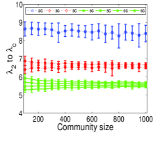
Figure 1: a. The dependence of maximum $h$ and community number on artificial connected networks. Given a degree $k$, each community is a completely connected subgraph with $k+1$ nodes. Among the communities there are $c-1$ connections making the whole network connected, where $c$ is the number of communities. From the plot we can see that the maximum $h$ is very close to 1. b. The dependence of $\lambda_{2}$ to $\lambda_{c}$ and community size. In this plot, $2C,3C,5C$ denote that there are 2,3 and 5 equal communities in the network respectively. Each node has 20 expected links with its fellows with the same community and 5 expected links with other communities. The error bar denotes the standard deviation. We can see that the standard deviation of $\lambda_{2}$ to $\lambda_{c}$ is small and it does not depend on the size of community considerably.

The spectra properties of complex network matrix have been well studied Num_spec ; Laplacian_spectra . They throw a light on the universal properties of the eigenvalues’ distribution of random spares matrices. We investigate the distribution of eigenvalues for different community structures in both homogeneous (passion) and heterogeneous (scale free) degree distribution networks. The results show that the distribution of eigenvalues is mainly determined by the average degree and degree distribution, and does not relate to the community structure considerably (as shown in Fig. 2). Moreover, for networks with different size and community structure, we investigate the most relavent eigenvalues $\lambda_{2},\lambda_{3},\cdots,\lambda_{c}$, and we also find that they, staying, depend only on the community structure and does not related to the size of both community and network (as shown in Fig. 1 b).

According to Num_spec ; Laplacian_spectra , Eq. 11 and Fig.2, we have $R\propto n$ strictly as shown in Fig. 3. From Fig. 3 we can see that, for both homogeneous and heterogeneous degree distribution, the great mass of eigenvalues $\lambda$ are near the average degree, although the distribution of eigenvalues can not be scaled by the average degree. We have conducted many numerical experiments in both homogeneous and heterogeneous networks and find that $\frac{1}{R}\propto k$ holds well. Therefor, given a network with robustness $R=h\frac{n}{k}$, when the community structure is more significant, $h$ will be small. From the above analysis of the clearest community structure in a large enough network, we have a lower bound, which almost approaches $1$. It is very hard to get the $h$ of a fuzziest community structure for that the continuous property of matrix spectra is very complicated. So, to simplify the index, we define $H=\frac{1}{h}=\frac{n}{Rk}$ as the significance of community structure and $H$ is almost in $[0,1]$ when network size is large enough.

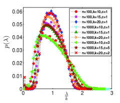
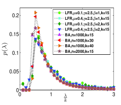
Figure 2: The distribution of laplace matrix’s eigenvalues. Community structure has no considerable impact on its eigenvalue’s distribution for both homogeneous and heterogeneous networks. The eigenvalues’ distribution can be scaled by average degree for both homogeneous and heterogeneous networks. The relative width of this peak decreases with increasing average degree, while other qualitative features are the same.a. In homogeneous networks, each community is a ER network. The legend $c=1$ means that the network is a ER network without communities. When $c=2$, the two communities size is $100$ and $900$ respectively. When $c=3$, there are 3 communities and the communities size is $100,200,700$. $c=5$, all the community sizes are 200. We also test many other community size distribution and the results are same (not yet been shown here). b. We employ the LFR-benchmark and the BA model to generate the heterogeneous network. In the LFR-benchmark, we set the maximum degree as $50$, and the maximum and minimum community sizes is $50$ and $20$ respectively.

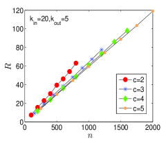
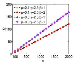
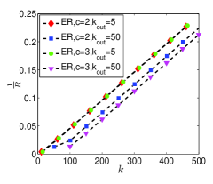
a       b
c       d

Figure 3: The relationship of $R\propto\frac{n}{k}$. From the four plots we can see that $R\propto\frac{n}{k}$ is almost validate. a. The dependence of $R$ on the network size $n$. Each community size is the same and each node has 20 links to others in the same community and 5 links to the outside nodes. $c$ is the community number. b. The dependence of $R$ and network size $n$ in the LFR benchmark. The average degree $k=20$ and $P(k)\propto k^{2.5}$, the maximum degree is $50$, maximum and minimum community size is $20,50$ respectively. c. The dependence of $\frac{1}{R}$ and average degree $k$. For different network size $n$, each community size are same. d. The dependence of $\frac{1}{R}$ and average degree $k$ in the LFR benchmark.The maximum degree is $200$ and maximum and minimum community size is $200,100$ respectively. Average degree is 20 and $P(k)\propto k^{2.5}$.

II Result

II.1 Artificial Networks

Let’s test the validity of our index. Firstly, we use the classical GN benchmark presented by Girvens and Newman Newman_Q . Each network has $n=128$ nodes that are divided into $4$ communities with $32$ nodes each. Edges between two nodes are introduced with different probabilities which depend on whether the two nodes belong to the same community or not. Each node has $\langle k_{in}\rangle$ links on average with its fellows in the same community, and $\langle k_{out}\rangle$ links with the other communities, and we keep $\langle k_{in}\rangle+\langle k_{out}\rangle=16$. As is well known, the communities become fuzzier and thus more difficult to be identified when $k_{out}$ increases. Hence, the significance of the community structure will also tend to be weaker and the $R$ index will decrease. The numerical experiments’ results are shown in Fig. 4. We can find that the index $H$ works well in the GN-benchmark. When community structure is very clear, the $H$ is very close to $1$; when the network is nearly a random one, the corresponding $H$ is near to $0.3$. Thus, we argue that for a given network when the corresponding $H$ is larger than 0.3, there exists community structure. Moreover, the larger the $H$ index is, the more significant community structure will be.

We also test the index on the more challenging LRF benchmark presented by Lancichinetti, Fortunato, Radicchi LFR . In the LFR benchmark, each node is given a degree took from a power law distribution with an exponent $\gamma$, and the sizes of the communities are took from a power law distribution with an exponent $\beta$. Moreover, each node shares a fraction $1-\mu$ of its links with other nodes of its community and a fraction $\mu$ with other nodes in the network. $\mu$ is the mixing parameter. The community structure significance can be adjusted by the mixing parameter $\mu$. The numerical results in the LFR-benchmark are shown in Fig. 4. We can see that $H$ decreases with the augment of $\mu$ and $H$ is independent of the community size distribution. Moreover, when the power law exponent of degree distribution becomes larger, the community structure will be more significant. That more homogenous the degree distribution is, the more significant the community structure will be, when other conditions are same.

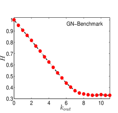
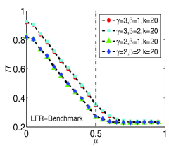
Figure 4: The performance of $H$ index in both GN-benchmark and LFR-benchmark. In GN-benchmark, we can see that $H$ decrease with increasing of $k_{out}$. When the community structure is very clear $H$ close to 1 very much, and the network close to no community structure network $H$ close to 0.3 which implies that for a given network when $H$ is less than 0.3 it is not safe to say there exit significant community structure. In LFR-benchmark, the average degree $k=20$, maximum degree is $50$ and $P(k)\propto k^{\gamma}.$ Maximum and minimum community sizes are $50$ and $20$ respectively, more over $Q(m)\propto m^{\beta}$ where, $m$ denotes the community size. We can see that with the increase of mix parameter $\mu$, the $H$ index decrease. When $\mu\geq 0.5$ (no significant community) $H$ is near $0.3$ which is similar with GN-benchmark.

II.2 Real-world Networks

Till now, we still haven’t discuss how to obtain the optimal community number $c$. For many real-world networks, we don’t know the community number before calculating the index value or partition. Many numerical experiments (as shown in Fig. 5) support that the community structure will be most clearest when the community number is the optimal $c$. So generally speaking, the corresponding community number with the lowest $R$ will be the optimal $c$. Moreover, at the optimal $c$, the value of $\lambda_{c+1}-\lambda_{c}$ will be very large comparatively. So we also can resort to the differences between $\lambda_{i}$ and $\lambda_{i+1}$ to detect the optimal $c$.

We apply the index to many real networks (see Tab.1 and detail information in supplementary). The data are taken from the following references and web sites ZK_d ; Dolphin ; Ploblog ; C.neural ; Jazz ; C.met ; webset1 ; webset2 ; webset3 . People usually classify the real networks into three categories: social networks (such as scientist collaborations and friendships), biological networks (such as proteins interaction networks and metabolic networks) and technological networks (such as Internet and the WWW). First, we analyze several social networks, including Zachary karate club network ZK_d , dolphin network Dolphin , collage football network GN , Jazz network Jazz , scientists collaboration network webset1 and so on. The results are very similar to our previous work Yhu . We find that the Jazz community structure is the most significant one, the Santa Fe scientists collaboration network and the Political blogs network are insignificant comparatively. Generally speaking, the community structure is most notable in social networks. Moreover, we analyze some biological networks such as proteins interaction networks (E. coli webset2 , Yeast webset3 and H. Sapiens webset2 ), many metabolic networks webset3 and C.elegans neural network. We find that in proteins interaction networks, E.coli is 0.14, H. Sapiens 0.21, and Yeast 0.40, which is high and different from the previous results. In metabolic networks, the $H$ index of Aquifex aeolicus, Helicobacter pylori and Yersinia pestis are all 0.36, which are consistent to previous works. But for the C.elegans metabolic and neural network , significance is 0.62, which is very high and different from previous work due to it is not easy to obtain the proper community number $c$ (see supplementary). The significance of C.elegans neural is 0.57, which corresponds to previous work well.

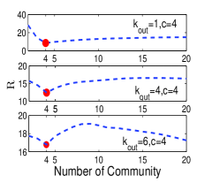
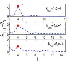
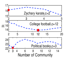
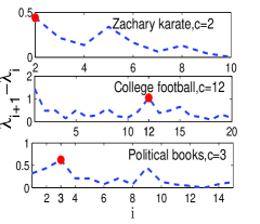
a       b
c       d

Figure 5: The optimal community number. The rang optimal $c$ is about $\frac{n}{10}$ for all networks. From the plots a and b we can find that on GN-benchmark, when $c=4$ (pre-determined community number) $R$ achive lowest value and the corresponding $\lambda_{c+1}-\lambda_{c}$ also achieve the largest value. c and d The empirical results of Zachary karate club network, College football network and Political books network. It was found that Zachary karate club has 2 communities and College football network has 12 communities. Form the plots we can see that $R$ achieve its lowest value when the community numbers correspond the reality. The corresponding values of $\lambda_{i+1}-\lambda_{i}$ also present reasonable phenomenons. For the Political books, we still don’t know how many communities, the method shows that it has 3 communities.

Table 1: The $\hat{R}$ and $H$ indexes of some real networks. $\hat{R}$ indexes is the robustness of community structure, which can be obtain be perturbation (please see ref Yhu ). The table shows the names of different real networks and the corresponding index values.

network	size	$\hat{S}$	$\hat{R}$	H	type
E.coli	1442, 5873	61.30	0.11	0.14
Yeast	1458, 1971	112.95	0.12	0.40	protein
H.Sapiens	693, 982	38.48	0.18	0.21
C.elegans metabolic	453, 2032	19.25	0.17	0.62
Aquifex aeolicus	1473, 3354	68.39	0.17	0.36
Helicobacter pylori	1341, 3087	62.76	0.17	0.36	metabolic
Yersinia pestis	1922, 4389	108.84	0.15	0.36
43 metabolic networks	1472, 3395	71.25	0.17	0.36
C.elegans neural	297, 2148	5.52	0.22	0.52	neural
Santa Fe scientists	118, 200	2.45	0.27	0.72
Zachary karate	34, 78	0.32	0.25	0.46
Dolphin	62, 159	2.07	0.24	0.42
College football	115, 613	1.67	0.34	0.79	social
Jazz	198, 2742	0.64	0.40	0.47
Email	1133,5452	27.35	0.19	0.42
Political blogs	1222, 19090	0.57	0.27	0.22
Political books	105, 441	1.63	0.31	0.32

III Conclusion and discussion

In this paper, an index to evaluate the significance of community structure without knowing the community structure is proposed. We transform the problem of community structure significance into the problem of the stability of eigenvalues and eigenvectors of the Laplacian matrix. The index of community structure significance admits sound mathematical basis, which makes the index is reliable. According to the index, the optimal community number can also be obtained before partition, which is nearly impossible for many partition algorithms. Moreover, we apply the index to many real world networks, such as social networks, neural network, protein-interaction networks and metabolic networks. We find that in social networks, the significance of community structure is usually high, C.elegans metabolic and neural networks they are very hight, and in protein interaction and some other metabolical, they are comparative low.

IV Supplementary

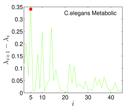
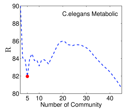
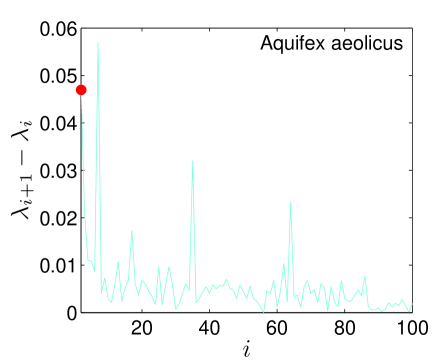
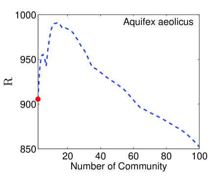
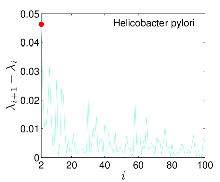
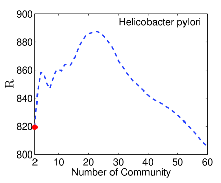
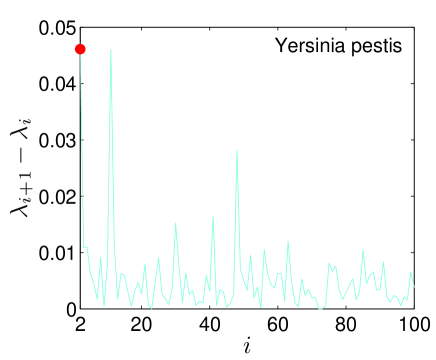
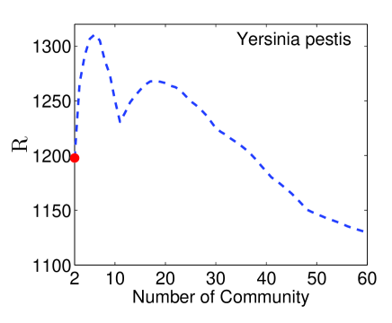
Figure 6:

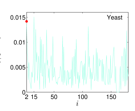
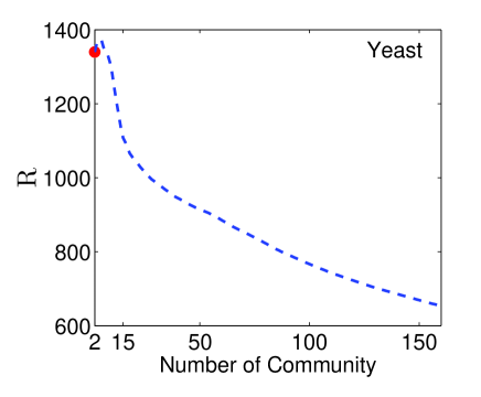
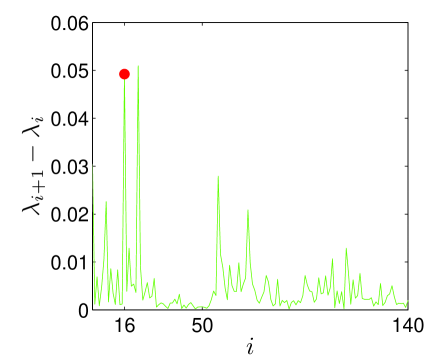
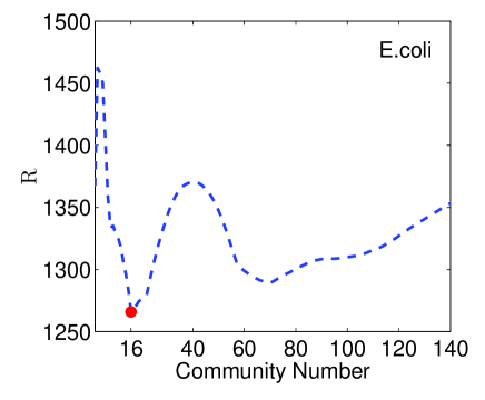
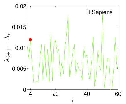
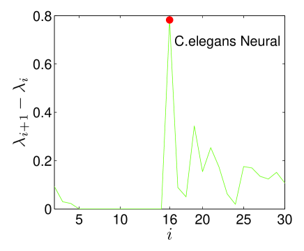
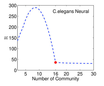
Figure 7:

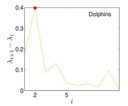
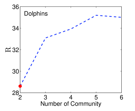
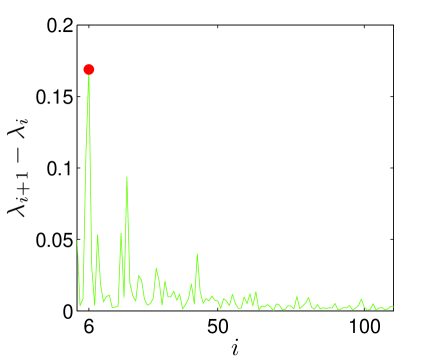
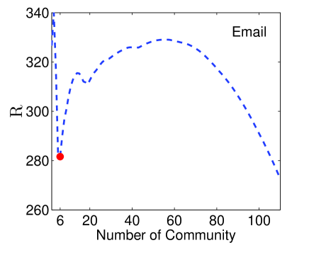
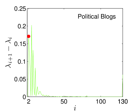
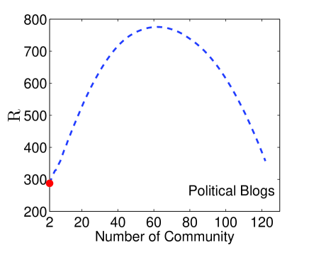
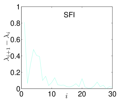
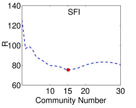
Figure 8:

References

- (1) S. Fortunato, arXiv:0906.0612v1, (2009).
- (2) Wu, F. and Huberman, B. A. (2004) Finding communities in linear time: a physics approach. Eur. Phys. J. B. 38:331-338.
- (3) Newman, M. E. J. (2006) Finding community structure in networks using the eigenvectors of matrices. Phys. Rev. E. 74: 036104.
- (4) Girvan, M. and Newman, M. E. J. (2002) Community structure in social and biological networks. Proc. Natl. Acad. 99: 7821-7826.
- (5) Donetti, L. and Munoz, M. A. (2004) Detecting network communities: a new systematic and efficient algorithm. J. Stat. Mech. P10012.
- (6) Wang, X., Li, X. and Cheng, G. (2006) Complex network thory and application. Tsinghua University Press. Page 162-193.
- (7) Newman, M. E. J. (2006) Modularity and community structure in networks. Proc. Natl. Acad. 103: 8577-8582
- (8) Fan, Y., Li, M., Zhang, P., Wu, J. and Di, Z. (2007) Accuracy and precision of methods for community identification in weighted networks. Physica A 377: 363-372 .
- (9) G. Bianconi, G., Pin, P. and Marsili, M. (2009) Assessing the relevance of node features for network structure. Proc. Natl. Acad. 106: 11433-11438.
- (10) Gfeller, D., Chappelier, J.-C. and de Los Rios, P. (2005) Finding instabilities in the community strucuture of complex networks. Phys. Rev. E 72: 056135.
- (11) Hu, Y., Nie, Y., Yang, Y., Cheng, J., Fan, Y. and Di, Z. Measuring Significance of Community Structure in Complex Networks. arXiv:0906.0493, (2009)
- (12) McGraw, P. N. and Menzinger, M. (2008) Laplacian spectra as a diagnostic tool for network structure and dynamics. Phys. Rev. E. 77: 031102.
- (13) Dorogovtsev, S. N., Goltsev, A. V., Mendes, J. F. and Samukhin, A. N. (2003) Spectra of complex networks. Phys. Rev. E 68: 046109.
- (14) Faddeev I, D. K., FaDDeeva, V. N. (1965) Calculation method of linear algebra. Shanghai Science and Technology Press (Translated into Chinese by Li, G. et al).
- (15) Lancichinetti, A., Fortunato, F. and Radicchi, F. (2008) Benchmark graphs for testing community detection algorithms. Phys. Rev. E. 78: 046110.
- (16) Zachary, W. W. Journal of Anthropological Research 33: 452-473 (1977).
- (17) Lusseau, D., Schneider, K., Boisseau, O. J., Haase, P., Slooten, E. and Dawson, S. M. (2003) The bottlenose dolphin community of Doubtful Sound features a large proportion of long-lasting associations. Behavioral Ecology and Sociobiology 54: 396-405.
- (18) Adamic, L. A. and Glance, N. (2005) The Political Blogosphere and the 2004 U.S. Election: Divided They Blog. The political blogosphere and the 2004 US Election, in Proceedings of the WWW-2005 Workshop on the Weblogging Ecosystem.
- (19) Watts, D. J. and Strogatz, S. H. (1998) Collective dynamics of ’small-world’networks. Nature 393: 440-442.
- (20) Gleiser, P. and L. Danon, L. (2003) Community structure in jazz. Adv. Complex Syst. 6: 565.
- (21) J. Duch and A. Arenas, Phys. Rev. E. 72: 027104, (2005).
- (22) http://www-personal.umich.edu/ mejn/netdata/
- (23) Database of Interacting Proteins (DIP). http://dip.doe-mbi.ucla.edu
- (24) http://www.nd.edu/ networks