1. Introduction

This paper presents a numerical technique for solving boundary integral equations (BIEs) defined on axisymmetric surfaces in $\mathbb{R}^{3}$. Specifically, we consider second kind Fredholm equations of the form

(1.1) $$\sigma({\boldsymbol{x}})+\int_{\Gamma}k(\boldsymbol{x},\boldsymbol{x}^{\prime})\,\sigma(\boldsymbol{x}^{\prime})\,dA(\boldsymbol{x}^{\prime})=f(\boldsymbol{x}),\hskip 10.00002pt\boldsymbol{x}\in\Gamma,$$

under two assumptions: First, that $\Gamma$ is a surface in $\mathbb{R}^{3}$ obtained by rotating a curve $\gamma$ about an axis. Second, that the kernel $k$ is invariant under rotation about the symmetry axis in the sense that

(1.2) $$k(\boldsymbol{x},\boldsymbol{x}^{\prime})=k(\theta-\theta^{\prime},r,z,r^{\prime},z^{\prime}),$$

where $(r,\,z,\,\theta)$ and $(r^{\prime},\,z^{\prime},\,\theta^{\prime})$ are cylindrical coordinates for $\boldsymbol{x}$ and $\boldsymbol{x}^{\prime}$, respectively,

$$\boldsymbol{x} =(r\,\cos\theta,\,r\,\sin\theta,\,z),$$

$$\boldsymbol{x}^{\prime} =(r^{\prime}\,\cos\theta^{\prime},\,r^{\prime}\,\sin\theta^{\prime},\,z^{\prime}),$$

see Figure 1.1. Under these assumptions, the equation (1.1), which is defined on the two-dimensional surface $\Gamma$, can via a Fourier transform in the azimuthal variable be recast as a sequence of equations defined on the one-dimensional curve $\gamma$. To be precise, letting $\sigma_{n}$, $f_{n}$, and $k_{n}$ denote the Fourier coefficients of $\sigma$, $f$, and $k$, respectively (so that (2.6), (2.7), and (2.8) hold), the equation (1.1) is equivalent to the sequence of equations

(1.3) $$\sigma_{n}(r,z)+\sqrt{2\pi}\int_{\gamma}k_{n}(r,z,r^{\prime},z^{\prime})\,\sigma_{n}(r^{\prime},z^{\prime})\,r^{\prime}\,dl(r^{\prime},z^{\prime})=f_{n}(r,z),\hskip 10.00002pt(r,z)\in\gamma,\hskip 5.0ptn\in\mathbb{Z}.$$

Whenever $f$ can be represented with a moderate number of Fourier modes, the formula (1.3) provides an efficient technique for computing the corresponding modes of $\sigma$. The conversion of (1.1) to (1.3) appears in, e.g., [Rizzo:79a], and is described in detail in Section 2.

Equations of the type (1.1) arise in many areas of mathematical physics and engineering, commonly as reformulations of elliptic partial differential equations. Advantages of a BIE approach include a reduction in dimensionality, often a radical improvement in the conditioning of the mathematical equation to be solved, a natural way of handling problems defined on exterior domains, and a relative ease in implementing high-order discretization schemes, see, e.g., [Atkinson:97a].

The numerical solution of BIEs such as (1.1) poses certain difficulties, the foremost being that the discretizations generally involve dense matrices. Until the 1980s, this issue often times made it prohibitively expensive to use BIE formulations as numerical tools. However, with the advent of “fast” algorithms (the Fast Multipole Method [rokhlin1987, rokhlin1997], panel clustering [hackbusch_1987], etc.) for matrix-vector multiplication and the inversion of dense matrices arising from the discretization of BIE operators, these problems have largely been overcome for problems in two dimensions. This is not necessarily the case in three dimensions; issues such as surface representation and the construction of quadrature rules in a three dimensional environment still pose unresolved questions. The point of recasting the single BIE (1.1) defined on a surface as the sequence of BIEs (1.3) defined on a curve is in part to avoid these difficulties in discretizing surfaces, and in part to exploit the exceptionally high speed of the Fast Fourier Transform (FFT).

The reduction of (1.1) to (1.3) is only applicable when the geometry of the boundary is axisymmetric, but presents no such restriction in regard to the boundary load. Formulations of this kind have been known for a long time, and have been applied to problems in stress analysis [Bakr:85a], scattering [Fleming:04a, Kuijpers:97a, Soenarko:93a, Tsinopoulos:99a, Wang:97a], and potential theory [Gupta:1979a, Provatidis:98a, Rizzo:79a, Shippy:80a]. Most of these approaches have relied on collocation or Galerkin discretizations and have generally relied on low-order accurate discretizations. A complication of the axisymmetric formulation is the need to determine the kernels $k_{n}$ for a large number of Fourier modes $n$, since direct integration of (1.2) through the azimuthal variable tends to be prohibitively expensive. When $k$ is smooth, this calculation can rapidly be accomplished using the FFT, but when $k$ is near-singular, other techniques are required (quadrature, local refinement, etc.) that can lead to significant slowdown in the construction of the linear systems.

The technique described in this paper improves upon previous work in terms of both accuracy and speed. The gain in accuracy is attained by constructing a high-order quadrature scheme for kernels with integrable singularities. This quadrature is obtained by locally modifying a Guassian quadrature scheme, in a manner similar to that of [Bremer:a, Bremer:b]. Numerical experiments indicate that for simple surfaces, a relative accuracy of $10^{-10}$ is obtained using as few as a hundred points along the generating curve. The rapid convergence of the discretization leads to linear systems of small size that can be solved directly via, e.g., Gaussian elimination, making the algorithm particularly effective in environments involving multiple right hand sides and when the linear system is ill-conditioned. To describe the asymptotic complexity of the method, we need to introduce some notation. We let $N_{\rm P}$ denote the number of panels used to discretize the generating curve $\gamma$, we let $N_{\rm G}$ denote the number of Gaussian points in each panel, and we let $N_{\rm F}$ denote the number of Fourier modes included in the calculation. Splitting the computational cost into a “set-up” cost that needs to be incurred only once for a given geometry and given discretization parameters, and a “solve” cost representing the time required to process each right hand side, we have

(1.4) $$T_{\rm setup}\sim\underbrace{N_{\rm P}^{2}\,N_{\rm G}^{2}\,N_{\rm F}\,\log(N_{\rm F})+N_{\rm P}\,N_{\rm G}^{3}\,N_{\rm F}^{2}}_{\textrm{construction of linear systems}}\hskip 11.99998pt+\underbrace{N_{\rm P}^{3}\,N_{\rm G}^{3}\,N_{\rm F}}_{\textrm{inversion of systems}},$$

and

(1.5) $$T_{\rm solve}\sim\underbrace{N_{\rm P}\,N_{\rm G}\,N_{\rm F}\,\log(N_{\rm F})}_{\textrm{FFT of boundary data}}\hskip 12.50002pt+\underbrace{N_{\rm P}^{2}\,N_{\rm G}^{2}\,N_{\rm F}}_{\textrm{application of inverses}}.$$

The technique described gets particularly efficient for problems of the form (1.1) in which the kernel $k$ is either the single or the double layer potential associated with Laplace’s equation. We demonstrate that for such problems, it is possible to exploit recursion relations for Legendre functions to very rapidly construct the Fourier coefficients $k_{n}$ in (1.3). This reduces the computational complexity of the setup (which requires the construction of a sequence of dense matrices) from (1.4) to

$$T_{\rm setup}\sim N_{\rm P}^{2}\,N_{\rm G}^{2}\,N_{\rm F}\,\log(N_{\rm F})+N_{\rm P}\,N_{\rm G}^{3}\,N_{\rm F}+N_{\rm P}^{3}\,N_{\rm G}^{3}\,N_{\rm F}.$$

Numerical experiments demonstrate that for a problem with $N_{\rm{P}}=80$, $N_{\rm{G}}=10$, and $N_{\rm F}=400$ (for a total of $80\times 10\times 400=320\,000$ degrees of freedom), this accelerated scheme requires only 2.2 minutes for the setup, and 0.46 seconds for each solve when implemented on a standard desktop PC.

The technique described in this paper can be accelerated further by combining it with a fast solver applied to each of the equations in (1.3), such as those based on the Fast Multipole Method, or the fast direct solver of [Martinsson:04a]. This would result in a highly accurate scheme with near optimal complexity.

The paper is organized as follows: Section 2 describes the reduction of (1.1) to (1.3) and quantifies the error incurred by truncating the Fourier series. Section 3 presents the Nyström discretization of the reduced equations using high-order quadrature applicable to kernels with integrable singularities, and the construction of the resulting linear systems. Section 4 summarizes the algorithm for the numerical solution of (1.3) and describes its computational costs. Section 5 presents the application of the algorithm for BIE formulations of Laplace’s equation and describes the rapid calculation of $k_{n}$ in this setting. Section LABEL:sec:numRes presents numerical examples applied to problems from potential theory, and Section LABEL:sec:conclusions gives conclusions and possible extensions and generalizations.

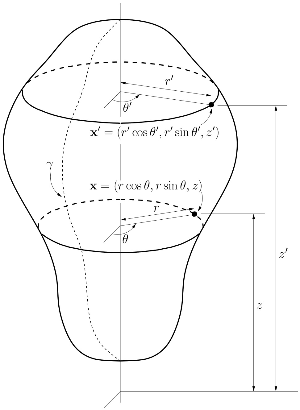
Figure 1.1. The axisymmetric domain $\Gamma$ generated by the curve $\gamma$.

2. Fourier representation of BIE

2.1. Problem formulation

Suppose that $\Gamma$ is a surface in $\mathbb{R}^{3}$ obtained by rotating a smooth contour $\gamma$ about a fixed axis and consider the boundary integral equation

(2.1) $$\sigma({\boldsymbol{x}})+\int_{\Gamma}k(\boldsymbol{x},\boldsymbol{x}^{\prime})\,\sigma(\boldsymbol{x}^{\prime})\,dA(\boldsymbol{x}^{\prime})=f(\boldsymbol{x}),\hskip 10.00002pt\boldsymbol{x}\in\Gamma.$$

In this section, we will demonstrate that if the kernel $k$ is rotationally symmetric in a sense to be made precise, then by taking the Fourier transform in the azimuthal variable, (2.1) can be recast as a sequence of BIEs defined on the curve $\gamma$. To this end, we introduce a Cartesian coordinate system in $\mathbb{R}^{3}$ with the third coordinate axis being the axis of symmetry. Then cylindrical coordinates $(r,z,\theta)$ are defined such that

$$x_{1}= \ r\,\cos\theta,$$

$$x_{2}= \ r\,\sin\theta,$$

$$x_{3}= \ z.$$

Figure 1.1 illustrates the coordinate system.

The kernel $k$ in (2.1) is now rotationally symmetric if for any two points $\boldsymbol{x},\boldsymbol{x}^{\prime}\in\Gamma$,

(2.2) $$k(\boldsymbol{x},\boldsymbol{x}^{\prime})=k(\theta-\theta^{\prime},r,z,r^{\prime},z^{\prime}),$$

where $(\theta^{\prime},r^{\prime},z^{\prime})$ are the cylindrical coordinates of $\boldsymbol{x}^{\prime}$.

2.2. Separation of variables

We define for $n\in\mathbb{Z}$ the functions $f_{n}$, $\sigma_{n}$, and $k_{n}$ via

(2.3) $$f_{n}(r,z) =\int_{\mathbb{T}}\frac{e^{-in\theta}}{\sqrt{2\pi}}\,f(\theta,r,z)\,d\theta,$$

(2.4) $$\sigma_{n}(r,z) =\int_{\mathbb{T}}\frac{e^{-in\theta}}{\sqrt{2\pi}}\,\sigma(\theta,r,z)\,d\theta,$$

(2.5) $$k_{n}(r,z,r^{\prime},z^{\prime}) =\int_{\mathbb{T}}\frac{e^{-in\theta}}{\sqrt{2\pi}}\,k(\theta,r,z,r^{\prime},z^{\prime})\,d\theta.$$

The definitions (2.3), (2.4), and (2.5) define $f_{n}$, $\sigma_{n}$, and $k_{n}$ as the coefficients in the Fourier series of the functions $f$, $\sigma$, and $k$ about the azimuthal variable,

(2.6) $$f(\boldsymbol{x}) =\sum_{n\in\mathbb{Z}}\frac{e^{in\theta}}{\sqrt{2\pi}}\,f_{n}(r,z),$$

(2.7) $$\sigma(\boldsymbol{x}) =\sum_{n\in\mathbb{Z}}\frac{e^{in\theta}}{\sqrt{2\pi}}\,\sigma_{n}(r,z),$$

(2.8) $$k(\boldsymbol{x},\boldsymbol{x}^{\prime})=k(\theta-\theta^{\prime},r,z,r^{\prime},z^{\prime}) =\sum_{n\in\mathbb{Z}}\frac{e^{in(\theta-\theta^{\prime})}}{\sqrt{2\pi}}\,k_{n}(r,z,r^{\prime},z^{\prime}).$$

To determine the Fourier representation of (2.1), we multiply the equation by $e^{-in\theta}/\sqrt{2\pi}$ and integrate $\theta$ over $\mathbb{T}$ (for our purposes, we can think of $\mathbb{T}$ as simply the interval $[-\pi,\,\pi]$). Equation (2.1) can then be said to be equivalent to the sequence of equations

(2.9) $$\sigma_{n}(r,z)+\int_{\gamma\times\mathbb{T}}\left[\int_{\mathbb{T}}\frac{e^{-in\theta}}{\sqrt{2\pi}}\,k(\boldsymbol{x},\boldsymbol{x}^{\prime})\,d\theta\right]\,\sigma(\boldsymbol{x}^{\prime})\,dA(\boldsymbol{x}^{\prime})=f_{n}(r,z),\qquad n\in\mathbb{Z}.$$

Invoking (2.8), we evaluate the bracketed factor in (2.9) as

(2.10) $$\int_{\mathbb{T}}\frac{e^{-in\theta}}{\sqrt{2\pi}}\,k(\boldsymbol{x},\boldsymbol{x}^{\prime})\,d\theta=\int_{\mathbb{T}}\frac{e^{-in\theta}}{\sqrt{2\pi}}\,k(\theta-\theta^{\prime},r,z,r^{\prime},z^{\prime})\,d\theta\\ =e^{-in\theta^{\prime}}\int_{\mathbb{T}}\frac{e^{-in(\theta-\theta^{\prime})}}{\sqrt{2\pi}}\,k(\theta-\theta^{\prime},r,z,r^{\prime},z^{\prime})\,d\theta=e^{-in\theta^{\prime}}\,k_{n}(r,z,r^{\prime},z^{\prime}).$$

Inserting (2.10) into (2.9) and executing the integration of $\theta^{\prime}$ over $\mathbb{T}$, we find that (2.1) is equivalent to the sequence of equations

(2.11) $$\sigma_{n}(r,z)+\sqrt{2\pi}\int_{\gamma}\,k_{n}(r,z,r^{\prime},z^{\prime})\,\sigma_{n}(r^{\prime},z^{\prime})\,r^{\prime}\,dl(r^{\prime},z^{\prime})=f_{n}(r,z),\hskip 10.00002ptn\in\mathbb{Z}.$$

For future reference, we define for $n\in\mathbb{Z}$ the boundary integral operators $\mathcal{K}_{n}$ via

(2.12) $$[\mathcal{K}_{n}\,\sigma_{n}](r,z)=\sqrt{2\pi}\int_{\gamma}k_{n}(r,z,r^{\prime},z^{\prime})\,\sigma_{n}(r^{\prime},z^{\prime})\,r^{\prime}\,dl(r^{\prime},z^{\prime}).$$

Then equation (2.11) can be written

(2.13) $$\bigl{(}I+\mathcal{K}_{n})\,\sigma_{n}=f_{n},\qquad n\in\mathbb{Z}.$$

When each operator $I+\mathcal{K}_{n}$ is continuously invertible, we can write the solution of (2.1) as

(2.14) $$\sigma(r,z,\theta)=\sum_{n\in\mathbb{Z}}\frac{e^{in\theta}}{\sqrt{2\pi}}[(I+\mathcal{K}_{n})^{-1}f_{n}](r,z).$$

2.3. Truncation of the Fourier series

When evaluating the solution operator (2.14) in practice, we will choose a truncation parameter $N_{\rm F}$, and evaluate only the lowest $2N_{\rm F}+1$ Fourier modes. If $N_{\rm F}$ is chosen so that the given function $f$ is well-represented by its lowest $2N_{\rm F}+1$ Fourier modes, then in typical environments the solution obtained by truncating the sum (2.14) will also be accurate. To substantiate this claim, suppose that $\varepsilon$ is a given tolerance, and that $N_{\rm F}$ has been chosen so that

(2.15) $$||f-\sum_{n=-N_{\rm F}}^{N_{\rm F}}\frac{e^{in\theta}}{\sqrt{2\pi}}f_{n}||\leq\varepsilon,$$

We define an approximate solution via

(2.16) $$\sigma_{\textrm{approx}}=\sum_{n=-N_{\rm F}}^{N_{\rm F}}\frac{e^{in\theta}}{\sqrt{2\pi}}(I+\mathcal{K}_{n})^{-1}f_{n}.$$

From Parseval’s identity, we then find that the error in the solution satisfies

$$||\sigma-\sigma_{\textrm{approx}}||^{2}=\sum_{|n|>N_{\rm F}}||(I+\mathcal{K}_{n})^{-1}f_{n}||^{2}\leq\sum_{|n|>N_{\rm F}}||(I+\mathcal{K}_{n})^{-1}||^{2}\,||f_{n}||^{2}$$

$$\leq\left(\max_{|n|>N_{\rm F}}||(I+\mathcal{K}_{n})^{-1}||^{2}\right)\sum_{|n|>N_{\rm F}}||f_{n}||^{2}\leq\left(\max_{|n|>N_{\rm F}}||(I+\mathcal{K}_{n})^{-1}||^{2}\right)\varepsilon^{2}.$$

It is typically the case that the kernel $k(\boldsymbol{x},\boldsymbol{x}^{\prime})$ has sufficient smoothness such that the Fourier modes $k_{n}(r,z,r^{\prime},z^{\prime})$ decay as $n\rightarrow\infty$. Then $||\mathcal{K}_{n}||\rightarrow 0$ as $n\rightarrow\infty$ and $||(I+\mathcal{K}_{n})^{-1}||\rightarrow 1$. Thus, an accurate approximation of $f$ leads to an approximation in $\sigma$ that is of the same order of accuracy. Figure LABEL:fig:cond illustrates that when $k$ is the double layer kernel associated with the Laplace equation, and $\gamma$ is a simple curve, then $||(I+\mathcal{K}_{n})^{-1}||\rightarrow 1$ with rapid convergence.

3. Discretization of BIEs in two dimensions

The technique in Section 2 reduces the BIE (1.1) defined on an axisymmetric surface $\Gamma=\gamma\times\mathbb{T}$ contained in $\mathbb{R}^{3}$, to a sequence of BIEs defined on the curve $\gamma$ contained in $\mathbb{R}^{2}$. These equations take the form

(3.1) $$\sigma(\boldsymbol{x})+\sqrt{2\pi}\int_{\gamma}k_{n}(\boldsymbol{x},\boldsymbol{x}^{\prime})\,\sigma(\boldsymbol{x}^{\prime})\,r^{\prime}\,dl(\boldsymbol{x}^{\prime})=f(\boldsymbol{x}),\qquad\boldsymbol{x}\in\gamma,$$

where the kernel $k_{n}$ is defined as in (2.5). In this section, we describe some standard techniques for discretizing an equation such as (3.1). For simplicity, we limit attention to the case where $\gamma$ is a smooth closed curve, but extensions to non-smooth curves can be handled by slight variations of the techniques described here, [Bremer:a, Bremer:b, Helsing:00a].

3.1. Parameterization of the curve

Let $\gamma$ be parameterized by a vector-valued smooth function $\boldsymbol{\tau}:[0,T]\rightarrow\mathbb{R}^{2}$. The parameterization converts (3.1) to an integral equation defined on the interval $[0,T]$:

(3.2) $$\sigma(\boldsymbol{\tau}(t))+\sqrt{2\pi}\int_{0}^{T}k_{n}(\boldsymbol{\tau}(t),\boldsymbol{\tau}(s))\,\sigma(\boldsymbol{\tau}(s))\,r^{\prime}(\boldsymbol{\tau}(s))\,|d\boldsymbol{\tau}/ds|\,ds=f(\boldsymbol{\tau}(t)),\qquad t\in[0,T].$$

To keep our formulas uncluttered, we suppress the parameterization of the curve and the dependence on $n$ and introduce a new kernel

(3.3) $$K(t,s)=\sqrt{2\pi}\,k_{n}(\boldsymbol{\tau}(t),\boldsymbol{\tau}(s))\,r^{\prime}(\boldsymbol{\tau}(s))\,|d\boldsymbol{\tau}/ds|,$$

as well as the functions

$$\varphi(t)=\sigma(\boldsymbol{\tau}(t))\hskip 10.00002pt\textrm{and}\hskip 10.00002pt\psi(t)=f(\boldsymbol{\tau}(t)).$$

Then techniques for solving

(3.4) $$\varphi(t)+\int_{0}^{T}K(t,s)\,\varphi(s)\,ds=\psi(t),\qquad t\in[0,T],$$

where $\psi$ is given and $\varphi$ is to be determined, will be equally applicable to (3.2).

3.2. Nyström method

We will discretize (3.4) via Nyström discretization on standard Gaussian quadrature nodes, see [Atkinson:97a]. To this end, we divide the interval $\Omega=[0,T]$ into a disjoint partition of $N_{\rm P}$ intervals,

$$\Omega=\bigcup_{p=1}^{N_{\rm P}}\Omega_{p},$$

where each $\Omega_{p}$ is a subinterval called a panel. On each panel $\Omega_{p}$, we place the nodes of a standard $N_{\rm G}$-point Gaussian quadrature rule $\{t_{i}^{(p)}\}_{i=1}^{N_{\rm G}}$. The idea is now to enforce (3.4) at each of the $N_{\rm P}N_{\rm G}$ nodes:

$$\sigma(t_{i}^{(p)})+\int_{0}^{T}K(t_{i}^{(p)},s)\,\varphi(s)\,ds=\psi(t_{i}^{(p)}),\qquad(i,p)\in\{1,2,\ldots,N_{\rm G}\}\times\{1,2,\ldots,N_{\rm P}\}.$$

To obtain a numerical method, suppose that we can construct for $p,q\in\{1,\,2,\,\dots,\,N_{\rm P}\}$ and $i,j\in\{1,\,2,\,\dots,\,N_{\rm G}\}$ numbers $A_{i,j}^{(p,q)}$ such that

(3.5) $$\int_{0}^{T}K(t_{i}^{(p)},s)\,\varphi(s)\,ds\approx\sum_{q=1}^{N_{\rm P}}\sum_{j=1}^{N_{\rm G}}A_{i,j}^{(p,q)}\,\varphi(t_{j}^{(q)}).$$

Then the Nyström method is given by solving the linear system

(3.6) $$\varphi_{i}^{(p)}+\sum_{q=1}^{N_{\rm P}}\sum_{j=1}^{N_{\rm G}}A_{i,j}^{(p,q)}\,\varphi_{j}^{(q)}=\psi_{i}^{(p)},\qquad(i,p)\in\{1,2,\ldots,N_{\rm G}\}\times\{1,2,\ldots,N_{\rm P}\},$$

where $\psi_{i}^{(p)}=\psi(t_{i}^{(p)})$ and $\varphi_{i}^{(p)}$ approximates $\varphi(t_{i}^{(p)})$. We write (3.6) compactly as

$$(I+A)\,\varphi=\psi$$

where $A$ is a matrix formed by $N_{\rm P}\times N_{\rm P}$ blocks, each of size $N_{\rm G}\times N_{\rm G}$. We let $A^{(p,q)}$ denote the block of $A$ representing the interactions between the panels $\Omega_{p}$ and $\Omega_{q}$.

3.3. Quadrature and interpolation

We need to determine the numbers $A_{i,j}^{(p,q)}$ such that (3.5) holds. The detailed construction is given in Section 3.4, and utilizes some well-known techniques of quadrature and interpolation, which we review in this section.

3.3.1. Standard Gaussian quadratures

Given an interval $[0,\,h]$ and a positive integer $N_{\rm G}$, the $N_{\rm G}$-point standard Gaussian quadrature rule consists of a set of $N_{\rm G}$ nodes $\{t_{j}\}_{j=1}^{N_{\rm G}}\subset[0,\,h]$, and $N_{\rm G}$ weights $\{w_{j}\}_{j=1}^{N_{\rm G}}$ such that

$$\int_{0}^{h}g(s)\,ds=\sum_{j=1}^{N_{\rm G}}w_{j}\,g(t_{j}),$$

whenever $g$ is a polynomial of degree at most $2N_{\rm G}-1$, and such that

$$\int_{0}^{h}g(s)\,ds=\sum_{j=1}^{N_{\rm G}}w_{j}\,g(t_{j})+O(h^{2N_{\rm G}}),$$

whenever $g$ is a function with $2N_{\rm G}$ continuous derivatives, see [Abramowitz:65a].

3.3.2. Quadrature rules for singular functions

Now suppose that given an interval $[0,\,h]$ and a point $t\in[-h,\,2h]$, we seek to integrate over $[0,\,h]$ functions $g$ that take the form

(3.7) $$g(s)=\phi_{1}(s)\log|s-t|+\phi_{2}(s),$$

where $\phi_{1}$ and $\phi_{2}$ are polynomials of degree at most $2N_{\rm G}-1$. Standard Gaussian quadrature would be highly inaccurate if applied to integrate (3.7). Rather, seek a $N_{\rm{G}}^{\prime}$-node quadrature that will evaluate

(3.8) $$\int_{0}^{h}g(s)\,ds$$

exactly. Techniques for constructing such generalized quadratures are readily available in the literature, see for example [Kolm:01a]. These quadratures will be of degree $2N_{\rm G}-1$, just as with standard Gaussian quadratures and exhibit comparable accuracy, although in general $N_{\rm{G}}^{\prime}>N_{\rm G}$. The generalized quadratures used in this paper were determined using the techniques of [Kolm:01a], and can be found in the appendix.

We observe that the quadrature nodes constructed by such methods are typically different from the nodes of the standard Gaussian quadrature. This complicates the the construction of the matrix $A$, as described in Section 3.4.

3.3.3. Lagrange interpolation

Let $\{t_{j}\}_{j=1}^{N_{\rm G}}$ denote the nodes of a $N_{\rm G}$-point Gaussian quadrature rule on the interval $[0,h]$. If the values of a polynomial $g$ of degree at most $N_{\rm G}-1$ are specified at these nodes, the entire polynomial $g$ can be recovered via the formula

$$g(s)=\sum_{j=1}^{N_{\rm G}}L_{j}(s)\,g(t_{j}),$$

where the functions $L_{j}$ are the Lagrange interpolating polynomials

$$L_{j}(s)=\prod_{i\neq j}\left(\frac{s-t_{i}}{t_{j}-t_{i}}\right).$$

If $g$ is a smooth function with $N_{\rm G}$ continuous derivatives that is not a polynomial, then the Lagrange interpolant provides an approximation to $g$ satisfying

$$\left|g(s)-\sum_{j=1}^{N_{\rm G}}L_{j}(s)\,g(t_{j})\right|\leq C\,h^{N_{\rm G}},$$

where

$$C=\left({\displaystyle\sup_{s\in[0,h]}}|g^{(N_{\rm G})}(s)|\right)/N_{\rm G}!.$$

3.4. Constructing the matrix $A$

Using the tools reviewed in Section 3.3, we are now in position to construct numbers $A_{i,j}^{(p,q)}$ such that (3.5) holds. We first note that in forming block $A^{(p,q)}$ of $A$, we need to find numbers $A_{i,j}^{(p,q)}$ such that

(3.9) $$\int_{\Omega_{q}}K(t_{i}^{(p)},s)\,\varphi(s)\,ds\approx\sum_{j=1}^{N_{\rm G}}A_{i,j}^{(p,q)}\,\varphi(t_{j}^{(q)}),\qquad i=1,\,2,\,\dots,\,N_{\rm G}.$$

When $\Omega_{p}$ and $\Omega_{q}$ are well separated, the integrand in (3.9) is smooth, and our task is easily solved using standard Gaussian quadrature (as described in Section 3.3.1):

$$\int_{\Omega_{q}}K(t_{i}^{(p)},s)\,\varphi(s)\,ds\approx\sum_{j=1}^{N_{\rm G}}w_{j}\,K(t_{i}^{(p)},t_{j}^{(q)})\,\varphi(t_{j}^{(q)}).$$

It directly follows that the $ij$ entry of the block $A^{(p,q)}$ takes the form

(3.10) $$A^{(p,q)}_{i,j}=w_{j}\,K(t_{i}^{(p)},\,t_{j}^{(q)}).$$

Complications arise when we seek to form a diagonal block $A^{(p,p)}$, or even a block that is adjacent to a diagonal block. The difficulty is that the kernel $K(t,s)$ has a singularity as $s\rightarrow t$. To be precise, for any fixed $t$, there exist smooth functions $u_{t}$ and $v_{t}$ such that

$$K(t,s)=\log|t-s|\,u_{t}(s)+v_{t}(s).$$

We see that when $t_{i}^{(p)}$ is a point in $\Omega_{q}$ the integrand in (3.9) becomes singular. When $t_{i}^{(p)}$ is a point in a panel neighboring $\Omega_{q}$, the problem is less severe, but Gaussian quadrature would still be inaccurate. To maintain full accuracy, we use the modified quadrature rules described in Section 3.3.2. For every node $t_{i}^{(p)}\in\Omega_{p}$, we construct a quadrature $\{\hat{w}_{i,\ell}^{(p,q)},\hat{t}^{(p,q)}_{i,\ell}\}_{\ell=1}^{N_{\rm{G}}^{\prime}}$ such that

(3.11) $$\int_{\Omega_{q}}K(t_{i}^{(p)},s)\,\varphi(s)\,ds\approx\sum_{\ell=1}^{N_{\rm{G}}^{\prime}}\hat{w}_{i,\ell}^{(p,q)}\,K(t_{i}^{(p)},\hat{t}_{i,\ell}^{(p,q)})\,\varphi(\hat{t}_{i,\ell}^{(p,q)}).$$

In order to have a quadrature evaluated at the Gaussian nodes $t_{j}^{(q)}\in\Omega_{q}$, we next use Lagrange interpolation as described in Section 3.3.3. With $\{L_{j}^{(q)}\}_{j=1}^{N_{\rm G}}$ denoting the Lagrange interpolants of order $N_{\rm G}-1$ defined on $\Omega_{q}$, we have

(3.12) $$\varphi(t)\approx\sum_{j=1}^{N_{\rm G}}L_{j}^{(q)}(t)\,\varphi(t_{j}^{(q)}),\qquad t\in\Omega_{q}.$$

Inserting (3.12) into (3.11), we find that

$$\int_{\Omega_{q}}K(t_{i}^{(p)},s)\,\varphi(s)\,ds\approx\sum_{\ell=1}^{N_{\rm{G}}^{\prime}}\hat{w}_{i,\ell}^{(p,q)}\,K(t_{i}^{(p)},\hat{t}_{i,\ell}^{(p,q)})\,\sum_{j=1}^{N_{\rm G}}L_{j}^{(q)}(\hat{t}_{i,\ell}^{(p,q)})\,\varphi(t_{j}^{(q)}).$$

We now find that the block $A^{(p,q)}$ of $A$ has entries

(3.13) $$A^{(p,q)}_{i,j}=\sum_{\ell=1}^{N_{\rm{G}}^{\prime}}\hat{w}_{i,\ell}^{(p,q)}\,K(t_{i}^{(p)},\hat{t}_{i,\ell}^{(p,q)})\,L_{j}^{(q)}(\hat{t}_{i,\ell}^{(p,q)}),\qquad i,j\in\{1,2,\ldots,N_{G}\}.$$

We observe that the formula (3.13) is quite expensive to evaluate; in addition to the summation, it requires the construction of a quadrature rule for each point $t_{i}^{(p)}$ and evaluation of Lagrange interpolants. Fortunately, this process must be executed for at most three blocks in each row of blocks of $A$.

4. A general algorithm

4.1. Summary

At this point, we have shown how to convert a BIE defined on an axisymmetric surface in $\mathbb{R}^{3}$ to a sequence of equations defined on a curve in $\mathbb{R}^{2}$ (Section 2), and then how to discretize each of these reduced equations (Section 3). Putting everything together, we obtain the following algorithm for solving (1.1):

1. Given the right hand side $f$, and a computational tolerance $\varepsilon$, determine a truncation parameter $N_{\rm F}$ such that (2.15) holds.

2. Form for $n=-N_{\rm F},\,-N_{\rm F}\,+1,\,-N_{\rm F}+2,\,\dots,\,N_{\rm F}$ the matrix $A_{n}$ discretizing the equation (2.13) encapsulating the $n$’th Fourier mode. The matrix is formed via Nyström discretization as described in Section 3 with the discretization parameters $N_{\rm P}$ and $N_{\rm G}$ chosen to meet the computational tolerance $\varepsilon$.

3. Evaluate via the FFT the terms $\{f_{n}\}_{n=-N_{\rm F}}^{N_{\rm F}}$ in the Fourier representation of $f$ (as defined by (2.3)), and solve for $n=-N_{\rm F},\,-N_{\rm F}+1,\,-N_{\rm F}+2,\,\dots,\,N_{\rm F}$ the equation $(I+A_{n})\,\sigma_{n}=f_{n}$ for $\sigma_{n}$. Construct $\sigma_{\rm approx}$ using formula (2.16) evaluated via the FFT.

The construction of the matrices $A_{n}$ in Step 2 can be accelerated using the FFT (as described in Section 4.2), but even with such acceleration, it is typically by a wide margin the most expensive part of the algorithm. However, this step needs to be performed only once for any given geometry, and given discretization parameters $N_{\rm F}$, $N_{\rm P}$, and $N_{\rm G}$. The method therefore becomes particularly efficient when (1.1) needs to be solved for a sequence of right-hand sides. In this case, it may be worth the cost to pre-compute the inverse of each matrix $I+A_{n}$.

4.2. Techniques for forming the matrices

We need to construct for each Fourier mode $n$, a matrix $A_{n}$ consisting of $N_{\rm P}\times N_{\rm P}$ blocks $A_{n}^{(p,q)}$, each of size $N_{\rm G}\times N_{\rm G}$. Constructing an off-diagonal block $A_{n}^{(p,q)}$ when $\Omega_{p}$ and $\Omega_{q}$ are not directly adjacent is relatively straightforward. For any pair of nodes $t_{i}^{(p)}\in\Omega_{p}$ and $t_{j}^{(q)}\in\Omega_{q}$, we need to construct the numbers, cf. (3.3) and (3.10),

(4.1) $$A^{(p,q)}_{n;i,j}=\sqrt{2\pi}\,w_{j}\,k_{n}(\boldsymbol{\tau}(t_{i}^{(p)}),\,\boldsymbol{\tau}(t_{j}^{(q)}))\,r^{\prime}(\boldsymbol{\tau}(t_{j}^{(q)}))\,|d\boldsymbol{\tau}(t_{j}^{(q)})/ds|,$$

for $n=-N_{\rm F},\,-N_{\rm F}+1,\,\dots,\,N_{\rm F}$, where $\boldsymbol{\tau}$ is a parameterization of $\gamma$ (see Section 3.1) and the kernel $k_{n}$ is defined by (2.5). Fortunately, we do not need to explicitly evaluate the integrals in (2.5) since all the $2N_{\rm F}+1$ numbers can be evaluated by a single application of the FFT to the function

(4.2) $$\theta\mapsto k(\theta,\,\boldsymbol{\tau}(t_{i}^{(p)}),\,\boldsymbol{\tau}(t_{j}^{(q)})).$$

When $\boldsymbol{\tau}(t_{i}^{(p)})$ is not close to $\boldsymbol{\tau}(t_{j}^{(q)})$, the function in (4.2) is smooth, and the trapezoidal rule implicit in applying the FFT is highly accurate.

Evaluating the blocks on the diagonal, or directly adjacent to the diagonal is somewhat more involved. The matrix entries are now given by the formula, cf. (3.3) and (3.13),

(4.3) $$A^{(p,q)}_{k;i,j}=\sum_{\ell=1}^{N_{\rm{G}}^{\prime}}\hat{w}_{i,\ell}^{(p,q)}\,k_{n}(\boldsymbol{\tau}(t_{i}^{(p)}),\boldsymbol{\tau}(\hat{t}_{i,\ell}^{(p,q)}))\,r^{\prime}(\hat{t}_{i,\ell}^{(p,q)})\,|d\boldsymbol{\tau}(\hat{t}_{i,\ell}^{(p,q)})/ds|\,L_{j}^{(q)}(\hat{t}_{i,\ell}^{(p,q)}),$$

where $\boldsymbol{\tau}$ and $k_{n}$ are as in (4.1). To further complicate things, the points $\boldsymbol{\tau}(t_{i}^{(p)})$ and $\boldsymbol{\tau}(\hat{t}_{i,\ell}^{(p,q)})$ are now in close proximity to each other, and so the functions

(4.4) $$\theta\mapsto k(\theta,\,\boldsymbol{\tau}(t_{i}^{(p)}),\,\boldsymbol{\tau}(\hat{t}_{i,\ell}^{(p,q)}))$$

have a sharp peak around the point $\theta=0$. They are typically still easy to integrate away from the origin, so the integrals in (2.5) can for a general kernel be evaluated relatively efficiently using quadratures that are adaptively refined near the origin.

Even with the accelerations described in this section, the cost of forming the matrices $A_{n}$ tends to dominate the computation whenever the kernels $k_{n}$ must be evaluated via formula (2.5). In particular environments, it is possible to side-step this problem by evaluating the integral in (2.5) analytically. That this can be done for the single and double layer kernels associated with Laplace’s equation is demonstrated in Section 5.

4.3. Computational costs

The asymptotic cost of the algorithm described in Section 4.1 has three components: (a) the cost of forming the matrices $\{A_{n}\}_{n=-N_{\rm F}}^{N_{\rm F}}$, (b) the cost of transforming functions from physical space to Fourier space and back, and (c) the cost of solving the linear systems $(I+A_{n})\,\sigma_{n}=f_{n}$. In this section, we investigate the asymptotic cost of these steps. We consider a situation where $N_{\rm F}$ Fourier modes need to be resolved, and where $N_{\rm P}\times N_{\rm G}$ nodes are used to discretize the curve $\gamma$.

(a) Cost of forming the linear systems: Suppose first that we have an analytic formula for each kernel $k_{n}$. (As we do, e.g., when the original BIE (1.1) involves either the single or the double layer kernel associated with Laplace’s equation, see Section 5.) Then the cost $T_{\rm mat}$ of forming the matrices satisfies

$$T_{\rm mat}\hskip 20.00003pt\sim\underbrace{N_{\rm P}^{2}\,N_{\rm G}^{2}\,N_{\rm F}}_{\textrm{cost from kernel evaluations}}\hskip 5.0pt+\underbrace{N_{\rm P}\,N_{\rm G}^{3}\,N_{\rm F}}_{\textrm{cost from composite quadrature}}.$$

When the kernels have to be evaluated numerically via formula (2.5), the cost of forming the matrices is still moderate. In the rare situations where the kernel is smooth, standard Gaussian quadrature can be used everywhere and the FFT acceleration described in Section 4.2 can be used for all entries. In this situation,

$$T_{\rm mat}\sim N_{\rm P}^{2}\,N_{\rm G}^{2}\,N_{\rm F}\,\log(N_{\rm F}).$$

In the more typical situation where each kernel $k_{n}$ involves an integrable singularity at the diagonal, the FFT acceleration can still be used to rapidly evaluate all entries well-removed from the diagonal. However, entries close to the diagonal must be formed via the composite quadrature rule combined with numerical evaluation of $k_{n}$ via an adaptive quadrature. In this situation,

$$T_{\rm mat}\sim N_{\rm P}^{2}\,N_{\rm G}^{2}\,N_{\rm F}\,\log(N_{\rm F})+N_{\rm P}\,N_{\rm G}^{3}\,N_{\rm F}^{2}.$$

(b) Cost of Fourier transforms: The boundary data defined on the surface must be converted into the Fourier domain. This is executed via the FFT at a cost $T_{\rm fft}$ satisfying

(4.5) $$T_{\rm fft}\sim N_{\rm P}\,N_{\rm G}\,N_{\rm F}\,\log(N_{\rm F}).$$

We observe that the constant of proportionality in (4.5) is very small, and the cost of this step is typically negligible compared to the costs of the other steps.

(c) Cost of linear solves: Using standard Gaussian elimination, the cost $T_{\rm solve}$ of solving $N_{\rm F}$ linear systems $(I+A_{n})\,\sigma_{n}=f_{n}$, each of size $N_{\rm P}\,N_{\rm G}\times N_{\rm P}\,N_{\rm G}$, satisfies

$$T_{\rm solve}\sim N_{\rm P}^{3}\,N_{\rm G}^{3}\,N_{\rm F}.$$

In situations where the equations need to be solved for multiple right hand sides, it pays off to first compute the inverses $(I+A_{n})^{-1}$, and then simply apply these to each right hand side (or, alternatively, to form the LU factorizations, and then perform triangular solves). The cost $T_{\rm inv}$ of computing the inverses, and the cost $T_{\rm apply}$ of applying them then satisfy

$$T_{\rm inv} \sim N_{\rm P}^{3}\,N_{\rm G}^{3}\,N_{\rm F},$$

$$T_{\rm apply} \sim N_{\rm P}^{2}\,N_{\rm G}^{2}\,N_{\rm F}.$$

We make some practical observations:

• The cost of forming the matrices by far dominates the other costs unless the kernel is either smooth, or analytic formulas for $k_{n}$ are available.

• The scheme is highly efficient in situations where the same equation needs to be solved for a sequence of different right hand sides. Given an additional right hand side, the added cost $T_{\rm solve}$ is given by

  $$T_{\rm solve}\sim N_{\rm P}\,N_{\rm G}\,N_{\rm F}\,\log(N_{\rm F})+N_{\rm P}^{2}\,N_{\rm G}^{2}\,N_{\rm F},$$

  with a very small constant of proportionality. We note that this cost remains small even if an analytic formula for $k_{n}$ is not available.

• The system matrices $I+A_{n}$ often have internal structure that allow them to be inverted using “fast methods” such as, e.g., those in [Martinsson:04a]. The cost of inversion and application can then be accelerated to near optimal complexity.

5. Simplifications for the double layer kernels associated with Laplace’s equation

5.1. The double layer kernels of Laplace’s equation

Let $D\subseteq\mathbb{R}^{3}$ be a bounded domain whose boundary is given by a smooth surface $\Gamma$, let $E=\bar{D}^{\rm c}$ denote the domain exterior to $D$, and let $\boldsymbol{n}$ and be the outward unit normal to $D$. Consider the interior and exterior Dirichlet problems of potential theory [Guenther:88a],

(5.1) $$\Delta u=0\hskip 5.0pt\textrm{in}\hskip 5.0ptD,\hskip 10.00002ptu=f\hskip 5.0pt\textrm{on}\hskip 5.0pt\Gamma,\hskip 20.00003pt\textrm{(interior Dirichlet problem)}$$

(5.2) $$\Delta u=0\hskip 5.0pt\textrm{in}\hskip 5.0ptE,\hskip 10.00002ptu=f\hskip 5.0pt\textrm{on}\hskip 5.0pt\Gamma.\hskip 20.00003pt\textrm{(exterior Dirichlet problem)}$$

The solutions to (5.1) and (5.2) can be written in the respective forms

$$u(\boldsymbol{x})=\int_{\Gamma}\frac{\boldsymbol{n}(\boldsymbol{x}^{\prime})\cdot(\boldsymbol{x}-\boldsymbol{x}^{\prime})}{4\pi|\boldsymbol{x}-\boldsymbol{x}^{\prime}|^{3}}\sigma(\boldsymbol{x}^{\prime})\,dA(\boldsymbol{x}^{\prime}),\hskip 10.00002pt\boldsymbol{x}\in D,$$

$$u(\boldsymbol{x})=\int_{\Gamma}\left(-\frac{\boldsymbol{n}(\boldsymbol{x}^{\prime})\cdot(\boldsymbol{x}-\boldsymbol{x}^{\prime})}{4\pi|\boldsymbol{x}-\boldsymbol{x}^{\prime}|^{3}}+\frac{1}{4\pi|\boldsymbol{x}-\boldsymbol{x}_{0}|}\right)\sigma(\boldsymbol{x}^{\prime})\,dA(\boldsymbol{x}^{\prime}),\hskip 10.00002pt\boldsymbol{x}\in E,\hskip 5.0pt\boldsymbol{x}_{0}\in D,$$

where $\sigma$ is a boundary charge distribution that can be determined using the boundary conditions. The resulting equations are

(5.3) $$-\frac{1}{2}\sigma(\boldsymbol{x}) +\int_{\Gamma}\frac{\boldsymbol{n}(\boldsymbol{x}^{\prime})\cdot(\boldsymbol{x}-\boldsymbol{x}^{\prime})}{4\pi|\boldsymbol{x}-\boldsymbol{x}^{\prime}|^{3}}\sigma(\boldsymbol{x}^{\prime})\,dA(\boldsymbol{x}^{\prime})=f(\boldsymbol{x}),\hskip 10.00002pt\boldsymbol{x}\in\Gamma,$$

(5.4) $$-\frac{1}{2}\sigma(\boldsymbol{x}) +\int_{\Gamma}\left(-\frac{\boldsymbol{n}(\boldsymbol{x}^{\prime})\cdot(\boldsymbol{x}-\boldsymbol{x}^{\prime})}{4\pi|\boldsymbol{x}-\boldsymbol{x}^{\prime}|^{3}}+\frac{1}{4\pi|\boldsymbol{x}-\boldsymbol{x}_{0}|}\right)\sigma(\boldsymbol{x}^{\prime})\,dA(\boldsymbol{x}^{\prime})=f(\boldsymbol{x}),\hskip 10.00002pt\boldsymbol{x}\in\Gamma.$$

Remark 5.1.

There are other integral formulations for the solution to Laplace’s equation. The double layer formulation presented here is a good choice in that it provides an integral operator that leads to well conditioned linear systems. However, the methodology of this paper is equally applicable to single-layer formulations that lead to first kind Fredholm BIEs.

5.2. Separation of variables

Using the procedure given in Section 2, if $\Gamma=\gamma\times\mathbb{T}$, then (5.1) and (5.2) can be recast as a series of BIEs defined along $\gamma$. We express $\boldsymbol{n}$ in cylindrical coordinates as

$$\boldsymbol{n}(\boldsymbol{x}^{\prime})=(n_{r^{\prime}}\cos\theta^{\prime},n_{r^{\prime}}\sin\theta^{\prime},n_{z^{\prime}}).$$

Further,

$$|\boldsymbol{x}-\boldsymbol{x}^{\prime}|^{2} =(r\cos\theta-r^{\prime}\cos\theta^{\prime})^{2}+(r\sin\theta-r^{\prime}\sin\theta^{\prime})^{2}+(z-z^{\prime})^{2}$$

$$=r^{2}+(r^{\prime})^{2}-2rr^{\prime}(\sin\theta\sin\theta^{\prime}+\cos\theta\cos\theta^{\prime})+(z-z^{\prime})^{2}$$

$$=r^{2}+(r^{\prime})^{2}-2rr^{\prime}\cos(\theta-\theta^{\prime})+(z-z^{\prime})^{2}$$

and

$$\boldsymbol{n}(\boldsymbol{x}^{\prime})\cdot(\boldsymbol{x}-\boldsymbol{x}^{\prime}) =(n_{r^{\prime}}\cos\theta^{\prime},n_{r^{\prime}}\sin\theta^{\prime},n_{z^{\prime}})\cdot(r\cos\theta-r^{\prime}\cos\theta^{\prime},r\sin\theta-r^{\prime}\sin\theta^{\prime},z-z^{\prime})$$

$$=n_{r^{\prime}}r(\sin\theta\sin\theta^{\prime}+\cos\theta\cos\theta^{\prime})-n_{r^{\prime}}r^{\prime}+n_{z^{\prime}}(z-z^{\prime})$$

$$=n_{r^{\prime}}(r\cos(\theta-\theta^{\prime})-r^{\prime})+n_{z^{\prime}}(z-z^{\prime}).$$

Then for a point $\boldsymbol{x}^{\prime}\in\Gamma$, the kernel of the internal Dirichlet problem can be expanded as

$$\frac{\boldsymbol{n}(\boldsymbol{x}^{\prime})\cdot(\boldsymbol{x}-\boldsymbol{x}^{\prime})}{4\pi|\boldsymbol{x}-\boldsymbol{x}^{\prime}|^{3}}=\frac{1}{\sqrt{2\pi}}\sum_{n\in\mathbb{Z}}e^{in(\theta-\theta^{\prime})}d^{(i)}_{n}(r,z,r^{\prime},z^{\prime}),$$

where

$$d^{(i)}_{n}(r,z,r^{\prime},z^{\prime})=\frac{1}{\sqrt{32\pi^{3}}}\int_{\mathbb{T}}e^{-in\theta}\left[\frac{n_{r^{\prime}}(r\cos\theta-r^{\prime})+n_{z^{\prime}}(z-z^{\prime})}{(r^{2}+(r^{\prime})^{2}-2rr^{\prime}\cos\theta+(z-z^{\prime})^{2})^{3/2}}\right]\,d\theta.$$

Similarly, the kernel of the external Dirichlet problem can be written as

$$-\frac{\boldsymbol{n}(\boldsymbol{x}^{\prime})\cdot(\boldsymbol{x}-\boldsymbol{x}^{\prime})}{4\pi|\boldsymbol{x}-\boldsymbol{x}^{\prime}|^{3}}+\frac{1}{4\pi|\boldsymbol{x}-\boldsymbol{x}_{0}|}=\frac{1}{\sqrt{2\pi}}\sum_{n\in\mathbb{Z}}e^{in(\theta-\theta^{\prime})}d^{(e)}_{n}(r,z,r^{\prime},z^{\prime}),$$

with

$$d^{(e)}_{n}(r,z,r^{\prime},z^{\prime})=\frac{1}{\sqrt{32\pi^{3}}} \int_{\mathbb{T}}e^{-in\theta}\biggl{(}-\frac{n_{r^{\prime}}(r\cos\theta-r^{\prime})+n_{z^{\prime}}(z-z^{\prime})}{(r^{2}+(r^{\prime})^{2}-2rr^{\prime}\cos\theta+(z-z^{\prime})^{2})^{3/2}}+$$

$$+\frac{1}{(r^{2}+r_{0}^{2}-2rr_{0}\cos\theta+(z-z_{0})^{2})^{1/2}}\biggr{)}\,d\theta,$$

where $\boldsymbol{x}_{0}$ has been written in cylindrical coordinates as $(r_{0}\cos(\theta_{0}),r_{0}\sin(\theta_{0}),z_{0})$. With the expansions of the kernels available, the procedure described in Section 4 can be used to solve (5.3) and (5.4) by solving

(5.5) $$\sigma_{n}(r,z)+\sqrt{2\pi}\int_{\gamma}d^{(i)}_{n}(r,r^{\prime},z,z^{\prime})\sigma_{n}(r^{\prime},z^{\prime})\,r^{\prime}\,dl(r^{\prime},z^{\prime})=f_{n}(r,z)$$

and

(5.6) $$\sigma_{n}(r,z)+\sqrt{2\pi}\int_{\gamma}d^{(e)}_{n}(r,r^{\prime},z,z^{\prime})\sigma_{n}(r^{\prime},z^{\prime})\,r^{\prime}\,dl(r^{\prime},z^{\prime})=f_{n}(r,z),$$

respectively for $n=-N_{\rm{F}},-N_{\rm{F}}+1,\ldots,N_{\rm{F}}$. Note that the kernels $d^{(i)}_{n}$ and $d^{(e)}_{n}$ contain a log-singularity when both $r^{\prime}=r$ and $z^{\prime}=z$.

Equivalently, (5.5) and (5.6) can be arrived at by considering Laplace’s equation written in cylindrical coordinates,

$$\frac{\partial^{2}u}{\partial^{2}r}+\frac{1}{r}\frac{\partial u}{\partial r}+\frac{1}{r^{2}}\frac{\partial^{2}u}{\partial^{2}\theta}+\frac{\partial^{2}u}{\partial^{2}z}=0,$$

Taking the Fourier transform of $u$ with respect to theta $\theta$ gives

$$\frac{\partial^{2}u_{n}}{\partial^{2}r}+\frac{1}{r}\frac{\partial u_{n}}{\partial r}-\frac{n^{2}}{r^{2}}\frac{\partial^{2}u_{n}}{\partial^{2}\theta}+\frac{\partial^{2}u_{n}}{\partial^{2}z}=0,\hskip 10.00002ptn\in\mathbb{Z},$$

where $e_{n}=e_{n}(\theta)=e^{in\theta}/\sqrt{2\pi}$ and $u=\displaystyle\sum_{n\in\mathbb{Z}}e_{n}u_{n}$. Then (5.5) and (5.6) are now associated with this sequence of PDEs.

5.3. Evaluation of kernels

The values of $d^{(i)}_{n}$ and $d^{(e)}_{n}$ for $n=-N_{\rm{F}},-N_{\rm{F}}+1,\ldots,N_{\rm{F}}$ need to be computed efficiently and with high accuracy to construct the Nyström discretization of (5.5) and (5.6). Note that the integrands of $d^{(i)}_{n}$ and $d^{(e)}_{n}$ are real valued and even functions on the interval $[-\pi,\pi]$. Therefore, $d^{(i)}_{n}$ can be written as

(5.7) $$d_{n}^{(i)}(r,z,r^{\prime},z^{\prime})=\frac{1}{\sqrt{32\pi^{3}}}\int_{\mathbb{T}}\left[\frac{n_{r^{\prime}}(r\cos t-r^{\prime})+n_{z^{\prime}}(z-z^{\prime})}{(r^{2}+(r^{\prime})^{2}-2rr^{\prime}\cos t+(z-z^{\prime})^{2})^{3/2}}\right]\cos(nt)\,dt.$$

Note that $d^{(e)}_{n}$ can be written in a similar form.

This integrand is oscillatory and increasingly peaked at the origin as both $r^{\prime}\rightarrow r$ and $z^{\prime}\rightarrow z$. As long as $r^{\prime}$ and $r$ as well as $z^{\prime}$ and $z$ are well separated, the integrand does not experience peaks near the origin, and as mentioned before, the FFT provides a fast and accurate way for calculating $d^{(i)}_{n}$ and $d^{(e)}_{n}$.

In regimes where the integrand is peaked, the FFT no longer provides a means of evaluating $d^{(i)}_{n}$ and $d^{(e)}_{n}$ with the desired accuracy. One possible solution to this issue is applying adaptive quadrature to fully resolve the peak. However, this must be done for each value of $n$ required and becomes prohibitively expensive if $N_{\rm{F}}$ is large.

Fortunately, an analytical solution to (5.7) exists. As noted in [Cohl:99a], the single-layer kernel can be expanded with respect to the azimuthal variable as

$$s(\boldsymbol{x},\boldsymbol{x}^{\prime})=\frac{1}{4\pi|\boldsymbol{x}-\boldsymbol{x}^{\prime}|}=\frac{1}{4\pi^{2}\sqrt{rr^{\prime}}}\sum_{n\in\mathbb{Z}}e^{in(\theta-\theta^{\prime})}\mathcal{Q}_{n-1/2}(\chi),$$

where $\mathcal{Q}_{n-1/2}$ is the half-integer degree Legendre function of the second kind and

$$\chi=\frac{r^{2}+(r^{\prime})^{2}+(z-z^{\prime})^{2}}{2rr^{\prime}}.$$

In light of this expansion, single-layer kernel can similarly be written as

$$s(\boldsymbol{x},\boldsymbol{x}^{\prime}) =\frac{1}{4\pi(r^{2}+(r^{\prime})^{2}-2rr^{\prime}\cos(\theta-\theta^{\prime})+(z-z^{\prime})^{2})^{1/2}}$$

$$=\frac{1}{\sqrt{2\pi}}\sum_{n\in\mathbb{Z}}e^{in(\theta-\theta^{\prime})}s_{n}(r,z,r^{\prime},z^{\prime})$$

where

$$s_{n}(r,z,r^{\prime},z^{\prime}) =\frac{1}{\sqrt{32\pi^{3}}}\int_{\mathbb{T}}\frac{\cos(nt)}{(r^{2}+(r^{\prime})^{2}-2rr^{\prime}\cos(t)+(z-z^{\prime})^{2})^{1/2}}\,dt$$

$$=\frac{1}{\sqrt{8\pi^{3}rr^{\prime}}}\int_{\mathbb{T}}\frac{\cos(nt)}{\sqrt{8(\chi-\cos(t))}}\,dt$$

$$=\frac{1}{\sqrt{8\pi^{3}rr^{\prime}}}\mathcal{Q}_{n-1/2}(\chi).$$

To find an analytical form for (5.7), first note that in cylindrical coordinates the double-layer kernel can be written in terms of the single-layer kernel,

$$\frac{\boldsymbol{n}(\boldsymbol{x}^{\prime})\cdot(\boldsymbol{x}-\boldsymbol{x}^{\prime})}{4\pi|\boldsymbol{x}-\boldsymbol{x}^{\prime}|^{3}}= \frac{n_{r^{\prime}}(r\cos(\theta-\theta^{\prime})-r^{\prime})+n_{z^{\prime}}(z-z^{\prime})}{4\pi(r^{2}+(r^{\prime})^{2}-2rr^{\prime}\cos(\theta-\theta^{\prime})+(z-z^{\prime})^{2})^{3/2}}$$

$$= \frac{1}{4\pi}\biggl{[}n_{r^{\prime}}\frac{\partial}{\partial r^{\prime}}\left(\frac{1}{(r^{2}+(r^{\prime})^{2}-2rr^{\prime}\cos(\theta-\theta^{\prime})+(z-z^{\prime})^{2})^{1/2}}\right)+$$

$$+n_{z^{\prime}}\frac{\partial}{\partial z^{\prime}}\left(\frac{1}{(r^{2}+(r^{\prime})^{2}-2rr^{\prime}\cos(\theta-\theta^{\prime})+(z-z^{\prime})^{2})^{1/2}}\right)\biggr{]}.$$

The coefficients of the Fourier series expansion of the double-layer kernel are then given by $d^{(i)}_{n}$, which can be written using the previous equation as

$$d_{n}^{(i)}(r,z,r^{\prime},z^{\prime})= n_{r^{\prime}}\int_{\mathbb{T}}\frac{\partial}{\partial r^{\prime}}\left(\frac{\cos(nt)}{(32\pi^{3}(r^{2}+(r^{\prime})^{2}-2rr^{\prime}\cos(t)+(z-z^{\prime})^{2}))^{1/2}}\right)\,dt+$$

$$+n_{z^{\prime}}\int_{\mathbb{T}}\frac{\partial}{\partial z^{\prime}}\left(\frac{\cos(nt)}{(32\pi^{3}(r^{2}+(r^{\prime})^{2}-2rr^{\prime}\cos(t)+(z-z^{\prime})^{2}))^{1/2}}\right)\,dt$$

$$= n_{r^{\prime}}\frac{\partial}{\partial r^{\prime}}\left(\frac{1}{\sqrt{8\pi^{3}rr^{\prime}}}\mathcal{Q}_{n-1/2}(\chi)\right)+n_{z^{\prime}}\frac{\partial}{\partial z^{\prime}}\left(\frac{1}{\sqrt{8\pi^{3}rr^{\prime}}}\mathcal{Q}_{n-1/2}(\chi)\right)$$

$$= \frac{1}{\sqrt{8\pi^{3}rr^{\prime}}}\left[n_{r^{\prime}}\left(\frac{\partial\mathcal{Q}_{n-1/2}(\chi)}{\partial\chi}\frac{\partial\chi}{\partial r^{\prime}}-\frac{\mathcal{Q}_{n-1/2}(\chi)}{2r^{\prime}}\right)+n_{z^{\prime}}\frac{\partial\mathcal{Q}_{n-1/2}(\chi)}{\partial\chi}\frac{\partial\chi}{\partial z^{\prime}}\right].$$

To utilize this form of $d^{(i)}_{n}$, set $\mu=\sqrt{\frac{2}{\chi+1}}$ and note that

$$\frac{\partial\chi}{\partial r^{\prime}}=\frac{(r^{\prime})^{2}-r^{2}-(z-z^{\prime})^{2}}{2r(r^{\prime})^{2}},$$

$$\frac{\partial\chi}{\partial z^{\prime}}=\frac{z^{\prime}-z}{rr^{\prime}},$$

$$\mathcal{Q}_{-1/2}(\chi)=\mu K(\mu),$$

$$\mathcal{Q}_{1/2}(\chi)=\chi\mu K(\mu)-\sqrt{2(\chi+1)}E(\mu),$$

$$\mathcal{Q}_{-n-1/2}(\chi)=\mathcal{Q}_{n-1/2}(\chi),$$

$$\mathcal{Q}_{n-1/2}(\chi)=4\frac{n-1}{2n-1}\chi\mathcal{Q}_{n-3/2}(\chi)-\frac{2n-3}{2n-1}\mathcal{Q}_{n-5/2}(\chi),$$

$$\frac{\partial\mathcal{Q}_{n-1/2}(\chi)}{\partial\chi}=\frac{2n-1}{2(\chi^{2}-1)}\left(\chi\mathcal{Q}_{n-1/2}-\mathcal{Q}_{n-3/2}\right),$$

where $K$ and $E$ are the complete elliptic integrals of the first and second kinds, respectively. The first two relations follow immediately from the definition of $\chi$ and the relations for the Legendre functions of the second kind can be found in [Abramowitz:65a]. With these relations in hand, the calculation of $d^{(i)}_{n}$ for $n=-N_{\rm{F}},-N_{\rm{F}}+1,\ldots,N_{\rm{F}}$ can be done accurately and efficiently when $r^{\prime}$ and $r$ as well as $z^{\prime}$ and $z$ are in close proximity. The calculation of $d^{(e)}_{n}$ can be done analogously.