Enhancing hyperspectral image unmixing
with spatial correlations
Abstract
This paper describes a new algorithm for hyperspectral image unmixing. Most of the unmixing algorithms proposed in the literature do not take into account the possible spatial correlations between the pixels. In this work, a Bayesian model is introduced to exploit these correlations. The image to be unmixed is assumed to be partitioned into regions (or classes) where the statistical properties of the abundance coefficients are homogeneous. A Markov random field is then proposed to model the spatial dependency of the pixels within any class. Conditionally upon a given class, each pixel is modeled by using the classical linear mixing model with additive white Gaussian noise. This strategy is investigated the well known linear mixing model. For this model, the posterior distributions of the unknown parameters and hyperparameters allow ones to infer the parameters of interest. These parameters include the abundances for each pixel, the means and variances of the abundances for each class, as well as a classification map indicating the classes of all pixels in the image. To overcome the complexity of the posterior distribution of interest, we consider Markov chain Monte Carlo methods that generate samples distributed according to the posterior of interest. The generated samples are then used for parameter and hyperparameter estimation. The accuracy of the proposed algorithms is illustrated on synthetic and real data.
Index Terms:
Bayesian inference, Monte Carlo methods, spectral unmixing, hyperspectral images, Markov random fields, Potts-Markov model.I Introduction
Since the early ’s, hyperspectral imagery has been receiving growing interests in various fields of applications. For example, hyperspectral images have been recently used successfully for mapping the timber species in tropical forestry [Jusoff2009]. Hyperspectral image analysis involves many technical issues such as image classification, image segmentation, target detection and the crucial step of spectral unmixing. The problem of spectral unmixing has been investigated for several decades in both the signal processing and geoscience communities where many solutions have been proposed (see for instance [Keshava2002] and [Chang2007] and references therein). Hyperspectral unmixing consists of decomposing the measured pixel reflectances into mixtures of pure spectra whose fractions are referred to as abundances. Assuming the image pixels are linear combinations of pure materials is very common in the unmixing framework. More precisely, the linear mixing model (LMM) considers the spectrum of a mixed pixel as a linear combination of endmembers [Keshava2002]. The LMM requires to have known endmember signatures. These signatures can be obtained from a spectral library or by using an endmember extraction algorithm (EEA). Some standard EEAs are reviewed in [Martinez2006]. Once the endmembers that appear in a given image have been identified, the corresponding abundances have to be estimated in a so-called inversion step. Due to obvious physical considerations, the abundances have to satisfy positivity and sum-to-one constraints. A lot of inversion algorithms respecting these constraints have been proposed in the literature. The fully constrained least squares (FCLS) [Heinz2001] and scaled gradient (SGA) [Theys2009] algorithms are two optimization techniques that ensure the positivity and sum-to-one constraints inherent to the unmixing problem. Another interesting approach introduced in [Dobigeon_IEEE_TSP_2008] consists of assigning appropriate prior distributions to the abundances and to solve the unmixing problem within a Bayesian framework. However, all these inversion strategies have been developed in a pixel-by-pixel context and, consequently, do not exploit the possible spatial correlations between the different pixels of the hyperspectral image. In this paper, we show that taking these spatial correlations into account allows one to improve the unmixing procedure. More precisely, the Bayesian algorithm initially developed in [Dobigeon_IEEE_TSP_2008] is modified to introduce spatial constraints between the abundance coefficients to be estimated.
Within a Bayesian estimation framework, a very popular strategy for modeling spatial information in an image is based on Markov random fields (MRFs). MRFs have been widely used in the image processing literature to properly describe neighborhood dependance between image pixels. MRFs and their pseudo-likelihood approximations have been introduced by Besag in [Besag1974]. They have then been popularized by Geman in [Geman1984] by exploiting the Gibbs distribution inherent to MRFs. There are mainly two approaches that can be investigated to model spatial correlations between the abundances of an hyperspectral image with MRFs. The first idea is to define appropriate prior distributions for the abundances highlighting spatial correlations. This approach has been for instance adopted by Kent and Mardia in [Kent1988] where several techniques have been introduced for mixed-pixel classification of remote sensing data. These techniques rely on a fuzzy membership process, which implicitly casts the achieved classification task as a standard unmixing problem222Note that, to our knowledge, the Kent and Mardia’s paper is one of the earliest work explicitly dealing with linear unmixing of remotely sensed images.. Modeling the abundance dependencies with MRFs makes this approach particularly well adapted to unmix images with smooth abundance transition throughout the scene.
Conversely, this paper proposes to exploit the pixel correlations in an underlying membership model. This standard alternative strategy allows more flexibility and appears more suited for images composed of distinct areas, as frequently encountered in remote sensing applications. Moreover, this approach has the great advantage of easily generalizing the Bayesian algorithms previously introduced in [Dobigeon_IEEE_TSP_2008, Dobigeon_IEEE_TSP_2009], as detailed further in the manuscript. It consists of introducing labels that are assigned to the pixels of the image. Then MRFs are not assigned on the abundances directly but on these hidden variables, leading to a softer classification. More precisely, to take into account the possible spatial correlations between the observed pixels, a Potts-Markov field [Wu1982] is chosen as prior for the labels. This distribution enforces the neighboring pixels to belong to the same class. Potts-Markov models have been extensively used for classification/segmentation of hyperspectral data in the remote sensing and image processing literatures [Mohammadpour2004, Rellier2004, Neher2005, Feron2005, Bali2008, Li2010]. Note that other research works, such as [Fauvel2008] and [Tarabalka2010], have proposed alternative strategies of modeling spatial correlations between pixels for classification of hyperspectral images. All these works have shown that taking into account the spatial correlations is of real interest when analyzing hyperspectral images.
This paper proposes to study the interest of using MRFs for unmixing hyperspectral images. More precisely, the Bayesian unmixing strategy developed in [Dobigeon_IEEE_TSP_2008] is generalized to take into account spatial correlations between the pixels of a hyperspectral image. The hyperspectral image to be analyzed is assumed to be partitioned into homogeneous regions (or classes) in which the abundance vectors have the same first and second order statistical moments (means and covariances). This assumption implies an implicit image classification, modeled by hidden labels whose spatial dependencies follow a Potts-Markov field. Conditionally upon these labels, the abundance vectors are assigned appropriate prior distributions with unknown means and variances that depend on the pixel class. These prior distributions ensure the positivity and sum-to-one constraints of the abundance coefficients. They are based on a reparametrization of the abundance vectors and are much more flexible than the priors previously studied in [Dobigeon_IEEE_TSP_2008], [Eches_IEEE_WHISPERS_2009] or [Dobigeon_IEEE_TSP_2009]. Of course, the accuracy of the abundance estimation procedure drastically depends on the hyperparameters associated to these priors. This paper proposes to estimate these hyperparameters in a fully unsupervised manner by introducing a second level of hierarchy in the Bayesian inference. Non-informative prior distributions are assigned to the hyperparameters. The unknown parameters (labels and abundance vectors) and hyperparameters (prior abundance mean and variance for each class) are then inferred from their joint posterior distribution. Since this posterior is too complex to derive closed-form expressions for the classical Bayesian estimators, Markov chain Monte Carlo (MCMC) techniques are studied to alleviate the numerical problems related to the LMM with spatial constraints. MCMC allow one to generate samples asymptotically distributed according to the joint posterior of interest. These samples are then used to approximate the Bayesian estimators, such as the minimum mean square error (MMSE) or the maximum a posteriori estimators. Note that the underlying classification and abundance estimation problems are jointly solved within this Bayesian framework.
The paper is organized as follows. The unmixing problem associated to the LMM with spatial correlations is formulated in II. Section III introduces a hierarchical Bayesian model appropriate to this unmixing problem. The MCMC algorithm required to approximate the Bayesian LMM estimators is described in Section IV. Simulation results conducted on simulated and real data are provided in Sections V and VI. Finally, conclusions related to this work are reported in Section VII.
II Technical background and problem formulation
II-A Unmixing statistical model
As highlighted in the previous section, the LMM has been mainly proposed in the remote sensing literature for spectral unmixing. The LMM assumes that the spectrum of a given pixel is a linear combination of deterministic endmembers corrupted by an additive noise [Keshava2002] considered here as white Gaussian. More specifically, the observed -spectrum of a given pixel is defined as
| (1) |
where is the number of spectral bands, is a known matrix containing the -spectra of the endmembers, is the abundance vector, is the number of endmembers that are present in the image and is the noise vector. The vector is classically assumed to be an independent and identically distributed (i.i.d.) zero-mean Gaussian sequence with unknown variance
| (2) |
where is the identity matrix. Note that the noise is the same for all pixels of the hyperspectral image and does not vary from one pixel to another, which has been a common assumption widely admitted in the hyperspectral literature [Harsanyi1994, Chang1998, Chang1998b].
Considering an image of pixels, standard matrix notations can be adopted leading to and .
II-B Introducing spatial dependencies between abundances
We propose in this paper to exploit some spatial correlations between the pixels of the hyperspectral image to be analyzed. More precisely, it is interesting to consider that the abundances of a given pixel are similar to the abundances of its neighboring pixels. Formally, the hyperspectral image is assumed to be partitioned into regions or classes. Let denote the subset of pixel indexes belonging to the th class. A label vector of size denoted as with is introduced to identify the class to which each pixel belongs (). In other terms if and only if . In each class, the abundance vectors to be estimated are assumed to share the same first and second order statistical moments, i.e.,
| (3) |
Therefore, the th class of the hyperspectral image to be unmixed is fully characterized by its abundance mean vector and the abundance covariance matrix.
II-C Markov random fields
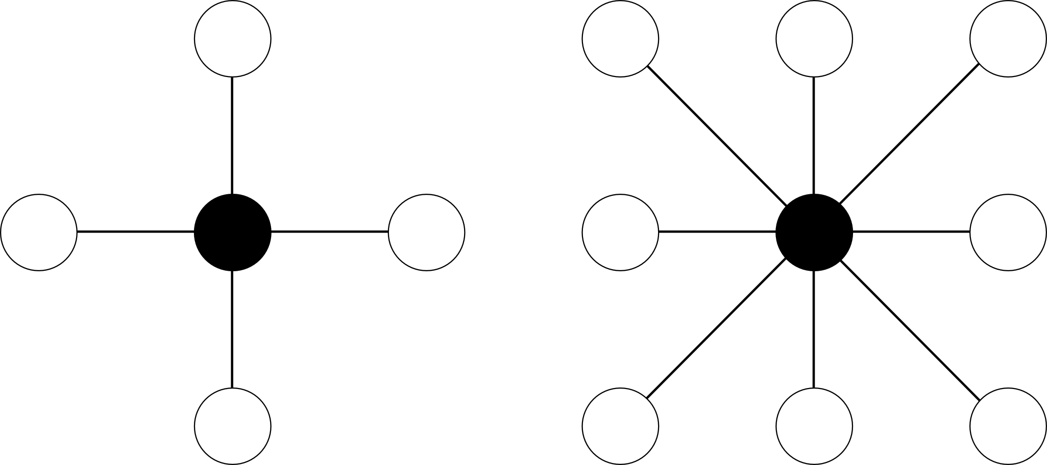
To describe spatial correlations between pixels, it is important to properly define a neighborhood structure. The neighborhood relation between two pixels and has to be symmetric: if is a neighbor of then is a neighbor of . This relation is applied to the nearest neighbors of the considered pixel, for example the fourth, eighth or twelfth nearest pixels. Fig. 1 shows two examples of neighborhood structures. The four pixel structure or -order neighborhood will be considered in the rest of the paper. Therefore, the associated set of neighbors, or cliques, has only vertical and horizontal possible configurations (see [Besag1974, Geman1984] for more details).
Once the neighborhood structure has been established, the MRF can be defined. Let denote a random variable associated to the th pixel of an image of pixels. In the context of hyperspectral image unmixing, the variables indicate the pixel classes and take their values in a finite set where is the number of possible classes. The whole set of random variables forms a random field. An MRF is then defined when the conditional distribution of given the other pixels only depend on its neighbors , i.e.,
| (4) |
where is the neighborhood structure considered and .
Since the pioneer work of Geman [Geman1984], MRFs have been widely used in the image processing community as in [Kevrann1995, Tonazzini2006]. The hyperspectral community has also recently exploited the advantages of MRFs for hyperspectral image analysis [Rand2003, Rellier2004, Bali2008]. However, to our knowledge, MRFs have not been studied for hyperspectral image unmixing. MRFs provide an efficient way of modeling correlations between pixels, which is adapted to the intrinsic properties of most images. Two specific MRFs are appropriate for image analysis: the Ising model for binary random variables and the Potts-Markov model that is a simple generalization to more-than-two variables [Wu1982]. This paper focuses on the Potts-Markov model since it is very appropriate to hyperspectral image segmentation [Bali2008]. Given a discrete random field attached to an image with pixels, the Hammersley-Clifford theorem yields
| (5) |
where is the granularity coefficient, is the normalizing constant or partition function [Kindermann1980] and is the Kronecker function
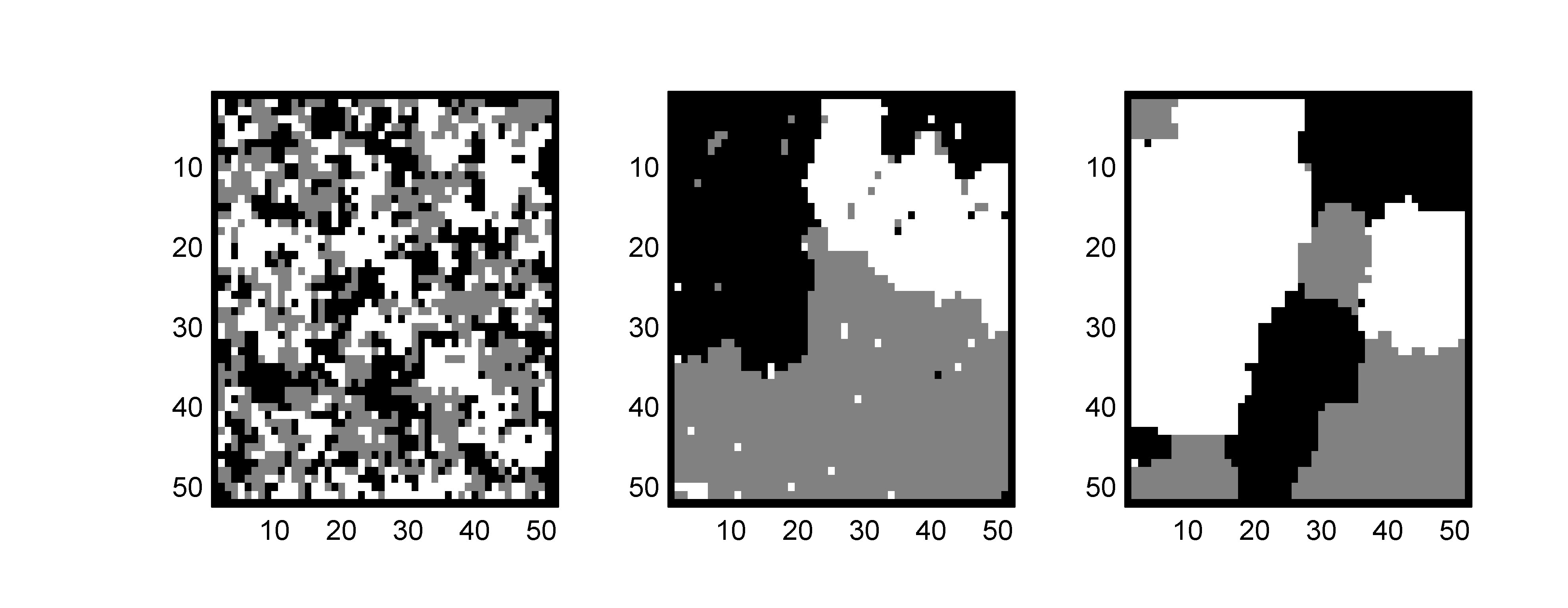
Note that drawing a label vector from the distribution (5) can be easily achieved without knowing by using a Gibbs sampler (the corresponding algorithmic scheme is summarized in [Eches2010_techreport_TGRS]). However, a major difficulty with the distribution (5) comes from the partition function that has no closed-form expression and depends on the unknown hyperparameter . The hyperparameter tunes the degree of homogeneity of each region in the image. Some simulations have been conducted to show the influence of this parameter on image homogeneity. Synthetic images have been generated from a Potts-Markov model with (corresponding to three gray levels in the image) and a -order neighborhood structure. Fig. 2 indicates that a small value of induces a noisy image with a large number of regions, contrary to a large value of that leads to few and large homogeneous regions. It is unnecessary to consider values of since for the -order neighborhood structure adopted here, “When , the Potts-Markov model is almost surely concentrated on single-color images” [Marin2007, p. 237]. Note however that for larger neighborhood systems, a smaller value of would be enough to obtain uniform patches in Potts realizations since, for example, is expected to be about twice for an -order neighborhood structure [Ripley1988]. In this work, the granularity coefficient will be fixed a priori. However, it is interesting to mention that the estimation of might also be conducted by using the methods studied in [Zhou1997], [Descombes1999] and [Celeux2003].
II-D Abundance Reparametrization
As explained before, the fraction vectors should satisfy positivity and sum-to-one constraints defined as
| (6) |
To ensure that these abundance constraints are satisfied, we have considered a reparametrization for positive parameters summing to one that was introduced in [Kent1988] for the spectral unmixing of satellite images. Note that this reparametrization has also shown interesting results for a pharmacokinetic problem [Gelman1996] and has been recently applied to hyperspectral unmixing [Themelis2008]. This reparametrization consists of rewriting the abundances as a function of random variables that will be referred to as logistic coefficients in the rest of the paper. A logistic coefficient vector is assigned to each abundance vector , according to the relationship
| (7) |
Initially, the spatial dependencies resulting from the image partitioning described in Section II-B are based on the first and second order moments of the abundance vectors . However, the spatial constraints defined in (3) can be easily adapted when using logistic coefficient vectors. Indeed, in each class, the unknown logistic coefficient vectors are assumed to share the same first and second order moments, i.e.,
| (8) |
With this reparametrization, the th class is fully characterized by the unknown hyperparameters and .
III Hierarchical Bayesian model
This section investigates the likelihood and the priors inherent to the LMM for the spectral unmixing of hyperspectral images, based on Potts-Markov random fields and logistic coefficients.
III-A Unknown parameters
The unknown parameter vector associated to to the LMM unmixing strategy is denoted as
where is the noise variance, is the label vector and with is the logistic coefficient matrix used for the abundance reparametrization. Note that the noise variance has been assumed to be unknown in the present paper, contrary to the model considered in [Kent1988].
III-B Likelihood
The additive white Gaussian noise sequence of the LMM allows one to write333Note that the dependence of the abundance vector on the logistic coefficient vector through (7) has been explicitly mentioned by denoting . (). Therefore the likelihood function of is
| (9) |
where means proportional to and is the standard norm. By assuming independence between the noise sequences (), the likelihood of the image pixels is
| (10) |
III-C Parameter priors
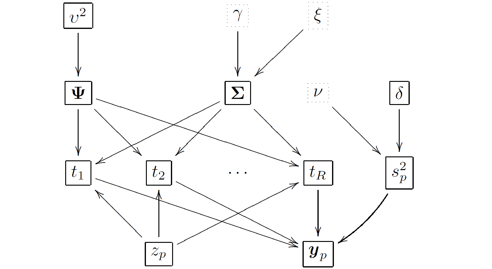
This section defines the prior distributions of the unknown parameters and their associated hyperparameters that will be used for the LMM. The directed acyclic graph (DAG) for the parameter priors and hyperpriors for the considered model is represented in Fig. 3.
III-C1 Label prior
The prior distribution for the label vector introduced in paragraph II-C is a Potts-Markov random field with a -order neighborhood and a known granularity coefficient (fixed a priori). The resulting prior distribution can be written as in (5) where is the -order neighborhood depicted in Fig. 1 (left).
III-C2 Logistic coefficient prior
Following the approach described in Section II-B, each component of is assumed to be distributed according to a Gaussian distribution. In addition, as highlighted in II-D (see (8)), the mean and variance of the logistic coefficients depend on the class to which the corresponding pixel belong. Therefore, the prior distribution for the is explicitly defined conditionally upon the pixel label
| (11) |
where the hyperparameters and depend on the associated pixel class . As suggested in Section I, a hierarchical Bayesian algorithm will be used to estimate these hyperparameters. For a given pixel , by assuming prior independence between the coefficients , the prior distribution for the vector is
| (12) |
where and is the diagonal matrix whose diagonal elements are .
By assuming prior independence between the vectors , the full posterior distribution for the logistic coefficient matrix is
| (13) |
with and .
III-C3 Noise variance prior
A conjugate inverse-gamma distribution is assigned to the noise variance
| (14) |
where and are adjustable hyperparameters. This paper assumes (as in [Punskaya2002] or [Tourneret2007]) and estimates jointly with the other unknown parameters and hyperparameters (using a hierarchical Bayesian algorithm).
III-D Hyperparameter priors
Hierarchical Bayesian algorithms require to define prior distributions for the hyperparameters. A particular attention has to be devoted to the hyperparameters and since they fully describe the different classes partitioning the image. The prior distributions for and are conjugate distributions. More precisely, a vague inverse-gamma distribution is chosen for the logistic coefficient variance , i.e.,
| (15) |
where and have been tuned to and (in order to obtain a large variance). Moreover, a centered Gaussian distribution with unknown variance has been chosen as prior for the logistic coefficient mean
| (16) |
where is another adjustable hyperparameter. By assuming independence between the different mean vectors , as well as between the covariance matrices for , the full priors for the two hyperparameters and can be expressed as
| (17) |
| (18) |
Jeffreys’ priors are chosen for the hyperparameters and (see, e.g., [Robert2007choice, p. 131] for details including computations)
| (19) |
where denotes the indicator function defined on . These choices, also adopted in [Punskaya2002, Dobigeon_IEEE_TSP_2007b], reflect the lack of knowledge regarding these two hyperparameters. At this last hierarchy level within the Bayesian inference, the hyperparameter vector can be defined as .
III-E Joint distribution
The joint posterior distribution of the unknown parameters and hyperparameters is classically defined using the hierarchical structure
| (20) |
Straightforward computations yield the following posterior
| (21) |
with . The posterior distribution (21) associated to the LMM is too complex to obtain closed-from expressions for the MMSE or MAP estimators of the unknown parameter vector . To alleviate this problem, we propose to use MCMC methods to generate samples that are asymptotically distributed according to (21). The generated samples are then used to approximate the Bayesian estimators. The next section studies a hybrid Gibbs sampler that generates samples asymptotically distributed according to the posterior distribution (21).
IV Hybrid Gibbs sampler
This section studies a Metropolis-within-Gibbs sampler that generates samples according to the joint posterior . The proposed sampler iteratively generates samples distributed according to the conditional distributions detailed below.
IV-A Conditional distribution of the label vector
For each pixel , the class label is a discrete random variable whose conditional distribution is fully characterized by the probabilities
| (22) |
where ( is the number of classes) and denotes the vector whose th element has been removed. These posterior probabilities can be expressed as
| (23) |
where . Note that the posterior probabilities of the label vector in (23) define an MRF. Consequently, sampling from this conditional distribution can be achieved using the scheme detailed in [Eches2010_techreport_TGRS], i.e., by drawing a discrete value in the finite set with the probabilities (23).
IV-B Conditional distribution of logistic coefficient matrix
For each pixel , the Bayes theorem yields
Straightforward computations lead to
| (24) |
Unfortunately, it is too difficult to generate samples distributed according to (24). Therefore, a Metropolis-Hastings step is used, based on a random walk method [Robert2004, p. 245] with a Gaussian distribution as proposal distribution. The variance of the instrumental distribution has been fixed to obtain an acceptance rate between and as recommended in [Roberts1996].
IV-C Conditional distributions of the noise variance
The Bayes theorem yields
As a consequence, is distributed according to the inverse-Gamma distribution
| (25) |
IV-D Conditional distribution of and
For each endmember () and each class (), the conditional distribution of can be written as
| (26) |
Similarly, the conditional distribution of is
| (27) |
Straightforward computations allow one to obtain the following results
| (28) |
| (29) |
with
IV-E Conditional distribution of and
The conditional distributions of and are the following inverse-gamma and gamma distributions, respectively
V Simulation results on synthetic data
| Actual values | Estimated values | ||
| Class | |||
| Class | |||
| Class | |||
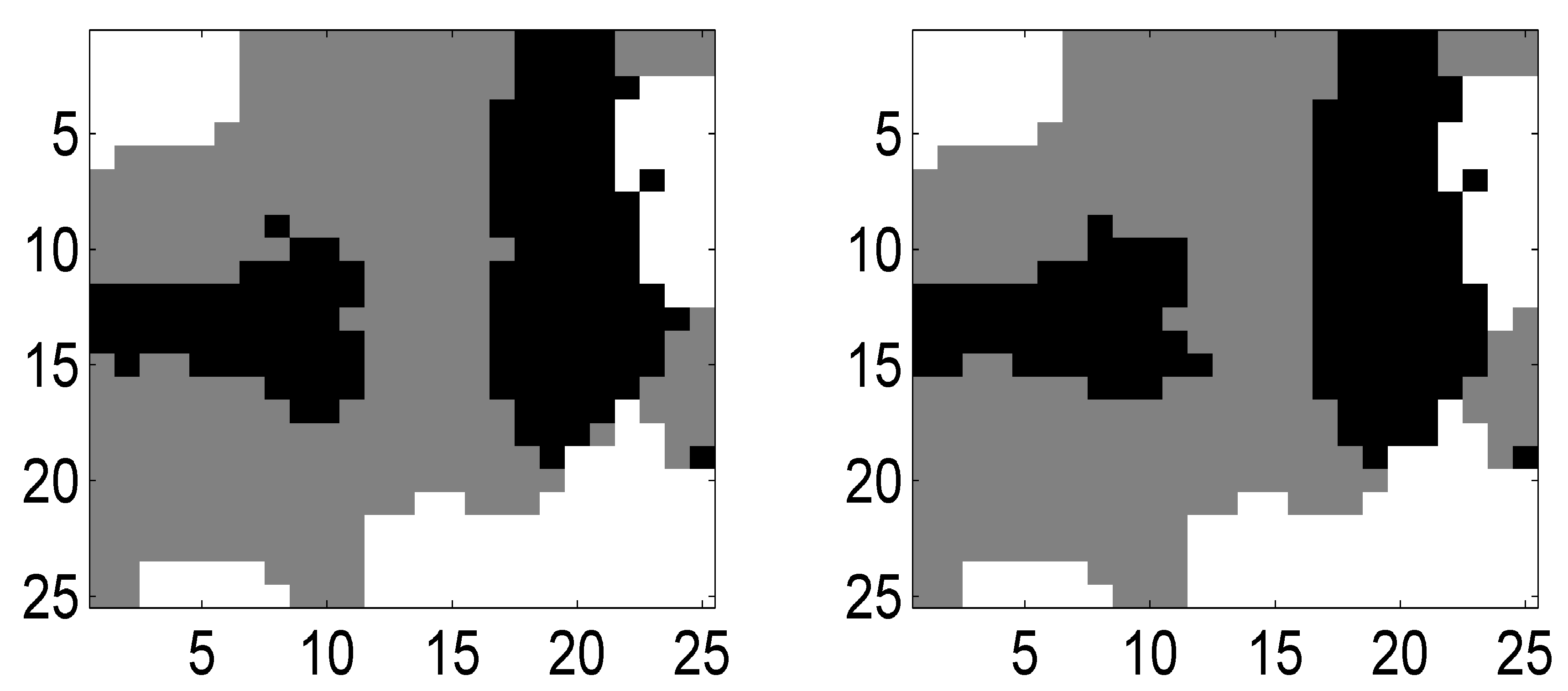
Many simulations have been conducted to illustrate the accuracy of the proposed algorithm. The first experiment considers a synthetic image with different classes. The image contains mixed components (construction concrete, green grass and micaceous loam) whose spectra ( spectral bands) have been extracted from the spectral libraries distributed with the ENVI package [ENVImanual2003]. A label map shown in Fig. 4 (left) has been generated using (5) with .
The mean and variance of the abundances have been chosen for each class as reported in Table I. These values reflect the fact that the st endmember is more present in Class (with average concentration of ), the nd endmember is more present in Class (with average concentration of ) and the rd endmember is more present in Class (with average concentration of ). In this simulation scenario, the abundance variance has been fixed to a common value for all endmembers, pixels and classes. The generated abundance maps for the LMM are depicted in Fig. 5. Note that a white (resp. black) pixel in the fraction map indicates a large (resp. small) value of the abundance coefficient. The noise variance is chosen such as the average signal-to-noise ratio (SNR) is equal to , i.e. .


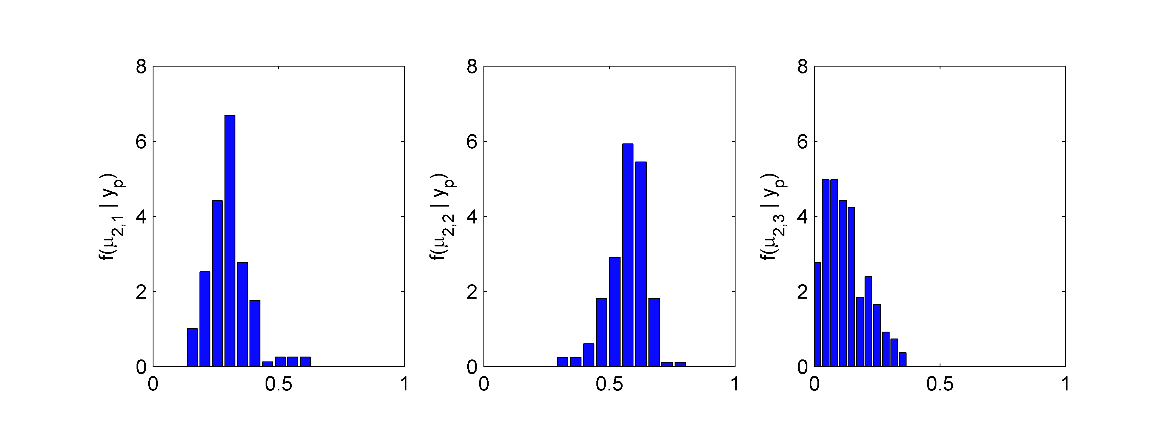
The MMSE and MAP estimators for the unknown parameters can be computed from samples generated with the Gibbs samplers presented in Section IV. For instance, the marginal MAP estimates of the label vector are depicted in Fig. 4 (right) for the proposed hybrid Gibbs algorithm. The MMSE estimates of the abundances conditioned upon are shown in Fig. 5. A number of iterations (including burn-in iterations) has been necessary to obtain these results. The proposed algorithm generates samples distributed according to the full posterior of interest. Then, these samples can be used to compute, for instance, the posterior distributions of the mean vectors (, ). These mean vectors, introduced in (3), are of great interest since they characterize each class. Therefore, as an additional insight, the histograms of the abundance means estimated by the proposed algorithm have been depicted in Fig. 6 for the nd class, i.e., . Similar results have been obtained for the other classes. They are omitted here for brevity. Finally, the estimated abundance means and variances have been reported in Table I (last row). The estimated classes, abundance coefficients and abundance mean vectors are clearly in accordance with their actual values.
The LMM hybrid Gibbs algorithm is compared respectively with its non-spatial constrained Bayesian counterpart developed in [Dobigeon_IEEE_TSP_2008]. The synthetic image shown in Fig. 4 has been analyzed by the initial algorithm of [Dobigeon_IEEE_TSP_2008] with the same number of iterations in addition with the FCLS [Heinz2001] algorithm. As a criterion, the global mean square error (MSE) of the th estimated abundances have been computed for each algorithm. This global MSE is defined as
| (30) |
where denotes the MMSE estimate of the abundance . Table II reports the different results showing that the algorithm developed in this paper (referred to as “Spatial”) performs better than the non-spatial constrained algorithms (referred to as “Bayesian” and “FCLS”).
| FCLS | Bayesian | Spatial | |
|---|---|---|---|
VI Simulation results on AVIRIS Images
VI-A Performance of the proposed algorithm
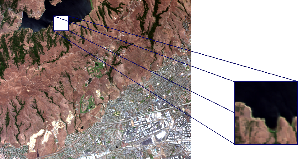
This section illustrates the performance of the proposed spatial algorithm on a real hyperspectral dataset, acquired over Moffett Field (CA, USA) in by the JPL spectro-imager AVIRIS. Many previous works have used this image to illustrate and compare algorithm performance with hyperspectral images [Christophe2005, Akgun2005]. The first region of interest, represented in Fig. 7, is a image. The data set has been reduced from the original bands to bands by removing water absorption bands. As in [Dobigeon_IEEE_TSP_2008], a principal component analysis has been conducted as a processing step to determine the number of endmembers present in the scene. Then, the endmembers spectra have been extracted with the help of the endmember extraction procedure N-FINDR proposed by Winter in [Winter1999]. The extracted endmembers, shown in Fig. 8, corresponds to soil, vegetation and water444Note that the influence of the endmember extraction step on the unmixing results has been investigated in [Eches2010_techreport_TGRS] by coupling the proposed algorithm with other EEAs.. The algorithm proposed in Section IV has been applied on this image with iterations (with burn-in iterations). The number of classes has been fixed to since prior knowledge on the scene allows one to identify areas in the image: water point, lake shore, vegetation and soil.

The estimated classification and abundance maps for the proposed hybrid Gibbs algorithm are depicted in Fig. 9 (left) and 10 (top). The results provided by the algorithm are very similar and in good agreement with results obtained on this image with an LMM-based Bayesian algorithm [Dobigeon_IEEE_TSP_2008] (Fig. 10, middle) or with the well-known FCLS algorithm [Heinz2001] (Fig. 10, bottom).


The performance of the proposed algorithm has been also evaluated for different values of the number of endmembers . The resulting classification maps for and are given in Fig. 9 (middle and right). These maps show that the classification results are quite robust with respect to the number of endmembers. The corresponding abundance maps can be found in [Eches2010_techreport_TGRS], as well as the results of the proposed algorithm when the number of classes vary.
The computational time of the proposed method (combined with the N-FINDR procedure) has been compared with the computational times of two other unmixing algorithms when applied on this Moffett image: the FCLS algorithm (also combined with N-FINDR) and the constrained nonnegative matrix factorization (cNMF) algorithm that jointly estimates the endmember matrix and the abundances [Sajda2004]. The results555These simulations have been carried out with an unoptimized MATLAB b bit implementation on a Core(TM)Duo GHz computer. are reported in Table III. The proposed method (referred to as “Spatial”) has the higher computational cost when compared to the two others, mainly due to the joint estimation of the labels and the abundance vectors. However, it provides more information about unmixing. In particular, the samples generated with the proposed Gibbs sampler can be used to determine confidence intervals for the estimated parameters.
| FCLS | cNMF | Spatial | |
|---|---|---|---|
| Times (s.) |
VI-B Simulation on a larger image
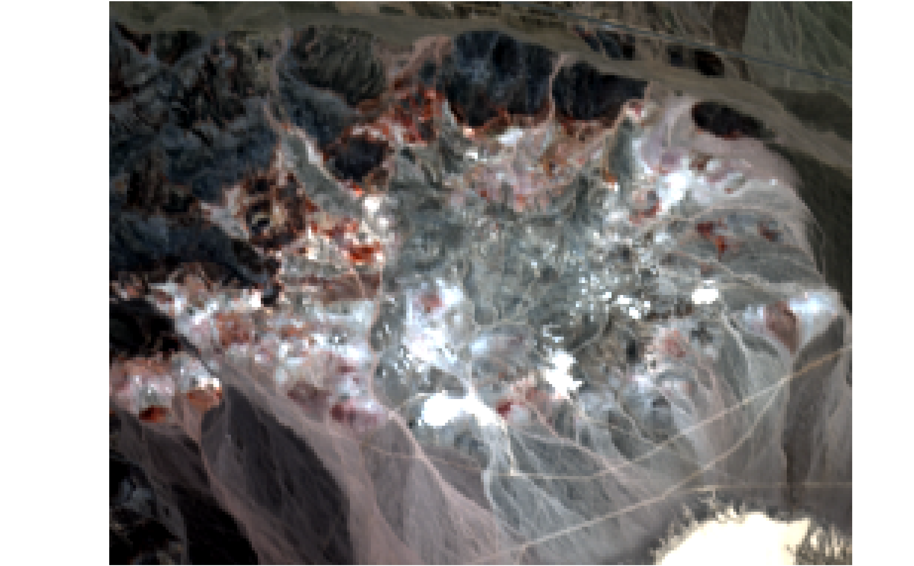
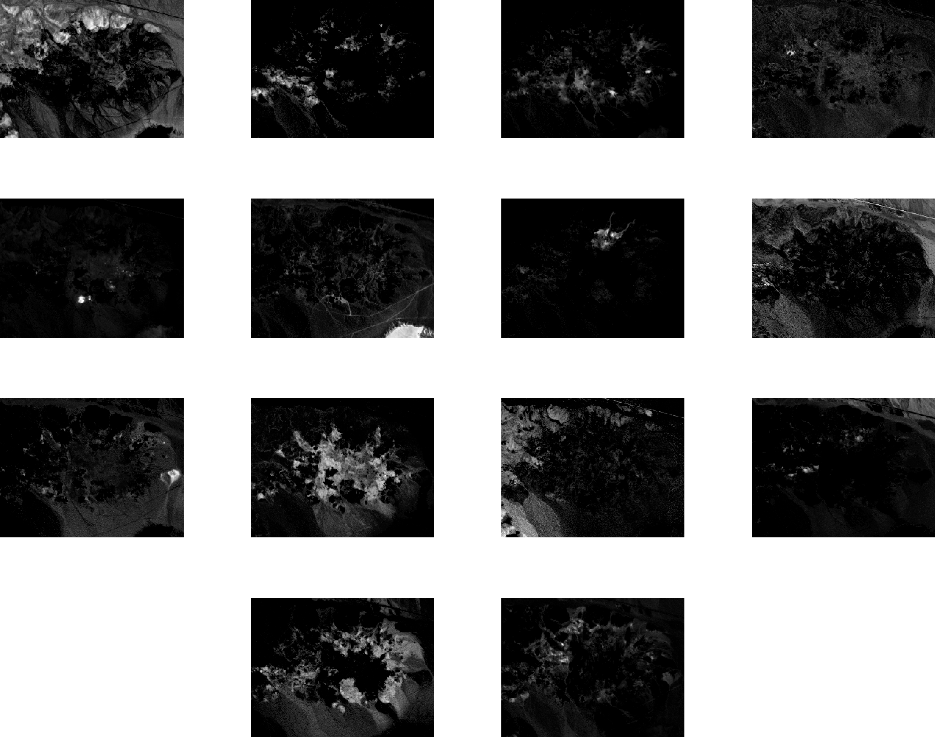
The performance of the proposed Bayesian algorithm has also been evaluated on a larger real hyperspectral image. The selected scene has been extracted from the AVIRIS Cuprite image, acquired over a mining site in Nevada, in . The geologic characteristics of the complete data have been mapped in [Clark1993, Clark2003]. The area of interest of size is represented in Fig. 11 and has been previously studied in [Nascimento2005] to test the VCA algorithm with . Therefore, in this experiment, the same number of endmembers has been extracted by the VCA algorithm. The number of classes has been set to , which seems to be a sufficient value to capture the natural diversity of the scene. The proposed algorithm has been used to estimate the abundance and label maps related to the analyzed scene. These maps are depicted in Fig. 12 and 14, respectively.
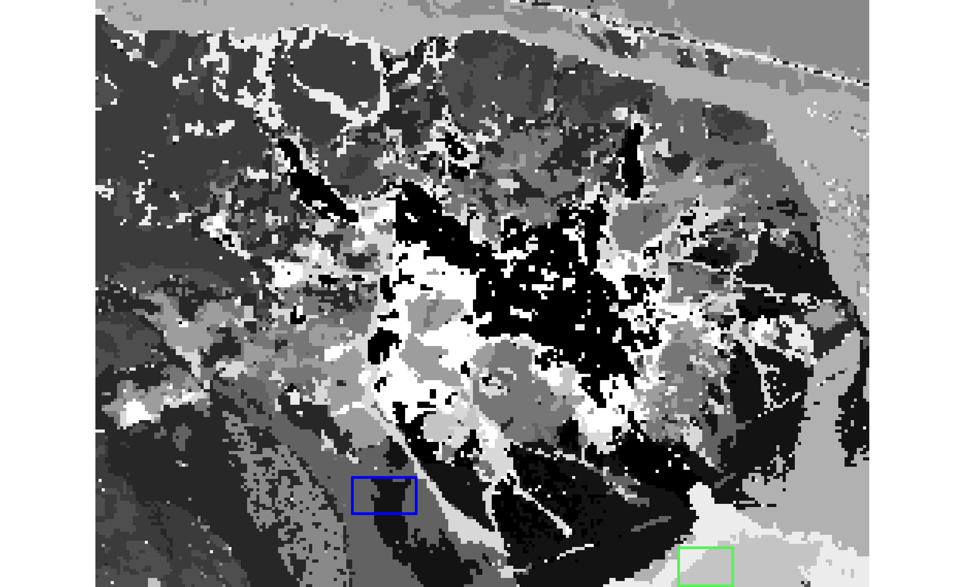
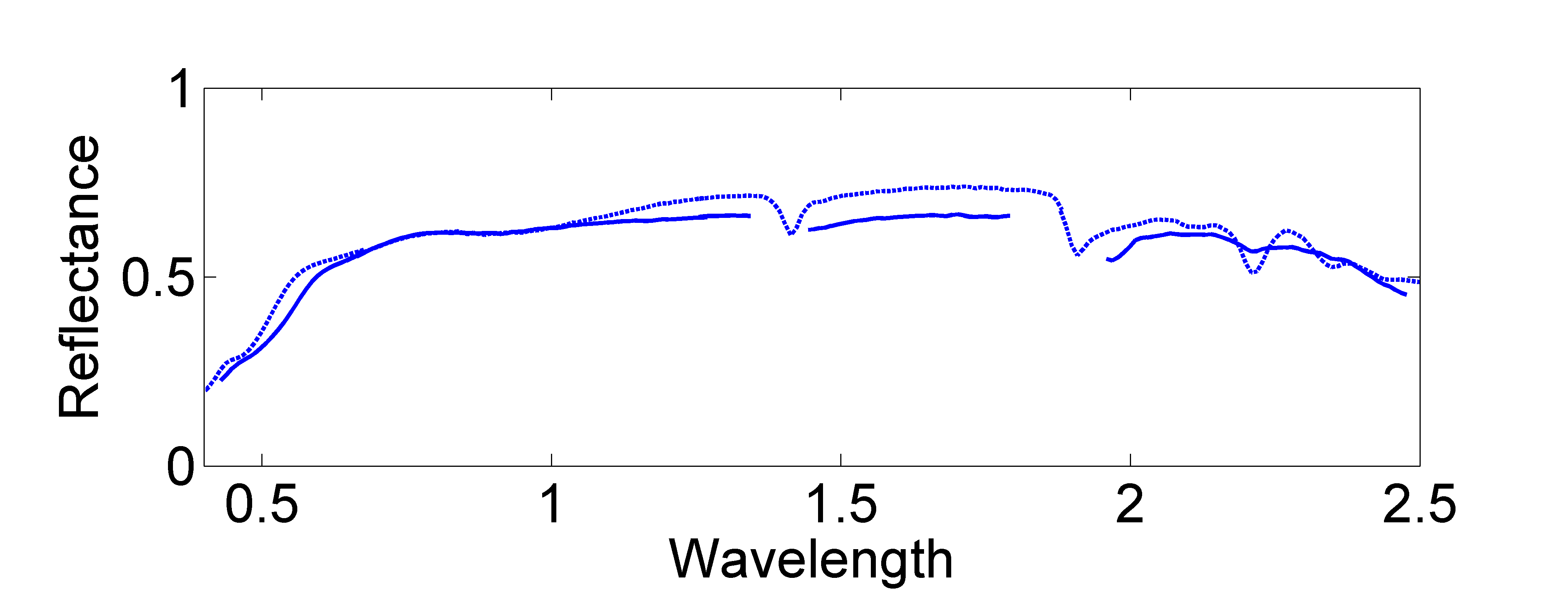
The proposed Bayesian inversion algorithm has been able to identify some regions similar to those recovered in [Nascimento2005]. To illustrate, the composition of two particular areas (marked as colored rectangles in Fig. 12) is investigated. Tables IV report the abundance means for the most significant endmembers that appear in the two highlighted regions. From these tables, one can conclude that the two classes represented in black and dark gray of the “blue” area are composed of very mixed pixels (the abundance of the most significant endmember is ). On the other hand, both classes in the “green” area are clearly dominated by the th endmember. By comparing its corresponding signature with the materials included in the USGS library spectra, this th endmember matches the Montmorillonite spectrum (see Fig. 13). This result is in good agreement with the ground truth. Indeed, from [Clark2003], Montmorillonnite is the most commonly found material in this area.
| Green area | ||
|---|---|---|
| light gray | white | |
| Endm. | ||
| Endm. | ||
| Endm. | ||
| Endm. | ||
| Blue area | ||
|---|---|---|
| black | dark gray | |
| Endm. | ||
| Endm. | ||
| Endm. | ||
| Endm. | ||
VII Conclusions
A new hierarchical Bayesian algorithm was proposed for hyperspectral image unmixing. Markov random fields were introduced to model spatial correlations between the pixels of the image. A hidden discrete label was introduced for each pixel of the image to identify several classes defined by homogeneous abundances (with constant first and second order statistical moments). The positivity and sum-to-one constraints on the abundances were handled by using an appropriate reparametrization defined by logistic coefficient vectors. We derived the joint posterior distribution of the unknown parameters and hyperparameters associated to the proposed Bayesian linear mixing model. An MCMC method was then studied to generate samples asymptotically distributed according to this posterior. The generated samples were then used to estimate the abundance maps as well as the underlying image labels. The results obtained on simulated data and on real AVIRIS images are very promising. Future works include the estimation of the granularity coefficient involved in Potts-Markov random fields.
Acknowledgments
The authors would like to thank one of the reviewers for pointing out the relevant paper [Kent1988] and for his valuable suggestions that helped to improve the manuscript.