A Markov Chain Approximation of a Segment Description of Chaos

Abstract.

We test a Markov chain approximation to the segment description (Li, 2007) of chaos (and turbulence) on a tent map, the Minea system, the Hénon map, and the Lorenz system. For the tent map, we compute the probability transition matrix of the Markov chain on the segments for segment time length (iterations) $T=1,2,3,100$. The matrix has $1,2,4$ tents corresponding to $T=1,2,3$; and is almost uniform for $T=100$. As $T\rightarrow+\infty$, our conjecture is that the matrix will approach a uniform matrix (i.e. every entry is the same). For the simple fixed point attractor in the Minea system, the Reynolds average performs excellently and better than the maximal probability Markov chain and segment linking. But for the strange attractors in the Hénon map, and the Lorenz system, the Reynolds average performs very poorly and worse than the maximal probability Markov chain and segment linking.

1. Markov Chain Approximation

In [3], we showed that any orbit inside an attractor (chaotic or turbulent attractors are the most interesting ones) can be uniformly approximated on the infinite time interval $t\in[0,\infty)$ by an infinite sequence of segments out of a finite number of segments. The attractor (or its attracting neighborhood) is partitioned into $N$ small neighborhoods $\{A_{n}\}_{n=1,2,\cdots,N}$. Each neighborhood $A_{n}$ is attached with an orbit segment $s_{n}$ over a fixed time interval $t\in[0,T]$. Denote by $F^{t}$ the evolution operator. The flow tube $\cup_{t\in[0,T]}F^{t}(A_{n})$ is approximated by the segment $s_{n}$. If $F^{T}(A_{n})\cap A_{m}\neq\emptyset$, then the flow tube $\cup_{t\in[T,2T]}F^{t}(F^{T}(A_{n})\cap A_{m})$ is approximated by the segment $s_{m}$. This process can be continued to $t\rightarrow\infty$. If we re-distribute the Lebesgue measure of $F^{T}(A_{n})\cap A_{m}$ uniformly on $A_{m}$ (i.e. we assume the points in $F^{T}(A_{n})\cap A_{m}$ as random points with uniform probability distribution in $A_{m}$), then we obtain a Markov chain approximation. When $A_{n}$’s are small and the attractor has good mixing properties, we expect this Markov chain approximation to perform very well. The key element for this Markov chain approximation is the transition matrix [2], [1]

(1) $$\Lambda=\left(\rho_{ij}\right)\ ,$$

where

$$\rho_{ij}=\frac{\mu(F^{T}(A_{j})\cap A_{i})}{\mu(F^{T}(A_{j}))}\ ,$$

and $\mu$ is the Lebesgue measure. We can simply label $A_{n}$ and $s_{n}$ by the letter $n$. Then our Markov chain is defined by the transition matrix $\Lambda$ acting on $N$ letters $\{1,2,\cdots,N\}$.

2. Ulam Approximation

The Transfer Operator (Perron-Frobenius Operator) is defined as,

(2) $$\nu_{n+1}(A)=\nu_{n}(F^{-T}(A))=\sum_{j=1}^{N}\nu_{n}(F^{-T}(A)\cap A_{j})\ ,$$

where $\nu_{n}$’s are measures. The Ulam approximation of the transfer operator is defined as,

(3) $$\nu_{n+1}(A)=\sum_{j=1}^{N}\frac{\mu(F^{-T}(A)\cap A_{j})}{\mu(A_{j})}\nu_{n}(A_{j})\ ,$$

where $\mu$ is the Lebesgue measure. If we re-distribute $\nu_{n}(F^{-T}(A)\cap A_{j})$ uniformly on $A_{j}$ (i.e. we assume the points in $F^{T}(A)\cap A_{j}$ as random points with uniform probability distribution in $A_{j}$), then we obtain the Ulam approximation by

$$\nu_{n}(F^{-T}(A)\cap A_{j})\sim\frac{\mu(F^{-T}(A)\cap A_{j})}{\mu(A_{j})}\nu_{n}(A_{j})\ .$$

The transition matrix of the Ulam approximation is

(4) $$P=\left(\sigma_{ij}\right)\ ,$$

where

$$\sigma_{ij}=\frac{\mu(F^{-T}(A_{i})\cap A_{j})}{\mu(A_{j})}\ .$$

If $F^{T}$ is $1-1$ and we replace the partition $\{A_{i}\}$ by $\{F^{T}(A_{i})\}$, then

$$\sigma_{ij}=\frac{\mu(A_{i}\cap F^{T}(A_{j}))}{\mu(F^{T}(A_{j}))}=\rho_{ij}\ .$$

3. Asymptotic Cycles

Using the segments $\{s_{n}\}_{n=1,2,\cdots,N}$, one can identify certain pseudo-orbits (called segment linking orbits) and the associated sequence of $A_{n}$’s:

$$\cdots s_{n_{-2}}s_{n_{-1}}s_{n_{0}}s_{n_{1}}s_{n_{2}}\cdots$$

$$\cdots A_{n_{-2}}A_{n_{-1}}A_{n_{0}}A_{n_{1}}A_{n_{2}}\cdots$$

where $s_{n_{j}}$ attaches to $A_{n_{j}}$ and the end point of $s_{n_{j}}$ belongs to $A_{n_{j+1}}$ (recall also that the starting point of $s_{n_{j}}$ belongs to $A_{n_{j}}$). Since there are only finite $s_{n}$’s; as $n_{j}\rightarrow+\infty$, some $s_{n_{j}}$ has to repeat itself, then all the segments after it repeat themselves too. Thus all these pseudo-orbits are always asymptotic to cycles:

$$\cdots\cdots s_{n_{j_{1}}}\cdots s_{n_{j_{k}}}s_{n_{j_{1}}}\cdots s_{n_{j_{k}}}\cdots$$

where $k$ can be $1$ in which case the asymptotic cycle is a “fixed point”.

4. Transition Matrix

We shall compute the transition matrix for the tent map:

$$x_{n+1}=f(x_{n}),\ x_{n}\in[0,1];$$

where

$$f(x_{n})=\frac{x_{n}}{a}\ (x_{n}<a),\ f(x_{n})=\frac{x_{n}-1}{a-1}\ (x_{n}\geq a);$$

and $a$ is a parameter $a\in(0,1)$. We choose $a=1/3$. We break the interval $[0,1]$ into $20$ subintervals. Take $100$ initial conditions in each subinterval. For each initial condition $x_{0}$ in the $i$-th subinterval, we compute $x_{T}$ as the $T$-iteration starting from $x_{0}$. If $x_{T}$ belongs to $j$-th subinterval, we increase the $(j,i)$-th entry of the transition matrix by $\frac{1}{100}$. Initially all the entries of the transition matrix are set to $0$. Since the iterated map $f^{T}$ has $2^{T-1}$ tents, the transition matrix also resembles this pattern. Our conjecture is that when $T\rightarrow+\infty$, the transition matrix approaches a uniform matrix with every entry being $1/20$. See Figure 1 for an illustration.

5. Different Types of Orbits

We shall compute several types of orbits:

1. The true orbit. It is computed by Runge-Kutta method for differential equations, and by iterations for maps; for a time interval $t\in[0,T^{*}]$.

2. The segment orbit. First we cut the total time interval $[0,T^{*}]$ into subintervals of length $T$. The interested region in the phase space, where the attractor lives is partitioned into $N$ small neighborhood $\{A_{n}\}_{n=1,2,\cdots,N}$ (usually squares or cubes). If at time $t=jT$, the true orbit lands in some $A_{n}$, then $(j+1)$-th segment will be the one attached to $A_{n}$ (usually this segment is computed with the initial condition at the center of the square or cube for a time length of $T$). For $j=0,1,2,\cdots$; all the segments together form the segment orbit. It is a uniform approximation of the true orbit for all positive time.

3. The segment linking orbit. If the initial condition of the true orbit lands in some $A_{n}$, then the first segment will be the one attached to $A_{n}$. If the first segment ends in some $A_{m}$, then the second segment will be the one attached to $A_{m}$. By repeating this process, we generate the segment linking orbit. As discussed in Section 3, the segment linking orbit is asymptotic to some cycle. The segment orbit uniformly approximates a particular orbit in the basin of attraction, while the segment linking orbit only uses the initial condition of the true orbit, and is not a uniform approximation of the true orbit. In reality, the segment orbit is difficult to obtain without the full knowledge of the true orbit, while the segment linking orbit is trivial to obtain once all the segments attached to the $A_{n}$’s are known.

4. The maximal probability Markov chain. If the initial condition of the true orbit lands in some $A_{n}$, then the first segment will be the one attached to $A_{n}$. Then we test many random initial points in $A_{n}$, see where they land at time $t=T$, and we pick maximal probability partition element $A_{m}$. The second segment will be the one attached to $A_{m}$. Repeating the process, we generate the maximal probability Markov chain.

5. The Reynolds average orbit. We pick initial conditions near the initial condition of the true orbit, compute the orbit corresponding to each initial condition, at each $t\geq 0$, we do an algebraic average of all the orbits, then we get the Reynolds average orbit.

Overall, the segment orbit is a uniform approximation of a particular orbit, while the segment linking orbit, the maximal probability Markov chain and the Reynolds average orbit are all aiming at certain average property of the attractor.

6. Minea System

Consider the Minea system

$$\frac{du_{1}}{dt} = 1-u_{1}-\delta u_{2}^{2}\ ,$$

$$\frac{du_{2}}{dt} = \delta u_{1}u_{2}-u_{2}\ ;$$

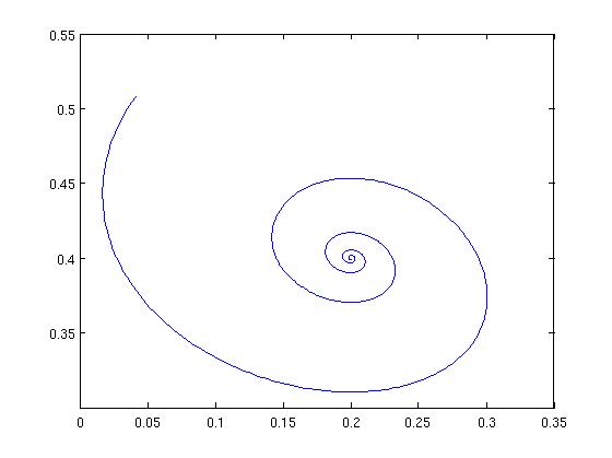
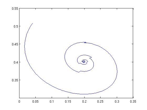
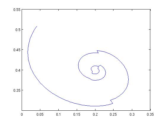
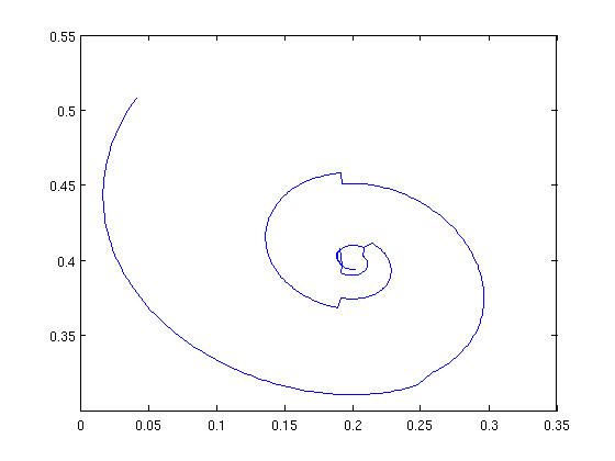
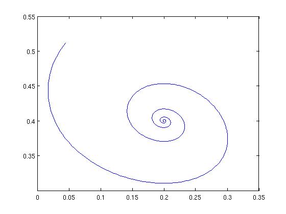
where $(u_{1},u_{2})\in(0,1)\times(0,1)$ and $\delta$ is a parameter. When $\delta>1$, all the orbits converge to one point [6]. We choose $\delta=5$ for our simulations here. The total simulation time $T^{*}=10$, while the segment time $T=1$ (i.e. $10$ segments along each orbit). The interested region in the phase plane is $(u_{1},u_{2})\in(0,1)\times(0,1)$. We cut this unit square into $60\times 60$ subsquares (i.e. the $A_{n}$’s). The segment attached to each $A_{n}$ starts from the center of $A_{n}$. The true orbit starts from the initial point ($\frac{1}{24},0.5+\frac{1}{120}$). For the calculation of the maximal probability Markov chain, we test $1000$ random initial points in $A_{n}$. For the calculation of the Reynolds average orbit, we pick $4$ initial conditions within $\frac{1}{120}$ distance from the initial condition of the true orbit. The results are shown in Figure 2. As expected, the Reynolds average orbit is a better approximation of the true orbit than the other types of orbits.

7. Hénon Map

Consider the Hénon map

$$x_{n+1} = y_{n}+1-1.4x_{n}^{2},$$

$$y_{n+1} = 0.3x_{n}.$$

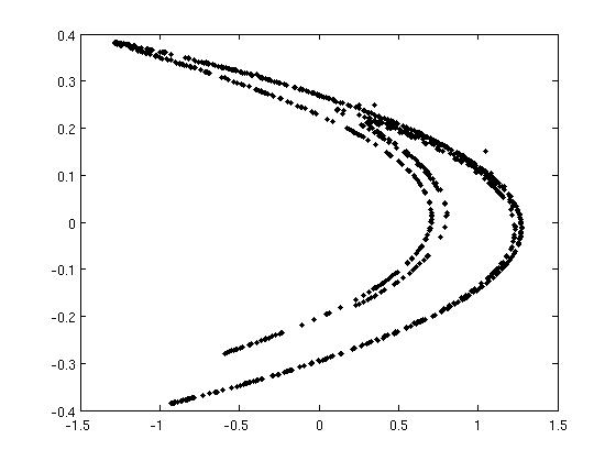
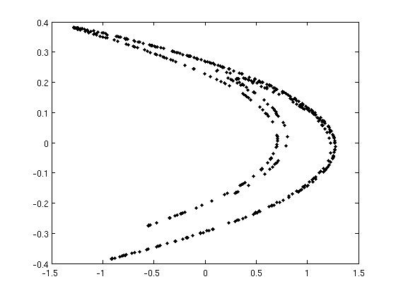
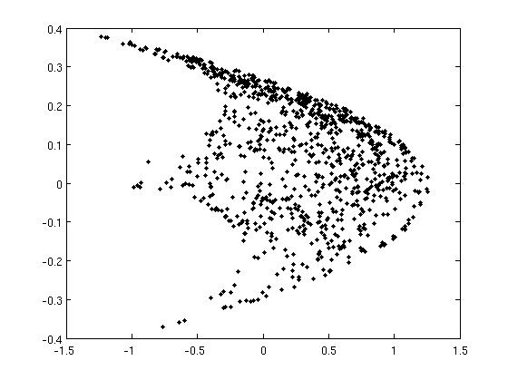
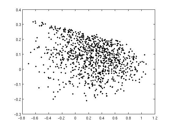
The total simulation time $T^{*}=1000$ (iterations), while the segment time $T=250$ (i.e. $4$ segments along each orbit). The interested region in the phase plane is $(x_{n},y_{n})\in(-2,2)\times(-2,2)$. We cut this square into $40\times 40$ subsquares (i.e. the $A_{n}$’s). The segments attached to each $A_{n}$ starts from the center of $A_{n}$. The true orbit starts from the initial point ($0.631354477,0.189406343$). For the calculation of the maximal probability Markov chain, we test $1000$ random initial points in $A_{n}$. For the calculation of the Reynolds average orbit, we pick $2$ or $4$ initial conditions within $10^{-6}$ distance from the initial condition of the true orbit. The results are shown in Figure 3. One thing is clear, that is, the Reynolds average orbits are definitely bad approximations to the true orbit, and bad descriptions of the strange attractor.

8. Lorenz System

Consider the Lorenz system

$$\frac{dx}{dt} = a(y-x),$$

$$\frac{dy}{dt} = x(b-25z)-y,$$

$$\frac{dz}{dt} = 25xy-cz,$$

where we choose $a=10$, $b=28$, $c=8/3$.

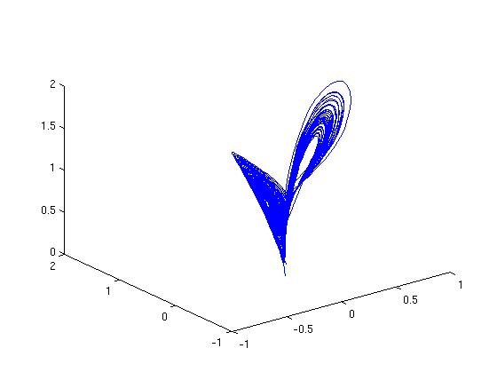
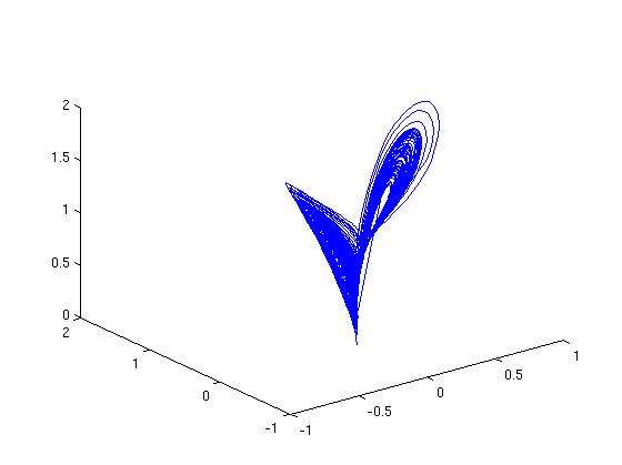
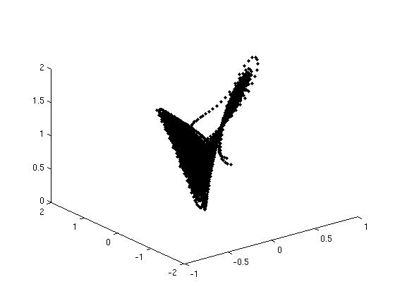
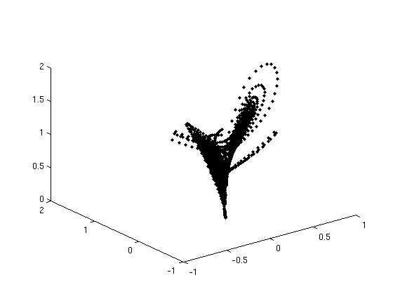
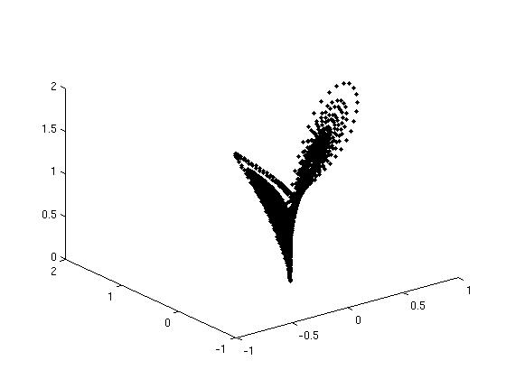
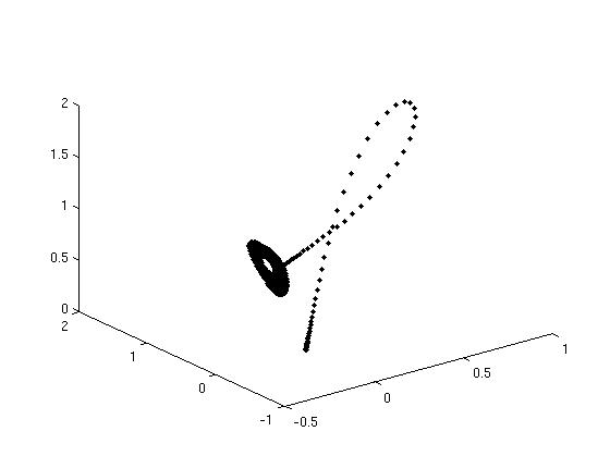
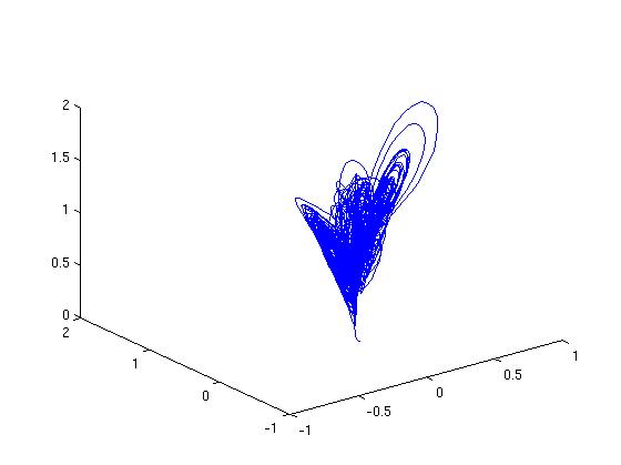
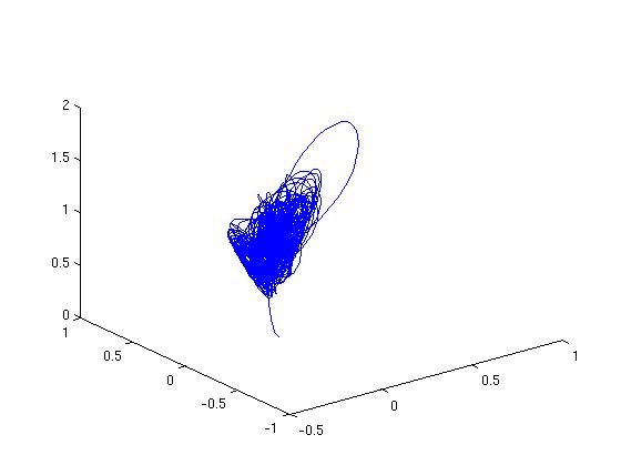
The total simulation time $T^{*}=100$, while the segment time is either $T=10$ (i.e. $10$ segments along each orbit) or $T=1$ (i.e. $100$ segments along each orbit). The interested region in the phase space is $(x,y,z)\in(-0.8,0.8)\times(-1,1)\times(0,2)$. We cut this region into $16\times 16\times 16$ subregions (i.e. the $A_{n}$’s). The segments attached to each $A_{n}$ starts from the center of $A_{n}$. The true orbit starts from the initial point ($0.1,0,0$). For the calculation of the maximal probability Markov chain, we test $1000$ random initial points in $A_{n}$. For the calculation of the Reynolds average orbit, we pick $2$ or $4$ initial conditions within $0.05$ distance from the initial condition of the true orbit. The results are shown in Figures 4 and 5. Once again the Reynolds average orbits are definitely bad approximations to the true orbit, and bad descriptions of the strange attractor. Naturally as the number of the segments along an orbit increases, the segment linking orbit and the maximal probability Markov chain deviate further away from the true orbit.

9. Conclusion and Discussion

As discussed in details in [3] [4] [5], an effective description of turbulence means a solution to the problem of turbulence. An effective description of chaos is also very useful in applications of chaos theory.

It is dangerous to draw strong conclusion with limited numerical experiments. But it is clear from these numerical experiments here that the Reynolds average is a terrible description of strange attractors. The segment description has the potential to generate useful descriptions of strange attractors. Both the segment linking and the Markov chain have the potential to generate useful characterizations on certain average properties of the strange attractors.

Traditionally the Reynolds average is based upon the setup of typical orbits being high frequency oscillations around a mean orbit. This is not the case inside a strange attractor. Therefore, one should not expect that the Reynolds average can be a good description on any sort of average property of the strange attractor. For the segment description, computing the segments can be costly if the partition is fine enough. Computing the segment orbit associated with a true orbit needs the full knowledge of the true orbit. So the potential of the segment description lies at the statistics of the segments rather than any individual segment orbit. Segment linking is a convenient way to start the study on the statistics of the segments. Markov chain is a first level study on the statistics of the segments. Practically it is very costly to generate the probability transition matrix for the Markov chain.

Finally what kind of average properties that a strange attractor may possess are not clear at all. If the strange attractor has ergodicity, then tracking one orbit is enough to get a good picture of the strange attractor. On the other hand, especially in higher dimensions, often the chaotic (turbulent) dynamics is transient. What kind of average properties that such transient dynamics may possess are even less clear.

(a) $T=1$

(b) $T=2$

(c) $T=3$

(d) $T=100$

Figure 1. Transition matrices for the tent map

(a) true orbit

(b) segment orbit

(c) segment linking orbit

(d) maximal probability Markov chain

(e) Reynolds average orbit

Figure 2. Different types of orbits for the Minea system.

(a) true orbit

(b) segment orbit

(c) segment linking orbit

(d) maximal probability Markov chain

(e) Reynolds average orbit (of 2 orbits)

(f) Reynolds average orbit (of 4 orbits)

Figure 3. Different types of orbits for the Hénon map.

(a) true orbit

(b) segment orbit (10)

(c) segment orbit (100)

(d) segment linking orbit (10)

(e) segment linking orbit (100)

Figure 4. Different types of orbits for the Lorenz system (part 1).

(a) maximal probability Markov chain (10)

(b) maximal probability Markov chain (100)

(c) Reynolds average orbit (of 2 orbits)

(d) Reynolds average orbit (of 4 orbits)

Figure 5. Different types of orbits for the Lorenz system (part 2).

References

- [1] J. Ding, T.-Y. Li, A. Zhou, Finite approximations of Markov operators, Journal of Computational and Applied Mathematics 147 (2002), 137-152.
- [2] J. Kemeny, J. Snell, Finite Markov Chain, D. Van Nostrand Company, Inc. Princeton, New Jersey, 1960.
- [3] Y. Li, Segment description of turbulence, Dynamics of PDE 4, no.3 (2007), 283-291.
- [4] Y. Li, Chaos in partial differential equations, Navier-Stokes equations and turbulence, Proceedings of the 4th International Congress of Chinese Mathematicians, (Hangzhou, December 17-22, 2007), vol. III, 110-122, Higher Education Press, Beijing, China
- [5] Y. Li, On the true nature of turbulence,The Mathematical Intelligencer 29, no.1 (2007), 45-48.
- [6] R. Temam, Infinite-dimensional Dynamical Systems in Mechanics and Physics, Springer-Verlag, 1988.