Soccer: is scoring goals a predictable Poissonian process?

Abstract

The non-scientific event of a soccer match is analysed on a strictly scientific level. The analysis is based on the recently introduced concept of a team fitness (Eur. Phys. J. B 67, 445, 2009) and requires the use of finite-size scaling. A uniquely defined function is derived which quantitatively predicts the expected average outcome of a soccer match in terms of the fitness of both teams. It is checked whether temporary fitness fluctuations of a team hamper the predictability of a soccer match. To a very good approximation scoring goals during a match can be characterized as independent Poissonian processes with pre-determined expectation values. Minor correlations give rise to an increase of the number of draws. The non-Poissonian overall goal distribution is just a consequence of the fitness distribution among different teams. The limits of predictability of soccer matches are quantified. Our model-free classification of the underlying ingredients determining the outcome of soccer matches can be generalized to different types of sports events.

In recent years different approaches, originating from the physics community, have shed new light on sports events, e.g. by studying the behavior of spectators Farkas et al. (2002), by elucidating the statistical vs. systematic features behind league tables Ben-Naim et al. (2007); Ben-Naim and Hengartner (2007); Wesson (2002), by studying the temporal sequence of ball movements Mendes et al. (2007) or using extreme value statistics Gembris et al. (2002); Greenhough et al. (2002) known, e.g., from finance analysis Mantegna and Stanley (1995). For the specific case of soccer matches different models have been introduced on phenomenological grounds Lee (1997); Dixon and Coles (1997); Dixon and Robinson (1998); Rue and Salvesen (2000); Koning (2000); Dobson and Goddard (2003). However, very basic questions related, e.g., to the relevance of systematic vs. statistical contributions or the temporal fitness evolution are still open. It is known that the distribution of soccer goals is broader than a Poissonian distribution Greenhough et al. (2002); Bittner et al. (2007, 2009). This observation has been attributed to the presence of self-affirmative effects during a soccer matchBittner et al. (2007, 2009), i.e. an increased probability to score a goal depending on the number of goals already scored by that team.

In this work we introduce a general model-free approach which allows us to elucidate the outcome of sports events. Combining strict mathematical reasoning, appropriate finite-size scaling and comparison with actual data all ingredients of this framework can be quantified for the specific example of soccer. A unique relation can be derived to calculate the expected outcome of a soccer match and three hierarchical levels of statistical influence can be identified. As one application we show that the skewness of the distribution of soccer goals Greenhough et al. (2002); Bittner et al. (2007, 2009) can be fully related to fitness variations among different teams and does not require the presence of self-affirmative effects.

As data basis we take all matches in the German Bundesliga (www.bundesliga-statistik.de) between seasons 1987/88 and 2007/08 except for the year 1991/92 (in that year the league contained 20 teams). Every team plays 34 matches per season. Earlier seasons are not taken into account because the underlying statistical properties (in particular number of goals per match) are somewhat different.

Conceptually, our analysis relies on recent observations in describing soccer leagues Heuer and Rubner (2009): (i) The home advantage is characterized by a team-independent but season-dependent increase of the home team goal difference $c_{home}>0$. (ii) An appropriate observable to characterize the fitness of a team $i$ in a given season is the average goal difference (normalized per match) $\Delta G_{i}(N)$, i.e. the difference of the goals scored and conceded during $N$ matches. In particular it contains more information about the team fitness than, e.g., the number of points.

Figure 1: The correlation function $h(t)$. The average value of $h(t)$ is included (excluding the value for $t=17$) yielding approx. $0.22$ Heuer and Rubner (2009).

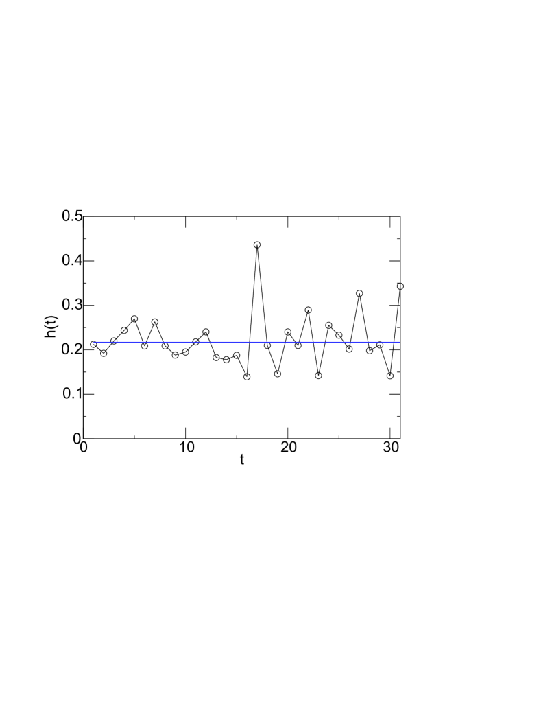
Straightforward information about the team behavior during a season can be extracted from correlating its match results from different match days. Formally, this is expressed by the correlation function $h(t)=\langle\Delta g_{ij}(t_{0})\Delta g_{ik}(t_{0}+t)\rangle$. Here $\Delta g_{ij}:=g_{i}-g_{j}$ denotes the goal difference of a match of team $i$ vs. team $j$ with the final result $g_{i}:g_{j}$. $j$ and $k$ are the opponents of team $i$ at match days $t_{0}$ and $t_{0}+t$. The home-away asymmetry can be taken into account by the transformation $\Delta g_{ij}\rightarrow\Delta g_{ij}\mp c_{home}$ where the sign depends on whether team $i$ plays at home or away. The resulting function $h(t)$ is shown in Fig.1. Apart from the data point for $t=17$ one observes a time-independent positive plateau value. The absolute value of this constant corresponds to the variance $\sigma_{\Delta G}^{2}$ of $\Delta G_{i}$ and is thus a measure for the fitness variation in a league Heuer and Rubner (2009). Furthermore, the lack of any decay shows that the fitness of a team is constant during the whole season. This result is fully consistent with the finite-size scaling analysis in Ref.Heuer and Rubner (2009) where additionally the fitness change between two seasons was quantified. The exception for $t=17$ just reflects the fact that team $i$ is playing against the same team at days $t_{0}$ and $t_{0}+17$, yielding additional correlations between the outcome of both matches (see also below).

As an immediate consequence, the limit of $\Delta G_{i}(N)$ for large $N$, corresponding to the true fitness $\Delta G_{i}$, is well-defined. A consistent estimator for $\Delta G_{i}$, based on the information from a finite number of matches, reads

$$\Delta G_{i}=a_{N}\Delta G_{i}(N).$$ (1)

with $a_{N}\approx 1/[1+3/(N\sigma^{2}_{\Delta G})]$ Heuer and Rubner (2009) . For large $N$ the factor $a_{N}$ approaches unity and the estimation becomes error-free, i.e. $\Delta G_{i}(N)\rightarrow\Delta G_{i}$. For $N=33$ one has $a_{N}=0.71$ and the variance of the estimation error is given by $\sigma_{e,N}^{2}=(N/3+1/\sigma_{\Delta G}^{2})^{-1}\approx 0.06$ Heuer and Rubner (2009). This statistical framework is known as regression toward the mean Stigler (2002). Analogously, introducing $\Sigma G_{i}(N)$ as the average sum of goals scored and conceded by team $i$ in $N$ matches its long-time limit is estimated via $\Sigma G_{i}-\lambda=b_{N}(\Sigma G_{i}(N)-\lambda)$ where $\lambda$ is the average number of goals per match in the respective season. Using $\sigma^{2}_{\Sigma G}\approx 0.035$ one correspondingly obtains $b_{N=33}=0.28$ Heuer and Rubner (2009).

Our key goal is to find a sound characterization of the match result when team $i$ is playing vs. team $j$, i.e. $\Delta g_{ij}$ or even $g_{i}$ and $g_{j}$ individually. The final outcome $\Delta g_{ij}$ has three conceptually different and uncorrelated contributions

$$\Delta g_{ij}=q_{ij}+f_{ij}+r_{ij}.$$ (2)

Averaging over all matches one can define the respective variances $\sigma_{q}^{2},\sigma_{f}^{2}$ and $\sigma_{r}^{2}$. (1) $q_{ij}$ expresses the average outcome which can be expected based on knowledge of the team fitness values $\Delta G_{i}$ and $\Delta G_{j}$, respectively. Conceptually this can be determined by averaging over all matches when teams with these fitness values play against each other. The task is to determine the dependence of $q_{ij}\equiv q(\Delta G_{i},\Delta G_{j})$ on $\Delta G_{i}$ and $\Delta G_{j}$. (2) For a specific match, however, the outcome can be systematically influenced by different factors beyond the general fitness values using the variable $f_{ij}$ with a mean of zero: (a) External effects such as several players which are injured or tired, weather conditions (helping one team more than the other), or red cards. As a consequence the effective fitness of a team relevant for this match may differ from the estimation $\Delta G_{i}$ (or $\Delta G_{j}$). (b) Intra-match effects depending on the actual course of a match. One example is the suggested presence of self-affirmative effects, i.e. an increased probability to score a goal (equivalently an increased fitness) depending on the number of goals already scored by that team Bittner et al. (2007, 2009). Naturally, $f_{ij}$ is much harder to predict if possible at all. Here we restrict ourselves to the estimation of its relevance via determination of $\sigma_{f}^{2}$. (3) Finally, one has to understand the emergence of the actual goal distribution based on expectation values as expressed by the random variable $r_{ij}$ with average zero. This problem is similar to the physical problem when a decay rate (here corresponding to $q_{ij}+f_{ij}$) has to be translated into the actual number of decay processes.

Determination of $q_{ij}$: $q_{ij}$ has to fulfill the two basic conditions (taking into account the home advantage): $q_{ij}-c_{home}=-(q_{ji}-c_{home})$ (symmetry condition) and $\langle q_{ij}\rangle_{j}-c_{home}=\Delta G_{i}$ (consistency condition) where the average is over all teams $j\neq i$ (in the second condition a minor correction due to the finite number of teams in a league is neglected). The most general dependence on $\Delta G_{i,j}$ up to third order, which is compatible with both conditions, is given by

$$q_{ij}=c_{home}+(\Delta G_{i}-\Delta G_{j})\cdot[1-c_{3}(\sigma^{2}_{\Delta G}+\Delta G_{i}\Delta G_{j})].$$ (3)

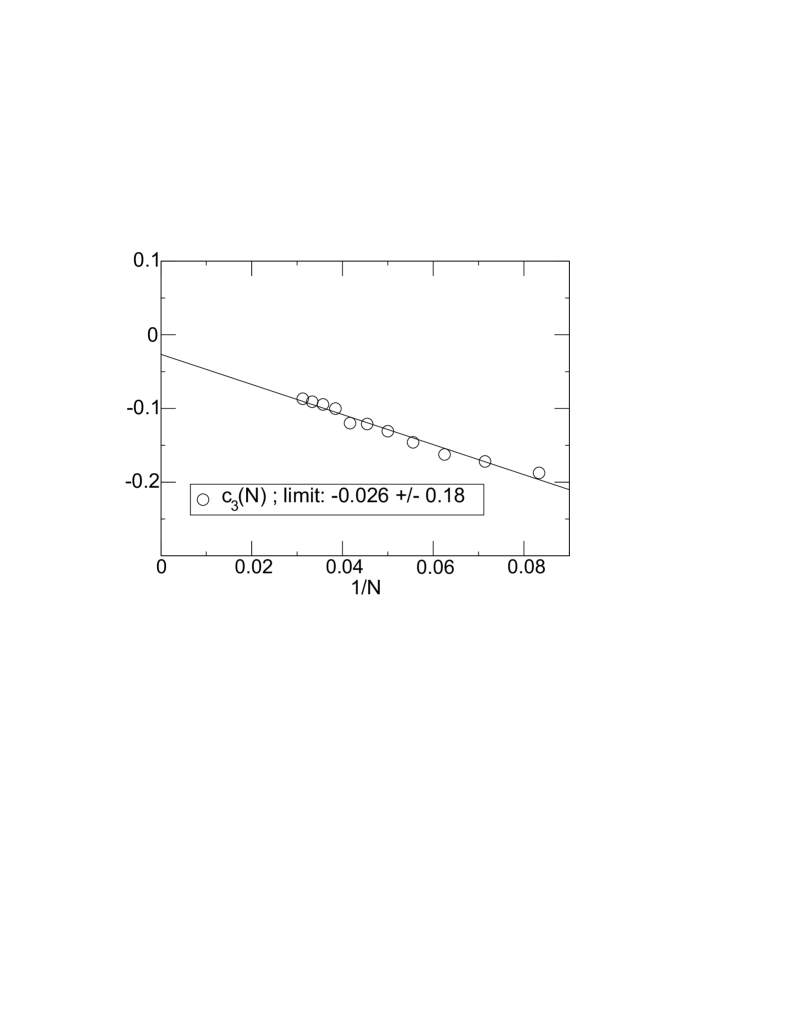
Qualitatively, the $c_{3}$-term takes into account the possible effect that in case of very different team strengths (e.g. $\Delta G_{i}\gg 0$ and $\Delta G_{j}\ll 0$) the expected goal difference is even more pronounced ($c_{3}>0$: too much respect of the weaker team) or reduced ($c_{3}<0$: tendency of presumption of the better team). On a phenomenological level this effect is already considered in the model of, e.g., Ref.Rue and Salvesen (2000). The task is to determine the adjustable parameter $c_{3}$ from comparison with actual data. We first rewrite Eq.3 as $q_{ij}-(\Delta G_{i}-\Delta G_{j})-c_{home}=-c_{3}(\Delta G_{i}-\Delta G_{j})(\sigma^{2}_{\Delta G}+\Delta G_{i}\Delta G_{j})$. In case that $\Delta G_{i,j}$ is known this would correspond to a straightforward regression problem of $\Delta g_{ij}-(\Delta G_{i}-\Delta G_{j})-c_{home}$ vs. $-(\Delta G_{i}-\Delta G_{j})(\sigma^{2}_{\Delta G}+\Delta G_{i}\Delta G_{j})$. An optimum estimation of the fitness values for a specific match via Eq.1 is based on $\Delta G_{i,j}(N)$, calculated from the remaining $N=33$ matches of both teams in that season . Of course, the resulting value of $c_{3}(N=33)$ is still hampered by finite-size effects, in analogy to the regression towards the mean. This problem can be solved by estimating $c_{3}(N)$ for different values of $N$ and subsequent extrapolation to infinite $N$ in an $1/N$-representation. Then our estimation of $c_{3}$ is not hampered by the uncertainty in the determination of $\Delta G_{i,j}$. For a fixed $N\leq 30$ the regression analysis is based on 50 different choices of $\Delta G_{i,j}(N)$ by choosing different subsets of $N$ matches to improve the statistics. The result is shown in Fig.2. The estimated error results from performing this analysis individually for each season. Due to the strong correlations for different $N$-values the final error is much larger than suggested by the fluctuations among different data points. The data are compatible with $c_{3}=0$. Thus, we have shown that the simple choice

$$q_{ij}=\Delta G_{i}-\Delta G_{j}+c_{home}$$ (4)

is the uniquely defined relation (neglecting irrelevant terms of 5th order) to characterize the average outcome of a soccer match. In practice the right side can be estimated via Eq.1. This result implies that $h(t)=\langle(\Delta G_{i}-\Delta G_{j})(\Delta G_{i}-\Delta G_{k})\rangle=\sigma_{\Delta G}^{2}+\langle\Delta G_{j}\Delta G_{k}\rangle$, i.e. $h(t\neq 17)=\sigma_{\Delta G}^{2}$ and $h(t=17)=2\sigma_{\Delta G}^{2}$. This agrees very well with the data. Furthermore, the variance of the $q_{ij}$ distribution, i.e. $\sigma_{q}^{2}$, is by definition given by $2\sigma_{\Delta G}^{2}\approx 0.44$.

Figure 2: Determination of $c_{3}$ by finite-size scaling.

Determination of $\sigma_{f}^{2}$: This above analysis does not contain any information about the match-specific fitness relative to $\Delta G_{i}-\Delta G_{j}$. For example $f_{ij}>0$ during a specific match implies that team $i$ plays better than expected from $q_{ij}$. The conceptual problem is to disentangle the possible influence of these fitness fluctuations from the random aspects of a soccer match. The key idea is based on the observation that, e.g., for $f_{ij}>0$ team $i$ will play better than expected in both the first and the second half of the match. In contrast, the random features of a match do not show this correlation. For the identification of $\sigma_{f}^{2}$ one defines $A=\langle((\Delta g^{(1)}_{ij}/b_{1}-c_{home})\cdot((\Delta g^{(2)}_{ij}/b_{2}-c_{home})\rangle_{ij}$ where $\Delta g^{(1),(2)}_{ij}$ is the goal difference in the first and second half in the specific match, respectively and $b_{1,2}$ the fraction of goals scored during the first and the second half, respectively ($b_{1}=0.45;b_{2}=0.55$). Based on Eq.4 one has $\sigma_{f}^{2}=A-2\sigma_{\Delta G}^{2}$. Actually, to improve the statistics we have additionally used different partitions of the match (e.g. first and third quarter vs. second and fourth quarter). Numerical evaluation yields $\sigma_{f}^{2}=-0.04\pm 0.06$ where the error bar is estimated from individual averaging over the different seasons. Thus one obtains in particular $\sigma_{f}^{2}\ll\sigma^{2}_{q}$ which renders match-specific fitness fluctuations irrelevant. Actually, as shown in Heuer and Rubner (2009), one can observe a tendency that teams which have lost 4 times in a row tend to play worse in the near future than expected by their fitness. Strictly speaking these strikes indeed reflect minor temporary fitness variations. However, the number of strikes is very small (less than 10 per season) and, furthermore, mostly of statistical nature. The same holds for red cards which naturally influence the fitness but fortunately are quite rate. Thus, these extreme events are interesting in their own right but are not relevant for the overall statistical description. The negative value of $\sigma_{f}^{2}$ points towards anti-correlations between both partitions of the match. A possible reason is the observed tendency towards a draw, as outlined below.

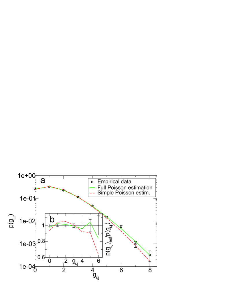
Figure 3: (a)Distribution of goals per team and match and the Poisson prediction if the different fitness values are taken into account (solid line). Furthermore a Poisson estimation is included where only the home-away asymmetry is included (broken line). The quality of the predicted distribution is highlighted in (b) where the ratio of the estimated and the actual probability is shown.

Determination of $r_{ij}$: The actual number of goals $g_{i,j}$ per team and match is shown in Fig.3. The error bars are estimated based on binomial statistics. As discussed before the distribution is significantly broader than a Poisson distribution, even if separately taken for the home and away goals Greenhough et al. (2002); Bittner et al. (2007, 2009). Here we show that this distribution can be generated by assuming that scoring goals are independent Poissonian processes. We proceed in two steps. First, we use Eq.4 to estimate the average goal difference for a specific match with fitness values estimated from the remaining 33 matches of each team. Second, we supplement Eq.4 by the corresponding estimator for the sum of the goals $g_{i}+g_{j}$ given by $\Sigma G_{i}+\Sigma G_{j}-\lambda$. Together with Eq.4 this allows us to calculate the expected number of goals for both teams individually. Third, we generate for both teams a Poissonian distribution based on the corresponding expectation values. The resulting distribution is also shown in Fig.1 and perfectly agrees with the actual data up to 8 (!) goals. In contrast, if the distribution of fitness values is not taken into account significant deviations are present. Two conclusions can be drawn. First, scoring goals is a highly random process. Second, the good agreement again reflects the fact that $\sigma_{f}^{2}$ is small because otherwise an additionally broadening of the actual data would be expected. Thus there is no indication of a possible influence of self-affirmative effects during a soccer match Bittner et al. (2007, 2009). Because of the underlying Poissonian process the value of $\sigma_{r}^{2}$ is just given by the average number of goals per match $(\approx 3)$.

Figure 4: (a) The probability distribution of the goal difference per match together with its estimation based on independent Poisson processes of both teams. In (b) it is shown for different scores how the ratio of the estimated and the actual number of draws differ from unity.

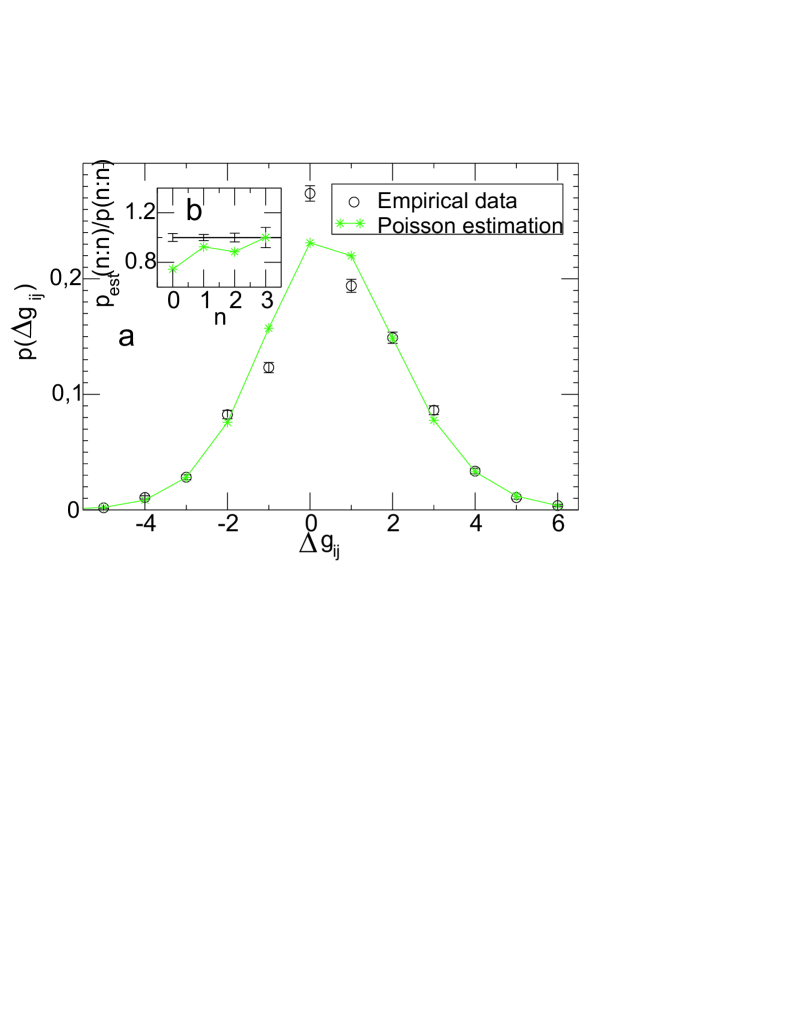
As already discussed in literature the number of draws is somewhat larger than expected on the basis of independent Poisson distributions; see, e.g., Refs. Dixon and Coles (1997); Rue and Salvesen (2000). As an application of the present results we quantify this statement. In Fig.4 we compare the calculated distribution of $\Delta g_{ij}$ with the actual values. The agreement is very good except for $\Delta g_{ij}=-1,0,1$. Thus, the simple picture of independent goals of the home and the away team is slightly invalidated. The larger number of draws is balanced by a reduction of the number of matches with exactly one goal difference. More specifically, we have calculated the relative increase of draws for the different results. The main effect is due to the strong increase of more than 20% of the 0:0 draws. Note that the present analysis has already taken into account the fitness distribution for the estimation of this number. Starting from 3:3 the simple picture of independent home and away goals holds again.

The three major contributions to the final soccer result display a clear hierarchy, i.e. $\sigma_{r}^{2}:\sigma_{q}^{2}:\sigma_{f}^{2}\approx 10^{2}:10^{1}:10^{0}$. $\sigma_{f}^{2}$, albeit well defined and quantifiable, can be neglected for two reasons. First, it is small as compared to the fitness variation among different teams. Second, the uncertainty in the prediction of $q_{ij}$ is, even at the end of the season, significantly larger (variance of the uncertainty: $2\cdot\sigma_{e,N=33}^{2}=0.12$, see above). Thus, the limit of predictability of a soccer match is, beyond the random effects, mainly related to the uncertainty in the fitness determination rather than to match specific effects. Thus, the hypothesis of a strictly constant team fitness during a season, even on a single-match level cannot be refuted even for a data set comprising more than 20 years. In disagreement with this observation soccer reports in media often stress that a team played particularly good or bad. Our results suggest that there exists a strong tendency to relate the assessment too much to the final result thereby ignoring the large amount of random aspects of a match.

In summary, apart from the minor correlations with respect to the number of draws soccer is a surprisingly simple match in statistical terms. Neglecting the minor differences between a Poissonian and binomial distribution and the slight tendency towards a draw a soccer match is equivalent to two teams throwing a dice. The number 6 means goal and the number of attempts of both teams is fixed already at the beginning of the match, reflecting their respective fitness in that season.

More generally speaking, our approach may serve as a general framework to classify different types of sports in a three-dimensional parameter space, expressed by $\sigma_{r}^{2},\sigma_{q}^{2},\sigma_{f}^{2}$. This set of numbers, e.g., determines the degree of competitiveness Ben-Naim and Hengartner (2007). For example for matches between just two persons (e.g. tennis) one would expect that fitness fluctuations ($\sigma_{f}^{2}$) play a much a bigger role and that for sports events with many goals or points (e.g. basketball) the random effects ($\sigma_{r}^{2}$) are much less pronounced, i.e. it is more likely that the stronger team indeed wins. Hopefully, the present work stimulates activities to characterize different types of sports along these lines.

We greatly acknowledge helpful discussions with B. Strauss, M. Trede, and M. Tolan about this topic.

References

- Farkas et al. (2002) I. Farkas, D. Helbing, and T. Vicsek, Nature 419, 131 (2002).
- Ben-Naim et al. (2007) E. Ben-Naim, S. Redner, and F. Vazquez, Europhys. Lett. 77, 30005/1 (2007).
- Ben-Naim and Hengartner (2007) E. Ben-Naim and N. W. Hengartner, Phys. Rev. E 76, 026106/1 (2007).
- Wesson (2002) J. Wesson, The Science of Soccer (Institute of Physics Publishing, 2002).
- Mendes et al. (2007) R. Mendes, L. Malacarne, and C. Anteneodo, Eur. Phys. J. B 57, 357 (2007).
- Gembris et al. (2002) D. Gembris, J. Taylor, and D. Suter, Nature 417, 506 (2002).
- Greenhough et al. (2002) J. Greenhough, P. Birch, S. Chapman, and G. Rowlands, Physica A 316, 615 (2002).
- Mantegna and Stanley (1995) R. Mantegna and H. Stanley, Nature 376, 46 (1995).
- Lee (1997) A. Lee, Chance 10, 15 (1997).
- Dixon and Coles (1997) M. Dixon and S. Coles, Appl. Statist. 46, 265 (1997).
- Dixon and Robinson (1998) M. Dixon and M. Robinson, The Statistician 47, 523 (1998).
- Rue and Salvesen (2000) H. Rue and O. Salvesen, The Statistician 49, 399 (2000).
- Koning (2000) R. Koning, The Statistician 49, 419 (2000).
- Dobson and Goddard (2003) S. Dobson and J. Goddard, European Journal of Operational Research 148, 247 (2003).
- Bittner et al. (2007) E. Bittner, A. Nussbaumer, W. Janke, and M. Weigel, Europhys. Lett. 78, 58002/1 (2007).
- Bittner et al. (2009) E. Bittner, A. Nussbaumer, W. Janke, and M. Weigel, Eur. Phys. J. B 67, 459 (2009).
- Heuer and Rubner (2009) A. Heuer and O. Rubner, Eur. Phys. J. B 67, 445 (2009).
- Stigler (2002) S. Stigler, Statistics on the Table. The History of Statistical Concepts and Methods. (Harvard University Press, 2002).