On the Shear Instability in Relativistic Neutron Stars
Abstract
We present new results on instabilities in rapidly and differentially rotating neutron stars. We model the stars in full general relativity and describe the stellar matter adopting a cold realistic equation of state based on the unified SLy prescription [1]. We provide evidence that rapidly and differentially rotating stars that are below the expected threshold for the dynamical bar-mode instability, , do nevertheless develop a shear instability on a dynamical timescale and for a wide range of values of . This class of instability, which has so far been found only for small values of and with very small growth rates, is therefore more generic than previously found and potentially more effective in producing strong sources of gravitational waves. Overall, our findings support the phenomenological predictions made by Watts, Andersson and Jones [2] on the nature of the low- instability as the manifestation of a shear instability in a region where the latter is possible only for small values of the . Furthermore, our results provide additional insight on shear instabilities and on the necessary conditions for their development.
pacs:
04.40.Dg, 95.30.Lz, 95.30.Sf 97.60.Jd1 Introduction
Non-axisymmetric deformations of rapidly rotating bodies are rather generic phenomena in Nature and can appear in a wide class of systems. Particularly interesting within an astrophysical context are those deformations taking place in fluids that are self-gravitating and the literature on this has a long history dating back to the work of [3] on incompressible Newtonian uniformly rotating bodies. Since then, the study of these instabilities has continued over the years both in Newtonian gravity and in full general relativity.
Special attention has traditionally been paid to the study of instabilities, which are characterized by the exponential growth of deformations, where parametrizes the azimuthal dependence in a standard mode decomposition in spherical harmonics. Most of the interest in this type of deformation in compact stars stems from the fact that it has the shortest growth time and leads to the emission of a strong gravitational-wave signal.
The development of non-axisymmetric instabilities is commonly analyzed in terms of the quantity (i.e. the ratio between the kinetic rotational energy and the gravitational potential energy ), that provides a dimensionless measure of the amount of angular momentum that can be tapped to feed the development of the instabilities. This parameter plays an important role in what is possibly the most celebrated of the non-axisymmetric instabilities: the so-called dynamical bar-mode instability. This is an instability which takes place when the parameter is larger than a critical one, . In the case of a Newtonian incompressible self-gravitating polytrope, for instance, the dynamical bar-mode instability develops for [3] and is only weakly dependent on the considered polytropic index or whether the fluid is compressible. Post-Newtonian (PN) studies [4] or fully general-relativistic ones [5] correct this results only slightly, by reducing the threshold to somewhat lower values of the instability parameter. As an example, for a polytropic relativistic star with polytropic index , the accurate calculations reported in [6] reveal that the critical value is and that a simple dependence on the stellar compactness allows one to track this threshold from the Newtonian limit over to the fully relativistic one [7].
The onset and development of the bar-mode instability has been traditionally studied by means of nonlinear 3D simulations of Newtonian stars that are either unmagnetized [8, 9, 10, 11, 12] and, more recently, also magnetized [13]. In addition, PN and fully relativistic simulations have been performed and highlighted, for instance, that the persistence of the bar is strongly dependent on the degree of overcriticality and is generically of the order of the dynamical timescale. Furthermore, generic nonlinear mode-coupling effects between the and the mode appear during the development of the instability and these can severely limit the persistence of the bar deformation and eventually suppress the bar deformation [6]. These results have been recently confirmed by the perturbative calculations in [14].
Besides dynamical instabilities, which are purely hydrodynamical, secular instabilities are also possible in rotating compact stars and these are instead triggered by dissipative processes, such as viscosity or radiation emission. If, in particular, the dissipative mechanism is the emission of gravitational radiation, then the secular instability is also known as Chandrasekhar-Friedman-Schutz or CFS instability [15, 16]. Contrary to what their name may suggest, secular instabilities do not necessarily develop on secular timescales (although they normally do) and are characterized by having a much smaller threshold for the instability. Once again, in the case of a Newtonian polytrope, the critical secular instability parameter is as small as and thus much more easy to attain in astrophysical circumstances.
Although widely observed in numerical simulations, the physical conditions leading to a dynamical bar-mode instability are difficult to be encountered in standard astrophysical scenarios. Such large values of the instability parameter, in fact, cannot be easily attained in old and cold neutron stars, which have been brought into uniform rotation and thus to rather small values of . However, more recently these pessimistic prospects have been changed when a new instability has been discovered in differentially rotating Newtonian stars [17] for values of , therefore well below the expected values for a dynamical bar-mode instability. The most salient aspect of this new instability is that it appears in stars with a large degree of differential rotation and that it grows on a timescale which is longer but comparable with the dynamical one. This instability has been referred to as the “low- instability” and its dependence on the polytropic index and on the degree of differential rotation has been studied in [18]. Since then, the instability has been observed or discussed in a number of related studies [19, 20, 21, 22, 23, 24, 25], all of which have highlighted the possible occurrence of this type of instability during the collapse of a massive stellar core.
Despite the abundant numerical evidence on the development of this instability, the nature of these low- instabilities is still matter of debate and, most importantly, a sufficient criterion for its onset has not been derived yet. This instability has been studied in great detail by Watts and collaborators [26, 2], who have made a number of phenomenological predictions either using a toy shell-model first introduced in [27, 28], or for a stellar model in Newtonian gravity. Overall, the work of Watts and collaborators (but see also [29]) recognizes the low- instabilities as the manifestation of a more generic class of instabilities, the shear instabilities [2] , that is unstable oscillations that do not exist in uniformly rotating systems and are associated to the existence of a corotation band [30, 31]. Watts, Andersson and Jones suggest, in particular, that a necessary condition for the development of the instability is “corotation”, that is the presence of a point at which the star rotates at the same pattern speed of the unstable mode [2]. An alternative suggestion on the necessary conditions has been made also by Ou and Tohline [20], who instead associate the development of the instability to the presence of a minimum in the vortensity profile of the star. This minimum can then drive unstable not only the corotating -modes but also the odd modes such as the and -modes [32]. In this interpretation, the growth time of the instability is proportional to distance between the corotation radius, i.e. the radial position at which the unstable mode corotates with the star, and the minimum of the vortensity.
The purpose of this work is to shed some light on the development of shear instabilities and, in particular, to validate one prediction made, although not explicitly, by Watts, Andersson and Jones. More specifically, we show that, for sufficient amounts of differential rotation, shear instabilities develop for any value of the instability parameter and also below the expected critical value for the dynamical bar-mode instability. We therefore provide evidence that the low- instability is not a new instability but rather the manifestation of a shear instability in a region where the latter is possible only for small values of .
Our analysis proceeds via the simulation in full general relativity of sequences of neutron star models having constant rest-mass and constant degrees of differential rotation, but with different amounts of rotation, i.e. with different values of . The neutron-star matter is described by a realistic equation of state (EOS) defined by the unified SLy prescription [1] and we study the development of the non-axisymmetric instabilities from their linear growth up to the fully nonlinear development and suppression. Interestingly, we find that depending on the degree of differential rotation, the shear instability leads either to the growth of a single modes (for the low- models) or to the simultaneous presence of up to three unstable modes (for the high- models), which produce beatings in the growth of the overall deformation. Special attention is also paid to the properties of the unstable modes and to their position within the corotation band or the vortensity profiles. In this way we are able to confirm both the necessary conditions proposed so far for the onset of the instability. In particular, we show that all the unstable modes are within the corotation band of the progenitor axisymmetric model (cf. [2]) and that all of the unstable models have vortensity profiles with a local minimum (cf. [20]).
The structure of the paper is as follows: in section 2 we describe the numerical setting of our simulations, the EOS we used and the initial models we generated. In section 3 we describe the quantities and tools we used to monitor the evolution of the instability. In section 4 we report the results of the simulations and section 5 is dedicated to conclusions and discussion. We use a spacelike signature and a system of units in which (or in cgs units whenever more convenient). Greek indices are taken to run from to , Latin indices from to and we adopt the standard convention for the summation over repeated indices.
2 Numerical Setup and Initial Models
In what follows we provide a brief overview of the numerical setup used in the simulations, of the realistic EOS adopted and on the procedure followed for the construction of the initial axisymmetric models.
2.1 Numerical Setup
We solve numerically the full set of Einstein equations
| (1) |
where and are the Einstein tensor and the stress-energy tensor, respectively. The equations are solved within the “3+1” decomposition of spacetime, in which the -dimensional metric is decomposed into the spatial metric , the lapse function and the shift vector components . The field equations, which then also provide an evolution for the extrinsic curvature tensor , are then coupled to those of general relativistic hydrodynamics
| (2) |
where, in the case of a perfect-fluid, the stress-energy tensor is given by
| (3) |
Above is the fluid -velocity, is the fluid pressure, the specific internal energy and the rest-mass density, so that is the energy density in the rest frame of the fluid. The set of hydrodynamics equation is then closed by a prescription for the properties of the matter in the form of a relation between the pressure and other quantities in the fluid, e.g. , and for which we have chosen a cold and realistic EOS which will be discussed in the following section.
The evolution of the spacetime was performed using the CCATIE code, a three-dimensional finite-differencing code providing a solution of a conformal traceless formulation of the Einstein equations (see [33] for the explicit expressions of the equations solved in the code and also [34] for a more recent and improved implementation). The relativistic hydrodynamics equations, on the other hand, were solved using the Whisky code, which adopts a flux-conservative formulation of the equations as presented in [35] and high-resolution shock-capturing schemes or HRSC (see [36, 37, 38] for the explicit expressions of the equations solved in the code and also [39] for a more recent extension of the code to MHD). The Whisky code implements several reconstruction methods, such as Total-Variation-Diminishing (TVD) methods, Essentially-Non-Oscillatory (ENO) methods [40] and the Piecewise Parabolic Method (PPM) [41]. Also, a variety of approximate Riemann solvers can be used, starting from the Harten-Lax-van Leer-Einfeldt (HLLE) solver [42], over to the Roe solver [43] and the Marquina flux formula [44] (see [36, 37] for a more detailed discussion). All the results reported hereafter have been computed using the Marquina flux formula and a PPM reconstruction.
Both the Einstein and the hydrodynamics equations are solved using the vertex-centered adaptive mesh-refinement (AMR) approach provided by the Carpet driver [45]. Our rather basic form of AMR consists of box-in-box structures centered on the origin of the coordinate system and with the finest grid covering the whole star at all times. The simulations reported here make use of levels of refinement, with the finest having a resolution of and the coarsest one a resolution of . The outer boundary was set relatively close to the star and at a distance of , i.e. at about times the size of the star. A reflection symmetry across the (equatorial symmetry) plane was used to reduce the computational costs, but not a rotational one around the -axis (-symmetry) as it would have artificially prevented the growth of odd- modes (see discussion in [6]).
2.2 Realistic Equation of State
As mentioned above, the system of hydrodynamics equations needs to be closed by an EOS relating the pressure with the other primitive variables, e.g. the rest-mass density. Previous studies of the bar-mode instability, both in Newtonian gravity and in general relativity, have been focused on the use of ideal fluids and analytic EOSs, either in the form a of a “polytropic” (and isentropic) EOS , or of an “ideal-fluid” and (non-isentropic) EOS (cf. discussion in [6, 7]). While these two descriptions are expected to provide results that are qualitatively correct, a more accurate modelling of these instabilities in compact stars necessarily requires a more physically-motivated description of the neutron-star matter.
It is in this spirit that we have here considered a realistic EOS, namely the unified SLy EOS [1], which models high-density and cold (i.e. zero temperature) matter via a Skyrme effective potential for the nucleon-nucleon interactions. The SLy EOS, which describes via a single effective Hamiltonian the neutron star’s interior, is supplemented with the HP94 EOS [46] to describe the crustal matter and with the BPS EOS [47] for lower density regions. This prescription results in a one-parameter EOS in the form , where the SLy EOS is used for , the HP94 EOS is used for and the BPS EOS for (see also figure 1 of [48]). In addition, at even lower densities the EOS becomes temperature dependent (and thus no longer a simple barotropic EOS), but because these these regions are well below the threshold for the artificial atmosphere, we do not consider an additional prescription for .
We recall, in fact, that our HRSC methods require the use of a tenuous atmosphere which fills the regions of the computational domain not occupied by the compact star. The threshold value for the rest-mass density of the atmosphere is chosen to be several orders of magnitude smaller than the maximum value and in our simulation a fluid element is considered to be part of the atmosphere if its rest-mass density satisfies . When this happens the fluid element is treated as a non-dynamical cold fluid described by a polytropic EOS, , with and and its velocity is set to zero (see [49] for a more detailed discussion on the use of the atmosphere in the Whisky code).
The practical implementation of the realistic EOS can take place in a number of different ways. The simplest is to use standard interpolation techniques, e.g. based on Lagrangian polynomials, on the values of the published tables. While straightforward, the interpolations in this approach do not guarantee in general that the thermodynamics relations are fulfilled (see [50] for a thermodynamical preserving interpolation). In addition, the derivatives of the fields, e.g. of the pressure to evaluate the sound speed, are typically not available in the tables. Furthermore, the use of high-order interpolation and/or finite differences can lead to undesirable spurious oscillations.
A second approach that removes all of these problems, uses analytic fits that have been proposed for the pressure. As an example, ref. [48] suggested to fit the specific internal energy of the unified SLy EOS table with the expression111Note that a different notation is used in [48] for some primitive variables.
| (4) |
where , and are in cgs units, and the coefficients are (see Table of [48]). Equation (4) is obtained from Eq. (15) of [48] after using , where is the baryon number density and is the mass of the nucleons. As discussed in [51], it is then possible to compute the pressure from the value of using the first principle of thermodynamics at
| (5) |
and thus to have an evaluation of the pressure which is thermodynamically consistent. The differences between the fit and the table are typically less then . Unfortunately, although apparently very convenient, the evaluation of the fitting formulas containing several exponential and logarithmic functions, turns out to be computationally rather expensive even if done in a optimized way.
As a third approach, which combines the efficiency of a table search with the thermodynamical consistency of an analytic fit, consists of performing a simple linear interpolation among the tabulated values constructed from the analytic fit. Besides being highly efficient, a linear interpolation also eliminates the spurious oscillations that arise, for instance, in the derivative of the pressure if high-order interpolation formulas are used. In this case, the interpolation error can be reduced simply by populating the analytically constructed tables with a large number of entries, e.g. in place of the which are typically available in published tables. This third approach is the one actually implemented in Whisky and provides a speed up of about with respect to the evaluation of the pressure via the analytic fits and with comparable accuracy.
2.3 Initial Data
The initial data for our simulations are prepared as stationary and axisymmetric equilibrium solutions for rapidly rotating relativistic stars [52]. Adopting spherical quasi-isotropic coordinates, the line element of the corresponding spacetime is
| (6) |
where , , and are functions of and . Moreover we assume the usual relativistic -constant law of differential rotation and that amounts to assume an angular-velocity distribution of the form
| (7) |
where is the coordinate equatorial stellar radius and the coefficient provides a measure of the degree of differential rotation. Expression (7) represents the general-relativistic equivalent of the simpler Newtonian -constant law [27]
| (8) |
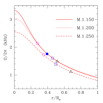
Clearly, corresponds to a star in uniform rotation, while corresponds to a star with increasing degree of differential rotation. As a reference, yields a star with an angular-velocity profile which varies of a factor between the center and the surface of the star (cf. left panel of figure 2).
In practice, we have computed a very large number of initial models using the SLy prescription for the EOS for which we have computed baryonic mass , the gravitational mass , the angular momentum , the rotational kinetic energy and the gravitational binding energy defined as
| (9) | |||||
| (10) | |||||
| (11) |
where is the square root of the determinant of three-dimensional metric and is the fluid Lorentz factor. We stress that the definitions (9)–(11) of quantities such as , , and are meaningful only in the case of stationary axisymmetric configurations and should therefore be treated with care once the rotational symmetry is lost.
| Model | |||||||||
|---|---|---|---|---|---|---|---|---|---|
| () | () | (Km) | |||||||
| M.1.140 | |||||||||
| M.1.150 | |||||||||
| M.1.160 | |||||||||
| M.1.180 | |||||||||
| M.1.200 | |||||||||
| M.1.210 | |||||||||
| M.1.220 | |||||||||
| M.1.230 | |||||||||
| M.1.241 | |||||||||
| M.1.244 | |||||||||
| M.1.247 | |||||||||
| M.1.250 | |||||||||
| M.2.125 | |||||||||
| M.2.150 | |||||||||
| M.2.175 | |||||||||
| M.2.200 |
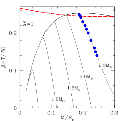
Out of this large set, we have then selected for the numerical evolution a number of models so as to build sequences of constant baryonic mass with , degree of differential rotation and values of the instability parameter ranging between and . Each model in this sequence is supramassive, namely it has a mass which is larger than the maximum mass allowed for a corresponding nonrotating model, i.e. , although it is not hypermassive, namely it does not have mass which is above the maximum mass for a uniformly rotating model, i.e. . There are two different reasons why such a large-mass model has been chosen. The first one is that we are interested in the development of a shear instability in the metastable star produced by the merger of a binary system of two neutron stars. As shown by a number of authors and most recently in [49], the product of this merger is either a supramassive or a hypermassive neutron star. Hence, our reference model has a mass which is sufficiently large so as to be a reasonable approximation to the product of a binary neutron star merger222We note that the use of a supramassive model has also the inconvenient consequence that it is not possible to construct a corresponding nonrotating model and this prevents us, for instance, from computing the frequency of the fundamental mode and compare it with the results of perturbative analyses.. The second reason is that a sufficiently massive model is necessary in order to reach values of the instability parameter which are above the expected threshold for dynamical bar-mode instabilities as computed in [7], i.e. . Indeed, the maximum possible value for within the computed sequence is around and thus just above the threshold (cf. long-dashed line in the left panel of figure 1). Note also that the threshold for the instability tends to increase for smaller rest-masses.
Overall, when comparing with equilibrium models generated with a polytropic EOS with and (see table 1 of [6]) the realistic EOS models reach higher compactness (models in [6] typically have ) but lower values of (i.e. for the models considered here, while for the polytropic models considered in [6]).
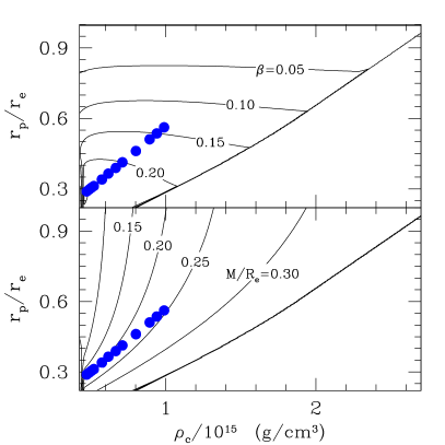
The whole space of parameters is shown in figure 1, whose left panel reports the position in the plane of the initial models computed with , and where the filled circles represent those we have evolved numerically. Indicated with solid thin lines are isocontours of constant baryon mass models while indicated with a thick dashed line is the threshold to the dynamical bar-mode instability as computed for a polytrope [7]. The right panel reports the same initial models considered in the left one but shown in planes with isocontours of constant (upper part) or constant (lower part). The main properties of the simulated models are also reported in table 1, where we also introduce our naming convention. Any initial model is indicated as M.%.#, with % being replaced by the value of the differential-rotation parameter and # by the instability parameter . As an example, M.1.200 is the star with and .
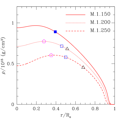
Finally, shown in figure 2 are the angular-velocity profiles (left panel) and the rest-mass density profiles (right panel) of some representative models, namely M.1.150, M.1.200 and M.1.250. Indicated with different symbols, which match the ones in the left panel of figure 5, are the normalized radial positions of the corotation radii, with the one for model M.1.150 being shown filled to help distinguish it from the others. Although we postpone to sections 4.1 and 4.2 the discussion of the implications of these corotation radii, two aspects of the initial data are worth emphasizing. The first one is that the amount of differential rotation for a given value of effectively decreases when increasing the instability parameter (cf. left panel of figure 2), thus resulting in a smaller corotation band for models with large . The second one is that all the initial models evolved are axisymmetric but have a “toroidal-topology”, namely have the maximum density that is not at the center of the star, and thus . This toroidal deformation increases with the rotation and thus with .
3 Methodology of the analysis
A number of different quantities are calculated during the evolution to monitor the dynamics of the instability. Among them is the quadrupole moment of the matter distribution
| (12) |
which we compute in terms of the conserved density rather than of the rest-mass density or of the component of the stress energy momentum tensor. Of course, the use of in place of or of is arbitrary and all the three expressions would have the same Newtonian limit, though with different amplitudes for the gravitational waveforms produced (see for example [53]). However, we here adopt the form (12) because is a quantity whose conservation is guaranteed by the form chosen for the hydrodynamics equations.
The quadrupole moment (12) can be conveniently used to quantify both the growth time of the instability and the oscillation frequency once the instability is fully developed . (Hereafter we will indicate respectively with and the growth time and frequencies of the unstable modes and we note that, as will be discussed later on, during the simulation a number of different modes appear, thus justifying the use of the upper index “”). In practice, we perform a nonlinear least-square fit of the component of the computed quadrupole and we generally use as fitting function a sum of (usually three) exponentially modulated cosines
| (13) |
where . Because we commonly have only about cycles in the time interval considered for the fits, extreme care needs to be applied when computing the growth time, especially when the oscillation frequencies and the growth times are close to each other. In these cases, in fact, variations of the initial phase of the modes can result in large variation of the growth times. In view of this, we will not report them.
Using three components of the quadrupole moment in the plane we can define the distortion parameters and , as well as the axisymmetric mode as
| (14) |
so that the modulus and the instantaneous orientation of the bar are given by
| (15) |
Finally, as a useful tool to describe the nonlinear properties of the development and saturation of the instability, the rest-mass density is decomposed into its Fourier modes as
| (16) |
The phase essentially provides the instantaneous orientation of the -th mode when the corresponding mode has a nonzero power. Note that despite their denomination, the Fourier modes (16) do not represent proper eigenmodes of oscillation of the star. While, in fact, the latter are well defined only within a perturbative regime, the former simply represent a tool to quantify, within the fully nonlinear regime, what are the main components of the rest-mass distribution. As a final comment we note that while all quantities (12)–(16) are expressed in terms of the coordinate time and are not invariant measurements, the lengthscale of variation of the lapse function at any given time is always larger than twice the stellar radius at that time, ensuring that events on the same timeslice are also close in proper time.
4 Results
In what follows we first describe the dynamics of the shear instability as deduced from the numerical simulations and then contrast our results with the phenomenological predictions on the necessary conditions for its development.
4.1 Dynamics of the instability
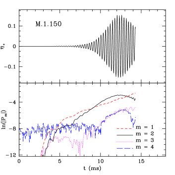
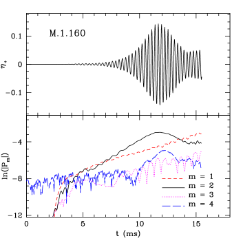
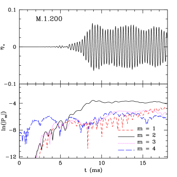
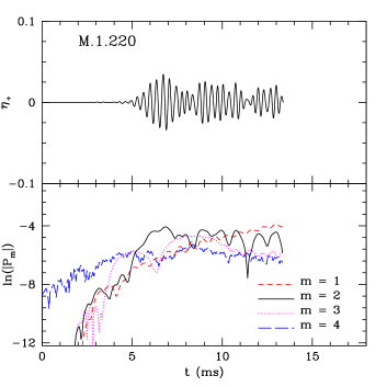
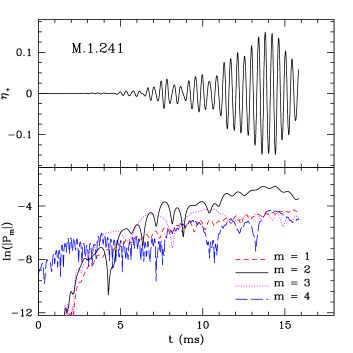
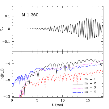
As mentioned when discussing the initial data, we have evolved numerically two sequences of constant baryonic mass, with . The first sequence has a higher degree of differential rotation (i.e. ) and instability parameter ranging from to . The second sequence, on the other hand, has a smaller degree of differential rotation (i.e. ) and instability parameter between and . For both sequences the highest value of considered is also very close to the highest attainable with our initial data code (see figure 1). To keep the computational costs to an affordable level we have evolved of all these models for and although this time window is in general insufficient to capture the suppression of the instability, is adequate to measure the frequencies of the unstable modes and provide a first estimate of the growth times.
After analyzing the results following the method outlined in the previous section and focusing on the properties of the distortion parameters , and , we find that all of the models show an instability. The maximum distortions obtained during the simulation time are (i.e. distortions of with respect to the axisymmetric progenitor), with the maximum values being reached for the models of the sequence. The models of the sequence, in fact, have in general much smaller distortions, with over the timescale over which they have been evolved. We believe this is simply the consequence of the fact that the models in this sequence have smaller growth rates (see also the discussion in the next section).
To show the general behaviour of the simulation we focus on the description of the result of the simulation for the sequence as this is representative also of the one with . In particular, in the upper part of each panel in figure 3 we show the time evolution of the distortion parameter computed with Eq. (14) for six representative models: M.1.150, M.1.160, M.1.200, M.1.220, M.1.241 and M.1.250. Similarly, in the lower parts of each panel we show the corresponding evolution of the Fourier-modes computed from Eq. (16) for .
Note that for models with lower values of the bar-mode deformation is very similar to the one already discussed in [6, 7], growing exponentially and with only one unstable mode appearing (cf. first row of figure 3). However, as the rotation is increased, the development of the instability is more complex and at least two unstable modes appear which develop in different parts of the star. These two modes have very similar but distinct frequencies and growth times, leading to a series of beatings in the evolutions of , whose irregular evolution makes the calculation of the growth times challenging (cf. second row). As the rotation is increased towards the maximal values of , up to three distinct modes appear and the evolution of the instability is correspondingly more complex (cf. third row). A similar behaviour is shown also by the evolution of the Fourier modes. The two models with lower , in fact, show a clear growth of the mode and of the , with the latter becoming first comparable and then larger when the instability is suppressed. In models M.1.250, M.1.241, on the other hand, the and modes have comparable amplitude for a long period and then the becomes the dominant one (this is more clear in model M.1.241). Finally, for larger values of , the mode never attains values comparable with either the or the , which instead control the evolution.
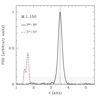
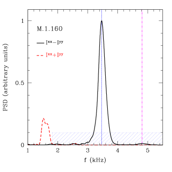
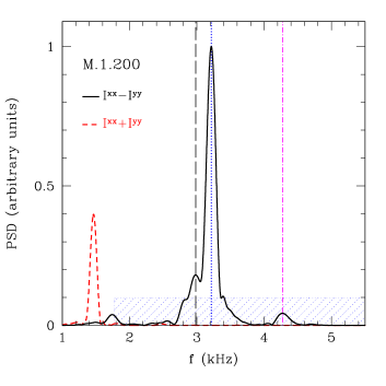
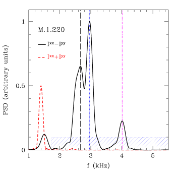
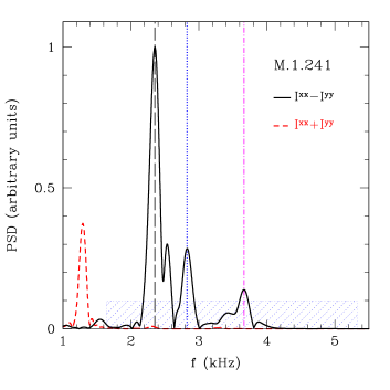
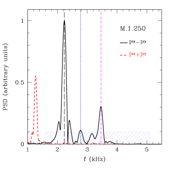
Figure 4 reports the power spectral density (PSD) of and for the same models (solid black lines) and allows to appreciate how the spectrum changes as the instability parameter is increased. More specifically, it is very apparent that at low the spectra have only one peak, whose maximum is marked by the vertical blue dotted lines and that is present at all the values of beta considered; this is the mode we refer to as (cf. table 2 and figure 5). As increases, the amplitude of this peak decreases and it becomes the weakest for very large rotation rates. Starting from model M.1.200 (although a hint of a peak is present already in M.1.160), a second peak appears at higher frequency and is marked with magenta vertical dot-dashed lines; this is the mode we refer to as and although it never becomes the largest one, its amplitude increases with . Finally, a third peak appears at low frequency in the spectra starting from model M.1.220 (even though a hint is present also for model M.1.210) and is marked with black vertical long-dashed lines. This mode, which we refer to as , becomes the dominant one at high . Note also that in each panel of figure 4 we report with a dashed blue box the corotation band that will be further discussed in the following section.
As a final remark we note that the peaks in the spectrum of (red dashed lines in figure 4) are related to axisymmetric modes and most likely to -modes oscillation excited by the development of the instability. Indeed, their frequencies match reasonably well the phenomenological fit for the -mode frequencies of nonrotating neutron stars with realistic EOSs computed in [54]. Because our sequences do not contain nonrotating configurations (the rest mass is larger than the maximum one), this association is just qualitative and a more detailed investigation of the frequency spectra of the equilibrium models is necessary to confirm this suggestion.
-
Model (kHz) (kHz) (kHz) (kHz) (kHz) (kHz) (kHz) (kHz) (kHz) M.1.140 M.1.150 M.1.160 M.1.180 M.1.200 M.1.210 M.1.220 M.1.230 M.1.241 M.1.244 M.1.247 M.1.250 M.2.125 M.2.150 M.2.175 M.2.200
4.2 Necessary conditions for the instability
To support the interpretation of these instabilities as shear instabilities we have considered whether the necessary conditions suggested by [2] and by [20] are met. We recall that Watts and collaborators pointed out that an unstable configuration should have the unstable mode with a frequency within the corotation band. In the case of the Newtonian expression (8), the corotation band is simpler to compute and for a mode with frequency and azimuthal number , this is simply given by
| (17) |
We have therefore checked whether any of the unstable (bar-modes) with computed frequency has pattern speed velocity, , within the corotation band. A careful and rather involved analysis has indeed confirmed the prediction of Watts and collaborators: namely, all the unstable modes are within the corotation band of the progenitor axisymmetric model. These results for the models with are listed in table 2, where we report the edges of the general-relativistic corotation band in terms of angular frequency at the surface and on the axis , as well as the frequencies of the unstable modes obtained from the position of the peaks in the PSD (i.e. ) or from the nonlinear fitting of Eq. (13) (i.e. ). Note that depending on the rate of rotation and the degree of differential rotation some frequencies may not be present in the corotation band.
The data in table 2 is also shown in the left panel of figure 5, where we plot the position of the non-axisymmetric frequencies within the corotation band as a function of ; indicated with a filled symbol, to distinguish it from the others, is the frequency for model M.1.150 (cf. figure 2 and 6). The right panel of the same figure shows the corresponding information and on the same scale but for the models with (the inset shows instead a magnified view). Clearly, for both sequences all the unstable modes are within the band and, as the stellar rotation rate increases, more unstable modes appear for the same value of .
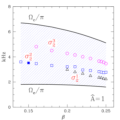
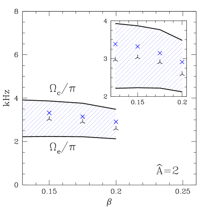
Watts, Andersson and Jones also give a qualitative description, summarized in their figure 2 of [2], of how the unstable and stable models should be distributed in the () plane. The considerations they make are particularly simple: for high degrees of differential rotation, that is at low values of , the corotation band is rather wide and there will be both an upper value and a lower value of between which the shear instability can develop (these critical values of correspond to the entrance and exit of the unstable mode in the corotation band). This situation corresponds therefore to the one commonly encountered in numerical simulations, such as those in [18, 19, 20, 21, 22, 23, 24], and for which the shear instability takes place only for very small values of the instability parameter and on timescales that are much longer than the dynamical one. When moving to larger degrees of differential rotation, that is when going to smaller values of , the corotation band becomes larger and larger and the shear instability can develop essentially for all values of , merging with the dynamical bar-mode instability for . This is exactly what has been found here. Conversely, when moving to smaller degrees of differential rotation, that is when going to higher values of , the corotation band becomes thinner and the shear instability can develop only for a smaller range of . As the differential rotation is further decreased and the star tends to rotate uniformly, the corotation band width vanishes, all the models are stable to the shear instability and subject only to the dynamical bar-mode instability for . This is indeed the case for the unstable models evolved in [6], which were purely (bar-mode) dynamically unstable and none of which had the unstable mode within the corresponding corotation band, but above it.
In essence, therefore, there should be an intermediate range of for which the instability is absent at low , appears at intermediate values and then disappears again at high , thus defining an interval of values of for which the models are unstable. To validate also this prediction we simulated a sequence of models with smaller differential rotation and . This seconds sequence has the same baryonic mass as that with , but with in a smaller range, namely between and (Note that is also very close to the largest value for which we could build an equilibrium model.) Unfortunately, also all of these models show an shear instability, with the unstable frequencies falling within the corotation band, as it was for the stars. Of course, lack of evidence is not evidence of absence and the fact that we have not found stable models within our range of values of most likely means that these stable models have to be searched either for values of (for this value of ), or by moving towards higher values of , where the corotation band is less large.
An obvious consequence of the phenomenological scenario described by [2] and confirmed by the calculations reported here is that the idea of a low- instability is indeed misleading and it is instead more meaningful to think of a more generic shear instability that, depending on the degree of rotation and of differential rotation, may manifest itself on timescales that are comparable with the dynamical ones (as in the cases reported here) or on much longer ones (as in the cases reported in [17]).
Another phenomenological prediction made by Watts, Andersson and Jones in [2], is that the growth times should be shorter in the center of the band and increase towards the edges (the growth times should in fact diverge at the edges). As shown in figure 5, all of the simulated models do have unstable modes well inside the corotation band and this probably explains why we observe them develop on a timescale which is comparable with the dynamical one and not on much longer timescales as in the original finding of [17]. We also find indications that the models, which generically have longer growth times, have unstable modes which occupy regions of the corotation band that are overall more central (cf. right panel of figure 5) and thus in contrast with what expected from [2]. However, the difficulties mentioned above in computing an accurate estimate of the growth times and the intrinsic difficulties in determining what is the central part of the corotation band, prevent us from providing a more quantitative validation of this prediction.
We now switch to consider our results in the light of the other necessary condition for the onset of the shear instability discussed in [20]. As mentioned in the Introduction, it has in fact been shown that the presence of a minimum in the profile of the vortensity is a necessary condition for a mode in corotation to be unstable [20]. The intuitive description is that the vortensity well can act as a resonant cavity inside the star, amplifying the modes that happen to lay near its minimum [32]. Indeed, the growth rate of the unstable mode is expected to depend on the location of its corotation radius with respect to the vortensity profile, being proportional to the depth of its corotation radius inside the vortensity well [20]. Note that the mere existence of a local minimum in the vortensity cannot be used as a sufficient condition for the occurrence of a shear instability. All of the unstable models considered in [6], in fact, do show a local minimum in the vortensity but do not have the unstable modes in the corotation band.
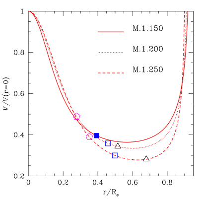
To validate whether this Newtonian condition holds also for the general-relativistic instabilities simulated here, we have computed for all the models the Newtonian vortensity, which is defined as the ratio, along the radial cylindrical coordinate, between the radial vorticity and the density
| (18) |
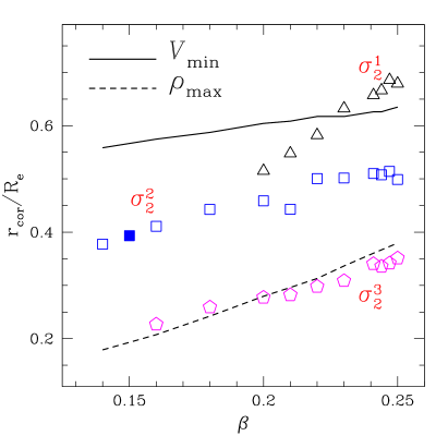
where is the radial cylindrical coordinate (a fully general-relativistic definition of the vortensity is also possible but more complicated to compute and not significantly different from the Newtonian one). When doing this we found that all the unstable models have vortensities with a local minimum in the star and this is shown in the left panel of figure 6, which reports the radial profiles of the vortensity for three representative models with small, medium and high values of . The different symbols match the ones in the left panel of figure 2 and 5, with the one for model M.1.150 reported as filled, and show the actual positions of the corotation radii. The right panel of the same figure, on the other hand, shows the normalized corotation radii for the different frequencies presented in the left panel of figure 5 as a function of .
Note that none of these coincides systematically with the minimum of , nor with the maximum of the rest-mass density. All of the corotation radii, however, do move towards larger radial positions as the rotation rate is increased, exactly as does the minimum of the vortensity and the rest-mass maximum. Although we cannot confirm that modes whose corotation radius is closer to the minimum of the vortensity have systematically shorter growth times (our data is not sufficiently accurate for this), we can compare the models with the higher degree of differential rotation with those having a smaller degree of differential rotation . In the first case the vortensity well is considerably deeper, with , while for the latter the vortensity has shallower wells with . Since the models with have smaller growth rates, our results indicate therefore that also the existence of a local minimum in the vortensity can be taken as a necessary condition for the development of the shear instability and that the depth of the vortensity well can be used to estimate the growth of the instability.
5 Conclusions
For many years the properties of rapidly rotating and self-gravitating fluids have been characterized by a complete analytic perturbative theory which provided, for instance, sufficient conditions for the development of instabilities (see, for instance, [3, 55] for a collection of results). As numerical simulations have become increasingly accurate and stable on longer timescales, these predictions, both in Newtonian theory and in full general relativity, have been verified, corrected and in some cases extended. Our ability of modelling such configurations has now reached a maturity such that a number of new properties and instabilities have been “discovered” numerically, but which do not have behind a fully perturbative description. The main reason for this is that most of this phenomenology is the result of physical scenarios which are much more complex than the ones investigated perturbatively in the past, e.g. non-isolated systems with high differential rotation and exchanging mass and angular momentum, which are much more difficult to treat analytically.
A most notable example of these complex and yet ubiquitous instabilities is the so-called “low- instability”, which was initially found in [17] and then reproduced in a number of other different scenarios [18, 19, 20, 21, 22, 23, 24, 25]. As the phenomenological description of this instability provided by the simulations has become richer and richer, a full understanding of the mechanisms that lead to its development has lagged behind and it is presently unclear. We are therefore in a situation in which numerical simulations can probe regimes and conditions which are not yet accessible to perturbative calculations, and can guide the latter by confirming or refuting those scenarios that although possible do not find a realization in practice.
This work has followed this spirit and has used fully general-relativistic calculations of rapidly and differentially rotating neutron stars modeled with a realistic EOS to shed some light on the development of the low- instability. In particular we have concentrated our attention on validating an indirect prediction, made by Watts, Andersson and Jones [2], who recognized the low- instability as the manifestation of a more generic class of instabilities associated to the existence of a corotation band [30, 31], the shear instabilities, and that should develop for any value of the instability parameter when sufficient amounts of differential rotation are present. This is exactly what we have found in our simulations. More specifically, we have performed simulations of sequences of neutron-star models described by a realistic SLy EOS [1] and having constant rest-mass and degrees of differential rotation, but with different amounts of rotation. In all cases considered we have found the development of a bar-mode instability growing on a dynamical timescale, even when the initial axisymmetric models were well below the critical limit for the dynamical bar-mode instability. These results, which match well the phenomenological scenario portrayed in [2], suggest therefore that the idea of a low- instability is indeed misleading and should be replaced by the more general one of shear instability. Depending then on the degree of rotation and of differential rotation, the instability will develop on timescales that are comparable to the dynamical one (as reported here) or on much longer ones (as reported in the first low- instability studies).
Special attention has also been paid to the properties of the unstable modes and to their position within the corotation band or the vortensity profiles. In particular, we have shown that all the unstable modes are within the corotation band of the progenitor axisymmetric model (which is the necessary condition for the development of the instability proposed by [2]) and that all of the unstable models have vortensity profiles with a local minimum (which is the necessary condition suggested by [20]). Finally, by comparing the growth times among models with different degree of differential rotation we have shown that there is a correlation, although not a strong one, between the depth of the vortensity well and growth rate of the instability, with the latter being larger for models with deeper wells.
In summary, the results presented here shed some light on several aspects of shear instabilities, but they also reveal that more work is required, for instance, to distinguish between the predictions based on the corotation band and the ones based on the vortensity well, or to establish whether in effect they just represent two different ways of expressing the same physical conditions. Clarifying these aspects will requires additional analytical and numerical modelling, and this will be part of our future research.
References
References
References
- [1] Douchin F and Haensel P 2001 Astronomy and Astrophysics 380 151–167
- [2] Watts A L, Andersson N and Jones D I 2005 Astrophys. J. 618 L37
- [3] Chandrasekhar S 1969 Ellipsoidal Figures of Equilibrium (New Haven, USA: Yale University Press)
- [4] Saijo M, Shibata M, Baumgarte T W and Shapiro S L 2001 Astrophys. J. 548 919–931
- [5] Shibata M, Baumgarte T W and Shapiro S L 2000 Astrophys. J. 542 453–463
- [6] Baiotti L, De Pietri R, Manca G M and Rezzolla L 2007 Phys. Rev. D. 75 044023
- [7] Manca G M, Baiotti L, Pietri R D and Rezzolla L 2007 Class. Quantum Grav. 24 S171–S186
- [8] Brown J D 2000 Phys. Rev. D 62 084024
- [9] Houser J L and Centrella J M 1996 Phys. Rev. D 54 7278–7297
- [10] Liu Y T 2002 Physical Review D 65 124003
- [11] New K C B, Centrella J M and Tohline J E 2000 Physical Review D 62 064019
- [12] Pickett B K, Durisen R H and Davis G A 1996 Astrophys. J. 458 714
- [13] Camarda K D, Anninos P, Fragile P C and Font J A 2009 Astrophys. J. 707 1610–1622
- [14] Saijo M and Kojima Y 2008 Phys. Rev. D 77 063002
- [15] Chandrasekhar S 1970 Physical Review Letters 24 611–615
- [16] Friedman J L and Schutz B F 1978 Astrophys. J. 222 281–296
- [17] Shibata M, Karino S and Eriguchi Y 2002 Mon. Not. Roy. Astron. Soc. 334 L27
- [18] Shibata M, Karino S and Eriguchi Y 2003 Mon. Not. Roy. Astron. Soc. 343 619
- [19] Ott C D, Ou S, Tohline J E and Burrows A 2005 Astrophys. J. 625 L119–L122
- [20] Ou S and Tohline J E 2006 Astrophys. J. 651 1068
- [21] Cerdá-Durán P, Quilis V and Font J A 2007 Computer Physics Communications 177 288–297
- [22] Ott C D, Dimmelmeier H, Marek A, Janka H, Hawke I, Zink B and Schnetter E 2007 Physical Review Letters 98 261101
- [23] Ott C D, Dimmelmeier H, Marek A, Janka H, Zink B, Hawke I and Schnetter E 2007 Classical and Quantum Gravity 24 139
- [24] Scheidegger S, Fischer T, Whitehouse S C and Liebendörfer M 2008 Astronomy and Astrophysics 490 231–241
- [25] Abdikamalov E B et al. 2009 arXiv:0910.2703
- [26] Watts A L, Andersson N, Beyer H and Schutz B F 2003 Mon. Not. Roy. Astron. Soc. 342 1156
- [27] Rezzolla L and Yoshida S 2001 Classical and Quantum Gravity 18 L87–L94
- [28] Abramowicz M A, Rezzolla L and Yoshida S 2002 Classical and Quantum Gravity 19 191–194
- [29] Saijo M and Yoshida S 2006 Mon. Not. Roy. Astron. Soc. 368 1429–1442
- [30] Balbinski E 1985 Mon. Not. Roy. Astr. Soc. 216 897–908
- [31] Luyten P J 1990 Mon. Not. Roy. Astr. Soc. 242 447–456
- [32] Papaloizou J C B and Lin D N C 1989 Astrophys. J. 344 645–668
- [33] Pollney D, Reisswig C, Rezzolla L, Szilágyi B, Ansorg M, Deris B, Diener P, Dorband E N, Koppitz M, Nagar A and Schnetter E 2007 Phys. Rev. D76 124002
- [34] Mösta P, Palenzuela C, Rezzolla L, Lehner L, Yoshida S and Pollney D Phys. Rev. D, 81 064017 (2010)
- [35] Banyuls F, Font J A, Ibáñez J M, Martí J M and Miralles J A 1997 Astrophys. J. 476 221
- [36] Baiotti L, Hawke I, Montero P and Rezzolla L 2003 Computational Astrophysics in Italy: Methods and Tools vol 1 ed Capuzzo-Dolcetta R (Trieste: MSAIS) p 210
- [37] Baiotti L, Hawke I, Montero P J, Löffler F, Rezzolla L, Stergioulas N, Font J A and Seidel E 2005 Phys. Rev. D 71 024035
- [38] Baiotti L, Hawke I and Rezzolla L 2007 Class. Quantum Grav. 24 S187–S206
- [39] Giacomazzo B, Rezzolla L and Baiotti L 2009 Mon. Not. R. Astron. Soc. 399 L164–L168
- [40] Harten A, Engquist B, Osher S and Chakrabarty S R 1987 J. Comput. Phys. 71 231
- [41] Colella P and Woodward P R 1984 J. Comput. Phys. 54 174
- [42] Harten A, Lax P D and van Leer B 1983 SIAM Rev. 25 35
- [43] Roe P L 1981 J. Comput. Phys. 43 357
- [44] Aloy M A, Ibáñez J M, Martí J M and Müller E 1999 Astrophys. J. Supp. 122 151
- [45] Schnetter E, Hawley S H and Hawke I 2004 Class. Quantum Grav. 21 1465–1488
- [46] Haensel P and Pichon B 1994 Astronomy and Astrophysics 283 313–318
- [47] Baym G, Pethick C and Sutherland P 1971 Astrophys. J. 170 299
- [48] Haensel P and Potekhin A Y 2004 Astron. Astrophys. 428 191–197
- [49] Baiotti L, Giacomazzo B and Rezzolla L 2008 Phys. Rev. D 78 084033
- [50] Swesty F D J. Comput. Phys. 127 1 118-27 (1996)
- [51] Shibata M, Taniguchi K and Uryū K 2005 Phys. Rev. D 71 084021
- [52] Stergioulas N and Friedman J L 1995 Astrophys. J. 444 306
- [53] Baiotti L, Bernuzzi S, Corvino G, De Pietri R and Nagar A 2009 Phys. Rev. D79 024002
- [54] Benhar O, Ferrari V and Gualtieri L 2004 Phys. Rev. D70 124015
- [55] Lai D, Rasio F A and Shapiro S L 1993 Astrophys. J., Suppl. Ser. 88 205–252