A Measurement of Cubic-Order Primordial Non-Gaussianity ( and )
With WMAP 5-Year Data
Abstract
We measure two higher-order power spectra involving weighted cubic and squared temperature anisotropy maps from WMAP 5-year data to study the trispectrum generated by primordial non-Gaussianity. Using these measurements combined with Gaussian and noise simulations, we constrain the cubic order non-Gaussianity parameters , and . With V+W-band data out to , we find and improving the previous COBE-based limit on nearly four orders of magnitude with WMAP. We find that the ratio of trispectrum to bispectrum amplitude as captured by the ratio of ranges from -3 to 21 at the 95% confidence level.
pacs:
98.70.Vc, 98.80.-k, 98.80.Bp, 98.80.EsIntroduction.—Cosmic Inflation has deservedly become a cornerstone of modern cosmology Guth:1980zm ; Linde:1981mu ; Albrecht:1982wi . Inflation solves the flatness, horizon and the monopole problems of the standard Big-Bang cosmology. Furthermore, inflation is the prevailing paradigm related to the origin of density perturbations that gave rise to the large-scale structure we see in the universe. It posits that a nearly exponential expansion stretched space in the first moments of the early universe and promoted microscopic quantum fluctuations to perturbations on cosmological scales today GuthPi ; Bardeen .
In the simple scenario, inflation is driven by a single scalar field whose potential energy dominates it’s kinetic energy. This “slow-roll” situation leads to an exponential expansion of the cosmic spacetime via the Einstein equations coupled to a scalar field. In order to maintain a slow roll, the scalar field must have minimal self interactions. Such a non-interacting field has the statistical feature that its fluctuations are Gaussian. A Gaussian field contains no correlations between points arising from interactions.
In addition to the standard inflationary scenario, several possible mechanisms of inflation have emerged. These models usually involve multiple fields and or other exotic objects such as branes (motivated by string theory) that have non-trivial interactions. These interactions produce a departure from Gaussianity in a model-dependent manner Byrnes:2010em ; Engel:2008fu ; Chen:2009bc ; Boubekeur:2005fj . Constraining non-Gaussianity therefore is important to distinguish between the plethora of inflationary models Komatsu:2009kd .
The first order non-Gaussian parameter, , has been measured with increasing success in the bispectrum, or three-point correlation function of temperature anisotrpies of the cosmic microwave background (CMB). Such studies have found to be consistent with zero Yadav:2007yy ; Smith:2009jr ; Komatsu:2010fb ; Smidt:2009ir .
In addition to , with the trispectrum or four point correlation function of CMB anisotrpies, we can measure second order non-Gaussian parameters and . Constraints on have never been directly preformed with data. The very weak constraint often quoted in the literature with is an estimate based on a null detection of the COBE data Boubekeur:2005fj ; Kunz:2001ym ; Komatsu:2002db . Furthermore, the ratio between and , involving the amplitudes of trispectrum and bispectrum, is often is often a constraint on inflationary models Byrnes:2010em ; Chen:2009bc . In fact, for many inflationary models this ratio is related to the tensor-to-scalar ratio, which is now probed by CMB polarization data, providing additional consistency relations to understand the underlying physics of inflation Byrnes:2010em . Constraints on have only recently been preformed, but not with the trispectrum of the CMB Vielva:2009jz .
In this analysis we use the trispectrum, or the four-point correlation function of temperature anisoptropies, to measure primordial non-Gaussianity at second order using WMAP 5-year data Hu:2001fa .
Theory.— To parameterize the non-Gaussianity of a nearly Gaussian field, such as the primordial curvature perturbations , we can expand it perturbatively Kogo:2006kh to second order as:
| (1) |
where is the purely Gaussian part with and parametrizing the first and second order deviations from Gaussianity. Fortunately, information about the curvature perturbations are contained within the CMB through the spherical harmonic coefficients of the temperature anisotropies:
| (2) | |||||
| (3) |
where are the primordial curvature perturbations, is the radiation transfer function, is the field of temperature fluctuations in the CMB and ’s are the spherical harmonics.
If the curvature perturbations are purely Gaussian, all the statistical information we can say about them is contained in the two point correlation function . The information contained in the two point function is usually extracted in spherical harmonic space, leading to the power spectrum , defined by:
| (4) |
However, if the curvature perturbations are slightly non-Gaussian, this two point function is no longer sufficient to articulate all the information contained in the field. With non-Gaussianity, extra information can be extracted from the three, four and higher n-point correlation functions.
In this paper we look to the trispectrum, or four point correlation function, to probe non-Gaussianity. To extract information from the four point function , we again work in spherical harmonic space and compute:
| (5) | |||||
where we see that the four point function breaks up into a piece representing a Gaussian contribution and a second piece representing the non-Gaussian contribution. The non-Gaussian piece is commonly referred to as the connected piece and is generated by interactions between points.
As with the two point function, from the four point function we can create various power spectra. Two independent spectra that can be produced are and (See Fig. 1) that are related to various compressions of s as follows:
| (6) |
Here should be read as is related to as the full expression is very complex. (We refer the reader to Refs. Munshi:2009wy for full details of the derivation of eq. 6 including the pre-factors.). The superscript in the refers to how many temperature maps must be combined to form the . For example, only one is used in eq. 3-4.In the same manner is the angular power spectrum of temperature and and are the angular power spectrum of squared-temperature correlated against squared temperature and cubic temperature correlated against temperature, respectively. To optimize for primordial non-Gaussianity detection, however, the temperature maps used for and are weighted appropriately in the same manner we optimized statistic for the bispectrum measurement Smidt:2009ir .
The estimators and contain contributions from the Gaussian and connected piece of equation 5. The connected piece further breaks up into two independent pieces parameterized by two parameters and :
| (7) | |||||
| (8) |
Here, and are the theoretical expectations for the connected part of and with the assumption that and respectively.
It is clear from equation 1 that is a non-Gaussian parameter of second order. Additionally, in a derivation of the trispectrum one finds that is related to in a model dependent way, and is therefore also a second order parameter.
Since the exact relation between from the trispectrum and from the bispectrum is model dependent, this relationship gives another test to distinguish between models for primordial perturbations Byrnes:2010em ; Engel:2008fu ; Chen:2009bc ; Boubekeur:2005fj . It is common to compare with and therefore we constrain the relation where is the amplitude of the trispectrum to the squared bispectrum. For many models can be used to further constrain the tensor-to-scalar ratio Byrnes:2010em .
Analysis and Results.—Our recipe for analysis is
-
1.
We calculate , , and in Eq. 7- 8 for and . (See Munshi:2009wy for more details on how to do this and other steps.)
-
2.
We extract and directly from WMAP 5-year data.
-
3.
We preform the extraction of and from 250 Gaussian maps, allowing us to determine error bars and the Gaussian piece of each estimator.
-
4.
We subtract off the Gaussian contribution to these estimators to ensure we are fitting to the non-Gaussian contribution.
-
5.
We fit the two unknowns and from data using the two equations simultaneously. The amplitudes the theoretical curves must be scaled by gives the values for and
-
6.
We constrain by comparing from the trispectrum with coming from the bispectrum.
This recipe is described in grater detail below:
First we calculate , , and theoretically using the full equations described in Munshi:2009wy . To obtain we use CAMB Lewis:1999bs 222 with the WMAP 5-year best fit parameters and use the beam transfer functions from the WMAP team. We then obtain the connected piece using a modified version of the CMBFAST code Seljak:1996is 333. Plots of many of the quantities used for these calculations can be found in Ref. Smidt:2009ir .
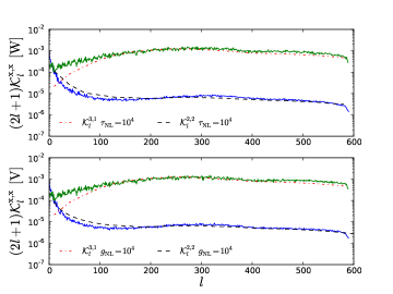
We combine , with various assumed values of and to establish and . These are plotted in Figure 1. These curves will be compared with estimators derived from data to determine the magnitude of each statistic. Since we have two estimators, we can solve for the two unknowns and by fitting both estimators simultaneously.
To calculate444see Smidt el al. 2009 for a similar calculation using the bispectrum for more details. Smidt:2009ir the estimators from data, used in the lefthand side of equations (7) and (8), we use both the raw and foreground-cleaned WMAP 5-Year Stokes I maps for V- and W-bands masked with the KQ75 mask 555. We use the Healpix library to analyze the maps. For this analysis we only considered data out to . We correct for the KQ75 mask using a matrix , based on the power spectrum of the mask, as described in Munshi:2009wy .
Figure 1 shows the results for and for the V and W frequency bands extracted from the raw WMAP 5-Year maps.

In order to do proper statistics for our data fitting we create 250 simulated Gaussian maps of each frequency band with . To obtain Gaussian maps we run the synfast routine of Healpix with an in-file representing the WMAP 5-year best-fit CMB anisotropy power spectrum and generate maps with information out to . We then use anafast, without employing an iteration scheme, masking with the mask, to produce ’s for the Gaussian maps out to . Obtaining estimators from these Gaussian maps allows us to uncover the Gaussian contribution to each estimator in addition to providing us information needed to calculate the error bars on our results.
This whole process is computationally intensive. To calculate all theoretical estimators took nearly 8,000 CPU hours. Furthermore, all the estimators from Gaussian and data maps combined took an additional 1600 CPU hours.


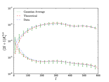
As previously discussed, the full trispectrum can be decomposed into both a Gaussian and non-Gaussian or connected piece. To make a measurement of non-Gaussianity we to subtract off the Gaussian piece from the full trispectrum. Figure 2 shows the the relationship between the full trispectrum and the Gaussian piece. In this plot the Gaussian piece was calculated in two different ways as a sanity check. First, the Gaussian maps were averaged over. Second, the Gaussian piece of each estimator is calculated theoretically as described inMunshi:2009wy .
| Band | W | V | V+W |
|---|---|---|---|
| Raw | |||
| FC | |||
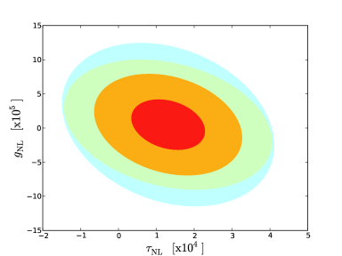
After obtaining the theory, data and simulated curves we use the best fitting procedure described in Smidt:2009ir where we minimize to fit and simultaneously. Our results are listed in Table 1. We see that and are consistent with zero with 95% confidence level ranges and for V+W-band in foreground-cleaned maps. The 95% confidence intervals of versus are plotted in Figure 3 for each band. Furthermore, we find that the constraint .
Conclusion.—This paper gives the first direct constraints on and improves the previous indirect estimate by four orders of magnitude. Our limit on is close to a level where interesting constraints can started to be placed on models available in the literature for primordial perturbations, such as due to cosmic stringsEngel:2008fu .
Furthermore, this paper is the first to constrain . This quantity is a model dependent relation between and , that for some models can be used to further constrain the tensor-to-scaler-ratio. We uncover that that the data is consistent with values between -3 and 21 at 95% confidence. Moreover, models with largely negitive, such as some arising from DBI inflation are disfavored Engel:2008fu .
Acknowledgements.
We are grateful to Eiichiro Komatsu, and Kendrick Smith for assistance during various stages of this work. This work was supported by NSF CAREER AST-0645427 and NASA NNX10AD42G at UCI and STFC rolling grant ST/G002231/1 (DM).References
- (1) A. H. Guth, Phys. Rev. D 23, 347 (1981).
- (2) A. D. Linde, Phys. Lett. B 108, 389 (1982).
- (3) A. J. Albrecht and P. J. Steinhardt, Phys. Rev. Lett. 48, 1220 (1982).
- (4) A. H. Guth and S. Y. Pi, Phys. Rev. Lett. 49, 1110 (1982).
- (5) J. M. Bardeen, P. J. Steinhardt and M. S. Turner, Phys. Rev. D 28, 679 (1983).
- (6) L. Boubekeur and D. H. Lyth, Phys. Rev. D 73, 021301 (2006)
- (7) K. T. Engel, K. S. M. Lee and M. B. Wise, Phys. Rev. D 79, 103530 (2009)
- (8) X. Chen, B. Hu, M. x. Huang, G. Shiu and Y. Wang, JCAP 0908, 008 (2009)
- (9) C. T. Byrnes and K. Y. Choi, arXiv:1002.3110 [astro-ph.CO].
- (10) E. Komatsu et al., arXiv:0902.4759 [astro-ph.CO].
- (11) A. P. S. Yadav and B. D. Wandelt, Phys. Rev. Lett. 100, 181301 (2008)
- (12) K. M. Smith, L. Senatore and M. Zaldarriaga, JCAP 0909, 006 (2009)
- (13) E. Komatsu et al., arXiv:1001.4538 [astro-ph.CO].
- (14) J. Smidt, A. Amblard, P. Serra and A. Cooray, Phys. Rev. D 80, 123005 (2009)
- (15) M. Kunz et al. ApJL 563, L99 (2001)
- (16) E. Komatsu, arXiv:astro-ph/0206039.
- (17) P. Vielva and J. L. Sanz, arXiv:0910.3196 [astro-ph.CO].
- (18) W. Hu, Phys. Rev. D 64, 083005 (2001)
- (19) N. Kogo and E. Komatsu, Phys. Rev. D 73, 083007 (2006)
- (20) D. Munshi, A. Heavens, A. Cooray, J. Smidt, P. Coles and P. Serra, arXiv:0910.3693 [astro-ph.CO].
- (21) A. Lewis, A. Challinor and A. Lasenby, Astrophys. J. 538, 473 (2000)
- (22) U. Seljak and M. Zaldarriaga, Astrophys. J. 469, 437 (1996)