EIGENVALUE DISTRIBUTIONS FOR A CLASS OF COVARIANCE MATRICES
WITH APPLICATIONS TO BIENENSTOCK-COOPER-MUNRO NEURONS UNDER NOISY CONDITIONS

Abstract

We analyze the effects of noise correlations in the input to, or among, BCM neurons using the Wigner semicircular law to construct random, positive-definite symmetric correlation matrices and compute their eigenvalue distributions. In the finite dimensional case, we compare our analytic results with numerical simulations and show the effects of correlations on the lifetimes of synaptic strengths in various visual environments. These correlations can be due either to correlations in the noise from the input LGN neurons, or correlations in the variability of lateral connections in a network of neurons. In particular, we find that for fixed dimensionality, a large noise variance can give rise to long lifetimes of synaptic strengths. This may be of physiological significance.

I Introduction

Receptive field changes in visual cortex, observed in the early period of an animal’s postnatal development, are thought to depend on synaptic plasicityBear and Rittenhouse (1999); Sengpiel and Kind (2002); the detailed dynamics of such receptive field modifiability has been used to infer the precise form of this plasticityBlais et al. (1998); Cooper et al. (2004). In a classic paradigm, called monocular deprivation, vision through one eye is deprived in early development. In this case cells in visual cortex tend to disconnect from deprived eyeWiesel and Hubel (1962). Experiments have shown that if monocular deprivation is produced by monocular lid closure then a rapid loss of response to the deprived eye occurs, while if the retina is inactivated by a Tetrodotoxin (TTX) injection, significantly less loss is observedRittenhouse et al. (1999); Frenkel and Bear (2004). These results are consistent with the form of synaptic plasticity proposed by Bienenstock, Cooper and Munro (BCM)Bienenstock et al. (1982). The BCM theory was originally proposed to describe plasticity processes in visual cortex as observed by Hubel and Wiesel Wiesel and Hubel (1962). One of the main postulates of this theory is the existence of a critical threshold (the sliding threshold) that depends on past neuronal history in a non-linear way. This nonlinearity is necessary to ensure stability of the synaptic weights. The main predictions of the BCM theory have been confirmed in hippocampal slices and visual cortex and recently in in vivo inhibitory avoidance learning experimentsWhitlockand et al. (2006). The extension of these results to other brain areas, and ultimately to the whole brain, is not confirmed but is under active study. One motivation for this research is that a proposed biophysical mechanism for the BCM rule is based on calcium influx through NMDA receptors and phosphorylation state of AMPA receptors and that both receptors are widely distributed within the brainCastellani et al. (2001). This biophysical mechanism is at least partly shared, by the plasticity rule STDP (Spike-timing-dependent plasticity)Abbott and B.Nelson (2000) that describes the synaptic functional change on the basis of action potentials timing in connected neurons. The main difference between STDP and BCM is that BCM is an average time rule and thus does not include microscopic temporal structures (i.e. it works with rates not spikes)Gerstner et al. (1996); Gerstner and Kistler (2002). A further analysis that considers the relation between BCM and STDP rules will be considered in a future work.

The standard theoretical analysis of monocular deprivation experimental results, according to BCM (see for example Cooper et al. (2004)) relies on the, seemingly reasonable, assumption that in the inactivated situation, activity in the lateral geniculate nucleus (LGN), which is the cortical input, is reduced compared to the lid closure case; as a consequence there is a less rapid loss of response to the deprived eye. This assumption has been questioned by new experimental results.Arnold et al. (2009)

In this recent study the activity of neurons in LGN has been measured during normal vision, when the eye-lid of the experimental animals was sutured and when TTX was injected into the lid sutured eye. The recordings were made on awake animals while they watched movie clips and sinusoidal gratings. A surprising result of these experiments is that inactivation does not reduce mean activity in LGN compared to lid suture; however inactivation produced an increase in correlations between different cells within the LGN. Previous experimental results in ferret LGNWeliky and Katz (1999); Ohshiro and Weliky (2006), and further results in mouse LGNArnold et al. (2009) indicate that the activity of nearby cells in LGN are correlated, that this activity falls off as a function of the distance between the receptive fields of the cells, and that these correlations exist even in the absence of retinal activity.

A recent paperBlais et al. has examined the impact of input correlations during deprivation experiments and has shown that correlations in LGN noise can significantly slow down the loss of response to the deprived eye for BCM neuronsBienenstock et al. (1982), in agreement with experiments. This paper also examines the effect of such correlations on a class of PCA type learning rules. Thus correlated LGN noise theoretically leads to persistence of synaptic strength for a period that depends on the level of noise correlation. As a consequence, noise at neuronal level could play a fundamental role in synaptic plasticity. The effect of white noise on BCM has been previously studiedBazzani et al. (2003). In this paper we show that noise correlations in the input or among BCM neurons can be studied by using the eigenvalue distributions of random positive-definite symmetric matrices. In a simple but generic case, we explicitly compute the distribution by using the Wigner semicircular lawWigner (1958, 1967), pointing out the role of correlations and the existence of a thermodynamic limit. In the finite dimensional case, the analytic results are compared with numerical simulations with applications to real conditions. We also discuss a transition in the eigenvalue distribution when the noise level is increased. This phenomenon implies the existence of states with very long lifetimes; these could have physiological significance in the development of neuronal systems.

II BCM neuron in monocular deprivation

We briefly review the behavior of a Bienenstock, Cooper and Munro (BCM) neuronBienenstock et al. (1982) in monocular deprivation. Let $\mathbf{w}$ be the synaptic weights and $\mathbf{x}$ the input signals received by the synapses, the BCM synaptic modification rule has the form

$$\mathbf{\dot{w}}=\mathbf{x}\phi(y,\theta_{m})$$ (1)

where the modification function $\phi(y,\theta_{m})$ depends on the neuron activity level $y\propto\mathbf{x}\cdot\mathbf{w}$ (it is assumed a linear proportionality between the input $\mathbf{x}$ and the output $y$) and on a moving threshold $\theta_{m}$, which is a super-linear function of the cell activity history (in a stationary situation $\theta_{m}$ can be related to the time averaged value $<y^{k}>$ where $k>1$ of a non-linear moment of the neuron activity distribution)Cooper et al. (2004). The modification function $\phi$ is a non-linear function of the postsynaptic activity $y$ which has two zero crossings, one at $y$=0 and the other at $y=\theta_{m}$ (see fig. 1). When the neuron activity is above the threshold $\theta_{m}$ we have LTP, whereas LTD appears when the activity is below the threshold. The nonlinear dependence of the threshold on neuron activity solves the stability problem of Hebb’s learning rule, preventing a dynamical divergence of synaptic weights ($y=\theta_{m}$ is an attractive fixed point for a stationary input)Cooper et al. (2004). In the simplest form the function $\phi$ is a quadratic function $\phi(y)=y^{2}-y\theta_{m}$ and the dynamic threshold $\theta_{m}$ is the time-averaged $<y^{2}>$ of the second moment of the neuron activity, which can be replaced by the expectation value over the input probability space $E(y^{2})$ under the slow-learning assumption.

Figure 1: The BCM function $\phi(y)$; when $y$ is close to zero, we can linearize the system (1) by approximating $\phi\simeq-\epsilon y$.

During MD regime, the input signal $\mathbf{x}$ to the closed eye can be represented by a stochastic process with zero mean value and small variance ($<\mathbf{x}^{2}>\ll 1$). One can numerically study the effect of noise correlation by integrating the system (1). Let us introduce the input noise

$$\mathbf{x}(t)=A\xi(t)$$ (2)

where $\xi(t)$ is a stochastic process in $\mathbb{R^{N}}$ defined by i.i.d. random variables with zero mean value and normalized variance. We consider a symmetric matrix $A$ of the form

$$A={1\over\sqrt{1+q^{2}}}\begin{pmatrix}1&{q\over\sqrt{N}}a_{12}&...&{q\over\sqrt{N}}a_{1N}\\ {q\over\sqrt{N}}a_{12}&1&...&{q\over\sqrt{N}}a_{2N}\\ ..&..&...&..\\ {q\over\sqrt{N}}a_{1N}&{q\over\sqrt{N}}a_{2N}&...&1\end{pmatrix}\qquad N\gg 1$$ (3)

where the coefficients $a_{ij}$ are independent realizations of a normalized random variable with zero mean value. The covariance matrix of the noise $\mathbf{x}(t)$ is

$$AA^{T}\simeq\begin{pmatrix}1&{2q\over\sqrt{N}(1+q^{2})}a_{12}&...&{2q\over\sqrt{N}(1+q^{2})}a_{1N}\\ {2q\over\sqrt{N}(1+q^{2})}a_{12}&1&...&{2q\over\sqrt{N}(1+q^{2})}a_{2N}\\ \\ ..&..&...&..\\ {2q\over\sqrt{N}(1+q^{2})}a_{1N}&{2q\over\sqrt{N}(1+q^{2})}a_{2N}&...&1\\ \end{pmatrix}$$

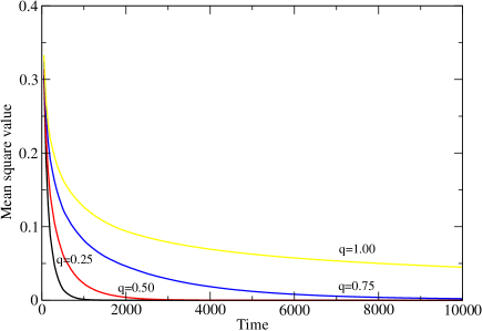
Then for a given $N$, we can vary the correlation among the noise components by varying $q\in[0:1]$ keeping fixed the noise variance. We have simulated the weight dynamics in eq. (1) by using the modification potential $\phi(y)=y(y-1)$ where we set the neuron activity $y=(\mathbf{x}\cdot\mathbf{w})/N$ to study the limit $N\gg 1$. In this simple model, if the activity $y$ is below the threshold $\theta_{m}=1$ we expect LTD and the synaptic weights $\mathbf{w}$ relax towards 0. To characterize the relaxation process, we compute the mean square value of the vector $\mathbf{w}(t)$; the results are plotted in fig. 2 for increasing values of $q$. In all cases the system (1) tends to a stationary solution. For low correlated noise we recover the equilibrium solution $\mathbf{w}=0$ as expected, but when the input noise is strongly correlated, the simulations show the existence of non zero long time persistent states for the synaptic weights. Moreover the numerical simulations suggest that the persistent states correspond to eigenvectors of the noise covariance matrix with very small eigenvalues.

Figure 2: Evolution of the norm of BCM synaptic weights when the input is the correlated noise defined by eq. (2). We consider increasing values for $q$: $q=0.25,0.50,0.75,1.00$ for $N=100$. The curves give the evolution of the mean square value of the synaptic weights $\mathbf{w}$ when the input noise correlation increases keeping the noise variance fixed (time is in arbitrary units). We note the existence of non zero long time persistent states when the correlation is high, whereas for low correlation value the system tends to the equilibrium state $\mathbf{w}=0$.

These results are consistent with experimental observationsArnold et al. (2009) on the activity of neurons in LGN in the case of monocular deprivation.

A theoretical approach linearizes the system (1) around $y\simeq 0$ by considering $\theta_{m}$ constant. Then eq. (1) becomes (cfr. fig. 1)

$$\mathbf{\dot{w}}=-\epsilon\mathbf{x}(\mathbf{w}\cdot\mathbf{x})$$ (4)

so that on average we have

$$\dot{w}_{i}=-\epsilon\sum_{j=1}^{N}C_{ij}w_{j}$$ (5)

where $C$ is the noise covariance matrix. In the case of uncorrelated input ($C_{ij}=n_{i}^{2}\delta_{ij}$ where $n_{i}^{2}$ is the $i$-component noise variance) equation (4) becomes

$$\dot{w}_{i}=-\epsilon n_{i}^{2}w_{i}$$

and $w_{i}(t)$ tends exponentially to zero with a scale time $\simeq 1/(\epsilon n_{i}^{2})$. In a generic case the system (5) can be solved by diagonalizing the covariance matrix $C$ and expand the synaptic weights $\mathbf{w}$ in the eigenvector base. Then each component $w_{\lambda}$ in this base will evolve according to

$$w_{\lambda}(t)=w_{\lambda}(0)e^{-\lambda t}$$

where $\lambda$ is the corresponding eigenvalue of the covariance matrix. As a consequence when $\lambda\ll 1$ we have long time non trivial persistent states for the synaptic weights. According to numerical simulations shown in the fig. 2 this is the case for correlated noisy input. In order to perform explicit calculations we assume that the covariance matrix is a random positive definite symmetric matrix of the form

$$C_{kl}=n^{2}(C^{0}_{kl}+mV_{kl}+O(m^{2}))$$ (6)

where

$$C^{0}=\begin{pmatrix}1&q&...&q\\ q&1&...&q\\ ..&..&...&..\\ q&q&...&1\end{pmatrix}\qquad q\leq 1$$ (7)

and $V_{kl}$ is a symmetric random matrix with zero mean value, normalized variance and i.i.d. elements. The parameter $q\in[0,1]$ determines the average correlation among the inputs and the parameter $m^{2}$ is the variance of fluctuations of the covariance matrix. The matrix (7) has the following eigenvalues

$$\lambda_{i}=\begin{cases}1+(N-1)q\qquad i=1\\ 1-q\qquad i=2,..,N\\ \end{cases}$$ (8)

Therefore when $q\to 1$ (i.e. increase of the average correlation) the eigenvalues $\lambda_{2,..,N}$ tend to 0 linearly in $(1-q)$ and the correlation matrix $C^{0}$ is degenerate. When $m=0$, the effect of correlations is to increase the decay time of $w^{(k)}$ $\propto 1/(1-q)$. In the next section we analyze the effect of fluctuations $V_{kl}$ on the eigenvalue distributions of the matrix (6) in the thermodynamics limit $N\to\infty$.

III Eigenvalue distributions

We consider the eigenvalue distributions of the matrix $C_{kl}$ (see eq. (6)) using the unperturbed covariance matrix (7). Since $C_{kl}$ is a symmetric positive definite matrix we can introduce the following representation

$$C=(\sqrt{C^{0}}+mW)^{2}=C^{0}+m(\sqrt{C^{0}}W+W\sqrt{C^{0}})+m^{2}W^{2}$$ (9)

where $\sqrt{C_{0}}$ is the symmetric square root of the matrix (7) and and $W$ is a symmetric random matrix with i.i.d. elements and zero mean value. By direct calculation we obtain the relation between $V$ and $W$

$$V=\sqrt{C^{0}}W+W\sqrt{C^{0}},$$

Then $W$ is uniquely determined as a function of $V$ and the expectation value of the covariance matrix

$$<C>=C^{0}+Nm^{2}I_{N}$$

In order to control the noise variance in the thermodynamic limit, $N\to\infty$, we introduce the scaling parameter $m_{0}$

$$m=m_{0}\sqrt{1-q\over N}$$ (10)

This is consistent with the noise definition in the numerical simulations (cfr. eq. (3)). The $\sqrt{1-q}$ dependence allows us to control the limit $q\to 1$ when the unperturbed matrix $C^{0}$ is degenerate. In real systems both $q$ and $N$ are fixed by physical conditions and $m_{0}$ is proportional to the fluctuations of the covariance matrix. In order to study the eigenvalue distribution of the covariance matrix $C$ we consider the case when $W$ is a Wigner matrixMehta (2004). Then Wigner’s theoremWigner (1958, 1967) on the eigenvalue distribution can be stated as:

Let $W_{ij}$ be a symmetric $N\times N$ random matrix with i.i.d. elements whose common distribution has zero mean value, normalized variance and is even, then the probability distribution of the eigenvalues in the interval $[\sqrt{N}\alpha,\sqrt{N}\beta]$

$$P_{N}(\sqrt{N}\alpha<\mu<\sqrt{N}\beta)\qquad-2<\alpha<\beta<2$$

is in the thermodynamics limit

$$\lim_{N\to\infty}P_{N}(\sqrt{N}\alpha<\mu<\sqrt{N}\beta)=\int_{\alpha}^{\beta}{(4-\mu^{2})^{1/2}\over 2\pi}d\lambda$$

To treat the problem of characterizing the eigenvalue distribution function when the covariance matrix $C$ has the form (9), we first perform the orthogonal transformation $O$ that diagonalizes the unperturbed matrix (7). We then restrict our analysis to the invariant subspace that corresponds to the degenerate eigenvalue $1-q$. In the thermodynamic limit the eigenvalue $1+(N-1)q$ is singular and decouples the corresponding invariant subspace. The covariance matrix (9) has the form

$$C^{\prime}=OCO^{T}=\left(\sqrt{1-q}I_{N}+m_{0}\sqrt{1-q\over N}\hat{W}\right)^{2}\qquad N\gg 1$$ (11)

where $\hat{W}=OWO^{T}$. The eigenvalue equation is

$${\rm det}\left[\lambda-\left(\sqrt{1-q}I_{N}+m_{0}\sqrt{1-q\over N}\hat{W}\right)^{2}\right]=0$$ (12)

This is equivalent to the condition

$${\rm det}[(\sqrt{N}\mu I_{N}-\hat{W})]=0$$ (13)

where we have the relation

$$\lambda=(1+m_{0}\mu)^{2}(1-q)$$ (14)

and $\mu$ are the eigenvalues of a Wigner matrix scaled by $\sqrt{N}$. As a consequence we have the following Lemma:

Any eigenvalue $\lambda$ of the matrix (11) can be written in the form (14) where $\sqrt{N}\mu$ is an eigenvalue of the Wigner matrix $W$ so that $\mu\in(-2,2)$

The relation (14) leads to the existence of two regions in the $\lambda$ spectrum according to the sign of $m_{0}\mu+1$. When $\mu>-1/m_{0}$ we invert the relation (14) by taking the positive branch of the square root

$$\mu={\sqrt{\lambda}-\sqrt{1-q}\over m_{0}\sqrt{1-q}}$$ (15)

but when $\mu<-1/m_{0}$ we have to consider the negative branch

$$\mu={-\sqrt{\lambda}-\sqrt{1-q}\over m_{0}\sqrt{1-q}}$$ (16)

The value $\mu=1/m_{0}$ is a critical value for the $\lambda$ spectrum and we expect a singularity in the eigenvalue distribution. The second case occurs only if $m_{0}>1/2$, so that there exists a critical threshold in the noise level that induces a transition in the $\lambda$ distribution. By applying Wigner’s theorem to obtain the distribution density of $\mu$ in the thermodynamic limit we obtain

$$\lim_{N\to\infty}\rho(\mu)={(4-\mu^{2})^{1/2}\over 2\pi}$$

so that in the case $m_{0}<1/2$ the distribution $\rho(\lambda)$ follows from the definition (15) according toMarchenko and Pastur (1967); Pastur (1996)

$$\rho(\lambda)=\rho(\mu){d\mu\over d\lambda}={\sqrt{4m_{0}^{2}-(\sqrt{\lambda/(1-q)}-1)^{2}}\over 4\sqrt{(1-q)\lambda}m_{0}^{2}\pi}$$ (17)

where

$$(1-q)(1-2m_{0})^{2}<\lambda<(1-q)(1+2m_{0})^{2}$$

In the case $m_{0}>1/2$ we split the $\lambda$ distribution in two parts: when

$$(1-q)(2m_{0}-1)^{2}<\lambda<(1-q)(1+2m_{0})^{2}$$

$\rho(\lambda)$ is given by eq. (17), whereas when

$$0<\lambda<(1-q)(2m_{0}-1)^{2}$$

the distribution is

$$\rho(\lambda) = {\sqrt{4m_{0}^{2}-(\sqrt{\lambda/(1-q)}-1)^{2}}\over 4\sqrt{(1-q)\lambda}m_{0}^{2}\pi}$$ (18)

$$+ {\sqrt{4m_{0}^{2}-(\sqrt{\lambda/(1-q)}+1)^{2}}\over 4\sqrt{(1-q)\lambda}m_{0}^{2}\pi}$$

In the second case the distribution is continuous for $\lambda>0$ and singular at $\lambda\to 0$. This result leads to the possibility that the correlation matrix (9) has eigenvalues arbitrarily close to zero and larger than one (corresponding to anticorrelation effects in the noise). The unperturbed correlation $q$ among the initial processes $\mathbf{x}(t)$ introduces what is essentially a scaling factor that changes the existence interval of the $\lambda$ spectrum. The critical value $m_{0}=1/2$, corresponds to a critical value of the fluctuation variance $m^{2}$ (cfr. definition (10))

$$m^{2}_{crit}={1-q\over 4N}$$ (19)

From a biophysical point of view, the results (19) implies that for sufficiently correlated noise there exist eigenvectors $w^{(k)}$ of the synaptic weights that are preserved for a very long time. This might be a possible mechanisms of maintaining synaptic weights in neuronal systems in correlated noisy environments.

IV Numerical results on finite dimension covariance matrices

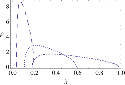
To study the effects of finite dimensions on the theoretical results (17) and (18) we have performed some numerical simulations using matrices of dimension $N=10^{3}$ that might be realistic for a neural network in LGN. In fig. 3 we show the eigenvalue distribution (17) for $m_{0}=.2$ and different values of the correlation ($q=.5,.7,.9$).

Figure 3: Plots of eigenvalue distributions $\rho(\lambda)$ (see definition (17)) for the correlation matrix (3) using $m_{0}=.2$ and $q=.5,.7,.9$ respectively the dashed-dotted, the dotted and the dashed line. As the average correlation $q$ increases the eigenvalue spectrum is squeezed towards the origin.

To see the effect of the transition in the distribution function at the critical value (19), we computed the eigenvalues distribution in the cases $q=.5$ and $m_{0}=.4,.6,.8$. The results are shown in fig. 4

Figure 4: Plot of the eigenvalue distribution for the correlation matrix (3) using $q=.5$ and $m_{0}=.2,.4,.6,.8$ from left to right and top to bottom. The effect of the transition at the critical value $m_{0}=.5$ is clearly seen: the eigenvalues accumulate at the origin. The continuous line is the theoretical distribution (17) whereas the histograms are numerically computed using a random matrix of order $N=10^{3}$.

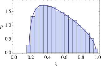
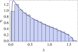
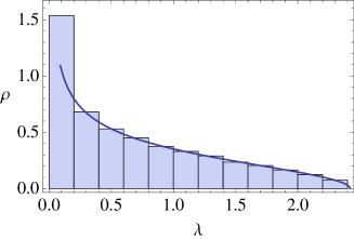
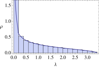
We observe, as in the case of low correlation, the eigenvalue distributions become larger than in the correlated case and have values beyond 1 when $m_{0}$ increases. When $m_{0}\to 1/2$ the distribution becomes singular and the distribution peak tends to zero, so that there exist eigenvectors $w^{(k)}$ with extremely long decay times in eq. (4).

V Generalization to a neural network

For a network of neurons, eq. (1) can be generalized Castellani et al. (1999) to

$$\mathbf{\dot{w}}^{(k)}=\mathbf{x}^{(k)}\phi(y^{(k)},\theta_{m}^{(k)})\qquad k=1,...,N$$ (20)

where the index $k$ refers to the $k$-th neuron of the network and $N$ is the number of neurons. We then have

$$y^{(k)}=\mathbf{x}^{(k)}\cdot\mathbf{w}^{(k)}+\sum_{l=1}^{N}L_{kl}y^{(l)}$$ (21)

where we have introduced lateral connections, $L$, among the neurons. We can have both excitatory or inhibitory neural connections according to the sign of $L_{kl}$. In what follows we assume that $L$ is a symmetric matrix with $\|L\|\ll 1$ where $\|\quad\|$ denotes the usual matrix norm. Therefore the neurons form a bidirectional symmetric network; we can invert the relation (21) to obtain

$$y^{(k)}=\sum_{l=1}^{N}(I-L)^{-1}_{kl}\mathbf{x}^{(l)}\cdot\mathbf{w}^{(l)}$$ (22)

For monocular deprivation eq. (21) becomes a network generalization of eq. (4)

$$\mathbf{\dot{w}}^{(k)}=-\epsilon^{(k)}\mathbf{x}^{(k)}y^{(k)}\qquad k=1,...,N$$ (23)

where $\epsilon^{(k)}$ are suitable positive constants. By substituting eq. (22) into (23), we get the linear system

$$\mathbf{\dot{w}}^{(k)}=-\epsilon^{(k)}\mathbf{x}^{(k)}\sum_{l=1}^{N}(I-L)^{-1}_{kl}\mathbf{x}^{(l)}\cdot\mathbf{w}^{(l)}\qquad k=1,...,N$$ (24)

In what follows we regard the inter-neuron connections $L$, as not-modifiable. Moreover for simplicity we reduce external input to one dimension for each neuron: then both $\mathbf{w}^{(k)}$ and $\mathbf{x}^{(k)}$ are scalar. In order to study the dynamical properties of the solutions we average on fast scale variations of the noise; the equations (24) become

$$\dot{w}^{(k)}=-\epsilon^{(k)}\sum_{l=1}^{N}(I-L)^{-1}_{kl}C_{kl}w^{(l)}\qquad k=1,...,N$$ (25)

where $C_{kl}$ is the noise covariance matrix between the inputs of the $k$ and $l$ neuron. We consider the connection matrix $L$ as a symmetric random matrix, so that according to our hypotheses the matrix $(I-L)^{-1}$ is a symmetric positive definite matrix. Then (25) can be written in the form

$$\dot{w}^{(k)}=-\epsilon^{(k)}\sum_{l=1}^{N}\hat{L}_{kl}w^{(l)}\qquad k=1,...,N$$ (26)

where

$$\hat{L}_{kl}=(I-L)^{-1}_{kl}C_{kl}$$ (27)

is still a symmetric positive definite matrix. If the input signals are independent ($C_{kl}=\sigma_{k}^{2}\delta_{kl}$), we obtain

$$\dot{w}^{(k)}=-\epsilon^{(k)}n_{k}^{2}(I-L)^{-1}_{kk}w^{(k)}\qquad k=1,...,N$$

and the $w^{(k)}$ exponentially decay towards zero. Again the interesting case is when the covariance matrix is not diagonal and the connections $L$ are defined by a random matrix; from a biological point of view we are modeling a ensemble of neurons which are stimulated by correlated inputs and have bilateral connections with random weights. When $\hat{L}$ has the form (cfr. eq. (6))

$$\hat{L}_{kl}=C^{0}_{kl}+mV_{kl}+O(m^{2})$$ (28)

we can apply the method used for a single neuron to study the eigenvalue distribution. But in the network case we have a new biophysical interpretation of the critical value (19): if number of neurons is sufficiently large and/or the fluctuations in the bilateral neural connections exceed a threshold, the network is able to develop $w^{(k)}$ eigenvectors with extremely long lifetimes in presence of a noisy correlated input. This phenomenon suggests mechanisms for long network lifetimes in noisy environments. The possibility that correlated noise plays a role in the dynamics of a neural network has been investigated in Glatt et al. (2006) using different models.

VI Conclusions

We have analyzed the effects of noise correlations in the input to, or among, BCM neurons using the Wigner semicircular law to construct random, positive-definite symmetric correlation matrices and computing their eigenvalue distributions. In the finite dimensional case, our analytic results are compared with numerical simulations. We thus show the effects of correlations on the lifetimes of the synaptic strengths in various visual environments. In the case of a single neuron the noise correlations arise from the input LGN neurons, whereas the correlations arise also from the lateral connections in a neuron network. If the dimensionality of system is fixed, we show that when the fluctuations of the covariance matrix exceed a critical threshold synapses with long lifetimes arise. These results may be of physiological significance and can be tested experimentally.

References

- Bear and Rittenhouse (1999) M. F. Bear and C. D. Rittenhouse, J Neurobiol 41(1), 83 (1999).
- Sengpiel and Kind (2002) F. Sengpiel and P. C. Kind, Curr Biol 12(23), R818 (2002).
- Blais et al. (1998) B. S. Blais, N. Intrator, H. Shouval, and L. N. Cooper, Proceedings of the National Academy of Sciences 10(7), 1797 (1998).
- Cooper et al. (2004) L. N. Cooper, N. Intrator, B. S. Blais, and H. Z. Shouval, Theory of cortical plasticity (World Scientific New Jersey, 2004).
- Wiesel and Hubel (1962) T. Wiesel and D. Hubel, Journal of Physiology 180, 106 (1962).
- Rittenhouse et al. (1999) C. D. Rittenhouse, H. Z. Shouval, M. A. Paradiso, and M. F. Bear, Nature 397, 347 (1999).
- Frenkel and Bear (2004) M. Y. Frenkel and M. F. Bear, Neuron 44, 917 (2004).
- Bienenstock et al. (1982) E. L. Bienenstock, L. N. Cooper, and P. W. Munro, Journal of Neuroscience 2, 32 (1982).
- Whitlockand et al. (2006) J. R. Whitlockand, A. J. Heynen, M. G. S. MG, and M. F. Bear, Science 313, 1093 (2006).
- Castellani et al. (2001) G. C. Castellani, E. M. Quinlan, L. N. Cooper, and H. Z. Shouval, Proceedings of the National Academy of Sciences 98(22), 12772 (2001).
- Abbott and B.Nelson (2000) L. F. Abbott and S. B.Nelson, Nature Neuroscience 3, 1178 (2000).
- Gerstner et al. (1996) W. Gerstner, R. Kempter, J. L. van Hemmen, and H. Wagner, Nature 383, 76 (1996).
- Gerstner and Kistler (2002) W. Gerstner and W. M. Kistler, Biological Cybernetics 87, 404 (2002).
- Arnold et al. (2009) M. L. Arnold, J. Heynen, R. H. Haslinger, and M. F. Bear, Nature Neuroscience 12, 390 (2009).
- Weliky and Katz (1999) M. Weliky and L. C. Katz, Science 285, 599 (1999).
- Ohshiro and Weliky (2006) T. Ohshiro and M. Weliky, Nat Neurosci 9(12), 1541 (2006).
- (17) B. S. Blais, L. N. Cooper, and H. Shouval, Effect of correlated lgn firing rates on predictions for monocular eye closure vs monocular retinal inactivation, eprint submitted for publication.
- Bazzani et al. (2003) A. Bazzani, D. Remondini, N. Intrator, and G. C. Castellani, Neural Computation 15(7), 1621 (2003).
- Wigner (1958) E. P. Wigner, The Annals of Mathematics 67-2, 325 (1958).
- Wigner (1967) E. P. Wigner, SIAM Review 9, 1 (1967).
- Mehta (2004) M. L. Mehta, Random Matrices, vol. 142 (Elsevier Pure and Applied Mathematics, 2004).
- Marchenko and Pastur (1967) V. Marchenko and L. Pastur, Mat. Sb. 72, 507 (1967).
- Pastur (1996) L. A. Pastur, Annales de l’I.H.P. section A 64, 325 (1996).
- Castellani et al. (1999) G. C. Castellani, N. Intrator, H. Shouval, and L. N. Cooper, Networks :Comput. Neur. Syst. 10, 111 (1999).
- Glatt et al. (2006) E. Glatt, H. Busch, F. Kaiser, and A. Zaikin, Phys. Rev. E 73, 026216 (2006).