Seven-Year Wilkinson Microwave Anisotropy Probe (WMAP11affiliation: WMAP is the result of a partnership between Princeton University and NASA’s Goddard Space Flight Center. Scientific guidance is provided by the WMAP Science Team. ) Observations: Power Spectra and WMAP-Derived Parameters
Abstract
The WMAP mission has produced sky maps from 7 years of observations at L2. We present the angular power spectra derived from the 7-year maps and discuss the cosmological conclusions that can be inferred from WMAP data alone.
With the 7-year data, the temperature (TT) spectrum measurement has a signal-to-noise ratio per multipole that exceeds unity for ; and in band-powers of width , the signal-to-noise ratio exceeds unity up to . The third acoustic peak in the TT spectrum is now well measured by WMAP. In the context of a flat model, this improvement allows us to place tighter constraints on the matter density from WMAP data alone, , and on the epoch of matter-radiation equality, . The temperature-polarization (TE) spectrum is detected in the 7-year data with a significance of , compared to with the 5-year data. We now detect the second dip in the TE spectrum near with high confidence. The TB and EB spectra remain consistent with zero, thus demonstrating low systematic errors and foreground residuals in the data. The low- EE spectrum, a measure of the optical depth due to reionization, is detected at significance when averaged over –7: K2 (68% CL). We now detect the high-, , EE spectrum at over 8 . The BB spectrum, an important probe of gravitational waves from inflation, remains consistent with zero; when averaged over –7, K2 (95% CL). The upper limit on tensor modes from polarization data alone is a factor of 2 lower with the 7-year data than it was using the 5-year data (Komatsu et al., 2010).
The data remain consistent with the simple model: the best-fit TT spectrum has an effective of 1227 for 1170 degrees of freedom, with a probability to exceed of 9.6%. The allowable volume in the 6-dimensional space of parameters has been reduced by a factor of 1.5 relative to the 5-year volume, while the model that allows for tensor modes and a running scalar spectral index has a factor of 3 lower volume when fit to the 7-year data. We test the parameter recovery process for bias and find that the scalar spectral index, , is biased high, but only by 0.09 , while the remaining parameters are biased by .
The improvement in the third peak measurement leads to tighter lower limits from WMAP on the number of relativistic degrees of freedom (e.g., neutrinos) in the early universe: . Also, using WMAP data alone, the primordial helium mass fraction is found to be , and with data from higher-resolution CMB experiments included, we now establish the existence of pre-stellar helium at (Komatsu et al., 2010). These new WMAP measurements provide important tests of Big Bang cosmology.
1. INTRODUCTION
The Wilkinson Microwave Anisotropy Probe (WMAP Bennett et al., 2003b, a) is a Medium-Class Explorer (MIDEX) satellite aimed at understanding cosmology through full-sky observations of the cosmic microwave background (CMB). The WMAP full-sky maps of the temperature and polarization anisotropy in five frequency bands provide our most accurate view to date of conditions in the early universe. The WMAP instrument is composed of 10 differencing assemblies (DAs) spanning 5 frequencies from 23 to 94 GHz (Bennett et al., 2003b): one DA each at 23 GHz (K1) and 33 GHz (Ka1), two each at 41 GHz (Q1,Q2) and 61 GHz (V1,V2), and four at 94 GHz (W1–W4). Each DA is formed from two differential radiometers which are sensitive to orthogonal linear polarization modes; WMAP measures both temperature and polarization at each frequency. The multi-frequency data facilitate the separation of the CMB signal from foreground emission arising both from our Galaxy and from extragalactic sources. The CMB angular power spectrum derived from these maps exhibits a highly coherent acoustic peak structure which makes it possible to extract a wealth of information about the composition and history of the universe, as well as the processes that seeded the fluctuations.
With accurate measurements of the first few peaks in the angular power spectrum, CMB data have enabled the following advances in our understanding of cosmology (Spergel et al., 2003, 2007; Dunkley et al., 2009; Komatsu et al., 2009): the dark matter must be non-baryonic and interact only weakly with atoms and radiation; the density of atoms in the universe is known to 3%, and accords well with Big Bang Nucleosynthesis; the measured acoustic scale at , combined with the local distance scale and Baryon Acoustic Oscillation (BAO) data, demonstrates that the universe is spatially flat, to within 1%; the Hubble constant is determined to 3% using only acoustic fluctuation data (CMB+BAO), and it accords well with local measurements; the primordial fluctuations are adiabatic and Gaussian, and the spectrum is slightly tilted.
The statistical properties of the CMB fluctuations measured by WMAP are close to Gaussian with random phase (Komatsu et al., 2003; Spergel et al., 2007; Komatsu et al., 2009). There are several hints of possible deviations from this case as discussed in Bennett et al. (2010); Komatsu et al. (2010). If the fluctuations are Gaussian and random phase, then their statistical information content is completely determined by the angular power spectra of the sky maps.
This paper derives the angular power spectra from the WMAP 7-year sky maps and presents the cosmological parameters that can be determined from them. The new results improve upon previous results in many ways: additional data reduces the random noise, which is especially important for studying the temperature signal on small angular scales and the polarization signal on large angular scales; W band data is now incorporated in the TE spectrum measurement to improve precision; new simulations have been carried out to test the accuracy of parameter recovery and to test a model’s goodness of fit. The result is the most accurate full sky measurement to date of CMB anisotropy down to an angular scale of .
This paper is one of six that accompany the 7-year WMAP data release. Jarosik et al. (2010) discuss the 7-year map making process, systematic error limits, and basic results. Gold et al. (2010) discuss galactic foreground emission, and its removal in 7-year data. Bennett et al. (2010) discuss possible anomalies in the WMAP CMB maps. Komatsu et al. (2010) discuss the interpretation of the WMAP data, in combination with other relevant cosmological data. Weiland et al. (2010) discuss the WMAP measurements of the outer planets and selected bright sources for use as microwave calibrators.
The layout of this paper is as follows. In §2, we present the WMAP 7-year power spectra. In §3, we discuss simulations that were performed to test for bias in our cosmological parameter fits. In §4 we discuss cosmological conclusions that can be drawn from WMAP data alone, and in §5 we discuss the goodness of fit of the 6-parameter theory. We conclude in §6.
2. SEVEN-YEAR POWER SPECTRA
In this section we present the temperature and polarization power spectra derived from the 7-year sky maps and compare them to the 5-year spectra.
2.1. Definitions and Methodology
Since WMAP measures both temperature and polarization, there are multiple power spectra to consider. On a sphere, the temperature field can be decomposed into spherical harmonics,
| (1) |
where is a unit direction vector and refers specifically to the temperature field. Likewise, the Q and U Stokes parameters for linear polarization can be decomposed into complex spin-2 harmonics (Newman & Penrose, 1966; Goldberg et al., 1967),
| (2) |
The spin-2 coefficients can then be combined to represent polarization modes that have no curl (E modes) and modes that have no divergence (B modes). These are given by the coefficients (Zaldarriaga & Seljak, 1997; Larson, 2006),
| (3) | |||||
| (4) |
(Kamionkowski et al. (1997) use an alternative approach.) The angular power spectra are related to these modes according to
| (5) |
where X, Y = T, E, or B. The data are currently consistent with being isotropic and Gaussian distributed, but this condition should continue to be tested (Bennett et al., 2010).
There are 6 independent power spectra than can be constructed from the temperature and polarization data, TT, TE, TB, EE, EB, and BB, though in theories in which parity is conserved, TB and EB are expected to be zero. In general, foreground signals (and systematic effects) can produce non-zero TB, EB, and BB so these spectra provide a good test for residual polarization contamination.
For the 7-year analysis, we use the same combination of estimators that were used with the 5-year data (Nolta et al., 2009). This combination is a trade-off between statistical accuracy and computational speed. We present new tests of the accuracy of the likelihood function constructed from these estimators in §3. To summarize the combination: for low- TT () we compute the likelihood of a model directly from the 7-year Internal Linear Combination (ILC) maps (Gold et al., 2010). For high- () TT we use the MASTER pseudo- quadratic estimator (Hivon et al., 2002). For low- polarization, TE, EE, & BB, we use the pixel-space estimator described in Page et al. (2007), and for high- TE () we use the MASTER quadratic estimator.
2.2. Changes Affecting the 7-Year Spectra
Several data processing and analysis changes were applied to the 7-year data which resulted in improvements beyond those which would be expected from additional integration time.
2.2.1 Map-Making with Asymmetric Masking
A new map-making technique was adopted for the 7-year data which combines optimal noise handling with “asymmetric” data masking (Jarosik et al., 2010). With this change, certain regions in the 7-year maps employ more data samples than they would have with the previous pipeline. These “Galactic echo” regions are thus more sensitive than a simple 5-year to 7-year integration time scaling would predict.
2.2.2 Multipole Range
The additional sensitivity afforded by more data has made it possible to extend the usable multipole range in the power spectra and likelihood code. For the TT data we extend the upper multipole limit, , from 1000 to 1200. For the TE spectrum, we have determined that high- W-band polarization data are sufficiently free from systematic effects that they can be employed in the TE spectrum estimate (Jarosik et al., 2010). This significantly improves the sensitivity in the 7-year TE spectrum and allows us to extend the TE multipole limit from 450 to 800.
2.2.3 Mask and
The 7-year sky masks have been augmented slightly using a analysis of the Q–V & V–W difference maps, after the normal template cleaning had been applied (Jarosik et al., 2010; Gold et al., 2010). This results in a slightly more conservative mask which decreases the unmasked sky fraction by % (from 81.7% to 78.3% for the KQ85 cut—the new cut is denoted KQ85y7). Given the threshold applied during the construction of the extended mask, residual foreground signals outside the mask are essentially undetectable on the scale of the instrument noise in a 2∘ pixel, so the data are fractionally more robust to foreground contamination.
The power spectrum sensitivity depends on sky cut according to where is (approximately) the fraction of sky that survives the cut (Hinshaw et al., 2003; Verde et al., 2003). In practice, is a function of that is calibrated with simulations, so there is a different constant of proportionality at each , but it scales with the fraction of usable sky area. Thus the increased sky mask results in a slight loss of sensitivity in the TT spectrum for , where the spectrum is sky variance limited.
For the TE spectrum, we have generated new simulations to test the calibration of which enters into the error propagation from sky maps to spectra. The mean deduced from our simulations was 760 for spectra with 777 degrees of freedom, a factor of 1.022 too low, indicating that our previous TE error estimate was a factor of 1.011 too high. Therefore we have scaled by 1.011 to produce a unit mean per degree of freedom, following the precedent used to calibrate from simulations (Verde et al., 2003). In §5 we present the TE of the 7-year flight data and conclude that the model fits the TE data well.
2.3. Temperature (TT) Spectrum
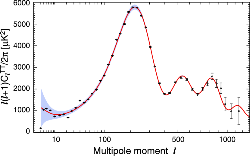
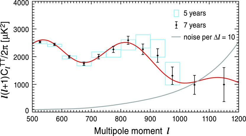
For , the spectrum is obtained using a Blackwell-Rao estimator applied to a chain of Gibbs samples (Wandelt et al., 2004; Jewell et al., 2004; Chu et al., 2005; Dunkley et al., 2009) based on the 7-year ILC map and the KQ85y7 mask. The specifications used to sample the map are described in Dunkley et al. (2009). For , the spectrum was derived from the MASTER pseudo- quadratic estimator applied to the 7-year, template-cleaned V and W-band maps (Gold et al., 2010). (The MASTER spectrum is technically derived from to 1200, then the portion is discarded, but correlations induced by mode coupling are retained for .) The pseudo- coefficients were computed from the maps for each single year and each single-DA, V1-W4. For the coefficients were evaluated with uniform pixel weights, while inverse-noise weights were used for . (The transition was made at in the 5-year analysis.) As noted above, we adopt a slightly larger sky mask, denoted KQ85y7.
The pseudo- cross-power spectra are computed from all off-diagonal pairs of pseudo- coefficients,
| (6) |
where , refer to a DA-year combination (Hinshaw et al., 2007) and the tilde indicates a pseudo-quantity (spectrum or coefficient). These component pseudo-spectra are deconvolved using the MASTER formalism111 In principle, we can obtain a modestly more sensitive spectrum estimate at intermediate multipoles by employing weighting in the computation of the pseudo-. We are currently developing such code for use in cross-power spectra with the intention of applying it to the final 9-year data., and the results are combined by band into VV, VW, and WW spectra for the purposes of removing the residual point source amplitude. The unresolved point source contribution to the sky continues to be treated as a power law in thermodynamic temperature, falling as (Nolta et al., 2009), but see Colombo & Pierpaoli (2010) for an alternative approach to the spectral dependence. Using the same fitting methodology as in the 5-year analysis, we find its amplitude to be , when fit to the 7-year Q, V, and W band spectra evaluated with the KQ85y7 mask. (Most of the cosmological parameters reported in this paper were fit using a preliminary version of the likelihood that had a small masking error that produced a slightly biased TT spectrum at high- and a correspondingly higher residual source amplitude, which mostly compensated for the bias. We have checked that substituting the correct TT spectrum has a negligible effect on the parameter fits.) After this source model is subtracted from each band, the spectra are combined to form our best estimate of the CMB signal, shown in Figure 1.
The 7-year power spectrum is cosmic variance limited, i.e., cosmic variance exceeds the instrument noise, up to . (This limit is slightly model dependent and can vary by a few multipoles.) The spectrum has a signal-to-noise ratio greater than one per -mode up to , and in band-powers of width , the signal-to-noise ratio exceeds unity up to . The largest improvement in the 7-year spectrum occurs at multipoles where the uncertainty is still dominated by instrument noise. The instrument noise level in the 7-year spectrum is 39% smaller than with the 5-year data, which makes it worthwhile to extend the WMAP spectrum estimate up to for the first time. See Figure 2 for a comparison of the 7-year error bars to the 5-year error bars. The third acoustic peak is now well measured and the onset of the Silk damping tail is also clearly seen by WMAP. As we show in §4, this leads to a better measurement of and the epoch of matter-radiation equality, , which, in turn, leads to better constraints on the effective number of relativistic species, , and on the primordial helium abundance, . The improved sensitivity at high is also important for higher-resolution CMB experiments that use WMAP as a primary calibration source.
2.4. Temperature-Polarization (TE, TB) Cross Spectra
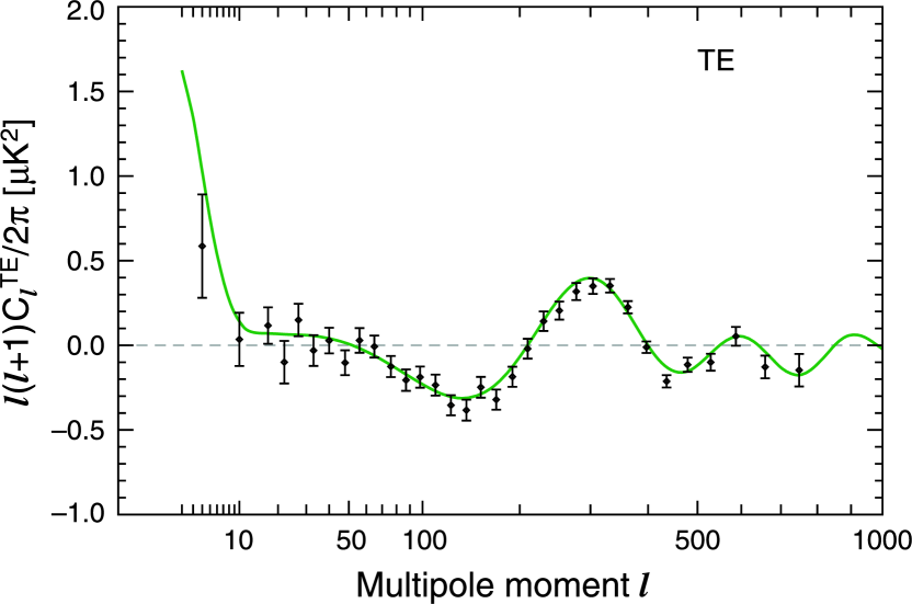
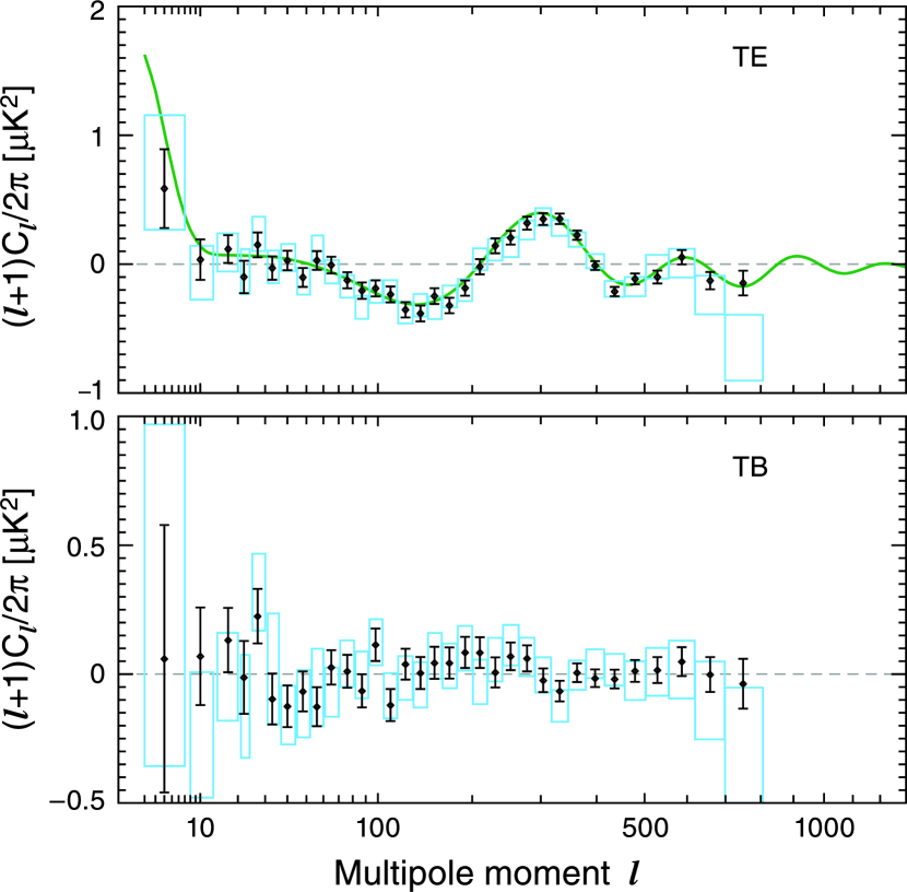
The 7-year temperature-polarization cross power spectra were formed using the same methodology as the 5-year spectrum (Page et al., 2007; Nolta et al., 2009). For the cosmological model likelihood is estimated directly from low-resolution temperature and polarization maps. The temperature input is a template-cleaned, co-added V+W band map, while the polarization input is a template-cleaned, co-added Ka+Q+V band map (Gold et al., 2009). In this regime, the spectrum can be inferred from the conditional likelihood of values (individual or binned), but these estimates are only used for visualization.
For , the temperature-polarization spectra are derived using the MASTER quadratic estimator, extended to include polarization data (Page et al., 2007). (As above, the MASTER spectrum is evaluated from , but the result from is discarded.) The temperature input is a template-cleaned, co-added V+W band map, while the polarization input is a template-cleaned, co-added Q+V+W band map. The inclusion of W-band data in the high- TE and TB spectra is new with the 7-year data release (Jarosik et al., 2010). Since the W band radiometers have the highest angular resolution, the inclusion of W band significantly enhances the sensitivity of these high- spectra.
The 7-year TE spectrum measured by WMAP is shown in Figure 3. For all except the first bin, the MASTER values and their Gaussian errors are plotted. The first bin shows the conditional maximum likelihood value based on the pixel likelihood mentioned above. The slight adjustment for is included in the error bars. With two additional years of integration and the inclusion of W band data, we now detect the TE signal with a significance of 20, up from 13 with the 5-year data. Indeed, for , the TE error is less than 65% of the 5-year value, and for the sensitivity improvement is even larger due to W band’s finer resolution. At the 7-year TE error is 36% of the 5-year value. A qualitatively new feature seen in the 7-year spectrum is a second trough (TE0) near . See Figure 4 for a comparison of the 7-year to 5-year error bars, for the TE and TB spectra. Overall, the TE data are quite consistent with the simplest 6-parameter model; we discuss its goodness-of-fit in §5.
The observed TE signal is the result of a specific polarization pattern around hot and cold spots in the temperature anisotropy. In particular, the acoustic peak structure in TE corresponds to a series of concentric rings of alternating radial and tangential polarization (relative to a radial reference direction). Komatsu et al. (2010) perform a stacking analysis of the 7-year temperature and polarization maps and show that the effect is detected in the 7-year WMAP sky maps with a significance of 8.
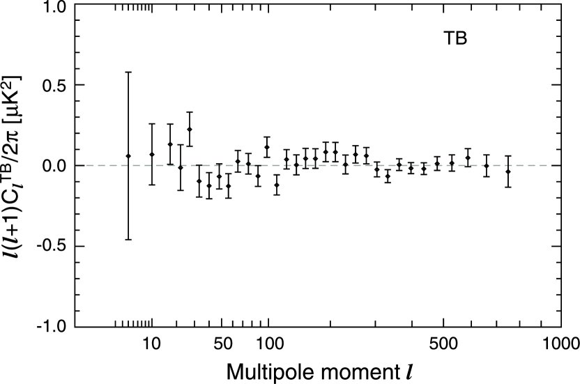
The 7-year TB spectrum measured by WMAP is shown in Figure 5. In this case, because the signal-to-noise ratio is low, the MASTER points and their Gaussian errors are plotted over the full range, including the first bin. The measured spectrum is consistent with zero: the for the null hypothesis (TB=0) is 793.5 for 777 degrees of freedom. The probability to exceed that amount is 33%. The absence of a detectable signal is consistent with the model, which predicts zero. It is also an indication that systematic errors and foreground contamination are not significant at the level of K2 in .
Komatsu et al. (2010) use the 7-year TE and TB data to place limits on polarization rotation due to parity violating effects. Polarization rotation would cause TE signal generated at the last scattering surface to transform into observed TB power. The absence of TB signal leads to an upper limit on rotation of .
2.5. Polarization (EE, EB, BB) Spectra
We begin by discussing the low- polarization spectra, and then move on to the high- EE spectrum.
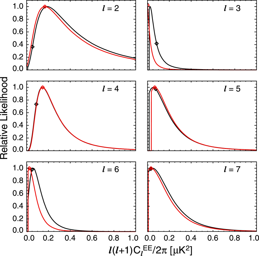
The most reliable way to estimate the low- polarization spectra is to use the pixel-space likelihood code to generate the posterior distributions of individual (or binned) values. In the 7-year data, this code is based on a co-added Ka+Q+V map. The most conservative, but costly, method is to produce a Markov Chain that allows each to vary independently; the resulting distribution of any single will be the marginalized distribution for that multipole moment. A Gibbs sampling technique could also be used, but this works best with a high signal-to-noise ratio. However, Gibbs sampling in lower signal-to-noise regions can be performed successfully, as shown by Jewell et al. (2009). A much more tractable approach is to compute the conditional likelihood in which the likelihood of a single is evaluated while all other moments are held fixed. We adopt the latter approach to visualize the low- EE and BB spectra. This method has also been used in previous WMAP papers as well as (for example) Gruppuso et al. (2009) in their verification of the 5-year WMAP low- spectra. In the context of parameter fitting, the estimated are constrained to vary according to the model.
Figure 6 shows the conditional likelihood for the EE multipoles from –7 for two different reference spectra. The black curves show the likelihood of when the are fixed to the best-fit model for . The red curves are the analogous distributions when the reference spectrum is taken to be the maximum likelihood spectrum. This maximum likelihood spectrum was obtained by numerical maximization of the likelihood code for the TT, TE, EE, and BB spectra for , a maximization in 36 dimensions, while the spectra at were fixed at the best-fit model. Save for and 6, the likelihood curves are relatively insensitive to the difference between these two reference spectra. From these curves it is clear that the majority of the statistical weight in the low- EE detection is at , with also contributing significant power.
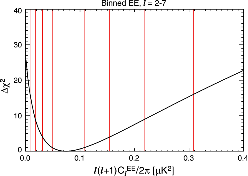
A standard reionization scenario would give rise to a relatively flat spectrum in over the range , so it is of interest to evaluate the posterior distribution of a band power with constant over this range. As shown in Figure 7, we find
| (7) |
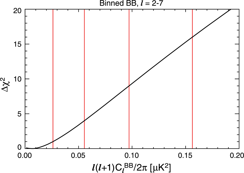
This result was obtained with the pixel likelihood code, and so the error bars include cosmic variance. Additionally, a model with zero TE and EE power for = 2–7 is disfavored at 5.5 relative to the most-likely constant band-power in this range.
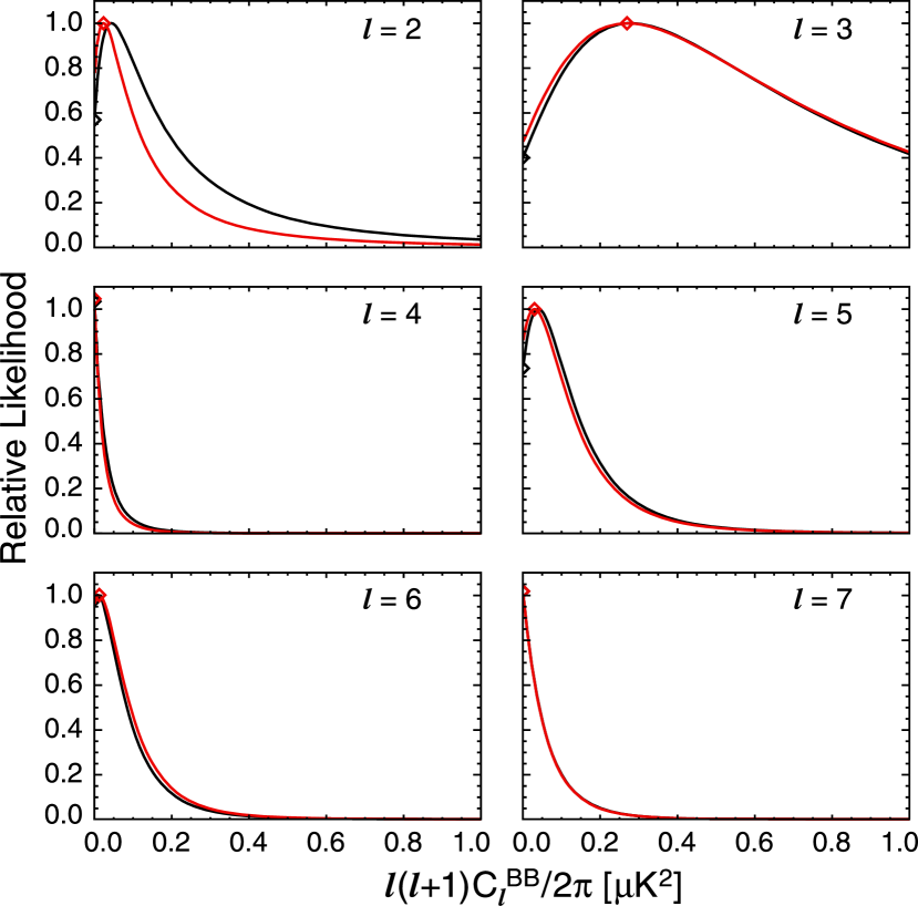
Figure 8 shows the conditional likelihood for the BB multipoles from –7 for two different reference spectra. The black curves show the likelihood of when the are fixed to the best fit model (zero, except for small contributions from lensing) for . The red curves are the analogous distributions when the reference spectrum is taken to be the maximum likelihood spectrum for and the spectrum (again, effectively zero) for . Save for , the posterior likelihood curves are insensitive to the reference spectrum. There is no significant detection of BB power in any single multipole in the 7-year WMAP data. As shown in Figure 9, we evaluate the posterior likelihood of a single constant band-power from and find it is also consistent with zero. We place an upper limit of
| (8) |
using the 7-year WMAP data, which is more than a factor of 2 lower than the 5-year limit of 0.15 K2.
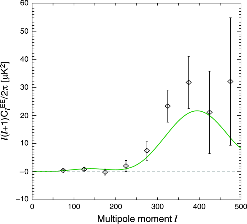
The high- EE spectrum is constructed using the polarized spectra that were used for the TE spectrum, discussed in §2.4. Figure 10 plots the 7-year WMAP data on top of the EE spectrum that best fits the WMAP data. Note that the high- EE spectrum is not included in the likelihood code, so the theory curve is not a best fit to the high- EE spectrum.
Using error bars with cosmic variance derived from the best fit model, we find , for the 777 degrees of freedom in the multipole range . The probability to exceed this value is 8.9%, which is low, but not significantly so. For a model with no EE spectrum, . The difference is , which is just over an 8 detection of the high- EE spectrum.
The data prefer an EE spectrum with higher amplitude than the best-fit model. To quantify this, we find the scale factor that causes the theory EE spectrum to best fit the data, over the multipole range . The scale factor is . This indicates a 2.5 preference for a higher amplitude EE spectrum, which we consider to be worth further investigation, but do not believe to be a significant deviation from the theory. Note that other experiments, such as QUaD (Brown et al., 2009), find the EE spectrum to be consistent with the prediction of the best-fit model.
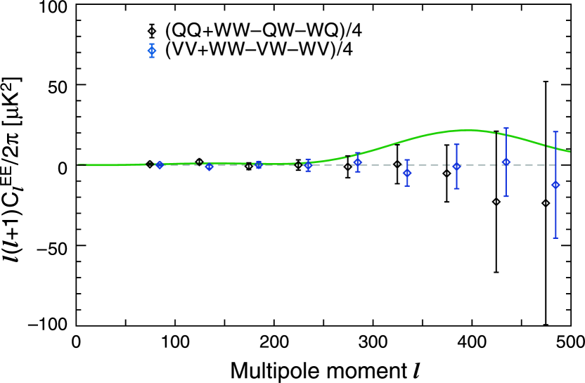
To verify that we are not seeing the power spectrum in just one band and not the others, we take difference spectra among the Q, V, and W bands. Figure 11 shows two sets of difference spectra. These spectra are consistent with zero, as expected, and demonstrate that the EE power spectrum is present in all three frequency bands.
2.6. WMAP Likelihood Code
Before discussing cosmological parameter fits in the remainder of the paper, we review the WMAP likelihood code which forms the basis for the fits.
The basic structure of the likelihood code is unchanged from the 5-year release. For the temperature data, the model spectrum is compared to the MASTER spectrum, described above, using a Gaussian plus log-normal approximation to the likelihood, as described in Bond et al. (1998) and Verde et al. (2003). For a Blackwell-Rao estimator is used to determine the likelihood of a model TT spectrum (Dunkley et al., 2009). This estimator encodes both the low- spectrum and an accurate description of its non-Gaussian errors. It is constructed from a set of Gibbs samples that contain power spectra and CMB maps that are statistically consistent with the data (Wandelt et al., 2004; Jewell et al., 2004; Eriksen et al., 2004). The 7-year input to the Gibbs chain mimics the 5-year input: we smooth the Internal Linear Combination (ILC) map to 5∘ (Gaussian FWHM); degrade it to resolution ; and add Gaussian white noise with 2 K to each pixel. The data are masked with the KQ85y7 mask degraded to , and the Gibbs sampler is run to produce input for the Blackwell-Rao estimator; further details are given in Dunkley et al. (2009).
For the polarization data, we use a similar hybrid scheme: for the TE data we compare a model spectrum to the MASTER spectrum using a Gaussian likelihood. (TE is the only high- polarization data used in the WMAP likelihood code.) For , the likelihood of model TE, EE, and BB spectra are obtained using a pixel-space likelihood which is based on the map mentioned in §2.4 and described in (Page et al., 2007).
The likelihood code includes several important factors: mode coupling due to sky masking and non-uniform pixel weighting (due to non-uniform noise); beam window function uncertainty, which is correlated across the entire spectrum; and residual point source subtraction uncertainty, which is also highly correlated. The treatment of these effects is unchanged from the 5-year analysis (Nolta et al., 2009; Dunkley et al., 2009).
Note added in revision—The results in this paper were prepared using version 4.0 of the WMAP likelihood. Since the initial submission of this paper, two small errors in the likelihood code came to light. 1) The original computation of the TT spectrum used an incorrect monopole subtraction which resulted in a small amount of excess power at high , and a corresponding elevation of the best-fit residual point source amplitude. Correcting the monopole subtraction reduced the high- power slightly which produced a correspondingly lower residual point source amplitude, from to K2 sr. 2) Due to a simulation configuration error, the TE recalibration factor used in version 4.0 was 3.8% larger than the final value reported in §2.2.3. The first of these changes will not affect the simulations in §3, because they lack a monopole, and the new value for TE has been used for the §3 parameter recovery simulations. The goodness of fit statistics for the TT and TE spectra in §5 compare the best fit theory spectrum from the version 4.0 Markov chains (with RECFAST version 1.4.2) to the version 4.1 likelihood data. See Appendix B for a comparison of parameters, when estimated with the original and updated versions of the code.
2.6.1 CAMB
For computing theoretical power spectra, we use the Code for Anisotropies in the Microwave Background (CAMB) (Lewis et al., 2000) which is based on the earlier code CMBFAST (Seljak & Zaldarriaga, 1996).222We use the November 2008 version of CAMB, which was updated to remove a bug affecting lensed non-flat models in February 2009. The update was inadvertently not included in our current analysis, but we have checked that the effect on spectra is at the sub-percent level. Since 2008 the CAMB package has supported improved modeling of reionization, as follows: 1) inclusion of helium reionization, assuming that helium is singly reionized at the same time as hydrogen and doubly reionized at (this slightly lowers the redshift of reionization for a given optical depth); 2) the width of reionization can be varied without changing the optical depth. We use a width as standard. Seven-year reionization results are discussed in §4.2.7.
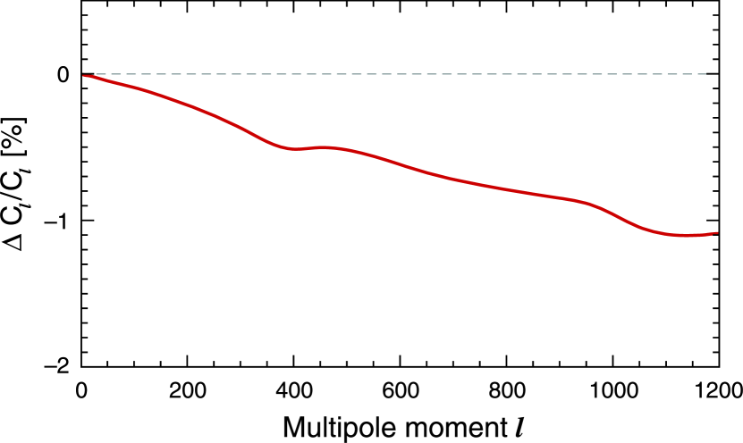
Shortly after the 7-year WMAP data were released, a new version of CAMB was made available, incorporating an updated version of the code used to model recombination: RECFAST (Seager et al., 1999, 2000; Wong et al., 2008; Scott & Moss, 2009). The parameter recovery was run with RECFAST version 1.4.2, and the January 2010 version of CAMB updates this to RECFAST version 1.5. The primary change is in the optical depth, due to more accurate modeling of the physics of the hydrogen atom. Figure 12 shows how much the new version of RECFAST lowers the power spectrum, for a given set of cosmological parameters. The fractional lowering is largest at high and is about 1% at .
3. PARAMETER RECOVERY BIAS TESTS
| Parameter | Description |
|---|---|
| Fit parameters | |
| Physical baryon density | |
| Physical cold dark matter density | |
| Dark energy density ( unless otherwise noted - see below) | |
| Amplitude of curvature perturbations, Mpc-1 | |
| Spectral index of density perturbations, Mpc-1 | |
| Reionization optical depth | |
| Amplitude of the Sunyaev-Zel’dovich spectrumbb The Sunyaev-Zel’dovich (SZ) amplitude is not sampled in the parameter recovery simulations, because the SZ effect is not included in the simulation power spectrum. is sampled in the 7-year WMAP Markov chains, with a flat prior , but is unconstrained by the WMAP data. See §4.1. | |
| Derived parameters | |
| Age of the universe (Gyr) | |
| Hubble parameter, km s-1 Mpc-1 | |
| Amplitude of density fluctuations in linear theory, 8 Mpc scale | |
| Redshift of matter-radiation equality | |
| Redshift of reionization | |
| Extended parameters | |
| Running of scalar spectral index | |
| Ratio of tensor to scalar perturbation amplitude, Mpc-1 | |
| Fraction of anti-correlated CDM isocurvature modes (see §4.2.3) | |
| Fraction of uncorrelated CDM isocurvature modes (see §4.2.3) | |
| Spatial curvature, | |
| Dark energy equation of state, | |
| Effective number of relativistic species (e.g., neutrinos) | |
| Primordial Helium fraction, by mass | |
| Width of reionization (new parameter in CAMB, see §4.2.7) | |
In this section, we describe a test for bias in the WMAP parameter recovery process. The parameters of the basic model are: the physical baryon density, ; the physical cold dark matter density, ; the dark energy density, in units of the critical density, ; the amplitude of primordial scalar curvature perturbations at Mpc-1, ; the power-law spectral index of primordial density (scalar) perturbations, ; and the reionization optical depth, . The above parameters are sampled with flat priors and are sufficiently constrained by the WMAP data that boundaries to these priors do not have to be specified. Nevertheless, our Markov chain code adds the following constraints: , , , , and . In this model, the Hubble constant, km s-1 Mpc-1, is implicitly determined by the flatness constraint, . The Sunyaev-Zel’dovich (SZ) effect is not included in these simulations, nor is the parameter sampled; see §4.1 for details on this parameter. Table 1 gives a description of the parameters considered in this paper including both fundamental and derived quantities.
We generate 500 simulations of WMAP multi-frequency sky map data with known cosmological parameters, then verify that we recover the correct parameters from those data. To our knowledge, this is the first statistical test of the likelihood in which multiple independent realizations are combined to test for bias at the level. Since we start the test with simulated sky maps, this work tests: the MASTER deconvolution of the masked pseudo-power-spectra; error propagation from maps to parameters; the code for combining V and W band data into a single TT spectrum; the code for combining Q, V, and W band data into a single TE spectrum; the low- pixel-space likelihood codes for temperature and polarization; and the algorithm for combining these hybrid inputs into a single likelihood per model.
There have been previous studies of the accuracy of the WMAP likelihood code. O’Dwyer et al. (2004) performed a Bayesian analysis of the 1-year WMAP data and found temperature power spectra largely consistent with those reported by Hinshaw et al. (2003). However, they pointed out that the MASTER algorithm does not accurately represent the errors at low . Chu et al. (2005) investigated cosmological parameters using the statistically exact Blackwell-Rao estimator as part of the likelihood code at low , and found shifts of up to , compared to the MASTER algorithm. These issues were addressed by Spergel et al. (2007) in the 3-year WMAP analysis by using an pixel likelihood. Eriksen et al. (2007) pointed out that the code biased slightly high in the range , which in turn biased slightly low. As a result, the final version of Spergel et al. (2003) used an by code. Since then, the pixel likelihood code has been replaced with the Blackwell-Rao estimator, which accurately describes the power spectrum up to (Dunkley et al., 2009).
The focus on arises because simple inflation models predict its value to be slightly less than 1 (typically 0.96, which is termed spectral “tilt”) and the best-fit value from previous WMAP analyses is in that range. However, the uncertainty is such that the deviation from 1 is about 3, so small changes in the best-fit value can alter one’s interpretation of significance. By comparing the WMAP likelihood code to a Gaussianized Blackwell-Rao estimator, Rudjord et al. (2009) report a bias in of , which reduces the evidence for spectral tilt. In the results reported below, we do not find evidence for such a bias in the WMAP likelihood. In particular, using the 7-year WMAP data, we find for a model fit.
The pipeline for the WMAP data has already been extensively tested by the WMAP team. This testing was in progress during the planning phase of the mission, and the pipeline continued to be refined after launch. Power spectrum reconstruction from maps was simulated for the first year data (Hinshaw et al., 2003). The likelihood code was calibrated (by adjusting the effective sky fraction, ) with 100,000 simulations, so that the values reported from the likelihood could be used for goodness of fit tests as well as model comparison (Hinshaw et al., 2003; Verde et al., 2003). Simulations of multiple years of time ordered data have shown that maps can be reconstructed, the WMAP data calibrated from the annual dipole modulation, and correct maps of the microwave sky recovered.
Here we present a statistical parameter extraction test: to check for bias in our likelihood code, we construct 500 realizations of multi-year, multi-frequency sky map data, then fit parameters from each realization independently. The input maps are transformed to power spectra and a likelihood code using the WMAP flight pipeline. The simulated inputs, which are also used in §5, are discussed in more detail in Appendix A.
To determine if the parameter fits are biased, one could sample parameters from a Markov chain for each realization individually, then form a weighted average. This would be fine if the recovered parameter likelihoods were Gaussian, but that is not guaranteed. The optimal way to combine the likelihoods is to multiply them, and then sample from the joint distribution. The product of these likelihoods would represent what we know about the universe if we had access to CMB data from 500 Hubble volumes. Perhaps the most obvious way to sample from this distribution is to run a Markov chain. However, each of the 500 likelihood functions involves an independent main program, set of data inputs, and running environment, so this solution is impractical.
Our approach is to use importance sampling. We want to draw samples from the joint distribution corresponding to the sum of log likelihoods. Importance sampling draws samples from a covering distribution that is close to the desired distribution; it then weights the samples by the ratio of probability densities of the two distributions to correct for the difference between the two (Mackay, 2003). This approach allows us to parallelize the processing as follows. We generate samples from the covering distribution, compute the model spectra for each sample and store them, then for each of copies of the likelihood, we separately calculate the log likelihood for each sample spectrum. We add the log likelihoods, and subtract the log density of the Gaussian at that location, to form a weight for each sample. This set of weighted samples is effectively the joint likelihood of cosmological parameters over the 500 realizations. It is not necessary to load copies of the likelihood code into memory, nor establish inter-process communication.
Determining a useful covering distribution is an iterative process. We start with a Gaussian model with no correlations between parameters, using only one realization, and gradually add realizations (shrinking the region of interest), updating the covariance matrix. In the end, we use a Gaussian distribution with a covariance matrix that is a factor of 2 larger than the covariance of the 500 combined likelihoods. This makes the width of the distribution times “too large” in each dimension. Making the covariance matrix slightly larger than the desired distribution allows us to check for the possibility of large tails in the distribution of parameters. Because the Gaussian sampling distribution has tails which drop off exponentially quickly, it could (in principle) fail to properly sample the tail of a distribution which fell less rapidly. To test this possibility, an array of 2-D scatter plots is made with one cosmological parameter on each axis, and with the data points color-coded by weight. Visual inspection of these plots shows that the weights of the sampled distribution are largest in the center of the sampling distribution, so that the sampling distribution adequately covers the tails of the likelihood. To verify that we were not merely looking at the data in a misleading projection, we also perform a principal component analysis on the sampled points and redisplay them plotted on principal component axes. The weights remain highest in the center of the distribution.
The likelihood for these simulations differs from that used in the WMAP 7-year analysis in the following ways. Most of these differences are for computational convenience. Because of disk space and computational time limitations, we do not simulate 500 sets of the time ordered data and map reconstruction; we begin with the maps. No foregrounds are included, for simplicity. No beam error is included, so we do not have to simulate small differences in deconvolution. No unresolved point source error is included, and we do not introduce point sources into the maps. CAMB is run at slightly higher accuracy, but this has a negligible effect on parameters. The pixel likelihood is used for temperature, instead of the Gibbs likelihood, because while the Gibbs likelihood runs more rapidly, the pixel likelihood data products are much faster to generate. The SZ effect is not included in the input spectrum, and so we do not attempt to fit it (unlike the 7-year Markov chain analysis, discussed in §4.1). While these differences mean that the parameter recovery sims do not simulate every part of the data analysis, they simulate a substantial portion.
Since we have 500 times more data in these parameter recovery simulations than in the 7-year WMAP data, a level of bias well below 1 is detectable in the simulations, whereas it is not in the WMAP flight data. The samples from the importance sampling can be fit with a 6-dimensional Gaussian. Using this Gaussian to approximate the joint likelihood of all 500 realizations, the input parameters have for 6 degrees of freedom, which indicates a strong detection of a difference between the input and recovered parameters. The assumption of Gaussianity is reasonably good here, but the detection can also be stated without that assumption. Suppose one draws a line (in this 6-dimensional parameter space) between the input parameters and the mean of the recovered parameters, and then projects all the sampled points onto that line. Then one can determine how far away the input parameters are from the recovered parameters by calculating how much weight is on either side of the line from the input parameters. In this case, all of the weight except for one point is one one side of the line. Because that one point is out in the tail of the distribution, it has a weight well below average, and much less than one part in 10,000 of the weight is on the far side of the input parameters. This indicates that the input parameters are not consistent with the likelihood of recovered parameters. Both of these arguments indicate that the input parameters are biased.
| ParameterbbParameter and its input value in the 500 Monte Carlos realizations. | Input valuebbParameter and its input value in the 500 Monte Carlos realizations. | Measured biasccBias measured in the composite likelihood derived from 500 MC realizations, quoted as the mean and of the marginalized distribution. A positive number indicates that the recovered value was higher than the input value. | Bias S/NddMeasured bias divided by of the marginalized likelihood derived from the WMAP data. The bias is less than 15% of the 1 error the 7-year data. | Error bar AccuracyeeFractional error in reported error bar. We compute the standard deviation of (output - input) / (output error), and then subtract 1. For the 150 realizations used (this column only), we expect fluctuations of (1-sigma). Our results are compatible with this. |
|---|---|---|---|---|
| 2.2622 | 0.0013 0.0025 | 0.02 | 0.035 | |
| 0.11380 | 0.00033 0.00025 | 0.06 | 0.074 | |
| 0.72344 | 0.00167 0.00128 | 0.06 | 0.039 | |
| 2.4588 | 0.0160 0.0050 | 0.14 | 0.087 | |
| 0.9616 | 0.0013 0.0006 | 0.09 | 0.020 | |
| 0.08785 | 0.00056 0.00070 | 0.04 | 0.042 |
However, this analysis shows that the recovered parameters have very little bias compared to their uncertainties. The measured level is less than 15% of the 7-year error on each parameter, and complete results are given in Table 2. Since the magnitude of the bias is small compared to the errors in the 7-year WMAP data, and since it will be different for different cosmological models, we do not attempt to remove it from the recovered parameters.
Table 2 shows that we tend to overestimate by 0.09 . Using a different likelihood code on the 5-year data, Rudjord et al. (2009) found a value of that was 0.6 higher than our 5-year result, but with the same predicted uncertainty. Since we have demonstrated that our likelihood is not biased at this level, we must either conclude that a) there is some bias in the Rudjord et al. form of the likelihood, b) there is some undetected residual bias in our likelihood, or c) that both are (practically) unbiased and that different likelihood approximations can lead to parameter estimates that differ by this magnitude. To resolve this question, one should evaluate both likelihood functions on common data simulations, then jointly study the performance of the derived parameter ensembles. Our parameter recovery simulations show that the WMAP likelihood produces only a small bias when averaged over many CMB realizations. This does not imply that it is a better approximation to the exact likelihood than, e.g., the Rudjord et al. form, thus a joint comparison over many data realizations would be useful. To get a very rough sense of how large a difference one might expect, in case c), above, we consider a toy model in which we estimate the variance of N random numbers from two partially overlapping subsets of the N numbers. In a case where 10% of the total data sample is disjoint (i.e., 5% in each subsample is independent) the two estimates of the parent variance differ, statistically, by 0.3 , where is the rms of each of the subsample estimates. Thus, for two likelihood functions to produce parameter estimates that differ by 0.6 (at 95% confidence), the two functions must, in effect, be re-weighting 5% of the data. Given the similar construction of the two likelihood functions, this seems unlikely, so further study will be required to understand this difference.
We can also use the parameter recovery simulations to verify that our error estimates are correct. For each of 150 of the data realizations, we use a Markov chain to compute the mean and 68% confidence interval for each parameter. We then examine the distribution of the quantity (output value - input value)/(output error) which should have a unit variance. The results are shown in the last column of Table 2, where we find that the errors predicted by the Markov Chain agree with the true errors, to within the noise expected from the limited number of realizations.
4. COSMOLOGICAL PARAMETERS FROM WMAP
In this section we discuss the determination of cosmological parameters using only the 7-year WMAP data. The measurements obtained by combining 7-year WMAP data with other cosmological data sets are presented in Komatsu et al. (2010). Our analysis employs the same Monte Carlo Markov Chain (MCMC) formalism used in previous analyses (Spergel et al., 2003; Verde et al., 2003; Spergel et al., 2007; Dunkley et al., 2009; Komatsu et al., 2009). The MCMC formalism naturally produces parameter likelihoods that are marginalized over all other fit parameters in the model. Throughout this paper, we quote best-fit values as the mean of the marginalized likelihood, unless otherwise stated (e.g., upper limits). Lower and upper error limits correspond to the 16% and 84% points in the marginalized cumulative distribution, unless otherwise stated.
4.1. Six-Parameter
| Parameter | 7-year Fit | 5-year Fit |
|---|---|---|
| Fit parameters | ||
| Derived parameters | ||
The parameters used are the same as in §3, and mentioned in Table 1, except that is now also sampled. This is a scale factor for the predicted Sunyaev-Zel’dovich spectrum (Komatsu & Seljak, 2002), measured at V band, which we add to the TT power spectrum as in Spergel et al. (2007). In the Markov chains, this parameter is given a flat prior , but is unconstrained by the WMAP data, so its posterior distribution is very flat over this region. Failing to include the SZ effect does not significantly raise the of the fit, so only 6 parameters are needed to provide a good fit to the WMAP power spectra, and we sample only to marginalize over it.
The parameters best fit to the 7-year WMAP data are given in Table 3, which also lists values derived from the 5-year data for comparison. The results are consistent, with the 7-year measurements giving smaller uncertainties, as expected. The parameters that show the greatest improvement are those that most depend on the amplitude of the third acoustic peak and the low- EE polarization: , , and , all of which are measured about 12% more precisely. The derived late-time matter fluctuation amplitude, (which depends on and ), is measured 17% more precisely by the new data. In §4.3 we consider the overall change in allowable parameter-space volume offered by the 7-year data.
As discussed in §5, this basic model continues to fit the 7-year WMAP data quite well. Indeed, none of the additional parameters considered below provide a statistically better fit to the 7-year WMAP data, after accounting for the fewer degrees of freedom in the fits.
4.2. Extended Cosmological Models
In this section we examine the constraints that can be placed on augmented models (and one non- model). In the first group we consider parameters that introduce “new physics”: tensor modes, a running spectral index, isocurvature modes, spatial curvature, and non- dark energy. In the second group, we relax the constraints on “standard physics” by allowing the effective neutrino number & the primordial helium abundance to vary. We also allow the reionization profile to vary.
4.2.1 Gravitational Waves
The amplitude of tensor modes, or gravitational waves, in the early universe may be written as
| (9) |
where is the power spectrum of tensor perturbations at wave number , and the normalization of is as given by Komatsu et al. (2009). This form is comparable to the curvature perturbation amplitude,
| (10) |
The dimensionless tensor-to-scalar ratio is defined as
| (11) |
evaluated at Mpc-1. In the Markov chain, we set a flat prior on , and require .
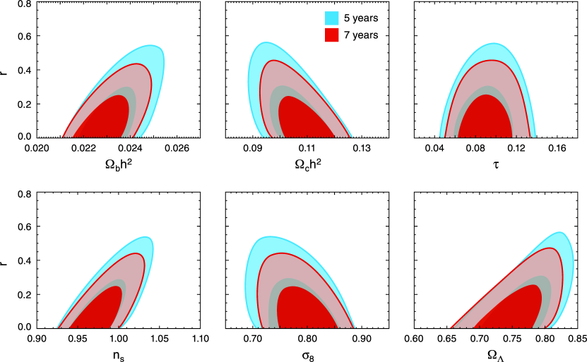
We do not detect gravitational waves from inflation with the 7-year WMAP data, however the upper limits are 16% lower: compared to . Figure 13 shows the the 2-d likelihood contours for vs. the other parameters using both the 5-year and 7-year WMAP data. This shows both the improved upper limit on and the correlations with the other measured parameters, especially the matter densities and . The limits quoted above arise from all of the power spectra measured by WMAP with the greatest power coming from the shape of the TT spectrum. Komatsu et al. (2010) consider the constraints that arise from polarization alone and show that the limits improve from to using the 5-year and 7-year data, respectively.
4.2.2 Scale Dependent Spectral Index
| Parameter | +Tensors | +Running | +Tensors+Running |
|---|---|---|---|
| Fit parameters | |||
| Derived parameters | |||
Some inflation models predict a scale dependence or “running” in the (nearly) power-law spectrum of scalar perturbations. This is conveniently parameterized by the logarithmic derivative of the spectral index, , which gives rise to a spectrum of the form (Kosowsky & Turner, 1995)
| (12) |
with Mpc-1. In the Markov chain, we use a flat prior on .
We do not detect a statistically significant (i.e., 95% CL) deviation from a pure power-law spectrum with the 7-year WMAP data. The allowed range of is both closer to zero and has a smaller confidence range using the 7-year data: compared to from the 5-year data.
If we allow both tensors and running as additional primordial degrees of freedom, the data prefer a slight negative running, but still at less than . The joint constraint on all parameters in this model is significantly tighter with the 7-year data (see §4.3). The 7-year constraints on models with additional power spectrum degrees of freedom are given in Table 4.
4.2.3 Isocurvature Modes
| Parameter | bbRepeated from Table 3 for comparison. | +anti-correlatedccAdds curvaton-type isocurvature perturbations (Komatsu et al., 2010). | +uncorrelatedddAdds axion-type isocurvature perturbations (Komatsu et al., 2010). |
|---|---|---|---|
| Fit parameters | |||
| Derived parameters | |||
In addition to adiabatic fluctuations, where different species fluctuate in phase to produce curvature fluctuations, it is possible to have an overdensity in one species compensate for an underdensity in another without producing a curvature. These entropy, or isocurvature perturbations have a measurable effect on the CMB by shifting the acoustic peaks in the power spectrum. For cold dark matter and photons, we define the field
| (13) |
(Bean et al., 2006; Komatsu et al., 2009). The relative amplitude of its power spectrum is parameterized by ,
| (14) |
with Mpc-1.
We consider two types of isocurvature modes: those which are completely uncorrelated with the curvature modes (with amplitude ), motivated with the axion model, and those which are anti-correlated with the the curvature modes (with amplitude ), motivated with the curvaton model. For the latter, we adopt the convention in which anticorrelation increases the power at low multipoles (Komatsu et al., 2009). For both and , we adopt a flat prior and require , .
The constraints on both types of isocurvature modes are given in Table 5. We do not detect a significant contribution from either type of perturbation in the 7-year data. The limit on uncorrelated modes improves the most with the new data: from to using the 5-year and 7-year data, respectively. Table 5 also shows that the standard parameters are only weakly affected by the isocurvature degrees of freedom. Komatsu et al. (2010) derive analogous constraints using a combination of WMAP plus other data. They find limits that are roughly a factor of two lower than the WMAP-only limits.
4.2.4 Spatial Curvature
| Parameter | bbRepeated from Table 3 for comparison. | OccAdds spatial curvature as a parameter, with . is imposed as a prior. | CDMddAdds dark energy equation of state as a parameter, with . is imposed as a prior. |
|---|---|---|---|
| Fit parameters | |||
| Derived parameters | |||
The basic model of the universe is flat, with . There is a compelling theoretical case for a flat universe in General Relativity, arising from the apparent paradox that a flat geometry is dynamically unstable. That is, in order for the curvature to be acceptably small today, say , the curvature in the early universe had to be extraordinarily fine tuned. Cosmological inflation achieves this by expanding the primordial curvature scale, if any, to super-horizon scales today.
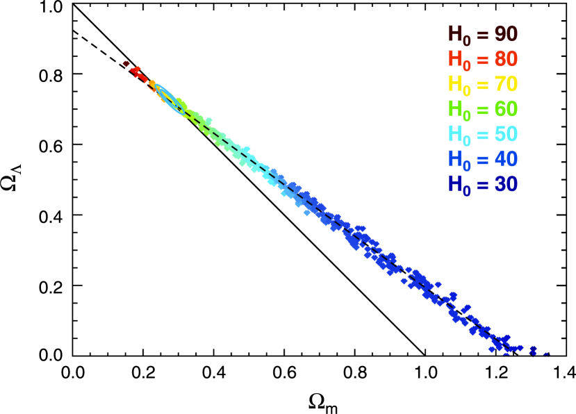
With knowledge of the redshift of matter-radiation equality, the acoustic scale can be accurately computed for use as a standard ruler at the epoch of recombination. The first acoustic peak in the CMB then provides a means to measure the angular diameter of the acoustic scale at the surface of last scattering. If we have independent knowledge of the local distance-redshift relation (the Hubble constant, ) we can infer the physical distance to the last scattering surface, and hence the geometry of the universe. If we assume nothing about we are left with a geometric degeneracy which is illustrated in Figure 14.
Assuming dynamics, WMAP data alone provide a remarkably simple constraint on the geometry and matter-energy content in the universe. The geometric degeneracy in the 7-year data is well described by (the dashed line in Figure 14). We have placed a flat prior on , and we now also constrain . The Figure also quantitatively illustrates how knowledge of the Hubble constant fixes the geometry, , and vice-versa. The points in the plot are culled from the Markov Chain that samples this model and their color is coded by the value of the Hubble constant for that sample. As one moves down the degeneracy line, the Hubble constant must decrease for the model to remain consistent with the geometry imposed by the CMB. For a flat universe the 7-year data give (Table 3), in excellent agreement with more traditional measurements of the Hubble constant, e.g, Riess et al. (2009).
If we allow curvature as a parameter, the 7-year WMAP data improve on the 5-year constraint by 11%, to . While this result is consistent with a flat universe, the preferred model is slightly closed and has a relatively low Hubble constant due to the geometric degeneracy, . Therefore, if we impose local distance scale measurements in the form of and BAO data, the limits on curvature tighten significantly to (Komatsu et al., 2010).
4.2.5 Non- Dark Energy
Dark energy is believed to be driving the present-day acceleration of the universe. Current measurements are consistent with the dark energy being a cosmological constant, or vacuum energy. If it is not a cosmological constant, then its physical density may change with the expansion of the universe. This, in turn, would affect the expansion history and the rate of large-scale structure growth in the universe. The evolution of its physical density is governed by its equation of state where is the pressure of the dark energy and its density. The cosmological constant has an equation of state . It would be tremendously important if observations could determine that since that would rule out the prime candidate for the dark energy and provide important new clues about physics.
Since the CMB primarily probes the high redshift universe (), and the effects of dark energy only start to dominate at relatively low redshift (), the CMB is not especially sensitive to subtle properties of the dark energy. Nonetheless, meaningful constraints on the equation of state can be inferred from the 7-year WMAP data. If we assume the universe is flat but let be a parameter in the Friedmann equation (with a flat prior on , , and ), we obtain the constraints given in Table 6. In particular, the 7-year data give , which is consistent with a cosmological constant. Komatsu et al. (2010) investigate the constraints imposed when 7-year WMAP data are combined with other observations. With BAO and Hubble constant measurements added, they find , which provides compelling limits on without using Type Ia supernovae data. When SNe data are included, the result becomes , but the quoted error does not include systematic errors in the supernovae, which are comparable to the statistical errors. Accounting for this would produce a final uncertainty that is roughly half the size of the error without SNe data.
If we relax the assumption that and/or , the constraints on weaken (Komatsu et al., 2010). This points to the need for more accurate and precise measurements of the expansion history and growth rate of structure if we are to gain further clues about dark energy from cosmology.
4.2.6 Neutrinos
| Parameter | bbRepeated from Table 3 for comparison. | +ccAllows effective number of relativistic species to vary (cf. =3.04). is imposed as a prior. | +ddAdds neutrino mass, , as a parameter, assuming =3.04 and degenerate mass eigenstates. |
|---|---|---|---|
| Fit parameters | |||
| Derived parameters | |||
Neutrinos affect the CMB spectrum in a variety of ways; one is by providing relativistic degrees of freedom to the plasma prior to recombination. Since neutrinos, or other relativistic species, are not coupled to the photon-baryon fluid, they free-stream out of over-densities and damp the acoustic oscillations prior to recombination. This action suppresses the peaks in the angular power spectrum somewhat; the amplitude of the effect depends on the effective number of relativistic degrees of freedom. Using the 7-year WMAP data we place a 95% CL lower limit of on the number of relativistic degrees of freedom, for a flat prior . (The standard model has .) This new limit is 17% higher than the 5-year limit of – due to the improved third peak measurement – and is now quite close to the standard model value.
The mean energy of a relativistic neutrino at the epoch of recombination is eV. In order for the CMB power spectrum to be sensitive to a non-zero neutrino mass, at least one species of neutrino must have a mass in excess of this mean energy (Komatsu et al., 2009). If one assumes that there are neutrino species with degenerate mass eigenstates, this would suggest that the lowest total mass that could be detected with CMB data is eV. Using a refined argument, Ichikawa et al. (2005) argue that one could reach 1.5 eV. When we add as a parameter to the model (and a flat prior on the physical neutrino density, , constrained by ), we obtain the fit given in Table 7, specifically , which is unchanged from the 5-year result and is slightly below the basic limits just presented. Note that these results come from the WMAP data alone. Tighter limits may be obtained by combining CMB data with measurements of structure formation, as discussed in Komatsu et al. (2010) and references therein.
4.2.7 Width of Reionization
| Parameter | bbRepeated from Table 3 for comparison. | +ccAllows width of reionization to vary. The constraints on are limited by the prior and so are not listed in the table. | +ddAllows primordial helium mass fraction to vary (cf. =0.24). |
|---|---|---|---|
| Fit parameters | |||
| Derived parameters | |||
Effective with the March 2008 version of the code CAMB (Lewis, 2008), a new parameter has been added which allows users to vary the reionization profile while holding the total optical depth fixed. The basic profile is a smooth ramp in redshift space and the parameter, , changes the slope of the ramp about its midpoint in such a way as to preserve total optical depth.
We have added as a parameter to the basic model, with a flat prior in the range , and present the results in Table 8.
4.2.8 Primordial Helium Abundance
Helium is thought to be synthesized in the early universe via Big Bang Nucleosynthesis (BBN). Given the WMAP measurement of the baryon-to-photon ratio, , the BBN-predicted yield for helium is =0.249 (Steigman, 2007). To date, the best technique for measuring the primordial abundance has been to observe stars in HII regions: in these systems, the helium abundance as a function of metallicity can be observed and the relation can be regressed to zero metallicity, which is presumed to give the primordial abundance (Gruenwald et al., 2002; Izotov & Thuan, 2004; Olive & Skillman, 2004; Fukugita & Kawasaki, 2006; Peimbert et al., 2007) as reviewed by Steigman (2007).
Primordial helium affects the time profile of recombination which, in turn, affects the CMB angular power spectrum, especially the third acoustic peak. With WMAP’s improved measurement of this peak, it is now possible to let be a fitted parameter in the model. We use a flat prior with . We present the results of this fit in Table 8 and call out the helium abundance specifically: . This result is consistent with the BBN prediction and suggests the existence of pre-stellar helium, at the level. Komatsu et al. (2010) consider the constraints that can be applied when higher-resolution CMB data are included in the fit. They find that the combined CMB data produce, for the first time, evidence for pre-stellar helium at .
4.3. Volume Change
| Model | Dimension | RatiobbThe ratio of allowable parameter-space volume: 5-year over 7-year, when fit to WMAP data only. |
|---|---|---|
| (Table 3) | 6 | 1.5 |
| +tensors (Table 4) | 7 | 1.9 |
| +running (Table 4) | 7 | 1.7 |
| +tensors+running (Table 4) | 8 | 3.0 |
| +anticorrelated isocurvature (Table 5) | 7 | 1.9 |
| +uncorrelated isocurvature (Table 5) | 7 | 1.9 |
| +massive neutrinos (Table 3) | 7 | 1.8 |
| o (Table 6) | 7 | 1.8 |
| CDM (Table 6) | 7 | 1.5 |
The tables presented in this section quote parameter uncertainties for marginalized 1-dimensional likelihood profiles. With the 7-year and 5-year results side by side, one could infer the improvement in precision for any given parameter in any given model fit, and we have called out examples in the text. But it is difficult to measure the overall improvement in the model fits from this presentation. A better measure is given by comparing the allowable volume in -dimensional parameter space for each of the models.
As a proxy for allowable volume, we compute the square root of the determinant of the parameter covariance matrix for each model, using data from the Markov chains. For example, with the 6-parameter model, we compute the covariance matrix directly from the chain samples. The allowable volume ratio is defined as the ratio of the square root of the 5-year determinant to the corresponding 7-year value. Models with more fit parameters have more rows and columns in their covariance matrix. While this proxy is only proportional to the volume if the parameter distributions are Gaussian, the error in this approximation will be similar for both the 5-year and 7-year data sets, so a comparison is still valid.
Table 9 gives the change in allowable parameter-space volume as a ratio of the 5-year to 7-year value. These results are based on fits to WMAP data only. Overall, the 6-parameter model is measured a factor of 1.5 more precisely with the 7-year data while the model with 2 additional parameters, tensors plus a running spectral index, is measured a factor of 3 times more precisely. Models with one additional parameter typically improve by factors of 1.8 to 1.9.
5. GOODNESS OF FIT
Given a best-fit model from the MCMC analysis, we can ask how well the model fits the data. Given that the likelihood function is non-Gaussian, answering the question is not as straightforward as testing the per degree of freedom of the best-fit model. Instead we resort to Monte Carlo simulations and compare the absolute likelihood obtained from fitting the flight data to an ensemble of simulated values.
For testing goodness of fit, we generate 500 realizations of the 7-year sky map data that include the CMB signal and instrument noise. These are the same realizations as were used for parameter recovery in §3, and are discussed in more detail in Appendix A.
For each realization of a 7-year data set, we constructed the likelihood function appropriate to those data. This required forming the high- MASTER spectra and the low-resolution sky maps used in the code. (For this study we did not employ Gibbs sampling for the low- TT likelihood, rather we used a direct pixel-space code that was computationally slower than the Blackwell-Rao estimate per likelihood evaluation, but it required less setup overhead per data realization.) For goodness of fit testing, we evaluated the likelihood of the input model for each data realization.
Due to its hybrid nature, the likelihood produces several components that need to be combined to obtain the full likelihood. The components of most interest to goodness of fit testing are the high- TT and TE portions, which cover the bulk of the multipole range and are the most straightforward to interpret. Recall the the high- TT component contains both a Gaussian and a log-normal contribution, as per equation 11 of Verde et al. (2003)
| (15) |
Here the first term can be compared to , as per equation 6 of Verde et al. (2003)
| (16) |
where is the inverse covariance matrix of the observed power spectrum , and is the model spectrum. The high- portion of the TE likelihood includes only the Gaussian component, which is a good approximation given the lower signal-to-noise ratio of the TE data. In the following, we report on the distribution of which we call the effective .
We compare the distribution of effective values for the high- TT portion of the likelihood, which contains 1170 multipoles from –1200, to a distribution with 1170 degrees of freedom. The agreement between the two distributions is good. We tentatively attribute a small shape difference between them to the non-Gaussian component in the likelihood. The effective for the 7-year flight TT spectrum is 1227 for 1170 degrees of freedom, after marginalizing over point sources and the SZ spectrum (which are not in the simulations). According to the Monte Carlo distribution, of the realizations had a higher effective , indicating that the flight data are reasonably well fit by the model spectrum.
We perform a similar comparison for the high- TE data, which covers the multipole range –800. One point of note is that we have adjusted our empirical calibration of as a result of these simulations: the new value is 1.011 times larger than we used in the 5-year analysis, which is equivalent to over-estimating the 5-year TE errors by 1.1%. The re-calibrated Monte Carlo distribution tracks the pure distribution, consistent with the high- TE likelihood being Gaussian. The effective for the 7-year flight TE spectrum is 807 for 777 degrees of freedom (again, after marginalization over point sources and the SZ spectrum). According to the Monte Carlo distribution, of the simulations had a higher effective , which could easily happen by random chance. This indicates that the theory yields a TE spectrum that fits the data well.
6. CONCLUSIONS
We present the angular power spectra derived from the 7-year WMAP sky maps and discuss the cosmological conclusions that can be inferred from WMAP data alone.
With the 7-year data, the temperature (TT) spectrum measurement is now limited by cosmic variance for multipoles , and the signal-to-noise ratio per multipole exceeds unity for . In a band-power of width the signal-to-noise ratio exceeds unity to . The third acoustic peak in the TT spectrum is now well measured by WMAP. In the context of a flat model, this improvement allows us to place tighter constraints on the matter density from WMAP data alone, , and on the epoch of matter-radiation equality, . The temperature-polarization (TE) spectrum is detected in the 7-year data with a significance of , compared to with the 5-year data. We now detect the second dip in the TE spectrum near with high confidence. The TB and EB spectra remain consistent with zero in the 7-year data. This demonstrates low systematic errors in the data and is used to place 33% tighter limits on the rotation of linear polarization due to parity-violating effects: (Komatsu et al., 2010). The low- EE spectrum, a measure of the optical depth due to reionization, is detected at significance when averaged over –7: K2 (68% CL). The high- EE spectrum in the range is detected at over 8 . The BB spectrum, an important probe of gravitational waves from inflation, remains consistent with zero; when averaged over –7, K2 (95% CL). The upper limit on tensor modes from polarization data alone is a factor of 2 lower with the 7-year data than it was using the 5-year data (Komatsu et al., 2010).
The data remain consistent with the simple model. The best-fit parameter values are given in Table 3; the TT spectrum from this fit has an effective of 1227 for 1170 degrees of freedom, with a probability to exceed of 9.6%. The allowable volume in the 6-dimensional space of parameters has been reduced by a factor of 1.5 relative to the 5-year volume. Most models with one additional parameter beyond see volume reduction factors of 1.8–1.9, while the model that allows for tensor modes and a running scalar spectral index has a factor of 3 lower volume when fit to the 7-year data. We test the parameter recovery process for bias and find that the scalar spectral index, , is biased high, but only by , while the remaining parameters are biased by .
The improvement in the third peak measurement leads to tighter lower limits from WMAP on the number of relativistic degrees of freedom (e.g., neutrinos) in the early universe: . Also, using WMAP data alone, the primordial helium mass fraction is found to be , and with data from higher-resolution CMB experiments included, Komatsu et al. (2010) establish the existence of pre-stellar helium at .
Appendix A PARAMETER RECOVERY SIMULATIONS
This appendix describes the configuration of the set of 500 simulations that was used for checking parameter recovery and the values from the likelihood.
The mask is the KQ85y7 mask, which lets through 78.3% of the sky.
For instrument noise, we employ a 2-step process in which we generate uncorrelated noise at high resolution and combine it with low resolution correlated noise. The noise was constructed from the 7-year and 1024 maps, the 7-year covariance matrices, the 7-year values, and the 7-year synchrotron cleaning factors, given in Gold et al. (2010). For each year and nine DAs (Ka1–W4), a high resolution uncorrelated noise map was made with I, Q, U components at and and 1024, including the QU correlations within each pixel. The noise maps are generated on a single-year, single-DA basis so we can mimic the construction of the flight spectra and likelihood function. A correlated noise map was made at . The values for the polarization portion of these maps were increased by a factor of , where is the fraction of the K band map which has been removed to avoid synchrotron contamination (Gold et al., 2010). This accounts for the increased noise due to the synchrotron template subtraction. We combined the low resolution () and high resolution ( or 1024) maps by subtracting off the mean of the high resolution noise within each low resolution pixel, and then added the low resolution noise to all high resolution pixels within that low resolution pixel. This process provides a high resolution noise realization that has the proper low resolution noise correlations when it is binned. Note that the and 1024 maps have different noise realizations, but this will have no effect on the resultant likelihoods, because the maps are used for polarization and the maps are used for temperature, following the procedure used in the standard WMAP pipeline.
The CMB signal is assumed to be Gaussian, and random-phase, and so its statistical properties are completely defined by a power spectrum. The parameter recovery simulations all use the same power spectrum, which was derived from the best fit to a 5-year Markov chain, with WMAP, Baryon Acoustic Oscillation, and Supernova data. The parameters used are , , , , , . The gravitational lensing signal is treated as Gaussian, and the effects on the temperature and polarization power spectra are included. However, the BB spectrum has been zeroed, for consistency with a map-making simulation done previously. Zeroing the BB spectrum will have no effect on parameter recovery, since our simple model has a tensor to scalar ratio of 0, and therefore an undetectable BB spectrum. Each CMB realization has the same theoretical power spectrum, but different cosmic variance. The different DAs in a given realization all see the same CMB sky, but with different smoothing, and different noise. The smoothing used for each DA is a circular beam response based on the appropriate 7-year beam transfer function (Jarosik et al., 2010).
These simulations do not include foregrounds, the Sunyaev-Zel’dovich effect, unresolved point sources, or beam uncertainty.
The analysis of the parameter recovery simulations uses the same parameters as went into the maps, in the case of , beam profiles, and usage of gravitational lensing. However, for the and synchrotron cleaning coefficients, the simulations were produced with the 7-year values, and analyzed with the previous 5-year values. Note that this is a small difference, because the 7-year values are not very different from the 5-year values.
The parameter recovery importance sampling used the September 2008 version of CAMB, and so does not include the bug fix for the proton mass error. This has no effect on the simple model explored here.
Appendix B RECFAST AND WMAP LIKELIHOOD UPDATES
| Parameter | UpdatedbbThe updated version of the parameters, based on RECFAST 1.5 and version 4.1 of the WMAP likelihood. This version is more accurate, but was not available when the chains in the rest of this paper were run. | OriginalccThe original version of the parameters, based on RECFAST 1.4.2 and version 4.0 of the WMAP likelihood. This is the code configuration used for the chains reported in this paper. |
|---|---|---|
| Fit parameters | ||
| Derived parameters | ||
As mentioned in §2.6, since the original version of this paper, there have been two updates to the parameter estimation code: an improvement in RECFAST from version 1.4.2 to version 1.5, which includes an improved model of the hydrogen atom; and a small bug fix in the WMAP likelihood code, changing its version from 4.0 to 4.1.
We have rerun the parameter fits using the version 4.1 likelihood, and find parameter changes of order 0.1 . The effect on parameters of updating to the new version of RECFAST in CAMB is also of order 0.1 . The largest combined changes are an increase in of 0.35 , and an increase in the spectral index of 0.26 ; Table 10 provides more detailed information on several original and updated parameter values.
References
- Bean et al. (2006) Bean, R., Dunkley, J., & Pierpaoli, E. 2006, Phys. Rev., D74, 063503
- Bennett et al. (2003a) Bennett, C. L., et al. 2003a, ApJS, 148, 1
- Bennett et al. (2003b) —. 2003b, ApJ, 583, 1
- Bennett et al. (2010) Bennett, C. L. et al. 2010, Astrophys. J. Suppl., submitted
- Bond et al. (1998) Bond, J. R., Jaffe, A. H., & Knox, L. 1998, Phys. Rev. D, 57, 2117
- Brown et al. (2009) Brown, M. L., et al. 2009, ApJ, 705, 978
- Chu et al. (2005) Chu, M., Eriksen, H. K., Knox, L., Górski, K. M., Jewell, J. B., Larson, D. L., O’Dwyer, I. J., & Wandelt, B. D. 2005, Phys. Rev. D, 71, 103002
- Colombo & Pierpaoli (2010) Colombo, L. P. L. & Pierpaoli, E. 2010, ArXiv e-prints
- Dunkley et al. (2009) Dunkley, J., et al. 2009, ApJS, 180, 306
- Eriksen et al. (2004) Eriksen, H. K., et al. 2004, ApJS, 155, 227
- Eriksen et al. (2007) —. 2007, ApJ, 656, 641
- Fukugita & Kawasaki (2006) Fukugita, M. & Kawasaki, M. 2006, ApJ, 646, 691
- Gold et al. (2009) Gold, B., et al. 2009, ApJS, 180, 265
- Gold et al. (2010) Gold, B. et al. 2010, Astrophys. J. Suppl., submitted
- Goldberg et al. (1967) Goldberg, J. N., MacFarlane, A. J., Newman, E. T., Rohrlich, F., & Sudarshan, E. C. G. 1967, J. Math. Phys., 8, 2155
- Gorski et al. (2005) Gorski, K. M., Hivon, E., Banday, A. J., Wandelt, B. D., Hansen, F. K., Reinecke, M., & Bartlemann, M. 2005, ApJ, 622, 759
- Gruenwald et al. (2002) Gruenwald, R., Steigman, G., & Viegas, S. M. 2002, ApJ, 567, 931
- Gruppuso et al. (2009) Gruppuso, A., de Rosa, A., Cabella, P., Paci, F., Finelli, F., Natoli, P., de Gasperis, G., & Mandolesi, N. 2009, MNRAS, 400, 463
- Hinshaw et al. (2003) Hinshaw, G., et al. 2003, ApJS, 148, 135
- Hinshaw et al. (2007) —. 2007, ApJS, 170, 288
- Hivon et al. (2002) Hivon, E., Górski, K. M., Netterfield, C. B., Crill, B. P., Prunet, S., & Hansen, F. 2002, ApJ, 567, 2
- Ichikawa et al. (2005) Ichikawa, K., Fukugita, M., & Kawasaki, M. 2005, Phys. Rev. D, 71, 043001
- Izotov & Thuan (2004) Izotov, Y. I. & Thuan, T. X. 2004, ApJ, 602, 200
- Jarosik et al. (2010) Jarosik, N. et al. 2010, Astrophys. J. Suppl., submitted
- Jewell et al. (2004) Jewell, J., Levin, S., & Anderson, C. H. 2004, ApJ, 609, 1
- Jewell et al. (2009) Jewell, J. B., Eriksen, H. K., Wandelt, B. D., O’Dwyer, I. J., Huey, G., & Górski, K. M. 2009, ApJ, 697, 258
- Kamionkowski et al. (1997) Kamionkowski, M., Kosowsky, A., & Stebbins, A. 1997, Phys. Rev. D, 55, 7368
- Komatsu & Seljak (2002) Komatsu, E. & Seljak, U. 2002, MNRAS, 336, 1256
- Komatsu et al. (2003) Komatsu, E., et al. 2003, ApJS, 148, 119
- Komatsu et al. (2009) —. 2009, ApJS, 180, 330
- Komatsu et al. (2010) Komatsu, E. et al. 2010, Astrophys. J. Suppl., submitted, arXiv:1001.4538
- Kosowsky & Turner (1995) Kosowsky, A. & Turner, M. S. 1995, Phys. Rev. D, 52, 1739
- Larson (2006) Larson, D. L. 2006, Ph.D. thesis, University of Illinois at Urbana-Champaign
- Lewis (2008) Lewis, A. 2008, Phys. Rev., D78, 023002
- Lewis et al. (2000) Lewis, A., Challinor, A., & Lasenby, A. 2000, ApJ, 538, 473
- Mackay (2003) Mackay, D. 2003, Information Theory, Inference, and Learning Algorithms (Cambridge University Press)
- Newman & Penrose (1966) Newman, E. T. & Penrose, R. 1966, Journal of Mathematical Physics, 7, 863
- Nolta et al. (2009) Nolta, M. R., et al. 2009, ApJS, 180, 296
- O’Dwyer et al. (2004) O’Dwyer, I. J. et al. 2004, Astrophys. J., 617, L99
- Olive & Skillman (2004) Olive, K. A. & Skillman, E. D. 2004, ApJ, 617, 29
- Page et al. (2007) Page, L., et al. 2007, ApJS, 170, 335
- Peimbert et al. (2007) Peimbert, M., Luridiana, V., & Peimbert, A. 2007, ApJ, 666, 636
- Riess et al. (2009) Riess, A. G., et al. 2009, ApJ, 699, 539
- Rudjord et al. (2009) Rudjord, Ø., Groeneboom, N. E., Eriksen, H. K., Huey, G., Górski, K. M., & Jewell, J. B. 2009, ApJ, 692, 1669
- Scott & Moss (2009) Scott, D. & Moss, A. 2009, MNRAS, 397, 445
- Seager et al. (1999) Seager, S., Sasselov, D. D., & Scott, D. 1999, ApJ, 523, L1
- Seager et al. (2000) —. 2000, ApJS, 128, 407
- Seljak & Zaldarriaga (1996) Seljak, U. & Zaldarriaga, M. 1996, ApJ, 469, 437
- Spergel et al. (2003) Spergel, D. N., et al. 2003, ApJS, 148, 175
- Spergel et al. (2007) —. 2007, ApJS, 170, 377
- Steigman (2007) Steigman, G. 2007, Annual Review of Nuclear and Particle Science, 57, 463
- Verde et al. (2003) Verde, L., et al. 2003, ApJS, 148, 195
- Verde et al. (2003) Verde, L. et al. 2003, Astrophys. J. Suppl., 148, 195
- Wandelt et al. (2004) Wandelt, B. D., Larson, D. L., & Lakshminarayanan, A. 2004, Phys. Rev. D, 70, 083511
- Weiland et al. (2010) Weiland, J. L. et al. 2010, Astrophys. J. Suppl., submitted
- Wong et al. (2008) Wong, W. Y., Moss, A., & Scott, D. 2008, MNRAS, 386, 1023
- Zaldarriaga & Seljak (1997) Zaldarriaga, M. & Seljak, U. 1997, Phys. Rev. D, 55, 1830