TTP 10-04 January 19, 2010

Higgs Pseudo-Observables,
Second Riemann Sheet and All That 999This work is supported by the European Community’s Marie Curie Research Training Network Tools and Precision Calculations for Physics Discoveries at Colliders under contract MRTN-CT-2006-035505, by the U.S. Department of Energy under contract No. DE-AC02-98CH10886 and by the Deutsche Forschungsgemeinschaft through Sonderforschungsbereich/Transregio 9 Computergestützte Theoretische Teilchenphysik.

Giampiero Passarino ***giampiero@to.infn.it

Dipartimento di Fisica Teorica, Università di Torino, Italy
INFN, Sezione di Torino, Italy

Christian Sturm sturm@bnl.gov

Physics Department, Brookhaven National Laboratory,
Upton, NY 11973, USA

Sandro Uccirati uccirati@particle.uni-karlsruhe.de

Institut für Theoretische Teilchenphysik, Universität Karlsruhe,
76128 Karlsruhe, Germany

The relation between physical observables measured at LHC and Tevatron and standard model Higgs pseudo-observables (production cross section and partial decay widths) is revised by extensively using the notion of the Higgs complex pole on the second Riemann sheet of the S𝑆S\,-matrix. The extension of their definition to higher orders is considered, confronting the problems that arise when QED(QCD) corrections are included in computing realistic observables. Numerical results are presented for pseudo-observables related to the standard model Higgs boson decay and production. The relevance of the result for exclusion plots of the standard model Higgs boson for high masses (up to 600600600\,GeV) is discussed. Furthermore, a recipe for the analytical continuation of Feynman loop integrals from real to complex internal masses and complex Mandelstam invariants is thoroughly discussed.

Keywords: Feynman diagrams, Loop calculations, Radiative corrections, Higgs physics

PACS classification: 11.15.Bt, 12.38.Bx, 13.85.Lg, 14.80.Bn, 14.80.Cp

1 Introduction

The search for a mechanism explaining electroweak symmetry breaking has been a major goal for many years, in particular the search for a standard model (SM) Higgs boson, see for instance Ref. [1] and Ref. [2]. As a result of this an intense effort in the theoretical community has been made to produce the most accurate NLO and NNLO predictions, see Refs. [3, 4, 5, 6]. There is, however, a point that has been ignored in all these calculations: the Higgs boson is an unstable particle and should be removed from the in/out bases in the Hilbert space, without destroying the unitarity of the theory. Therefore, concepts as the production of an unstable particle or its partial decay widths do not have a precise meaning and should be replaced by a conventionalized definition which respects first principles of quantum field theory (QFT).

The quest for a proper treatment of a QFT of unstable particles dates back to the sixties and to the work of Veltman [8] (for earlier attempts see Ref. [9]); more recently the question has been readdressed by Sirlin and collaborators [10]. Alternative approaches, within the framework of an effective theory can be found in Ref. [11].

In this paper we discuss the relation between physical observables and Higgs pseudo-observables by considering the extension of their definition to higher orders in perturbation theory, confronting the problems that arise when perturbative corrections in quantum electrodynamics (QED) and quantum chromodynamics (QCD) are included. Numerical results are also presented. Our work can be seen as an extension of complex-mass schemes to include complex external momenta (for previous work see also Ref. [12]), addressing systematically the question of the analytical continuation of Feynman loop integrals.

This paper is organized as follows. In Section 2 we summarize the conceptual setup. In Section 3 we present general arguments on complex poles. In Section 4 and 5 we discuss pseudo-observables, on-shell observables and unitarity. The analytical continuation of Feynman loop integrals into the second Riemann sheet of the S𝑆S\,-matrix is examined in Section 6. In Section 7 we present the inclusion of QED and QCD corrections and renormalization schemes are highlighted in Section 8. Numerical results are given in Section 9 and in Section 10 we close with our conclusions.

2 Formulation of the problem

There are two old questions in relating measurements to theoretical predictions:

  • Experimenters (should) extract so-called realistic observables from raw data, e.g. σ(ppγγ+X)𝜎𝑝𝑝𝛾𝛾𝑋\sigma(pp\to\gamma\gamma+X) and need to present results in a form that can be useful for comparing them with theoretical predictions, i.e. the results should be transformed into pseudo-observables; during the deconvolution procedure one should also account for the interference background – signal;

  • Theorists (should) compute pseudo-observables using the best available technology and satisfying a list of demands from the self-consistency of the underlying theory [14].

Almost from the start it is clear that a common language must be established in order to avoid misunderstandings and confusion. A typical example can be found in Higgs physics where, frequently, one talks about Higgs production cross section or Higgs partial decay widths. After the discovery phase, in absence of which the future of high energy physics cannot be ascertained, one will need to probe the properties of the discovered resonance, like spin and couplings. In this case different sources will start talking about the same thing but with different languages. We will indicate a reasonable language within the context of a perturbative expansion of a gauge-invariant QFT in this paper.

The Higgs boson, as well as the W𝑊W or Z𝑍Z bosons, are unstable particles; as such they should be removed from in/out bases in the Hilbert space, without changing the unitarity of the theory. As mentioned before, concepts as the production of an unstable particle or its partial decay widths, not having a precise meaning, are only an approximation of a more complete description. The inconsistencies associated with the on-shell LSZ formulation of an unstable external particles become particularly severe starting from two-loops, as described in Ref. [5].

Suppose that we want to combine a Higgs production mechanism, say gluon-gluon fusion, with the subsequent decay Hγγ𝐻𝛾𝛾H\to\gamma\gamma. The process to be considered is, therefore, ppγγ+X𝑝𝑝𝛾𝛾𝑋pp\to\gamma\gamma+X and it is made of a part that defines the signal, e.g.

ppgg(Hγγ)+X,pp\to gg(\to H\to\gamma\gamma)+X, (1)

and by a non-resonant background. The question is: how to extract from the data, without ambiguities, a pseudo-observable to be termed Higgs partial decay width into two photons which, at the same time, does not violate first principles? Once again, one should be aware that there is no Higgs boson in the in-state, therefore the matrix element <γγout|Hin>inner-product𝛾𝛾out𝐻in<\gamma\gamma\;{\rm out}|H\;{\rm in}> is not definable in QFT and this ill-defined quantity should be replaced by a pseudo-observable which closely resembles the intuitive concept of a decay width, can be unambiguously extracted from the data and respects all fundamental properties of the theory; in this way we replace a non existing observable with a conventional definition. A proposal in this direction can be found in Ref.[10]; here we revise the proposal, improving it by considering the extension to higher orders in perturbation theory, confronting the problems that arise when QED(QCD) corrections have to be included and present numerical results for Higgs physics.

At the parton level the S𝑆S\,-matrix for the process if𝑖𝑓i\to f can be written as

Sfi=Vi(s)ΔH(s)Vf(s)+Bif(s),subscript𝑆𝑓𝑖subscript𝑉𝑖𝑠subscriptΔ𝐻𝑠subscript𝑉𝑓𝑠subscript𝐵𝑖𝑓𝑠S_{fi}=V_{i}(s)\,\Delta_{{\scriptscriptstyle{H}}}(s)\,V_{f}(s)+B_{if}(s), (2)

where Visubscript𝑉𝑖V_{i} is the production vertex iH𝑖𝐻i\to H (e.g. ggH𝑔𝑔𝐻gg\to H), Vfsubscript𝑉𝑓V_{f} is the decay vertex Hf𝐻𝑓H\to f (e.g. Hγγ𝐻𝛾𝛾H\to\gamma\gamma), ΔHsubscriptΔ𝐻\Delta_{{\scriptscriptstyle{H}}} is the Dyson re-summed Higgs propagator and Bifsubscript𝐵𝑖𝑓B_{if} is the non-resonant background (e.g. ggγγ𝑔𝑔𝛾𝛾gg\to\gamma\gamma boxes). In the next section we will introduce the notion of complex pole. A vertex is defined by the following decomposition [16],

Vf(s)=aVfa(s,{S})Ffa({pf})subscript𝑉𝑓𝑠subscript𝑎subscriptsuperscript𝑉𝑎𝑓𝑠𝑆subscriptsuperscript𝐹𝑎𝑓subscript𝑝𝑓V_{f}(s)=\sum_{a}\,V^{a}_{f}\left(s\,,\,\{S\}\right)\,F^{a}_{f}\left(\{p_{f}\}\right) (3)

where s=PH2𝑠superscriptsubscript𝑃𝐻2s=-P_{{\scriptscriptstyle{H}}}^{2} (with PH=fpfsubscript𝑃𝐻subscript𝑓subscript𝑝𝑓P_{{\scriptscriptstyle{H}}}=\sum_{f}p_{f}), s{S}direct-sum𝑠𝑆s\,\oplus\,\{S\} is the set of Mandelstam invariants that characterize the process Hf𝐻𝑓H\to f, Vfasubscriptsuperscript𝑉𝑎𝑓V^{a}_{f} are scalar form factors and the Ffasubscriptsuperscript𝐹𝑎𝑓F^{a}_{f} contain spinors, polarization vectors, etc.

3 The complex pole

In this section we introduce the notion of the complex pole [15] following closely the analysis of Ref. [17]. Let ΔisubscriptΔ𝑖\Delta_{i} be the lowest order propagator for particle i𝑖i and Δ¯isubscript¯Δ𝑖{\overline{\Delta}}_{i} the corresponding dressed propagator, i.e.

Δ¯i=Δi1+ΔiΣii,subscript¯Δ𝑖subscriptΔ𝑖1subscriptΔ𝑖subscriptΣ𝑖𝑖{\overline{\Delta}}_{i}=-\,\frac{\Delta_{i}}{1+\Delta_{i}\,\Sigma_{ii}}, (4)

Let us analyze in more details the definition of the dressed propagator: to begin with, consider a skeleton expansion of the self-energy S=16π4iΣ𝑆16superscript𝜋4𝑖ΣS=16\,\pi^{4}\,i\,\Sigma with propagators that are resummed up to 𝒪(n)𝒪𝑛{\cal O}\left(n\right) and define

Δi(n)(s)=Δi(0)(s)[1+Δi(0)(s)Σii(n)(s,Δi(n1)(s))]1,subscriptsuperscriptΔ𝑛𝑖𝑠subscriptsuperscriptΔ0𝑖𝑠superscriptdelimited-[]1subscriptsuperscriptΔ0𝑖𝑠subscriptsuperscriptΣ𝑛𝑖𝑖𝑠subscriptsuperscriptΔ𝑛1𝑖𝑠1\Delta^{(n)}_{i}(s)=-\,\Delta^{(0)}_{i}(s)\,\Bigl{[}1+\Delta^{(0)}_{i}(s)\,\Sigma^{(n)}_{ii}\left(s\,,\,\Delta^{(n-1)}_{i}(s)\right)\Bigr{]}^{-1}, (5)

where, omitting an overall factor i/(2π)4𝑖superscript2𝜋4-i/(2\,\pi)^{4}, the Born propagator (tensor structures are easily included) is

Δi(0)(s)=1smi2.subscriptsuperscriptΔ0𝑖𝑠1𝑠subscriptsuperscript𝑚2𝑖\Delta^{(0)}_{i}(s)=\frac{1}{s-m^{2}_{i}}. (6)

If it exists, we define a dressed propagator as the formal limit [8]

Δ¯i(s)=limnΔi(n)(s),Δ¯i(s)=Δi(0)(s)[1+Δi(0)(s)Σii(s,Δ¯i(s))]1,formulae-sequencesubscript¯Δ𝑖𝑠subscript𝑛subscriptsuperscriptΔ𝑛𝑖𝑠subscript¯Δ𝑖𝑠subscriptsuperscriptΔ0𝑖𝑠superscriptdelimited-[]1subscriptsuperscriptΔ0𝑖𝑠subscriptΣ𝑖𝑖𝑠subscript¯Δ𝑖𝑠1{\overline{\Delta}}_{i}(s)=\lim_{n\to\infty}\,\Delta^{(n)}_{i}(s),\qquad{\overline{\Delta}}_{i}(s)=-\,\Delta^{(0)}_{i}(s)\,\Bigl{[}1+\Delta^{(0)}_{i}(s)\,\Sigma_{ii}\left(s\,,\,{\overline{\Delta}}_{i}(s)\right)\Bigr{]}^{-1}, (7)

which coincides with the Schwinger-Dyson solution for the propagator.

The Higgs boson complex pole (sHsubscript𝑠𝐻s_{{\scriptscriptstyle{H}}}) is the solution of the equation

sHMH2+ΣHH(sH)=0,subscript𝑠𝐻subscriptsuperscript𝑀2𝐻subscriptΣ𝐻𝐻subscript𝑠𝐻0s_{{\scriptscriptstyle{H}}}-M^{2}_{{\scriptscriptstyle{H}}}+\Sigma_{{\scriptscriptstyle{H}\scriptscriptstyle{H}}}(s_{{\scriptscriptstyle{H}}})=0, (8)

where MH2subscriptsuperscript𝑀2𝐻M^{2}_{{\scriptscriptstyle{H}}} is the renormalized Higgs boson mass; here we assume that all counter-terms have been introduced to make the off-shell Green’s function ultraviolet finite, respecting locality of the counter-terms. We now examine more carefully the self-energy to all orders in perturbation theory since, often, there is some confusion with statements that are formulated to all orders and applied to a truncated perturbative expansion. Now consider the, all orders, self-energy,

ΣHH(s,MH2,ξ)=n=1ΣHH(n)(s,MH2,ξ)g2n,subscriptΣ𝐻𝐻𝑠subscriptsuperscript𝑀2𝐻𝜉superscriptsubscript𝑛1subscriptsuperscriptΣ𝑛𝐻𝐻𝑠subscriptsuperscript𝑀2𝐻𝜉superscript𝑔2𝑛\Sigma_{{\scriptscriptstyle{H}\scriptscriptstyle{H}}}(s,M^{2}_{{\scriptscriptstyle{H}}},\xi)=\sum_{n=1}^{\infty}\,\Sigma^{(n)}_{{\scriptscriptstyle{H}\scriptscriptstyle{H}}}(s,M^{2}_{{\scriptscriptstyle{H}}},\xi)\,g^{2n}, (9)

where ξ𝜉\xi is the gauge parameter (extension to more than one gauge parameters is straightforward) and g𝑔g is the renormalized coupling constant. From arguments based on Nielsen identities, see Ref [16], we know that

ξsH=0,ξΣHH(sH,MH2,ξ)=0,formulae-sequence𝜉subscript𝑠𝐻0𝜉subscriptΣ𝐻𝐻subscript𝑠𝐻subscriptsuperscript𝑀2𝐻𝜉0\frac{\partial}{\partial\xi}\,s_{{\scriptscriptstyle{H}}}=0,\qquad\frac{\partial}{\partial\xi}\,\Sigma_{{\scriptscriptstyle{H}\scriptscriptstyle{H}}}(s_{{\scriptscriptstyle{H}}},M^{2}_{{\scriptscriptstyle{H}}},\xi)=0, (10)

i.e. the location of the complex pole is ξ𝜉\xi independent; as a consequence the self-energy is ξ𝜉\xi independent too, since the two differ by a renormalized quantity, obviously ξ𝜉\xi independent. We consider first the one-loop approximation for the self-energy: from its explicit expression we are able to derive the following relation:

ΣHH(1)(s,MH2,ξ)=ΣHH;I(1)(s,MH2)+(sMH2)ΦH(s,MH2,ξ).subscriptsuperscriptΣ1𝐻𝐻𝑠subscriptsuperscript𝑀2𝐻𝜉subscriptsuperscriptΣ1𝐻𝐻𝐼𝑠subscriptsuperscript𝑀2𝐻𝑠subscriptsuperscript𝑀2𝐻subscriptΦ𝐻𝑠subscriptsuperscript𝑀2𝐻𝜉\Sigma^{(1)}_{{\scriptscriptstyle{H}\scriptscriptstyle{H}}}(s,M^{2}_{{\scriptscriptstyle{H}}},\xi)=\Sigma^{(1)}_{{\scriptscriptstyle{H}\scriptscriptstyle{H}}\,;\,{\scriptscriptstyle{I}}}(s,M^{2}_{{\scriptscriptstyle{H}}})+(s-M^{2}_{{\scriptscriptstyle{H}}})\,\Phi_{{\scriptscriptstyle{H}}}(s,M^{2}_{{\scriptscriptstyle{H}}},\xi). (11)

where, in a general Rξsubscript𝑅𝜉R_{\xi} gauge, we obtain

MW2ΦH=18{(s+MH2)[Bd(s,MZ2,MZ2;ξZ)+2Bd(s,MW,MW;ξW)]+2Ad(MZ,ξZ)+4Ad(MW,ξW)},subscriptsuperscript𝑀2𝑊subscriptΦ𝐻18𝑠subscriptsuperscript𝑀2𝐻delimited-[]subscript𝐵𝑑𝑠subscriptsuperscript𝑀2𝑍subscriptsuperscript𝑀2𝑍subscript𝜉𝑍2subscript𝐵𝑑𝑠subscript𝑀𝑊subscript𝑀𝑊subscript𝜉𝑊2subscript𝐴𝑑subscript𝑀𝑍subscript𝜉𝑍4subscript𝐴𝑑subscript𝑀𝑊subscript𝜉𝑊M^{2}_{{}_{W}}\Phi_{{\scriptscriptstyle{H}}}=-\frac{1}{8}\bigg{\{}(s\!+\!M^{2}_{{\scriptscriptstyle{H}}})\Bigl{[}B_{d}(s,M^{2}_{{}_{Z}},M^{2}_{{}_{Z}};\xi_{{\scriptscriptstyle{Z}}})+2\,B_{d}(s,M_{{}_{W}},M_{{}_{W}};\xi_{{\scriptscriptstyle{W}}})\Bigr{]}+2\,A_{d}(M_{{}_{Z}},\xi_{{\scriptscriptstyle{Z}}})+4\,A_{d}(M_{{}_{W}},\xi_{{\scriptscriptstyle{W}}})\bigg{\}},
Bd(s,m,m,ξ)=B0(s,ξm,ξm)B0(s,m,m),Ad(m,ξ)=A0(ξm)A0(m).formulae-sequencesubscript𝐵𝑑𝑠𝑚𝑚𝜉subscript𝐵0𝑠𝜉𝑚𝜉𝑚subscript𝐵0𝑠𝑚𝑚subscript𝐴𝑑𝑚𝜉subscript𝐴0𝜉𝑚subscript𝐴0𝑚B_{d}\left(s,m,m,\xi\right)=B_{0}\left(s,\xi\,m,\xi\,m\right)-B_{0}\left(s,m,m\right),\quad A_{d}\left(m,\xi\right)=A_{0}(\xi\,m)-A_{0}(m). (12)

The symbols A0,B0,subscript𝐴0subscript𝐵0A_{0},B_{0},\, etc. are the usual scalar, one-loop functions.

It needs to be stressed that the splitting between gauge dependent and gauge independent quantities is only defined modulo a ξ𝜉\xi\,-independent constant. Our definition of the invariant part is that it coincides with the expression in the ’t Hooft-Feynman gauge (i.e. ξ=1𝜉1\xi=1). Furthermore, finite renormalization (i.e. replacing renormalized parameters with a set of experimental data points after having removed ultraviolet poles by means of local counter-terms) amounts to replace

MH2=sH+ΣHH(sH,MH2,ξ),subscriptsuperscript𝑀2𝐻subscript𝑠𝐻subscriptΣ𝐻𝐻subscript𝑠𝐻subscriptsuperscript𝑀2𝐻𝜉M^{2}_{{\scriptscriptstyle{H}}}=s_{{\scriptscriptstyle{H}}}+\Sigma_{{\scriptscriptstyle{H}\scriptscriptstyle{H}}}(s_{{\scriptscriptstyle{H}}},M^{2}_{{\scriptscriptstyle{H}}},\xi), (13)

showing that

ξΣHH(1)(sH,sH,ξ)=0,𝜉subscriptsuperscriptΣ1𝐻𝐻subscript𝑠𝐻subscript𝑠𝐻𝜉0\frac{\partial}{\partial\xi}\,\Sigma^{(1)}_{{\scriptscriptstyle{H}\scriptscriptstyle{H}}}(s_{{\scriptscriptstyle{H}}},s_{{\scriptscriptstyle{H}}},\xi)=0, (14)

so that, at one-loop, the Higgs complex pole is gauge parameter independent if the self-energy is computed at MH2=sHsubscriptsuperscript𝑀2𝐻subscript𝑠𝐻M^{2}_{{\scriptscriptstyle{H}}}=s_{{\scriptscriptstyle{H}}}, the basis of the so-called complex-mass scheme (see Ref. [18] and also Ref. [17]). From Eq.(10) and from the one-loop result in Eq.(11), we derive the following

ΣHH(n)(sH,MH2,ξ)subscriptsuperscriptΣ𝑛𝐻𝐻subscript𝑠𝐻subscriptsuperscript𝑀2𝐻𝜉\displaystyle\Sigma^{(n)}_{{\scriptscriptstyle{H}\scriptscriptstyle{H}}}(s_{{\scriptscriptstyle{H}}},M^{2}_{{\scriptscriptstyle{H}}},\xi) =\displaystyle= ΣHH;I(n)(sH,MH2)+ΣHH;ξ(n)(sH,MH2,ξ),subscriptsuperscriptΣ𝑛𝐻𝐻𝐼subscript𝑠𝐻subscriptsuperscript𝑀2𝐻subscriptsuperscriptΣ𝑛𝐻𝐻𝜉subscript𝑠𝐻subscriptsuperscript𝑀2𝐻𝜉\displaystyle\Sigma^{(n)}_{{\scriptscriptstyle{H}\scriptscriptstyle{H}}\,;\,{\scriptscriptstyle{I}}}(s_{{\scriptscriptstyle{H}}},M^{2}_{{\scriptscriptstyle{H}}})+\Sigma^{(n)}_{{\scriptscriptstyle{H}\scriptscriptstyle{H}}\,;\,\xi}(s_{{\scriptscriptstyle{H}}},M^{2}_{{\scriptscriptstyle{H}}},\xi),
ΣHH;ξ(n)(sH,MH2,ξ)subscriptsuperscriptΣ𝑛𝐻𝐻𝜉subscript𝑠𝐻subscriptsuperscript𝑀2𝐻𝜉\displaystyle\Sigma^{(n)}_{{\scriptscriptstyle{H}\scriptscriptstyle{H}}\,;\,\xi}(s_{{\scriptscriptstyle{H}}},M^{2}_{{\scriptscriptstyle{H}}},\xi) =\displaystyle= ΣHH;I(n1)(sH,MH2)ΦH(sH,MH2,ξ).subscriptsuperscriptΣ𝑛1𝐻𝐻𝐼subscript𝑠𝐻subscriptsuperscript𝑀2𝐻subscriptΦ𝐻subscript𝑠𝐻subscriptsuperscript𝑀2𝐻𝜉\displaystyle\Sigma^{(n-1)}_{{\scriptscriptstyle{H}\scriptscriptstyle{H}}\,;\,{\scriptscriptstyle{I}}}(s_{{\scriptscriptstyle{H}}},M^{2}_{{\scriptscriptstyle{H}}})\,\Phi_{{\scriptscriptstyle{H}}}(s_{{\scriptscriptstyle{H}}},M^{2}_{{\scriptscriptstyle{H}}},\xi). (15)

Using Eq.(15) we can rewrite Eq.(8) at the two-loop level as

MH2=sH+g2ΣHH;I(1)(sH,sH)+g4[ΣHH;I(2)(sH,sH)+ΣHH;I(1)(sH,sH)MH2ΣHH;I(1)(sH,MH2)|MH2=sH].subscriptsuperscript𝑀2𝐻subscript𝑠𝐻superscript𝑔2subscriptsuperscriptΣ1𝐻𝐻𝐼subscript𝑠𝐻subscript𝑠𝐻superscript𝑔4delimited-[]subscriptsuperscriptΣ2𝐻𝐻𝐼subscript𝑠𝐻subscript𝑠𝐻evaluated-atsubscriptsuperscriptΣ1𝐻𝐻𝐼subscript𝑠𝐻subscript𝑠𝐻subscriptsuperscript𝑀2𝐻subscriptsuperscriptΣ1𝐻𝐻𝐼subscript𝑠𝐻subscriptsuperscript𝑀2𝐻subscriptsuperscript𝑀2𝐻subscript𝑠𝐻M^{2}_{{\scriptscriptstyle{H}}}=s_{{\scriptscriptstyle{H}}}+g^{2}\,\Sigma^{(1)}_{{\scriptscriptstyle{H}\scriptscriptstyle{H}}\,;\,{\scriptscriptstyle{I}}}(s_{{\scriptscriptstyle{H}}},s_{{\scriptscriptstyle{H}}})+g^{4}\Bigl{[}\Sigma^{(2)}_{{\scriptscriptstyle{H}\scriptscriptstyle{H}}\,;\,{\scriptscriptstyle{I}}}(s_{{\scriptscriptstyle{H}}},s_{{\scriptscriptstyle{H}}})+\Sigma^{(1)}_{{\scriptscriptstyle{H}\scriptscriptstyle{H}}\,;\,{\scriptscriptstyle{I}}}(s_{{\scriptscriptstyle{H}}},s_{{\scriptscriptstyle{H}}})\,\frac{\partial}{\partial M^{2}_{{\scriptscriptstyle{H}}}}\,\Sigma^{(1)}_{{\scriptscriptstyle{H}\scriptscriptstyle{H}}\,;\,{\scriptscriptstyle{I}}}(s_{{\scriptscriptstyle{H}}},M^{2}_{{\scriptscriptstyle{H}}})\Bigr{|}_{M^{2}_{{\scriptscriptstyle{H}}}=s_{{\scriptscriptstyle{H}}}}\Bigr{]}. (16)

We find as worthy note that Eq.(16) can be easily generalized to all orders in perturbation theory showing that, order-by-order, the gauge dependent part of the self-energy drops out in the equation for the complex pole of the particle. The complex pole, sitting on the second Riemann sheet of the S𝑆S\,-matrix, is usually parametrized as

sH=μH2iμHγH.subscript𝑠𝐻subscriptsuperscript𝜇2𝐻𝑖subscript𝜇𝐻subscript𝛾𝐻s_{{\scriptscriptstyle{H}}}=\mu^{2}_{{\scriptscriptstyle{H}}}-i\,\mu_{{\scriptscriptstyle{H}}}\,\gamma_{{\scriptscriptstyle{H}}}. (17)

It is worth noting that a consistent treatment of external (s𝑠s) and internal (MH2subscriptsuperscript𝑀2𝐻M^{2}_{{\scriptscriptstyle{H}}}) masses allows the extension of the complex mass scheme beyond one-loop, without the need of expanding the self-energy around sH=μH2subscript𝑠𝐻subscriptsuperscript𝜇2𝐻s_{{\scriptscriptstyle{H}}}=\mu^{2}_{{\scriptscriptstyle{H}}}, as frequently done in the literature. In partial contrast to the traditional complex mass scheme, Ref. [18], in our approach (described in Ref. [17]) it is the finite renormalization equation and not the Lagrangian that is modified. Indeed, calling the scheme complex mass scheme is somehow misleading; to the requested order we replace everywhere the renormalized mass MB2subscriptsuperscript𝑀2𝐵M^{2}_{{\scriptscriptstyle{B}}} with sB+ΣBB(sB)subscript𝑠𝐵subscriptΣ𝐵𝐵subscript𝑠𝐵s_{{\scriptscriptstyle{B}}}+\Sigma_{{\scriptscriptstyle{B}}{\scriptscriptstyle{B}}}(s_{{\scriptscriptstyle{B}}}) which is real by construction; if only one-loop is needed then MB2sBsubscriptsuperscript𝑀2𝐵subscript𝑠𝐵M^{2}_{{\scriptscriptstyle{B}}}\to s_{{\scriptscriptstyle{B}}} everywhere, therefore justifying the name complex mass.

The quest for gauge invariance and the consequent introduction of a complex pole instead of an on-shell mass signal has a certain degree of ambiguity in defining the Higgs boson mass (as well as the mass of any unstable particle). The most convenient choice, for all practical purposes, is represented by the square root of the real part of sHsubscript𝑠𝐻s_{{\scriptscriptstyle{H}}}, although

μ¯H2=μH(μH2+γH2)1/2subscriptsuperscript¯𝜇2𝐻subscript𝜇𝐻superscriptsubscriptsuperscript𝜇2𝐻subscriptsuperscript𝛾2𝐻12{\overline{\mu}}^{2}_{{\scriptscriptstyle{H}}}=\mu_{{\scriptscriptstyle{H}}}\,\left(\mu^{2}_{{\scriptscriptstyle{H}}}+\gamma^{2}_{{\scriptscriptstyle{H}}}\right)^{1/2} (18)

also has several advantages [19] and will be used in our numerical results.

There is a final comment for this section: the complex pole for an unstable particle, parametrized according to Eq.(8), must correspond to a negative imaginary part; otherwise, even the Wick rotation cannot be safely performed. Consider the case of the Higgs boson, ii𝑖𝑖ii channels that do not satisfy the negativity condition for the imaginary part below the 4mi24subscriptsuperscript𝑚2𝑖4\,m^{2}_{i} (real) threshold are excluded in the evaluation of sHsubscript𝑠𝐻s_{{\scriptscriptstyle{H}}}. As we already mentioned the contribution to the imaginary part of sHsubscript𝑠𝐻s_{{\scriptscriptstyle{H}}} from a given channel below the corresponding real threshold (WW𝑊𝑊WW, ZZ𝑍𝑍ZZ and t¯t¯𝑡𝑡\overline{t}t) represents an approximation to the corresponding 4f4𝑓4f and 6f6𝑓6f cuts, i.e. HWW,ZZ4fformulae-sequence𝐻𝑊𝑊𝑍𝑍4𝑓H\to WW,ZZ\to 4f etc, which is acceptable only when the corresponding γHsubscript𝛾𝐻\gamma_{{\scriptscriptstyle{H}}} is positive, a condition which fails at one-loop for t¯t¯𝑡𝑡\overline{t}t intermediate states when the top quark mass is kept real; in this case t¯t¯𝑡𝑡\overline{t}t intermediate states never contribute, in our scheme, to γHsubscript𝛾𝐻\gamma_{{\scriptscriptstyle{H}}} below threshold, i.e. they are discarded. It is interesting to note that this problem completely disappears if we allow for a top quark complex pole (instead of real on-shell mass). Numerical examples will be discussed in Section 9; unfortunately the top quark total (on-shell) width is poorly known, therefore inducing large uncertainties on the corrections. In the numerical analysis we use Γt13.1subscriptΓ𝑡13.1\Gamma_{t}\leq 13.1\,GeV, based on the experimental upper limit of Ref. [20].

4 Extracting a partial decay width

In this section we examine our options to define a pseudo-observable which is related, as closely as possible, to a realistic cross section and shares as many features as possible with the corresponding on-shell definition of a partial decay width. If we insist that |H>ket𝐻|H> is an asymptotic state in the Hilbert space then the observable to consider will be <fout|Hin>inner-product𝑓out𝐻in<f\,{\rm out}\,|\,H\,{\rm in}>, otherwise one should realize that for stable particles the proof of the LSZ reduction formulas depends on the existence of asymptotic states

|pin>=limtd3xH(x)iteipx| 0>,ket𝑝insubscript𝑡superscript𝑑3𝑥𝐻𝑥𝑖superscriptsubscript𝑡superscript𝑒𝑖𝑝𝑥ket 0|\,p\,{\rm in}\,>=\lim_{t\to-\,\infty}\int\,d^{3}x\,H(x)\,i\,{\partial_{t}}\!\!\!\!\!^{{}^{\leftrightarrow}}\,e^{i\,{p}\cdot{x}}\,|\,0\,>, (19)

(in the weak operator sense). For unstable particles the energy is complex so that this limit either diverges or vanishes. Although a modification of the LSZ reduction formulas has been proposed long ago for unstable particles, see Ref. [21], we prefer an alternative approach where one considers extracting information on the Higgs boson directly from

<fout|H><H|iin>+nH<fout|n><n|iin>,inner-product𝑓out𝐻inner-product𝐻𝑖insubscript𝑛𝐻inner-product𝑓out𝑛inner-product𝑛𝑖in<\,f\;{\rm out}\,|\,H\,>\,<\,H\,|\,i\;{\rm in}\,>+\sum_{n\,\not=\,H}\,<\,f\;{\rm out}\,|\,n\,>\,<\,n\,|\,i\;{\rm in}\,>, (20)

for some initial state i𝑖i and some final state f𝑓f and where {n}Hdirect-sum𝑛𝐻\{n\}\,\oplus\,H is a complete set of states (not as in the in/out bases). As we are about to see, the price to be paid is the necessity of moving into the complex plane. Define ΠHH(s)subscriptΠ𝐻𝐻𝑠\Pi_{{\scriptscriptstyle{H}\scriptscriptstyle{H}}}(s) as

ΠHH(s)=ΣHH(s)ΣHH(sH)ssH,subscriptΠ𝐻𝐻𝑠subscriptΣ𝐻𝐻𝑠subscriptΣ𝐻𝐻subscript𝑠𝐻𝑠subscript𝑠𝐻\Pi_{{\scriptscriptstyle{H}\scriptscriptstyle{H}}}(s)=\frac{\Sigma_{{\scriptscriptstyle{H}\scriptscriptstyle{H}}}(s)-\Sigma_{{\scriptscriptstyle{H}\scriptscriptstyle{H}}}(s_{{\scriptscriptstyle{H}}})}{s-s_{{\scriptscriptstyle{H}}}}, (21)

then the, Dyson re-summed, Higgs propagator becomes

ΔHH(s)=(ssH)1[1+ΠHH(s)]1,ZH=1+ΠHH.formulae-sequencesubscriptΔ𝐻𝐻𝑠superscript𝑠subscript𝑠𝐻1superscriptdelimited-[]1subscriptΠ𝐻𝐻𝑠1subscript𝑍𝐻1subscriptΠ𝐻𝐻\Delta_{{\scriptscriptstyle{H}\scriptscriptstyle{H}}}(s)=(s-s_{{\scriptscriptstyle{H}}})^{-1}\,\Bigl{[}1+\Pi_{{\scriptscriptstyle{H}\scriptscriptstyle{H}}}(s)\Bigr{]}^{-1},\qquad Z_{{\scriptscriptstyle{H}}}=1+\Pi_{{\scriptscriptstyle{H}\scriptscriptstyle{H}}}. (22)

Using Eq.(22) we can write Eq.(2) as

Sfi=[ZH1/2(s)Vi(s)]1ssH[ZH1/2(s)Vf(s)]+Bif(s).subscript𝑆𝑓𝑖delimited-[]subscriptsuperscript𝑍12𝐻𝑠subscript𝑉𝑖𝑠1𝑠subscript𝑠𝐻delimited-[]subscriptsuperscript𝑍12𝐻𝑠subscript𝑉𝑓𝑠subscript𝐵𝑖𝑓𝑠S_{fi}=\Bigl{[}Z^{-1/2}_{{\scriptscriptstyle{H}}}(s)\,V_{i}(s)\Bigr{]}\,\frac{1}{s-s_{{\scriptscriptstyle{H}}}}\,\Bigl{[}Z^{-1/2}_{{\scriptscriptstyle{H}}}(s)\,V_{f}(s)\Bigr{]}+B_{if}(s). (23)

From the S𝑆S\,-matrix element for a physical process if𝑖𝑓i\to f we extract the relevant pseudo-observable,

S(Hcf)=ZH1/2(sH)Vf(sH),𝑆subscript𝐻𝑐𝑓subscriptsuperscript𝑍12𝐻subscript𝑠𝐻subscript𝑉𝑓subscript𝑠𝐻S\left(H_{c}\to f\right)=Z^{-1/2}_{{\scriptscriptstyle{H}}}(s_{{\scriptscriptstyle{H}}})\,V_{f}(s_{{\scriptscriptstyle{H}}}), (24)

which is gauge parameter independent – by construction – and satisfies the relation

Sfi=S(iHc)S(Hcf)ssH+non resonant terms.subscript𝑆𝑓𝑖𝑆𝑖subscript𝐻𝑐𝑆subscript𝐻𝑐𝑓𝑠subscript𝑠𝐻non resonant termsS_{fi}=\frac{S\left(i\to H_{c}\right)\,S\left(H_{c}\to f\right)}{s-s_{{\scriptscriptstyle{H}}}}+\hbox{non resonant terms}. (25)

The partial decay width is further defined as

μHΓ(Hcf)=(2π)42dΦf(PH,{pf})spins|S(Hcf)|2,\mu_{{\scriptscriptstyle{H}}}\,\Gamma\left(H_{c}\to f\right)=\frac{(2\,\pi)^{4}}{2}\,\int\,d\Phi_{f}\left(P_{{\scriptscriptstyle{H}}}\,,\,\{p_{f}\}\right)\,\sum_{\rm spins}\,\Bigr{|}S\left(H_{c}\to f\right)\Bigr{|}^{2}, (26)

where the integration is over the phase space spanned by |f>ket𝑓|f>, with the constraint PH=pfsubscript𝑃𝐻subscript𝑝𝑓P_{{\scriptscriptstyle{H}}}=\sum\,p_{f}. One should not confuse phase space and the real value of s=PH2𝑠subscriptsuperscript𝑃2𝐻s=-P^{2}_{{\scriptscriptstyle{H}}}, where the realistic observable is measured, with the complex value for s𝑠s, where gauge invariant loop corrections must be computed. The choice of PH2subscriptsuperscript𝑃2𝐻P^{2}_{{\scriptscriptstyle{H}}} (phase space) where to define the pseudo-observable is conventional, e.g. one can use the real part of sHsubscript𝑠𝐻s_{{\scriptscriptstyle{H}}}. Indeed, the r.h.s. of Eq.(24) satisfies the property

ξZH1/2(sH)Vf(sH)=0𝜉subscriptsuperscript𝑍12𝐻subscript𝑠𝐻subscript𝑉𝑓subscript𝑠𝐻0\frac{\partial}{\partial\xi}\,Z^{-1/2}_{{\scriptscriptstyle{H}}}(s_{{\scriptscriptstyle{H}}})\,V_{f}(s_{{\scriptscriptstyle{H}}})=0 (27)

to all orders in perturbation theory. If we define

Vf(s,MH2)=n=0g2n+1[Vf;I(n)(s,MH2)+Vf;ξ(n)(s,MH2)],subscript𝑉𝑓𝑠subscriptsuperscript𝑀2𝐻superscriptsubscript𝑛0superscript𝑔2𝑛1delimited-[]subscriptsuperscript𝑉𝑛𝑓𝐼𝑠subscriptsuperscript𝑀2𝐻subscriptsuperscript𝑉𝑛𝑓𝜉𝑠subscriptsuperscript𝑀2𝐻V_{f}\left(s,M^{2}_{{\scriptscriptstyle{H}}}\right)=\sum_{n=0}^{\infty}\,g^{2n+1}\,\Bigl{[}V^{(n)}_{f\,;\,{\scriptscriptstyle{I}}}\left(s,M^{2}_{{\scriptscriptstyle{H}}}\right)+V^{(n)}_{f\,;\,\xi}\left(s,M^{2}_{{\scriptscriptstyle{H}}}\right)\Bigr{]}, (28)

we obtain, expanding in powers of the coupling constant g𝑔g, that

Vf;ξ(1)(sH,sH)=12V(0)ΦH(sH,sH),Vf;ξ(2)(sH,sH)=12ΦH(sH,sH)[Vf;ξ(1)(sH,sH)14V(0)ΦH(sH,sH)],formulae-sequencesubscriptsuperscript𝑉1𝑓𝜉subscript𝑠𝐻subscript𝑠𝐻12superscript𝑉0subscriptΦ𝐻subscript𝑠𝐻subscript𝑠𝐻subscriptsuperscript𝑉2𝑓𝜉subscript𝑠𝐻subscript𝑠𝐻12subscriptΦ𝐻subscript𝑠𝐻subscript𝑠𝐻delimited-[]subscriptsuperscript𝑉1𝑓𝜉subscript𝑠𝐻subscript𝑠𝐻14superscript𝑉0subscriptΦ𝐻subscript𝑠𝐻subscript𝑠𝐻V^{(1)}_{f;\,\xi}(s_{{\scriptscriptstyle{H}}},s_{{\scriptscriptstyle{H}}})=\frac{1}{2}\,V^{(0)}\Phi_{\!{\scriptscriptstyle{H}}}(s_{{\scriptscriptstyle{H}}},s_{{\scriptscriptstyle{H}}}),\qquad V^{(2)}_{f;\,\xi}(s_{{\scriptscriptstyle{H}}},s_{{\scriptscriptstyle{H}}})=-\frac{1}{2}\Phi_{\!{\scriptscriptstyle{H}}}(s_{{\scriptscriptstyle{H}}},s_{{\scriptscriptstyle{H}}})\Bigl{[}V^{(1)}_{f;\,\xi}(s_{{\scriptscriptstyle{H}}},s_{{\scriptscriptstyle{H}}})-\frac{1}{4\,}V^{(0)}\Phi_{\!{\scriptscriptstyle{H}}}(s_{{\scriptscriptstyle{H}}},s_{{\scriptscriptstyle{H}}})\Bigr{]}, (29)

etc. One last example of a basic fact: Nielsen identities give the structure of the gauge parameter dependent vertex and self-energy order-by-order in perturbation theory. It is important to stress at this point that the renormalized mass should be replaced consistently with the use of Eq.(13).

To summarize, only sHsubscript𝑠𝐻s_{{\scriptscriptstyle{H}}} is a meaningful quantity and a definition of the real mass or of the total width is conventional. From Eq.(8) one has

μHγH=ImΣHH(sH),subscript𝜇𝐻subscript𝛾𝐻ImsubscriptΣ𝐻𝐻subscript𝑠𝐻\mu_{{\scriptscriptstyle{H}}}\,\gamma_{{\scriptscriptstyle{H}}}={\rm{Im}}\,\Sigma_{{\scriptscriptstyle{H}\scriptscriptstyle{H}}}(s_{{\scriptscriptstyle{H}}}), (30)

and it should be evident, from Eq.(26), that γHfΓ(Hcf)subscript𝛾𝐻subscript𝑓Γsubscript𝐻𝑐𝑓\gamma_{{\scriptscriptstyle{H}}}\not=\sum_{f}\,\Gamma\left(H_{c}\to f\right). The reason can be understood when we consider a simple example, a toy model with int=m2ϕσ+σsubscriptintsuperscript𝑚2italic-ϕsuperscript𝜎superscript𝜎{\cal L}_{\rm int}=m^{2}\,\phi\,\sigma^{+}\,\sigma^{-} (with massless σ𝜎\sigma\,-particles). Already at one-loop, we find

ImΣϕϕ(s)=m216π2π,ImΣϕϕ(sϕ)=m216π2π(1+1πarctan(γϕμϕ)).formulae-sequenceImsubscriptΣitalic-ϕitalic-ϕ𝑠superscript𝑚216superscript𝜋2𝜋ImsubscriptΣitalic-ϕitalic-ϕsubscript𝑠italic-ϕsuperscript𝑚216superscript𝜋2𝜋11𝜋arctansubscript𝛾italic-ϕsubscript𝜇italic-ϕ{\rm{Im}}\,\Sigma_{\phi\phi}(s)=\frac{m^{2}}{16\,\pi^{2}}\,\pi,\qquad{\rm{Im}}\,\Sigma_{\phi\phi}(s_{\phi})=\frac{m^{2}}{16\,\pi^{2}}\,\pi\,\Bigl{(}1+\frac{1}{\pi}\,{\rm{arctan}}\left({\frac{\gamma_{\phi}}{\mu_{\phi}}}\right)\Bigr{)}. (31)

While the first relation in Eq.(31) (real s𝑠s) satisfies the cutting equation [7] the second (complex s𝑠s) does not. For a proper perspective it must be recalled that when we expand, ΣHH(sH)=ΣHH(μH2)+subscriptΣ𝐻𝐻subscript𝑠𝐻subscriptΣ𝐻𝐻subscriptsuperscript𝜇2𝐻\Sigma_{{\scriptscriptstyle{H}\scriptscriptstyle{H}}}(s_{{\scriptscriptstyle{H}}})=\Sigma_{{\scriptscriptstyle{H}\scriptscriptstyle{H}}}(\mu^{2}_{{\scriptscriptstyle{H}}})+\dots, the cutting equation is restored at NLO but it will still be violated at NNLO, as pointed out in Ref. [16]. Therefore, our conventional definition of the Higgs total decay width will be Γtot(Hc)=fΓ(Hcf)subscriptΓtotsubscript𝐻𝑐subscript𝑓Γsubscript𝐻𝑐𝑓\Gamma_{\rm tot}(H_{c})=\sum_{f}\,\Gamma\left(H_{c}\to f\right).

To set the stage, it may be well to recall that the breakdown of a process into products of pseudo-observables can be generalized to include unstable particles in the final state; an example is given in Fig. 1 where the (triply-resonant) signal in gg4𝑔𝑔4gg\to 4\,f is split into a chain ggH𝑔𝑔𝐻gg\to H (production), HW+W𝐻superscript𝑊superscript𝑊H\to W^{+}W^{-} (decay) and Wf¯f𝑊¯𝑓𝑓W\to{\bar{f}}f (decays).

sHsubscript𝑠𝐻s_{{\scriptscriptstyle{H}}}sWsubscript𝑠𝑊s_{{\scriptscriptstyle{W}}}
Figure 1: Gauge-invariant breakdown of the triply-resonant gg4𝑔𝑔4gg\to 4\,f signal into ggH𝑔𝑔𝐻gg\to H production, HW+W𝐻superscript𝑊superscript𝑊H\to W^{+}W^{-} decay and subsequent Wf¯f𝑊¯𝑓𝑓W\to{\bar{f}}f decays.

5 Pseudo-observables, on-shell observables and unitarity

When we consider all the possible decay channels of an on-shell standard model Higgs boson we obtain that up to an on-shell mass mH140subscript𝑚𝐻140m_{{\scriptscriptstyle{H}}}\approx 140\,GeV the Higgs boson is very narrow while the width rapidly increases after the opening of the WW𝑊𝑊WW and ZZ𝑍𝑍ZZ channels.

Even this statement should be carefully examined since W𝑊W and Z𝑍Z bosons are unstable particles to be removed from the in/out bases of the Hilbert space. For real W,Z𝑊𝑍W,Z masses the Higgs boson width is related to the cuts of the self-energy and the statement under examination is based on the (say one-loop) two-fermion cut, two-boson cut, etc.

Unitarity follows if we add all possible ways in which a diagram with given topology can be cut in two separating S𝑆S from Ssuperscript𝑆S^{\dagger}. For a stable particle the cut line, proportional to the positive energy part of the propagator, contains a pole term 2iπθ(p0)δ(p2+m2)2𝑖𝜋𝜃subscript𝑝0𝛿superscript𝑝2superscript𝑚22\,i\,\pi\,\theta(p_{0})\,\delta(p^{2}+m^{2}), whereas there is no such contribution for an unstable particle. We express ImΣImΣ{\rm{Im}}\,\Sigma in terms of cut self-energy diagrams and repeat the procedure ad libidum, therefore proving that cut unstable lines are left with no contribution, i.e. unstable particles contribute to the unitarity of the Slimit-from𝑆S-matrix via their stable decay products [8].

From this point of view the second cut of the Higgs self-energy (after the two-fermion cut) is the four-fermion cut, not the two-boson one (once again, the cutting of a line corresponding to an unstable particle contains no pole term). How bad is the choice of cutting two, stable, W𝑊W boson lines with respect to cutting four fermion lines and summing over all fermions, i.e. how bad is the on-shell approach, at least from a numerical point of view?

If one evaluates the ratio

Γ(HVV)BR(V2f)BR(V2f)/Γ(H2f+2f)Γ𝐻𝑉𝑉BR𝑉2𝑓BR𝑉2superscript𝑓Γ𝐻2𝑓2superscript𝑓\Gamma\left(H\to VV\right)\,\hbox{BR}\left(V\to 2f\right)\,\hbox{BR}\left(V\to 2f^{\prime}\right)\;/\;\Gamma\left(H\to 2f+2f^{\prime}\right) (32)

the results of Ref. [22] show that the on-shell phase space for the WW𝑊𝑊WW or ZZ𝑍𝑍ZZ final state introduces an error of the order of 10%percent1010\% near the threshold, which is still satisfactory. Using the complex mass scheme which, in turns violates unitarity, will improve upon the on-shell result since the internal V𝑉V masses are themselves complex poles. Remarkably, the complex mass scheme represents a method which is, at the same time, predictive and gives the best available approximation to the use of a full (Schwinger-Dyson) re-summed theory, a formal solution of the problem which, however, poses an insurmountable barrier for the technology of today.

6 Loop integrals with complex masses and invariants

In this section we analyze the correct definition of Feynman integrals with complex masses and Mandelstam invariants. On a more formal bases one should say that unstable states lie in a natural extension of the usual Hilbert space that corresponds to the second sheet of the S𝑆S\,-matrix; these states have zero norm and, therefore, escape the usual prohibition of having an hermitian Hamiltonian with complex energy [21]. On a more pragmatic level we use the guiding principle that Green’s functions involving unstable particles should smoothly approach the value for stable ones (the usual Feynman i 0𝑖 0-\,i\,0 prescription) when the couplings of the theory tend to zero.

The whole problem can be summarized as follows: in the limit of zero couplings all particles are stable and we define Green’s functions in the cut s𝑠s\,-plane, where s𝑠s is the selected invariant to be continued into the complex plane. For the free theory of stable particles, according to Feynman prescription, the value of the argument of some function lies, say below the cut (which coincides for example to the real negative axis); during continuation of s𝑠s we may cross the cut, which means that we have to continue the function into its second branch.

For the simple case that we have just described the Green’s function is then defined through its value on the principal branch in all quadrants but the second, where continuation to the second branch is required. This new function will have a cut on the positive imaginary axis and special problems may occur, especially when we want to do analytical continuation at the level of integrands and also internal masses in a given Feynman diagram are complex, as required by any realistic complex-mass scheme. Green’s functions are given in terms of Feynman parametric integrals and our main point will be: how to define the same integrals but properly continued to complex internal masses and complex external invariants? One of the difficulties of the problem lies in having masses and invariants complex at the same time which introduces subtleties in the analytical continuation which are not present if, say only masses or only invariants are made complex.

6.1 General setup

To start our analysis, consider a scalar ϕσ2italic-ϕsuperscript𝜎2\phi\,\sigma^{2} theory with Mϕ>2mσsubscript𝑀italic-ϕ2subscript𝑚𝜎M_{\phi}>2\,m_{\sigma}, i.e. ϕitalic-ϕ\phi is unstable; the ϕitalic-ϕ\phi propagator (with s=p2𝑠superscript𝑝2s=-\,p^{2}) is

Δ=[sMϕ2+Σϕϕ(s)]1,Δsuperscriptdelimited-[]𝑠subscriptsuperscript𝑀2italic-ϕsubscriptΣitalic-ϕitalic-ϕ𝑠1\Delta=\Bigl{[}s-M^{2}_{\phi}+\Sigma_{\phi\phi}(s)\Bigr{]}^{-1}, (33)

where factors (2π)4isuperscript2𝜋4𝑖(2\,\pi)^{4}\,i have been omitted. The inverse function, Δ1(s)superscriptΔ1𝑠\Delta^{-1}(s) is analytic in the entire s𝑠s\,-plane except for a cut from s=4mσ2𝑠4subscriptsuperscript𝑚2𝜎s=4\,m^{2}_{\sigma} to infinity along the real axis. The function is defined above the cut, Δ1(s+i 0)superscriptΔ1𝑠𝑖 0\Delta^{-1}(s+i\,0) and the analytical continuation downwards is to the second Riemann sheet, i.e.

Δ21(si 0)=Δ1(s+i 0)=Δ1(si 0)+2iπρ(s),subscriptsuperscriptΔ12𝑠𝑖 0superscriptΔ1𝑠𝑖 0superscriptΔ1𝑠𝑖 02𝑖𝜋𝜌𝑠\Delta^{-1}_{2}(s-i\,0)=\Delta^{-1}(s+i\,0)=\Delta^{-1}(s-i\,0)+2\,i\,\pi\,\rho(s), (34)

where 2iπρ(s)2𝑖𝜋𝜌𝑠2\,i\,\pi\,\rho(s) is the discontinuity of the function across the cut. For a complete discussion of the analytical continuation see, e.g., Ref. [24].

We need a few definitions which will help the understanding of the procedure for the analytical continuation of functions defined through a parametric integral representation. The logarithm is defined by

ln(k)z=ln(0)z+2iπk,k=0,±1,±2,formulae-sequencesuperscript𝑘𝑧𝑙superscript𝑛0𝑧2𝑖𝜋𝑘𝑘0plus-or-minus1plus-or-minus2\ln^{(k)}z=ln^{(0)}z+2\,i\,\pi\,k,\quad k=0\,,\,\pm 1\,,\,\pm 2\,,\dots (35)

where ln(0)zsuperscript0𝑧\ln^{(0)}z denotes the principal branch (π<arg(z)+π𝜋𝑧𝜋-\pi<\arg(z)\leq+\pi). From now on we will omit the superscript that denotes the principal branch of the logarithm. Let z±=z0±i 0subscript𝑧plus-or-minusplus-or-minussubscript𝑧0𝑖 0z_{\pm}=z_{0}\pm i\,0 and z=zR+izI𝑧subscript𝑧𝑅𝑖subscript𝑧𝐼z=z_{{\scriptscriptstyle{R}}}+i\,z_{{\scriptscriptstyle{I}}}, we define

ln±(z;z±)={lnz±2iπθ(z0)θ(zI)lnz±2iπθ(zR)θ(zI),superscriptplus-or-minus𝑧subscript𝑧plus-or-minuscasesmissing-subexpressionplus-or-minus𝑧2𝑖𝜋𝜃subscript𝑧0𝜃minus-or-plussubscript𝑧𝐼missing-subexpressionplus-or-minus𝑧2𝑖𝜋𝜃subscript𝑧𝑅𝜃minus-or-plussubscript𝑧𝐼\ln^{\pm}\left(z\,;\,z_{\pm}\right)=\Bigl{\{}\begin{array}[]{ll}{}&\quad\ln z\pm 2\,i\,\pi\,\theta\left(-z_{0}\right)\,\theta\left(\mp z_{{\scriptscriptstyle{I}}}\right)\\ {}&\quad\ln z\pm 2\,i\,\pi\,\theta\left(-z_{{\scriptscriptstyle{R}}}\right)\,\theta\left(\mp z_{{\scriptscriptstyle{I}}}\right),\end{array} (36)

i.e. the first Riemann sheet for all quadrants but the second where the function is defined in the second Riemann sheet.

Our first definition of the ln±superscriptplus-or-minus\ln^{\pm}\,-functions in Eq.(36) is the most natural in defining analytical continuation of Feynman integrals with a smooth limit into the theory of stable particles; the reason is simple, in case some of the particles are taken to be unstable we have to perform analytical continuation only when the corresponding Feynman diagram, in the limit of all (internal) stable particles, develops an imaginary part (e.g. above some normal threshold). However, in all cases where the analytical expression for the diagram is known, one can easily see that the result does not change when replacing z0subscript𝑧0z_{0} with zRsubscript𝑧𝑅z_{{\scriptscriptstyle{R}}}, the second variant in Eq.(36).

As we are going to discuss in the following sections there are cases where one would like to perform an analytical continuation at the level of integrand in the Feynman parametric representation of a given diagram; often the integration contour has to be distorted into the complex plane with the consequence that zRz0subscript𝑧𝑅subscript𝑧0z_{{\scriptscriptstyle{R}}}\not=z_{0} and sign(zR)sign(z0)signsubscript𝑧𝑅signsubscript𝑧0{\rm sign}(z_{{\scriptscriptstyle{R}}})\not={\rm sign}(z_{0}). In this case we need a more general definition of ln±superscriptplus-or-minus\ln^{\pm}:

Definition:

Let z(Γ)C𝑧Γ𝐶z(\Gamma)\in C (ΓRΓ𝑅\Gamma\in R) be an arbitrary complex function of ΓΓ\Gamma; when we want to continue z0=z(0)subscript𝑧0𝑧0z_{0}=z(0) (not in the second quadrant) to zf=z(Γf)subscript𝑧𝑓𝑧subscriptΓ𝑓z_{f}=z(\Gamma_{f}) we must look for a real ΓcsubscriptΓ𝑐\Gamma_{c} with 0<Γc<Γf0subscriptΓ𝑐subscriptΓ𝑓0<\Gamma_{c}<\Gamma_{f} such that zc=z(Γc)subscript𝑧𝑐𝑧subscriptΓ𝑐z_{c}=z(\Gamma_{c}) is real and negative (for simplicity we assume the case a monotonic zΓ=z(Γ)subscript𝑧Γ𝑧Γz_{\Gamma}=z(\Gamma)): then, Γ:ΓΓc:for-allΓΓsubscriptΓ𝑐\forall\Gamma\,:\,\Gamma\geq\Gamma_{c} we replace lnz𝑧\ln z with its analytical continuation into the second Riemann sheet,

ln±(zΓ;z0)=lnzΓ±2iπθ(RezΓ)θ(ImzΓ).superscriptplus-or-minussubscript𝑧Γsubscript𝑧0plus-or-minussubscript𝑧Γ2𝑖𝜋𝜃Resubscript𝑧Γ𝜃minus-or-plusImsubscript𝑧Γ\ln^{\pm}\left(z_{\Gamma}\,;\,z_{0}\right)=\ln z_{\Gamma}\pm 2\,i\,\pi\,\theta\left(-{\rm{Re}}\,z_{\Gamma}\right)\,\theta\left(\mp{\rm{Im}}\,z_{\Gamma}\right). (37)

For all practical purposes Eq.(37) can be replaced with the second variant of Eq.(36) (with zzΓ𝑧subscript𝑧Γz\to z_{\Gamma}) which, from now on, will be our definition of analytical continuation.

6.2 Analytical continuation of the Euler dilogarithm

We consider now the Euler’s dilogarithm, Li2(z)subscriptLi2𝑧\mathrm{Li}_{2}\left(\displaystyle{z}\right); if we denote its principal branch by Li2(0,0)(z)subscriptsuperscriptLi002𝑧\mbox{Li}^{(0,0)}_{2}(z) (0<arg(z1)<2π0𝑧12𝜋0<\arg(z-1)<2\,\pi), than for any branch (see, e.g. [25]) we have

Li2(n,m)(z)=Li2(0,0)(z)+2nπiln(0)z+4mπ2,n,m=0,±1,±2,formulae-sequencesubscriptsuperscriptLi𝑛𝑚2𝑧subscriptsuperscriptLi002𝑧2𝑛𝜋𝑖superscript0𝑧4𝑚superscript𝜋2𝑛𝑚0plus-or-minus1plus-or-minus2\mbox{Li}^{(n,m)}_{2}(z)=\mbox{Li}^{(0,0)}_{2}(z)+2\,n\,\pi\,i\,\ln^{(0)}z+4\,m\,\pi^{2},\quad n\,,\,m=0\,,\,\pm 1\,,\,\pm 2\,,\dots (38)

The question that we want to analyze is the following: given

Li2(M2+i 0)=01dxxln(1M2xi 0),ImLi2(M2+i 0)=πlnM2θ(M21),formulae-sequencesubscriptLi2superscript𝑀2𝑖 0superscriptsubscript01𝑑𝑥𝑥1superscript𝑀2𝑥𝑖 0ImsubscriptLi2superscript𝑀2𝑖 0𝜋superscript𝑀2𝜃superscript𝑀21\mbox{Li}_{2}(M^{2}+i\,0)=-\int_{0}^{1}\,\frac{dx}{x}\,\ln\left(1-M^{2}\,x-i\,0\right),\qquad{\rm{Im}}\,\mbox{Li}_{2}\left(M^{2}+i\,0\right)=\pi\,\ln M^{2}\,\theta\left(M^{2}-1\right), (39)

how do we understand Eq.(38) in terms of an integral representation? Let us consider the analytical continuation from z+=M2+i 0superscript𝑧superscript𝑀2𝑖 0z^{+}=M^{2}+i\,0 to z=M2iMΓ𝑧superscript𝑀2𝑖𝑀Γz=M^{2}-i\,M\,\Gamma and define

I=01dxxln(1zx; 1z+x).𝐼superscriptsubscript01𝑑𝑥𝑥superscript1𝑧𝑥1superscript𝑧𝑥I=-\int_{0}^{1}\,\frac{dx}{x}\,\ln^{-}\left(1-z\,x\,;\,1-z^{+}\,x\right). (40)

With χ(x)=1zx=1(M2iMΓ)x𝜒𝑥1𝑧𝑥1superscript𝑀2𝑖𝑀Γ𝑥\chi(x)=1-z\,x=1-(M^{2}-i\,M\Gamma)\,x, we have χ(0)=1𝜒01\chi(0)=1 and χ(1)=(1M2,MΓ)𝜒11superscript𝑀2𝑀Γ\chi(1)=\left(1-M^{2}\,,\,M\,\Gamma\right). If M2>1superscript𝑀21M^{2}>1 we have that χ𝜒\chi crosses the positive imaginary axis with Imχ=Γ/MIm𝜒Γ𝑀{\rm{Im}}\,\chi=\Gamma/M. As a result we obtain

I=Li2(0,0)(z)+2iπlnM2,𝐼subscriptsuperscriptLi002𝑧2𝑖𝜋superscript𝑀2I=\mbox{Li}^{(0,0)}_{2}(z)+2\,i\,\pi\,\ln M^{2}, (41)

which is not the expected result since I𝐼I does not reproduce the correct continuation of Li2subscriptLi2\mbox{Li}_{2} given in Eq.(38). The mismatch can be understood by observing that lnsuperscript\ln^{-} has a cut along the positive imaginary axis (of χ𝜒\chi) and, in the process of continuation, with x[0,1]𝑥01x\in[0,1], we have been crossing the cut. Nevertheless, we insist on defining analytical continuation at the level of integrand, instead of working directly on the result, because it is the only practical way of dealing with multi-loop diagrams where an exact result is not known. The solution consists in deforming the integration contour, therefore defining a new integral,

IC=Cdxxln(1zx; 1z+x),subscript𝐼𝐶subscript𝐶𝑑𝑥𝑥superscript1𝑧𝑥1superscript𝑧𝑥I_{{\scriptscriptstyle{C}}}=\int_{{\scriptscriptstyle{C}}}\,\frac{dx}{x}\,\ln^{-}\left(1-z\,x\,;\,1-z^{+}\,x\right), (42)

where the curve C𝐶C is given by two straight segments, 0x1/M2ϵ0𝑥1superscript𝑀2italic-ϵ0\leq x\leq 1/M^{2}-\epsilon and 1/M2+ϵx11superscript𝑀2italic-ϵ𝑥11/M^{2}+\epsilon\leq x\leq 1 (ϵ0+italic-ϵsuperscript0\epsilon\to 0^{+}), plus a curve Csuperscript𝐶C^{\prime} defined by

C(u):{x=u+i1M2uMΓ},1M2+Γ2u1M2,:superscript𝐶𝑢𝑥𝑢𝑖1superscript𝑀2𝑢𝑀Γ1superscript𝑀2superscriptΓ2𝑢1superscript𝑀2C^{\prime}(u)\;:\;\{x=u+i\,\frac{1-M^{2}\,u}{M\,\Gamma}\},\quad\frac{1}{M^{2}+\Gamma^{2}}\leq u\leq\frac{1}{M^{2}}, (43)

The integral over Csuperscript𝐶C^{\prime} is downwards on the first quadrant an upwards on the second (along the cut of lnsuperscript\ln^{-}). Integration of lnsuperscript\ln^{-} over Csuperscript𝐶C^{\prime} gives 2iπ(lnM2lnz)2𝑖𝜋superscript𝑀2𝑧-2\,i\,\pi\,(\ln M^{2}-\ln z), showing that

Li2(1,0)(z)=IC,subscriptsuperscriptLi102𝑧subscript𝐼𝐶\mbox{Li}^{(1,0)}_{2}(z)=I_{{\scriptscriptstyle{C}}}, (44)

the correct analytical continuation. Therefore we can extend our integral, by modifying the contour of integration, to reproduce the right analytical continuation of the dilogarithm.

6.3 Continuation of analytical results

Having introduced a simple example, we consider now one-loop two-point functions where both masses and the external invariant are made complex. Let

χ(x)=sPx2+(m22m12sP)x+m12,𝜒𝑥subscript𝑠𝑃superscript𝑥2subscriptsuperscript𝑚22subscriptsuperscript𝑚21subscript𝑠𝑃𝑥subscriptsuperscript𝑚21\chi(x)=s_{{\scriptscriptstyle{P}}}\,x^{2}+\left(m^{2}_{2}-m^{2}_{1}-s_{{\scriptscriptstyle{P}}}\right)\,x+m^{2}_{1}, (45)
sP=M2iΓM,mi2=μi2iγiμi.formulae-sequencesubscript𝑠𝑃superscript𝑀2𝑖Γ𝑀subscriptsuperscript𝑚2𝑖subscriptsuperscript𝜇2𝑖𝑖subscript𝛾𝑖subscript𝜇𝑖s_{{\scriptscriptstyle{P}}}=M^{2}-i\,\Gamma\,M,\qquad m^{2}_{i}=\mu^{2}_{i}-i\,\gamma_{i}\,\mu_{i}. (46)

The function B0subscript𝐵0B_{0} is originally defined, for real sPsubscript𝑠𝑃s_{{\scriptscriptstyle{P}}} and real (equal for simplicity) internal masses, by

B0(M2;μ,μ)=1ϵ¯01𝑑xln(χi 0),subscript𝐵0superscript𝑀2𝜇𝜇1¯italic-ϵsuperscriptsubscript01differential-d𝑥𝜒𝑖 0B_{0}\left(M^{2}\,;\,\mu,\mu\right)=\frac{1}{{\bar{\epsilon}}}-\int_{\scriptstyle 0}^{\scriptstyle 1}\,dx\,\ln(\chi-i\,0), (47)

where ϵ¯1=2/(4n)γElnπsuperscript¯italic-ϵ124𝑛subscript𝛾𝐸𝜋{\bar{\epsilon}}^{-1}=2/(4-n)-\gamma_{{\scriptscriptstyle{E}}}-\ln\pi (γE0.5772subscript𝛾𝐸0.5772\gamma_{{\scriptscriptstyle{E}}}\approx 0.5772 being the Euler-Mascheroni constant), and we need the analytical continuation to arbitrary values of sPsubscript𝑠𝑃s_{{\scriptscriptstyle{P}}} (i.e. M2M2iMΓsuperscript𝑀2superscript𝑀2𝑖𝑀ΓM^{2}\to M^{2}-i\,M\,\Gamma with Γ>0Γ0\Gamma>0); we assume, for a moment, real internal masses (γ=0𝛾0\gamma=0) and M2>4μ2superscript𝑀24superscript𝜇2M^{2}>4\,\mu^{2}; the analytical result is

B0(M2;μ,μ)=1ϵ¯lnμ2μR2+2βlnβ+1β1,subscript𝐵0superscript𝑀2𝜇𝜇1¯italic-ϵsuperscript𝜇2subscriptsuperscript𝜇2𝑅2𝛽𝛽1𝛽1B_{0}\left(M^{2}\,;\,\mu,\mu\right)=\frac{1}{{\bar{\epsilon}}}-\ln\frac{\mu^{2}}{\mu^{2}_{{\scriptscriptstyle{R}}}}+2-\beta\,\ln\frac{\beta+1}{\beta-1}, (48)

where μRsubscript𝜇𝑅\mu_{{\scriptscriptstyle{R}}} is the renormalization scale and β2=14μ2/M2superscript𝛽214superscript𝜇2superscript𝑀2\beta^{2}=1-4\,\mu^{2}/M^{2}. For the continuation to M2M2iMΓsuperscript𝑀2superscript𝑀2𝑖𝑀ΓM^{2}\to M^{2}-i\,M\,\Gamma, μ2μ2iγμsuperscript𝜇2superscript𝜇2𝑖𝛾𝜇\mu^{2}\to\mu^{2}-i\,\gamma\,\mu we have to compute the logarithm of zUST=zRUST+izIUSTsuperscript𝑧USTsubscriptsuperscript𝑧UST𝑅𝑖subscriptsuperscript𝑧UST𝐼z^{\rm{\scriptscriptstyle{UST}}}=z^{\rm{\scriptscriptstyle{UST}}}_{{\scriptscriptstyle{R}}}+i\,z^{\rm{\scriptscriptstyle{UST}}}_{{\scriptscriptstyle{I}}}, which is a function of Γ,γΓ𝛾\Gamma,\gamma (interacting theory of unstable particles). Let

z±ST=limΓ,γ0zRUST±i 0=zRST±i 0,subscriptsuperscript𝑧STplus-or-minusplus-or-minussubscriptΓ𝛾0subscriptsuperscript𝑧UST𝑅𝑖 0plus-or-minussubscriptsuperscript𝑧ST𝑅𝑖 0z^{\rm{\scriptscriptstyle{ST}}}_{\pm}=\lim_{\Gamma,\gamma\to 0}\,z^{\rm{\scriptscriptstyle{UST}}}_{{\scriptscriptstyle{R}}}\pm i\,0=z^{\rm{\scriptscriptstyle{ST}}}_{{\scriptscriptstyle{R}}}\pm i\,0, (49)

where the ±i 0plus-or-minus𝑖 0\pm i\,0 follows from Feynman prescription μ2μ2i 0superscript𝜇2superscript𝜇2𝑖 0\mu^{2}\to\mu^{2}-i\,0. We use the second variant of Eq.(36) and define

ln±(zUST;z±ST)=lnzUST±2iπθ(zRUST)θ(zIUST),superscriptplus-or-minussuperscript𝑧USTsubscriptsuperscript𝑧STplus-or-minusplus-or-minussuperscript𝑧UST2𝑖𝜋𝜃subscriptsuperscript𝑧UST𝑅𝜃minus-or-plussubscriptsuperscript𝑧UST𝐼\ln^{\pm}\left(z^{\rm{\scriptscriptstyle{UST}}}\,;\,z^{\rm{\scriptscriptstyle{ST}}}_{\pm}\right)=\ln z^{\rm{\scriptscriptstyle{UST}}}\pm 2\,i\,\pi\,\theta\left(-z^{\rm{\scriptscriptstyle{UST}}}_{{\scriptscriptstyle{R}}}\right)\,\theta\left(\mp z^{\rm{\scriptscriptstyle{UST}}}_{{\scriptscriptstyle{I}}}\right), (50)

which satisfies

limΓ,γ0ln±(zUST;z±ST)=lnz±ST,subscriptΓ𝛾0superscriptplus-or-minussuperscript𝑧USTsubscriptsuperscript𝑧STplus-or-minussubscriptsuperscript𝑧STplus-or-minus\lim_{\Gamma,\gamma\to 0}\,\ln^{\pm}\left(z^{\rm{\scriptscriptstyle{UST}}}\,;\,z^{\rm{\scriptscriptstyle{ST}}}_{\pm}\right)=\ln z^{\rm{\scriptscriptstyle{ST}}}_{\pm}, (51)

and it is equivalent to have lnz𝑧\ln\!z on the second Riemann sheet, but only when z𝑧z is continued into the second quadrant. There is one awkward possibility; it corresponds to starting from zSTsubscriptsuperscript𝑧STz^{\rm{\scriptscriptstyle{ST}}}_{-} with zRST<0subscriptsuperscript𝑧ST𝑅0z^{\rm{\scriptscriptstyle{ST}}}_{{\scriptscriptstyle{R}}}<0 and requiring continuation to zIUST>0subscriptsuperscript𝑧UST𝐼0z^{\rm{\scriptscriptstyle{UST}}}_{{\scriptscriptstyle{I}}}>0 and zRUST>0subscriptsuperscript𝑧UST𝑅0z^{\rm{\scriptscriptstyle{UST}}}_{{\scriptscriptstyle{R}}}>0. Using Eq.(48) we derive

B0(M2;m,m)1ϵ¯lnm2μR2+2βcln(βc+1βc1;β+1β1)subscript𝐵0superscript𝑀2𝑚𝑚1¯italic-ϵsuperscript𝑚2subscriptsuperscript𝜇2𝑅2subscript𝛽𝑐superscriptsubscript𝛽𝑐1subscript𝛽𝑐1𝛽1𝛽1B_{0}\left(M^{2}\,;\,m,m\right)\to\frac{1}{{\bar{\epsilon}}}-\ln\frac{m^{2}}{\mu^{2}_{{\scriptscriptstyle{R}}}}+2-\beta_{c}\,\ln^{-}\left(\frac{\beta_{c}+1}{\beta_{c}-1}\,;\,\frac{\beta+1}{\beta-1}\right) (52)

where βc2=14m2/spsubscriptsuperscript𝛽2𝑐14superscript𝑚2subscript𝑠𝑝\beta^{2}_{c}=1-4\,m^{2}/s_{p}. It is worth noting that there is never a problem when internal masses are real and we continue to complex p2superscript𝑝2p^{2}. Otherwise we first continue to complex internal masses using the fact that internal (complex) squared masses have a negative imaginary part. Consider this continuation for one-loop diagrams: with L𝐿L\,-external legs we can always fix a parametrization where the coefficient of m12subscriptsuperscript𝑚21m^{2}_{1} is 1x11subscript𝑥11-x_{1}, the one of mi2subscriptsuperscript𝑚2𝑖m^{2}_{i} is xi1xisubscript𝑥𝑖1subscript𝑥𝑖x_{i-1}-x_{i}, up to mL2subscriptsuperscript𝑚2𝐿m^{2}_{{\scriptscriptstyle{L}}} which has coefficient xL1subscript𝑥𝐿1x_{{\scriptscriptstyle{L}}-1} where the parameters satisfy 0xL1x110subscript𝑥𝐿1subscript𝑥110\leq x_{{\scriptscriptstyle{L}}-1}\leq\,\dots\,\leq x_{1}\leq 1 (i.e. all coefficients are non-negative). Less straightforwardly the same holds for multi-loop diagrams.

Then we continue from Γ=0Γ0\Gamma=0; considering Eq.(52) and denoting by ζ𝜁\zeta the ratio (βc+1)/(βc1)subscript𝛽𝑐1subscript𝛽𝑐1(\beta_{c}+1)/(\beta_{c}-1) we have Reβc2>0Resubscriptsuperscript𝛽2𝑐0{\rm{Re}}\,\beta^{2}_{c}>0 (in the region above real thresholds) and Imβc2>0Imsubscriptsuperscript𝛽2𝑐0{\rm{Im}}\,\beta^{2}_{c}>0 for Γ=0Γ0\Gamma=0. At Γ=(M/μ)γΓ𝑀𝜇𝛾\Gamma=(M/\mu)\,\gamma βc2subscriptsuperscript𝛽2𝑐\beta^{2}_{c} crosses the positive real axis from above; this corresponds to ζ𝜁\zeta crossing the cut where we move into the second Riemann sheet of the logarithm of Eq.(52). After that one has Imζ>0Im𝜁0{\rm{Im}}\,\zeta>0 and the forbidden region is reached when Reζ>0Re𝜁0{\rm{Re}}\,\zeta>0, which corresponds to βc>1delimited-∣∣subscript𝛽𝑐1\mid\beta_{c}\mid>1. Once again, for γ=0𝛾0\gamma=0 the latter is never satisfied. In general, the condition requires solving a cubic equation in ΓΓ\Gamma with only one real, negative, solution. The forbidden region requires, therefore, Γ<0Γ0\Gamma<0.

To continue our analysis of one-loop functions, where analytical results are known, we only need to define

Li2(zUST;zST)=Li2(z)2iπθ(zRUST1)θ(±zIUST)lnzUST.subscriptsuperscriptLiminus-or-plus2superscript𝑧USTsubscriptsuperscript𝑧STminus-or-plusminus-or-plussubscriptLi2𝑧2𝑖𝜋𝜃subscriptsuperscript𝑧UST𝑅1𝜃plus-or-minussubscriptsuperscript𝑧UST𝐼superscript𝑧UST\mbox{Li}^{\mp}_{2}\left(z^{\rm{\scriptscriptstyle{UST}}}\,;\,z^{\rm{\scriptscriptstyle{ST}}}_{\mp}\right)=\mathrm{Li}_{2}\left(\displaystyle{z}\right)\mp 2\,i\,\pi\,\theta\left(z^{\rm{\scriptscriptstyle{UST}}}_{{\scriptscriptstyle{R}}}-1\right)\,\theta\left(\pm z^{\rm{\scriptscriptstyle{UST}}}_{{\scriptscriptstyle{I}}}\right)\,\ln z^{\rm{\scriptscriptstyle{UST}}}. (53)

For our purposes, namely for the processes that we are considering, we only need one additional function. The most general scalar three-point function that is needed will be

C0(0,0,p2;m1,m2,m3)=1p2{i=1,3(1)δi3[Li2(x01x0xi)Li2(x0x0x1)]+lnx0η(x1x0,x2x0)},subscript𝐶000superscript𝑝2subscript𝑚1subscript𝑚2subscript𝑚31superscript𝑝2subscript𝑖13superscript1subscript𝛿𝑖3delimited-[]subscriptLi2subscript𝑥01subscript𝑥0subscript𝑥𝑖subscriptLi2subscript𝑥0subscript𝑥0subscript𝑥1subscript𝑥0𝜂subscript𝑥1subscript𝑥0subscript𝑥2subscript𝑥0C_{0}\left(0,0,p^{2}\,;\,m_{1},m_{2},m_{3}\right)=\frac{1}{p^{2}}\,\Bigl{\{}\sum_{i=1,3}\,(-1)^{\delta_{i3}}\,\Bigl{[}\mbox{Li}_{2}\left(\frac{x_{0}-1}{x_{0}-x_{i}}\right)-\mbox{Li}_{2}\left(\frac{x_{0}}{x_{0}-x_{1}}\right)\Bigr{]}+\ln x_{0}\,\eta\left(x_{1}-x_{0}\,,\,x_{2}-x_{0}\right)\}, (54)

with four different roots

x0=1+m12m22p2,x3=m32m32m22,x1,2=p2+m12m32λ1/2(p2,m12,m32)2p2,formulae-sequencesubscript𝑥01subscriptsuperscript𝑚21subscriptsuperscript𝑚22superscript𝑝2formulae-sequencesubscript𝑥3subscriptsuperscript𝑚23subscriptsuperscript𝑚23subscriptsuperscript𝑚22subscript𝑥12minus-or-plussuperscript𝑝2subscriptsuperscript𝑚21subscriptsuperscript𝑚23superscript𝜆12superscript𝑝2subscriptsuperscript𝑚21subscriptsuperscript𝑚232superscript𝑝2x_{0}=1+\frac{m^{2}_{1}-m^{2}_{2}}{p^{2}},\qquad\quad x_{3}=\frac{m^{2}_{3}}{m^{2}_{3}-m^{2}_{2}},\qquad\quad x_{1,2}=\frac{p^{2}+m^{2}_{1}-m^{2}_{3}\mp\lambda^{1/2}\left(-p^{2},m^{2}_{1},m^{2}_{3}\right)}{2\,p^{2}}, (55)

where λ𝜆\lambda is the Källen function. Analytical continuation requires the replacement Li2Li2subscriptLi2subscriptsuperscriptLi2\mbox{Li}_{2}\to\mbox{Li}^{-}_{2} with limiting (free theory of stable particles) cases given by

x1x1i 0,x2x2+i 0,x3x3isign(m12m22) 0.formulae-sequencesubscript𝑥1subscript𝑥1𝑖 0formulae-sequencesubscript𝑥2subscript𝑥2𝑖 0subscript𝑥3subscript𝑥3𝑖signsubscriptsuperscript𝑚21subscriptsuperscript𝑚22 0x_{1}\to x_{1}-i\,0,\qquad\quad x_{2}\to x_{2}+i\,0,\qquad\quad x_{3}\to x_{3}-i\,{\rm sign}(m^{2}_{1}-m^{2}_{2})\,0. (56)

As a final observation, there is no need to continue the square root βcsubscript𝛽𝑐\beta_{c} in Eq.(52) below threshold (βc2<0subscriptsuperscript𝛽2𝑐0\beta^{2}_{c}<0) since in this case βcsubscript𝛽𝑐\beta_{c} is imaginary and the change of sign when we move from the principal root is compensated in the product βcsubscript𝛽𝑐\beta_{c} times the logarithm.

Finally, in Eq.(54) and for one-loop processes with more scales and more than three legs one has to introduce a generalization of ’t Hooft-Veltman η𝜂\eta\,-functions [29] on the second Riemann sheet. The definition is as follows:

ln(xy)=lnx+lny+η(x,y),superscript𝑥𝑦superscript𝑥superscript𝑦superscript𝜂𝑥𝑦\ln^{-}(x\,y)=\ln^{-}x+\ln^{-}y+\eta^{-}(x,y), (57)
η(x,y)=2iπ{θ(xI)[θ(xR)θ(yI)θ(zI)]+θ(yI)θ(yR)+θ(zI)[θ(xI)θ(yI)θ(zR)]},superscript𝜂𝑥𝑦2𝑖𝜋𝜃subscript𝑥𝐼delimited-[]𝜃subscript𝑥𝑅𝜃subscript𝑦𝐼𝜃subscript𝑧𝐼𝜃subscript𝑦𝐼𝜃subscript𝑦𝑅𝜃subscript𝑧𝐼delimited-[]𝜃subscript𝑥𝐼𝜃subscript𝑦𝐼𝜃subscript𝑧𝑅\eta^{-}(x,y)=2\,i\,\pi\,\Bigl{\{}\theta(x_{{\scriptscriptstyle{I}}})\,\Bigl{[}\theta(-x_{{\scriptscriptstyle{R}}})-\theta(y_{{\scriptscriptstyle{I}}})\,\theta(-z_{{\scriptscriptstyle{I}}})\Bigr{]}+\theta(y_{{\scriptscriptstyle{I}}})\,\theta(-y_{{\scriptscriptstyle{R}}})+\theta(z_{{\scriptscriptstyle{I}}})\,\Bigl{[}\theta(-x_{\scriptscriptstyle{I}})\,\theta(-y_{{\scriptscriptstyle{I}}})-\theta(-z_{{\scriptscriptstyle{R}}})\Bigr{]}\Bigr{\}}, (58)

with z=xy𝑧𝑥𝑦z=x\,y and z=zR+izI𝑧subscript𝑧𝑅𝑖subscript𝑧𝐼z=z_{{\scriptscriptstyle{R}}}+i\,z_{{\scriptscriptstyle{I}}} etc.

6.4 Continuation at the integrand level

We now turn to analytical continuation at the integrand level, according to our procedure where all Feynman integrals are treated according to their parametric integral representation.

Let us consider the specific example of the previous section: a scalar two-point function corresponding to two internal equal masses, m2=μ2iμγsuperscript𝑚2superscript𝜇2𝑖𝜇𝛾m^{2}=\mu^{2}-i\,\mu\,\gamma and sp=M2iMΓsubscript𝑠𝑝superscript𝑀2𝑖𝑀Γs_{p}=M^{2}-i\,M\,\Gamma. Due to the symmetry of χ(x)𝜒𝑥\chi(x), in Eq.(47) the integral with 0x10𝑥10\leq x\leq 1 can be written as twice the same integral with 0x1/20𝑥120\leq x\leq 1/2; the argument of the logarithm goes from Reχ=μ2>0Re𝜒superscript𝜇20{\rm{Re}}\,\chi=\mu^{2}>0 to Reχ=μ2M2/4<0Re𝜒superscript𝜇2superscript𝑀240{\rm{Re}}\,\chi=\mu^{2}-M^{2}/4<0 (above threshold) with Imχ=i 0Im𝜒𝑖 0{\rm{Im}}\,\chi=-\,i\,0. We have to define the analytical continuation M2M2iMΓsuperscript𝑀2superscript𝑀2𝑖𝑀ΓM^{2}\to M^{2}-i\,M\,\Gamma; since, for any x𝑥x, χ𝜒\chi cannot cross the cut, it must be analytically continued into a second Riemann sheet above the cut. A similar situation occurs for complex internal masses: the integration with respect to x𝑥x is

χ=(μ2,iμγ)χ=(μ214M2,iμγ+i4MΓ).formulae-sequence𝜒superscript𝜇2𝑖𝜇𝛾𝜒superscript𝜇214superscript𝑀2𝑖𝜇𝛾𝑖4𝑀Γ\chi=\left(\mu^{2}\,,\,-i\,\mu\,\gamma\right)\quad\to\quad\chi=\left(\mu^{2}-\frac{1}{4}\,M^{2}\,,\,-i\,\mu\,\gamma+\frac{i}{4}\,M\,\Gamma\right). (59)

Let X=x(1x)𝑋𝑥1𝑥X=x\,(1-x) with 0X1/40𝑋140\leq X\leq 1/4, select a value for x𝑥x, when Γ(μγ)(MX)Γ𝜇𝛾𝑀𝑋\Gamma\geq(\mu\,\gamma)(M\,X) continuation is into the second Riemann sheet. Of course, for M2<4μ2superscript𝑀24superscript𝜇2M^{2}<4\,\mu^{2}, χ𝜒\chi remains on the first Riemann sheet for all values of ΓΓ\Gamma. The variable χ𝜒\chi is such that

ReχRe𝜒\displaystyle{\rm{Re}}\,\chi =\displaystyle= 0forx=R±=12[1±14μ2M2].0for𝑥subscript𝑅plus-or-minus12delimited-[]plus-or-minus114superscript𝜇2superscript𝑀2\displaystyle 0\qquad\hbox{for}\quad x=R_{\pm}=\frac{1}{2}\,\Bigl{[}1\pm\sqrt{1-4\,\frac{\mu^{2}}{M^{2}}}\Bigr{]}.
ImχIm𝜒\displaystyle{\rm{Im}}\,\chi =\displaystyle= 0forx=I±=12[1±14μγMΓ].0for𝑥subscript𝐼plus-or-minus12delimited-[]plus-or-minus114𝜇𝛾𝑀Γ\displaystyle 0\qquad\hbox{for}\quad x=I_{\pm}=\frac{1}{2}\,\Bigl{[}1\pm\sqrt{1-4\,\frac{\mu\gamma}{M\Gamma}}\Bigr{]}. (60)

The second equation requires MΓ4μγ𝑀Γ4𝜇𝛾M\Gamma\geq 4\,\mu\gamma for I±subscript𝐼plus-or-minusI_{\pm} to be real and [0, 1]absent01\in\,[0\,,\,1]. At x=I±𝑥subscript𝐼plus-or-minusx=I_{\pm} the condition Reχ0Re𝜒0{\rm{Re}}\,\chi\leq 0 requires ΓμMγΓ𝜇𝑀𝛾\Gamma\mu\leq M\gamma. Therefore, for those values of ΓΓ\Gamma and x𝑥x that satisfy the conditions

4μMγΓMμγ,IxI+,RxR+,formulae-sequence4𝜇𝑀𝛾Γ𝑀𝜇𝛾subscript𝐼𝑥subscript𝐼subscript𝑅𝑥subscript𝑅4\,\frac{\mu}{M}\,\gamma\leq\Gamma\leq\frac{M}{\mu}\,\gamma,\qquad\qquad I_{-}\leq x\leq I_{+},\qquad\qquad R_{-}\leq x\leq R_{+}, (61)

we have Reχ0Re𝜒0{\rm{Re}}\chi\leq 0, Imχ0Im𝜒0{\rm{Im}}\chi\geq 0 and lnχ𝜒\ln\chi must be continued into the second Riemann sheet.

The new definition of the B0subscript𝐵0B_{0}\,-function is as follows:

B0=1ϵ¯01𝑑xln(χ;χ),χ=χ|Γ,γi=0i 0,formulae-sequencesubscript𝐵01¯italic-ϵsuperscriptsubscript01differential-d𝑥superscript𝜒subscript𝜒subscript𝜒evaluated-at𝜒Γsubscript𝛾𝑖0𝑖 0B_{0}=\frac{1}{{\bar{\epsilon}}}-\int_{\scriptstyle 0}^{\scriptstyle 1}\,dx\,\ln^{-}\left(\chi\,;\,\chi_{-}\right),\qquad\quad\chi_{-}=\chi\Bigr{|}_{\Gamma,\gamma_{i}=0}-i\,0, (62)

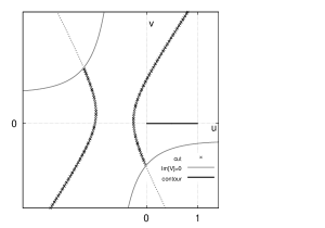
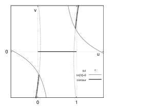
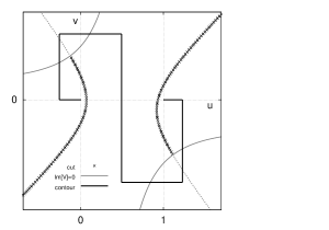
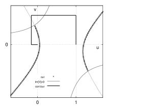
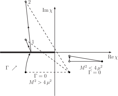
Different possibilities are illustrated in Fig. 2 where we show χ(x)𝜒𝑥\chi(x) for two equal (complex) internal masses.
Refer to caption
Figure 2: Analytical continuation from real p2superscript𝑝2p^{2} to complex p2superscript𝑝2p^{2} as seen in the χ𝜒\chi\,-plane with χ(x)=sPx(1x)+μ2iμγ𝜒𝑥subscript𝑠𝑃𝑥1𝑥superscript𝜇2𝑖𝜇𝛾\chi(x)=-s_{{\scriptscriptstyle{P}}}\,x\,(1-x)+\mu^{2}-i\,\mu\,\gamma, with sP=M2iMΓsubscript𝑠𝑃superscript𝑀2𝑖𝑀Γs_{{\scriptscriptstyle{P}}}=M^{2}-i\,M\,\Gamma and x[0,1]𝑥01x\in[0,1]. Solid lines represent the continuation for a low value of M𝑀M with a very small value for ΓΓ\Gamma. With increasing values for M𝑀M we reach the situation illustrated by the dot-lines, χ𝜒\chi moving into the second quadrant, i.e. χ𝜒\chi on the second Riemann sheet. Case 111 holds for Γ<(M/μ)γΓ𝑀𝜇𝛾\Gamma<(M/\mu)\,\gamma whereas case 222 holds for Γ>(M/μ)γΓ𝑀𝜇𝛾\Gamma>(M/\mu)\,\gamma. Black circles correspond to x=0,x=1formulae-sequence𝑥0𝑥1x=0,x=1 whereas white circles correspond to x=1/2𝑥12x=1/2.

In any realistic application the complex pole equation returns, for low values of M𝑀M, small values of ΓΓ\Gamma and ReχRe𝜒{\rm{Re}}\,\chi is always positive, never requiring analytical continuation into another sheet; when M𝑀M increases ΓΓ\Gamma increases too and we find values of χ𝜒\chi that requires the continuation lnlnsuperscript\ln\to\ln^{-}. This will happen for xI𝑥subscript𝐼x\geq I_{-} in case 111 (which requires Γ<(M/μ)γΓ𝑀𝜇𝛾\Gamma<(M/\mu)\,\gamma) and for x>R𝑥subscript𝑅x>R_{-} in case 222 (which requires Γ>(M/μ)γΓ𝑀𝜇𝛾\Gamma>(M/\mu)\,\gamma).

The same example can be discussed in the x𝑥x complex plane; in this case, when M>2μ𝑀2𝜇M>2\,\mu and Γ=γ=0Γ𝛾0\Gamma=\gamma=0, the cut is on the real axis between Rsubscript𝑅R_{-} and R+subscript𝑅R_{+} (Eq.(60)) and the integration is 0<x<1/20𝑥120<x<1/2. The integral is originally defined (Γ,γ=0Γ𝛾0\Gamma,\gamma=0) above the cut, i.e. for x+i 0𝑥𝑖 0x+i\,0. Analytical continuation means that for increasing imaginary parts we reach a point where the integration path is continued into the second Riemann sheet (at Γ=(M/μ)γΓ𝑀𝜇𝛾\Gamma=(M/\mu)\,\gamma, we have I=Rsubscript𝐼subscript𝑅I_{-}=R_{-} and, for higher values of ΓΓ\Gamma, the continuation to the second Riemann sheet is required as soon as the cut is reached). From this point of view the integral is better understood in terms of a variable z(x)=u+iv𝑧𝑥𝑢𝑖𝑣z(x)=u+i\,v, such that χ=M2z(1z)+μ2𝜒superscript𝑀2𝑧1𝑧superscript𝜇2\chi=-M^{2}\,z\,(1-z)+\mu^{2} and the integration is performed along the curve

v(12u)=ZM2,Z=μγMΓx(1x),u=1U2,U4+[4x(1x)1]U24Z2M4=0.formulae-sequence𝑣12𝑢𝑍superscript𝑀2formulae-sequence𝑍𝜇𝛾𝑀Γ𝑥1𝑥formulae-sequence𝑢1𝑈2superscript𝑈4delimited-[]4𝑥1𝑥1superscript𝑈24superscript𝑍2superscript𝑀40v\,(1\!-\!2\,u)=\frac{Z}{M^{2}},\qquad Z=\mu\,\gamma-M\Gamma\,x\,(1-x),\qquad u=\frac{1\!-\!U}{2},\qquad U^{4}+\Big{[}4\,x(1\!-\!x)-1\Big{]}\,U^{2}-4\,\frac{Z^{2}}{M^{4}}=0. (63)

Note that x=I𝑥subscript𝐼x=I_{-} corresponds to z=I𝑧subscript𝐼z=I_{-}, real. For real internal masses we have z(0)=0𝑧00z(0)=0 and z(1/2)=(Γ/(2M))1/2(1i/2)𝑧12superscriptΓ2𝑀121𝑖2z(1/2)=(\Gamma/(2M))^{1/2}\,(1-i/2). In the z𝑧z\,-plane the logarithm has a cut on the positive real axis between Rsubscript𝑅R_{-} and R+subscript𝑅R_{+}.

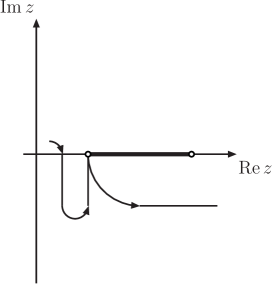
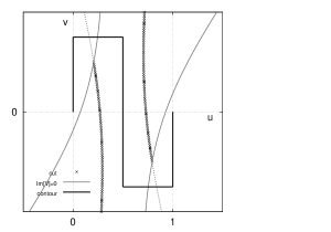
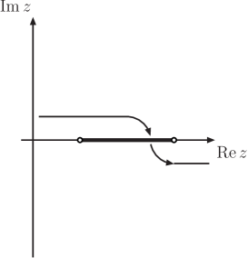
It is worth mentioning that case 222 of Fig. 2 corresponds to an integration path that crosses the cut of lnsuperscript\ln^{-} across the positive imaginary x𝑥x\,-axis, similar to the case of the dilogarithm discussed above. Therefore, the correct analytical continuation, for case 222, goes as follows: the integration path in z𝑧z\,-space (Eq.(63)) is moved into the complex plane and goes into the lower half-plane instead of reaching the cut of the logarithm (which is between Rsubscript𝑅R_{-} and R+subscript𝑅R_{+}, see also Fig. 3).

In order to insure that the analytically continued integral has a smooth limit Γ,γ0Γ𝛾0\Gamma,\gamma\to 0 we deform the integration path by insisting that the cut (of ln\ln) must be crossed at z=R𝑧subscript𝑅z=R_{-} (note that for case 222 we have I<Rsubscript𝐼subscript𝑅I_{-}<R_{-}) where we perform a continuation into the second Riemann sheet. In this way we add to B0subscript𝐵0B_{0} (on top of a factor  2iπβ2𝑖𝜋𝛽-\,2\,i\,\pi\,\beta) a new contribution which is easily computed in the x𝑥x\,-plane and it is related to the discontinuity of lnχ𝜒\ln\chi along a curve C𝐶C parametrized by

C(t):{x=1t2+if(t)},f(t)=12{ΓMt+[(1+Γ2M2)t2β2]1/2},:𝐶𝑡𝑥1𝑡2𝑖𝑓𝑡𝑓𝑡12Γ𝑀𝑡superscriptdelimited-[]1superscriptΓ2superscript𝑀2superscript𝑡2superscript𝛽212C(t)\;:\;\{x=\frac{1-t}{2}+i\,f(t)\},\qquad f(t)=\frac{1}{2}\,\Bigl{\{}-\,\frac{\Gamma}{M}\,t+\Bigl{[}\left(1+\frac{\Gamma^{2}}{M^{2}}\right)\,t^{2}-\beta^{2}\Bigr{]}^{1/2}\Bigr{\}}, (64)

with β2=14μ2/M2>0superscript𝛽214superscript𝜇2superscript𝑀20\beta^{2}=1-4\,\mu^{2}/M^{2}>0 and where β¯<t<β¯𝛽𝑡𝛽\bar{\beta}<t<\beta; here β¯¯𝛽\bar{\beta} is the value of t𝑡t where Reχ(t)=Imχ(t)=0Re𝜒𝑡Im𝜒𝑡0{\rm{Re}}\,\chi(t)={\rm{Im}}\chi(t)=0. The integral over C𝐶C is on the segment Reχ=±ϵRe𝜒plus-or-minusitalic-ϵ{\rm{Re}}\,\chi=\pm\epsilon with ϵ0+italic-ϵsuperscript0\epsilon\to 0^{+}, from μ2Γ/Mμγ>Imχ>0superscript𝜇2Γ𝑀𝜇𝛾Im𝜒0\mu^{2}\Gamma/M-\mu\gamma>{\rm{Im}}\chi>0 on the first Riemann sheet and from μ2Γ/Mμγ<Imχ<0superscript𝜇2Γ𝑀𝜇𝛾Im𝜒0\mu^{2}\Gamma/M-\mu\gamma<{\rm{Im}}\chi<0 on the second Riemann sheet. Therefore, we have to add to B0subscript𝐵0B_{0} an additional term  2iπΔA2𝑖𝜋Δ𝐴-\,2\,i\,\pi\,\Delta\,A with

ΔA=A(β¯)A(β),A(t)=(1+iΓM)ti[(1+Γ2M2)t2β2]1/2.formulae-sequenceΔ𝐴𝐴¯𝛽𝐴𝛽𝐴𝑡1𝑖Γ𝑀𝑡𝑖superscriptdelimited-[]1superscriptΓ2superscript𝑀2superscript𝑡2superscript𝛽212\Delta A=A(\bar{\beta})-A(\beta),\qquad A(t)=\left(1+i\,\frac{\Gamma}{M}\right)\,t-i\,\Bigl{[}\left(1+\frac{\Gamma^{2}}{M^{2}}\right)\,t^{2}-\beta^{2}\Bigr{]}^{1/2}. (65)

Note that in the limit Γ,γ0Γ𝛾0\Gamma,\gamma\to 0 we have β¯β¯𝛽𝛽\bar{\beta}\to\beta and this additional term vanishes. Furthermore, A(β)=β𝐴𝛽𝛽A(\beta)=\beta and A(β¯)=βc𝐴¯𝛽subscript𝛽𝑐A(\bar{\beta})=\beta_{c}, with βc2=14m2/spsubscriptsuperscript𝛽2𝑐14superscript𝑚2subscript𝑠𝑝\beta^{2}_{c}=1-4\,m^{2}/s_{p}. Therefore, we reproduce the correct result of Eq.(52). The recipe is, therefore, replace ln\ln with lnsuperscript\ln^{-} in the integrand but deform the integration contour in order to avoid crossing of the positive imaginary χ𝜒\chi\,-axis when this would occur.

In summary, our result with a simple example we observe that

LinAnalyt.Cont.Lin,Lin+1(z)0zdxxLin(x),\mbox{Li}_{n}\stackrel{{\scriptstyle\rm{\tiny{Analyt.Cont.}}}}{{\longmapsto}}\mbox{Li}^{-}_{n},\quad\mbox{Li}^{-}_{n+1}(z)\not=\int_{0}^{z}\,\frac{dx}{x}\,\mbox{Li}^{-}_{n}(x), (66)

since deformation of the integration contour is required for the general case.
Refer to caption
Refer to caption
Figure 3: Analytical continuation of a B0subscript𝐵0B_{0}\,-function as seen in the z𝑧z\,-plane with a cut along the positive real axis between Rsubscript𝑅R_{-} and R+subscript𝑅R_{+} (Eq.(60)). In the first part the integration path reaches the point Isubscript𝐼I_{-} (Eq.(60)) and continuation after z=I𝑧subscript𝐼z=I_{-} is in the second Riemann sheet. In the second part, where I<Rsubscript𝐼subscript𝑅I_{-}<R_{-} continuation must be, once again, in the second Riemann sheet; therefore the integration path which has moved into the lower half-plane must be deformed to cross the cut before moving once more into the lower half-plane (but on the second Riemann sheet).

6.5 Narrow width approximation

The practical implementation for higher point (or higher loop) functions presents a formidable technical problem, due to the higher dimension of the x𝑥x\,-space; more will be explained in Section 6.6 but, for this reason, we have also considered analytical continuation in narrow-width-approximation (hereafter NWA). Here we replace ln\ln with lnsuperscript\ln^{-} (or ln+superscript\ln^{+}) at the integrand level and do not perform any deformation of the integration (hyper-)contour. The resulting expression is expect to have a range of validity given by ΓMmuch-less-thanΓ𝑀\Gamma\ll M. Numerical investigation of the Higgs complex pole shows that NWA returns reliable results when compared with the exact expression. The rationale for analytical continuation in NWA is based on the fact that, as we are going to show, all higher-point (higher-loop) functions admit integral representations with integrand of logarithmic nature (one-loop) or, at most, of poly-logarithmic nature (multi-loop).

Consider now the extension to complex variables of an arbitrary scalar three-point function C0subscript𝐶0C_{0} (in NWA), defined by

C0=01𝑑x10x1𝑑x2V1ϵ/2(x1,x2),subscript𝐶0superscriptsubscript01differential-dsubscript𝑥1superscriptsubscript0subscript𝑥1differential-dsubscript𝑥2superscript𝑉1italic-ϵ2subscript𝑥1subscript𝑥2C_{0}=\int_{\scriptstyle 0}^{\scriptstyle 1}\,dx_{1}\,\int_{\scriptstyle 0}^{\scriptstyle x_{1}}\,dx_{2}\,V^{-1-\epsilon/2}(x_{1},x_{2}), (67)

where n=4ϵ𝑛4italic-ϵn=4-\epsilon and V𝑉V is a quadratic form

V(x1,x2)=ax12+bx22+cx1x2+dx1+ex2+fi 0xtHx+2Ktx+L,𝑉subscript𝑥1subscript𝑥2𝑎superscriptsubscript𝑥12𝑏superscriptsubscript𝑥22𝑐subscript𝑥1subscript𝑥2𝑑subscript𝑥1𝑒subscript𝑥2𝑓𝑖 0superscript𝑥𝑡𝐻𝑥2superscript𝐾𝑡𝑥𝐿V(x_{1},x_{2})=a\,x_{1}^{2}+b\,x_{2}^{2}+c\,x_{1}\,x_{2}+d\,x_{1}+e\,x_{2}+f-i\,0\equiv x^{t}\,H\,x+2\,K^{t}\,x+L, (68)

whose coefficients are related to the internal masses and the external momenta by the relations Hij=pipj,L=m12formulae-sequencesubscript𝐻𝑖𝑗subscript𝑝𝑖subscript𝑝𝑗𝐿subscriptsuperscript𝑚21H_{ij}=-\,{p_{i}}\cdot{p_{j}},L=m^{2}_{1} and

K1subscript𝐾1\displaystyle K_{1} =\displaystyle= 12(p1p1+m22m12),K2=12(PPp1p1+m32m22),12subscript𝑝1subscript𝑝1superscriptsubscript𝑚22superscriptsubscript𝑚12subscript𝐾212𝑃𝑃subscript𝑝1subscript𝑝1superscriptsubscript𝑚32superscriptsubscript𝑚22\displaystyle\frac{1}{2}\,({p_{1}}\cdot{p_{1}}+m_{2}^{2}-m_{1}^{2}),\quad K_{2}=\frac{1}{2}\,({P}\cdot{P}-{p_{1}}\cdot{p_{1}}+m_{3}^{2}-m_{2}^{2}), (69)

with P=p1+p2𝑃subscript𝑝1subscript𝑝2P=p_{1}+p_{2}. Let us define the usual Bernstein - Sato - Tkachov (hereafter BST) factors (see Ref. [27]) as B3=LKtH1Ksubscript𝐵3𝐿superscript𝐾𝑡superscript𝐻1𝐾B_{3}=L-K^{t}\,H^{-1}\,K and BST co-factors X=H1K𝑋superscript𝐻1𝐾X=-\,H^{-1}\,K. It is convenient to introduce special notations, X0=1,X3=0formulae-sequencesubscript𝑋01subscript𝑋30X_{0}=1,\,X_{3}=0, and V(ii+1^)𝑉^𝑖𝑖1V(\widehat{i\;i+1}) to denote contractions, i.e.

V(0 1^)=V(1,x1),V(1 2^)=V(x1,x1),V(2 3^)=V(x1,0).formulae-sequence𝑉^01𝑉1subscript𝑥1formulae-sequence𝑉^12𝑉subscript𝑥1subscript𝑥1𝑉^23𝑉subscript𝑥10V(\widehat{0\;1})=V(1,x_{1}),\quad V(\widehat{1\;2})=V(x_{1},x_{1}),\quad V(\widehat{2\;3})=V(x_{1},0). (70)

In this way we obtain a simple integral representation

C0=1B3{12+01dx1[0x1dx2lnV(x1,x2)12i=02(XiXi+1)lnV(ii+1^).]}.C_{0}=\frac{1}{B_{3}}\,\Bigl{\{}\frac{1}{2}+\int_{0}^{1}\,dx_{1}\,\Bigl{[}\int_{0}^{x_{1}}\,dx_{2}\,\ln\,V(x_{1},x_{2})-\frac{1}{2}\,\sum_{i=0}^{2}\,(X_{i}-X_{i+1})\,\ln V(\widehat{i\;i+1}).\Bigr{]}\Bigr{\}}. (71)

When some or all the invariants are complex, P2=sPsuperscript𝑃2subscript𝑠𝑃P^{2}=-\,s_{{\scriptscriptstyle{P}}} with sP=M2iΓMsubscript𝑠𝑃superscript𝑀2𝑖Γ𝑀s_{{\scriptscriptstyle{P}}}=M^{2}-i\,\Gamma\,M and mi2=μi2iγiμisubscriptsuperscript𝑚2𝑖subscriptsuperscript𝜇2𝑖𝑖subscript𝛾𝑖subscript𝜇𝑖m^{2}_{i}=\mu^{2}_{i}-i\,\gamma_{i}\,\mu_{i} (in realistic cases, e.g. decay of an unstable particle, p1,22subscriptsuperscript𝑝212p^{2}_{1,2} are real) we define

V=V|Γ,γi=0,subscript𝑉evaluated-at𝑉Γsubscript𝛾𝑖0V_{-}=V\Bigr{|}_{\Gamma,\gamma_{i}=0}, (72)

which includes the i 0𝑖 0-\,i\,0 prescription and write

C0subscript𝐶0\displaystyle C_{0} =\displaystyle= 1B3{12+01dx1[0x1dx2ln(V(x1,x2);V(x1,x2))\displaystyle\frac{1}{B_{3}}\,\Bigl{\{}\frac{1}{2}+\int_{0}^{1}\,dx_{1}\,\Bigl{[}\int_{0}^{x_{1}}\,dx_{2}\,\ln^{-}\left(V(x_{1},x_{2})\,;\,V_{-}(x_{1},x_{2})\right) (73)
\displaystyle- 12i=02(XiXi+1)ln(V(ii+1^);V(ii+1^))]}.\displaystyle\frac{1}{2}\,\sum_{i=0}^{2}\,(X_{i}-X_{i+1})\,\ln^{-}\left(V(\widehat{i\;i+1})\,;\,V_{-}(\widehat{i\;i+1})\right)\Bigr{]}\Bigr{\}}.

For instance, with P2=M2+iMΓsuperscript𝑃2superscript𝑀2𝑖𝑀ΓP^{2}=-M^{2}+i\,M\,\Gamma, p1,22=0subscriptsuperscript𝑝2120p^{2}_{1,2}=0 and m1,3=0subscript𝑚130m_{1,3}=0, m22=μ2iμγsubscriptsuperscript𝑚22superscript𝜇2𝑖𝜇𝛾m^{2}_{2}=\mu^{2}-i\,\mu\,\gamma we find that when Γ/γμ/MΓ𝛾𝜇𝑀\Gamma/\gamma\leq\mu/M lnV𝑉\ln V must be continued to the second Riemann sheet for 0x2(μγ)/(MΓ)0subscript𝑥2𝜇𝛾𝑀Γ0\leq x_{2}\leq(\mu\gamma)/(M\Gamma).

Starting with an integral representation of a three-point function where the integrand is the logarithm of a polynomial in parametric space is the safest way of performing analytical continuation; of course, going beyond NWA requires contour deformation but even the latter admits a consistent numerical implementation. Nor should one fail to notice ’t Hooft and Veltman emphasis, in their seminal work [29], on this subject: they put up warning signs about continuation of their result to complex momenta.

For higher point functions (L=D,E,F,𝐿𝐷𝐸𝐹L=D,E,F,\,\dots) we apply the BST algorithm [30] as many times as it is needed to produce logarithms in the integrand and proceed by replacing ln\ln with lnsuperscript\ln^{-},

L={x}d{x}ln(χ({x})i 0){x}C(χ)d{x}lnχ({x}),𝐿subscript𝑥𝑑𝑥𝜒𝑥𝑖 0subscriptsubscript𝑥𝐶𝜒𝑑𝑥superscript𝜒𝑥L=\int_{\{x\}}d\{x\}\,\ln\left(\chi(\{x\})-i\,0\right)\to\int_{\{x\}_{C(\chi)}}d\{x\}\,\ln^{-}\,\chi(\{x\}), (74)

where {x}𝑥\{x\} is the x1,,xnsubscript𝑥1subscript𝑥𝑛x_{1},\,\dots\,,x_{n} simplex and {x}C(χ)subscript𝑥𝐶𝜒\{x\}_{C(\chi)} is the path that avoids crossing the positive imaginary χ𝜒\chi\,-axis. NWA amounts to the identification {x}C(χ){x}subscript𝑥𝐶𝜒𝑥\{x\}_{C(\chi)}\equiv\{x\}.

For multi-loop integrals other functions must be extended, e.g. we will use Eq.(53), with similar results for all generalized Nielsen polylogarithms [26]

Sn,p(zUST;zST)=Sn,p(zUST)+k=1p(2iπ)kk![Sn,pk(zUST)j=0n1lnjzUSTj!Snj,pk(zUST)]θ(zRUST1)θ(zIUST),subscriptsuperscript𝑆𝑛𝑝superscript𝑧USTsubscriptsuperscript𝑧STsubscript𝑆𝑛𝑝superscript𝑧USTsuperscriptsubscript𝑘1𝑝superscript2𝑖𝜋𝑘𝑘delimited-[]subscript𝑆𝑛𝑝𝑘superscript𝑧USTsuperscriptsubscript𝑗0𝑛1superscript𝑗superscript𝑧UST𝑗subscript𝑆𝑛𝑗𝑝𝑘superscript𝑧UST𝜃subscriptsuperscript𝑧UST𝑅1𝜃subscriptsuperscript𝑧UST𝐼S^{-}_{n,p}(z^{\!\rm{\scriptscriptstyle{UST}}}\!;\!z^{\rm{\scriptscriptstyle{ST}}}_{-})=\,S_{n,p}(z^{\!\rm{\scriptscriptstyle{UST}}})\,+\,\sum_{k=1}^{p}\frac{(-2i\pi)^{\!k}}{k\,!}\bigg{[}S_{n,p-k}(z^{\!\rm{\scriptscriptstyle{UST}}})\,-\sum_{j=0}^{n-1}\frac{\ln^{j}\!z^{\!\rm{\scriptscriptstyle{UST}}}\!}{j\,!}S_{n-j,p-k}(z^{\!\rm{\scriptscriptstyle{UST}}})\bigg{]}\theta(z^{\!\rm{\scriptscriptstyle{UST}}}_{{\scriptscriptstyle{R}}}\!-\!1)\,\theta(z^{\!\rm{\scriptscriptstyle{UST}}}_{{\scriptscriptstyle{I}}}), (75)

which is derived by using ln+superscript\ln^{+} in the integral representation of the generalized Nielsen polylogarithms. Since it has been shown that multi-loop diagrams can be written as integrals of multivariate generalized Nielsen polylogarithms [31] our recipe gives the analytical continuation to all orders in perturbation theory, but one does have to be careful in one respect: using familiar relations such as splitting of logarithms should be done with a grain of salt.

6.6 Analytical continuation and contour deformation

Exact analytical continuation at the integrand level can be performed by deforming the integration contour into the complex parametric space (for a general treatment see Ref. [28]). In this case we need the general definition of lnsuperscript\ln^{-} given in Eq.(37).

To illustrate contour deformation we consider, once again, the case of a B0subscript𝐵0B_{0}\,-function with equal (complex) internal masses. If

M>2μμΓMγ>0,formulae-sequence𝑀2𝜇𝜇Γ𝑀𝛾0M>2\,\mu\qquad\mu\,\Gamma-M\,\gamma>0, (76)

the function χ(x),x[0,12]𝜒𝑥𝑥012\chi(x),x\in[0,\frac{1}{2}] crosses the positive imaginary axis (the branch cut of lnsuperscript\ln^{-}). To avoid crossing we deform the x𝑥x\,-integration into

1)\displaystyle 1)\quad x=iΓMβt,𝑥𝑖Γ𝑀𝛽𝑡\displaystyle\quad x=i\,\frac{\Gamma}{M}\,\beta\,t,
2)\displaystyle 2)\quad x=12t+iΓMβ(1t),𝑥12𝑡𝑖Γ𝑀𝛽1𝑡\displaystyle\quad x=\frac{1}{2}\,t+i\,\frac{\Gamma}{M}\,\beta\,(1-t), (77)

with t[0,1]𝑡01t\in[0,1] and β𝛽\beta a free parameter. For χ(1)superscript𝜒1\chi^{(1)} we require Imχ(1)(t)<0,t[0,1]formulae-sequenceImsuperscript𝜒1𝑡0for-all𝑡01{\rm{Im}}\,\chi^{(1)}(t)<0,\forall t\in[0,1]; this is possible if β<βmax𝛽subscript𝛽max\beta<\beta_{\rm max}, with

βmax=12M2Γ2[1+1+4μγΓM3].subscript𝛽max12superscript𝑀2superscriptΓ2delimited-[]114𝜇𝛾Γsuperscript𝑀3\beta_{\rm max}=\frac{1}{2}\,\frac{M^{2}}{\Gamma^{2}}\,\Bigl{[}1+\sqrt{1+4\,\frac{\mu\,\gamma\,\Gamma}{M^{3}}}\Bigr{]}. (78)

For χ(2)superscript𝜒2\chi^{(2)} we require that Reχ(2)(t)=0Resuperscript𝜒2𝑡0{\rm{Re}}\,\chi^{(2)}(t)=0 corresponds to Imχ(2)(t)<0Imsuperscript𝜒2𝑡0{\rm{Im}}\,\chi^{(2)}(t)<0, which requires β>βmin𝛽subscript𝛽min\beta>\beta_{\rm min}, where βminsubscript𝛽min\beta_{\rm min} is the largest, real, solution of the following equation

μ(ΓM214Γ)(ΓμMγ)(β21)+[14(M2+Γ2)μ(μ+ΓγM)]β=0.𝜇Γsuperscript𝑀214ΓΓ𝜇𝑀𝛾superscript𝛽21delimited-[]14superscript𝑀2superscriptΓ2𝜇𝜇Γ𝛾𝑀𝛽0\mu\,\left(\frac{\Gamma}{M^{2}}-\frac{1}{4\,\Gamma}\right)\,\left(\Gamma\,\mu-M\,\gamma\right)\,(\beta^{2}-1)+\Bigl{[}\frac{1}{4}\,\left(M^{2}+\Gamma^{2}\right)-\mu\,\left(\mu+\frac{\Gamma\,\gamma}{M}\right)\,\Bigr{]}\,\beta=0. (79)

For βmin<β<βmaxsubscript𝛽min𝛽subscript𝛽max\beta_{\rm min}<\beta<\beta_{\rm max} we have that χ(1,2)superscript𝜒12\chi^{(1,2)} never cross the positive imaginary axis. Furthermore, we compare χ(1,2)(0)superscript𝜒120\chi^{(1,2)}(0) with χ(1,2)(Γ)superscript𝜒12Γ\chi^{(1,2)}(\Gamma) at fixed t[0,1]𝑡01t\in[0,1] and replace lnlnsuperscript\ln\to\ln^{-} when (always at fixed t𝑡t) χ(1,2)(Γ)superscript𝜒12Γ\chi^{(1,2)}(\Gamma) crosses the negative real axis for some value ΓcsubscriptΓ𝑐\Gamma_{c}. In the example that we are considering, illustrated in Fig. 4, everything is particularly simple since Imχ(Reχ)Im𝜒Re𝜒{\rm{Im}}\,\chi({\rm{Re}}\,\chi) is always a straight line but our recipe works, as well, in the general case and allows for a straightforward algorithmic implementation.
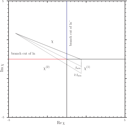
Refer to caption
Figure 4: Example of contour deformations in computing a scalar two-point functions with equal (complex) internal masses and complex p2superscript𝑝2p^{2}.

For a general recipe of contour deformation, we proceed by analyzing the case where a Feynman diagram can be written as:

01𝑑x1𝑑xniAi(x1,,xn)lnVi(x1,,xn),superscriptsubscript01differential-dsubscript𝑥1differential-dsubscript𝑥𝑛subscript𝑖subscript𝐴𝑖subscript𝑥1subscript𝑥𝑛subscript𝑉𝑖subscript𝑥1subscript𝑥𝑛\int_{0}^{1}\!\!dx_{1}\cdots dx_{n}\,\sum_{i}\,A_{i}(x_{1},\dots,x_{n})\,\ln V_{i}(x_{1},\dots,x_{n}), (80)

where Visubscript𝑉𝑖V_{i} are multivariate polynomials in x1,,xnsubscript𝑥1subscript𝑥𝑛x_{1},\dots,x_{n}, at most quadratic in each variable (note that all one-loop diagrams can be written according to Eq.(80), see Ref. [27]); actually the procedure works as well when each Visubscript𝑉𝑖V_{i} is a quadratic form in, at least, one variable. For each term in the sum, we select one variable xxi𝑥subscript𝑥𝑖x\equiv x_{i} (among x1,,xnsubscript𝑥1subscript𝑥𝑛x_{1},\dots,x_{n}) and study the analytical continuation (assuming that Im[V]realmasses<0Imsubscriptdelimited-[]𝑉realmasses0{\rm Im}[V]_{\rm real\;masses}<0)

lnVlnV with V=ax2+bx+c,formulae-sequence𝑉superscript𝑉 with 𝑉𝑎superscript𝑥2𝑏𝑥𝑐\ln V\to\ln^{-}V\qquad\mbox{ with }\qquad V=a\,x^{2}+b\,x+c, (81)

where a,b,c𝑎𝑏𝑐a,b,c are polynomials in the remaining Feynman variables. The idea is to deform only the x𝑥x integration contour into the complex plane (when needed) while keeping all other variables (x1,,xi1,xi+1,,xnsubscript𝑥1subscript𝑥𝑖1subscript𝑥𝑖1subscript𝑥𝑛x_{1},\dots,x_{i-1},x_{i+1},\dots,x_{n}) on the real axis. We define

a=ar+iaib=br+ibic=cr+icix=u+iv.formulae-sequence𝑎subscript𝑎𝑟𝑖subscript𝑎𝑖formulae-sequence𝑏subscript𝑏𝑟𝑖subscript𝑏𝑖formulae-sequence𝑐subscript𝑐𝑟𝑖subscript𝑐𝑖𝑥𝑢𝑖𝑣a=a_{r}+i\,a_{i}\qquad b=b_{r}+i\,b_{i}\qquad c=c_{r}+i\,c_{i}\qquad\quad x=u+i\,v. (82)

The real and imaginary parts of V𝑉V are then given by:

ReVRe𝑉\displaystyle{\rm Re}V =\displaystyle= aru22,aiuvarv2+brubiv+crsubscript𝑎𝑟superscript𝑢22subscript𝑎𝑖𝑢𝑣subscript𝑎𝑟superscript𝑣2subscript𝑏𝑟𝑢subscript𝑏𝑖𝑣subscript𝑐𝑟\displaystyle a_{r}\,u^{2}-2,a_{i}\,u\,v-a_{r}\,v^{2}+b_{r}\,u-b_{i}\,v+c_{r}
=\displaystyle= ar(uuc)22ai(uuc)(vvc)ar(vvc)2+δr,subscript𝑎𝑟superscript𝑢subscript𝑢𝑐22subscript𝑎𝑖𝑢subscript𝑢𝑐𝑣subscript𝑣𝑐subscript𝑎𝑟superscript𝑣subscript𝑣𝑐2subscript𝛿𝑟\displaystyle a_{r}\,(u-u_{c})^{2}-2\,a_{i}\,(u-u_{c})\,(v-v_{c})-a_{r}\,(v-v_{c})^{2}+\delta_{r},
ImVIm𝑉\displaystyle{\rm Im}V =\displaystyle= aiu2+2,aruvaiv2+biu+brv+cisubscript𝑎𝑖superscript𝑢22subscript𝑎𝑟𝑢𝑣subscript𝑎𝑖superscript𝑣2subscript𝑏𝑖𝑢subscript𝑏𝑟𝑣subscript𝑐𝑖\displaystyle a_{i}\,u^{2}+2,a_{r}\,u\,v-a_{i}\,v^{2}+b_{i}\,u+b_{r}\,v+c_{i} (83)
=\displaystyle= ai(uuc)2+2ar(uuc)(vvc)ai(vvc)2+δi,subscript𝑎𝑖superscript𝑢subscript𝑢𝑐22subscript𝑎𝑟𝑢subscript𝑢𝑐𝑣subscript𝑣𝑐subscript𝑎𝑖superscript𝑣subscript𝑣𝑐2subscript𝛿𝑖\displaystyle a_{i}\,(u-u_{c})^{2}+2\,a_{r}\,(u-u_{c})\,(v-v_{c})-a_{i}\,(v-v_{c})^{2}+\delta_{i},

where we introduced the following auxiliary variables:

xc=uc+ivc=ab2|a|2,δ=δr+iδi=cab24|a|2.formulae-sequencesubscript𝑥𝑐subscript𝑢𝑐𝑖subscript𝑣𝑐superscript𝑎𝑏2superscript𝑎2𝛿subscript𝛿𝑟𝑖subscript𝛿𝑖𝑐superscript𝑎superscript𝑏24superscript𝑎2x_{c}=u_{c}+i\,v_{c}=-\,\frac{a^{*}\,b}{2\,|a|^{2}},\qquad\qquad\delta=\delta_{r}+i\,\delta_{i}=c-\frac{a^{*}\,b^{2}}{4\,|a|^{2}}. (84)

The curves ReV=0Re𝑉0{\rm Re}V=0 and ImV=0Im𝑉0{\rm Im}V=0 are hyperbolas with center in xcsubscript𝑥𝑐x_{c}. We also define an auxiliary function,

U=aiReV+arImV=2|a|2(uuc)(vvc)+arδiaiδr.𝑈subscript𝑎𝑖Re𝑉subscript𝑎𝑟Im𝑉2superscript𝑎2𝑢subscript𝑢𝑐𝑣subscript𝑣𝑐subscript𝑎𝑟subscript𝛿𝑖subscript𝑎𝑖subscript𝛿𝑟U=-a_{i}\,{\rm Re}V+a_{r}\,{\rm Im}V=2\,|a|^{2}\,(u-u_{c})\,(v-v_{c})+a_{r}\,\delta_{i}-a_{i}\,\delta_{r}. (85)

The curve U=0𝑈0U=0 is again an hyperbola with center in xcsubscript𝑥𝑐x_{c} and asymptotes parallel to the u𝑢u and v𝑣v axes. The branch-cut of lnVsuperscript𝑉\ln^{-}V in the x𝑥x complex plane is defined by:

cut:ReV=0&ImV0{ReV=0&U0, if ar>0,ReV=0&U0, if ar<0.\mbox{cut}:\qquad{\rm Re}V=0\;\,\&\,\;{\rm Im}V\geq 0\qquad\Longleftrightarrow\qquad\left\{\begin{array}[]{c}{\rm Re}V=0\;\,\&\,\;U\geq 0,\quad\mbox{ if }a_{r}>0,\\ {\rm Re}V=0\;\,\&\,\;U\leq 0,\quad\mbox{ if }a_{r}<0.\end{array}\right. (86)

First we study the intersection of the curve ReV=0Re𝑉0{\rm Re}V=0 with the real u𝑢u\, axis. If Δ=br24arcr<0Δsuperscriptsubscript𝑏𝑟24subscript𝑎𝑟subscript𝑐𝑟0\Delta=b_{r}^{2}-4\,a_{r}\,c_{r}<0, the hyperbola ReV=0Re𝑉0{\rm Re}V=0 never crosses the real axis and there is no need of contour deformation (this is the first case of Fig. 5).
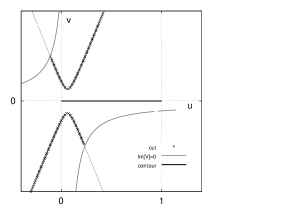
Refer to caption Refer to caption Refer to caption
Figure 5: Examples of deformation in the x𝑥x-complex plane (x=u+iv𝑥𝑢𝑖𝑣x=u+iv) of the integration contour [0,1]01[0,1] for integral of lnV=ln(ax2+bx+c)superscript𝑉superscript𝑎superscript𝑥2𝑏𝑥𝑐\ln^{-}V=\ln^{-}(ax^{2}+bx+c).

If Δ0Δ0\Delta\geq 0, the intersections are given by:

ReV=0&v=0u=u0±=br±Δ2ar.formulae-sequenceRe𝑉0𝑣0𝑢superscriptsubscript𝑢0plus-or-minusplus-or-minussubscript𝑏𝑟Δ2subscript𝑎𝑟{\rm Re}V=0\;\,\&\,\;v=0\qquad\Longrightarrow\qquad u=u_{0}^{\pm}=\frac{-b_{r}\pm\sqrt{\Delta}}{2\,a_{r}}. (87)

If both solutions are not in [0,1]01[0,1] a distortion is not needed (second plot in Fig. 5). Even if u0±[0,1]superscriptsubscript𝑢0plus-or-minus01u_{0}^{\pm}\in[0,1], it can happen that the intersection occurs for ImV<0Im𝑉0{\rm Im}V<0 (as in the third case of Fig. 5) and there is no need of deformation to avoid the cut. In order to understand whether it occurs, we can study where the zeros of V𝑉V (ReV=ImV=0Re𝑉Im𝑉0{\rm Re}V={\rm Im}V=0) are lying. This system of equations has always two and only two solutions x±=u±+iv±subscript𝑥plus-or-minussubscript𝑢plus-or-minus𝑖subscript𝑣plus-or-minusx_{\pm}=u_{\pm}+i\,v_{\pm}, whose real and imaginary parts are given by:

u±=uc±|σ|+σr,v±=vc±sign(σi)|σ|σr,σ=aδ2|a|2.formulae-sequencesubscript𝑢plus-or-minusplus-or-minussubscript𝑢𝑐𝜎subscript𝜎𝑟formulae-sequencesubscript𝑣plus-or-minusplus-or-minussubscript𝑣𝑐signsubscript𝜎𝑖𝜎subscript𝜎𝑟𝜎superscript𝑎𝛿2superscript𝑎2u_{\pm}=u_{c}\pm\sqrt{|\sigma|+\sigma_{r}},\qquad\quad v_{\pm}=v_{c}\pm\,{\rm{sign}}\left({\sigma_{i}}\right)\sqrt{|\sigma|-\sigma_{r}},\qquad\qquad\sigma=-\,\frac{a^{*}\,\delta}{2\,|a|^{2}}. (88)

Note that these points are also solution of the equation U=0𝑈0U=0 and (because of the simple form of U𝑈U) we can conclude that:

cut:ReV=0&ImV0{ReV=0&U0ReV=0&{vv+ if u>ucvv if u<uc if ar>0,ReV=0&U0ReV=0&{vv+ if u>ucvv if u<uc if ar<0.:cutRe𝑉0Im𝑉0casesRe𝑉0𝑈0Re𝑉0cases𝑣subscript𝑣 if 𝑢subscript𝑢𝑐𝑣subscript𝑣 if 𝑢subscript𝑢𝑐 if subscript𝑎𝑟0Re𝑉0𝑈0Re𝑉0cases𝑣subscript𝑣 if 𝑢subscript𝑢𝑐𝑣subscript𝑣 if 𝑢subscript𝑢𝑐 if subscript𝑎𝑟0\mbox{cut}\!:\;\;{\rm Re}V\!=0\;\,\&\,\;{\rm Im}V\geq 0\;\;\Leftrightarrow\,\left\{\begin{array}[]{c}{\rm Re}V\!=0\;\,\&\,\;U\geq 0\;\;\Leftrightarrow\;\;{\rm Re}V\!=0\;\,\&\left\{\begin{array}[]{c}v\geq v_{+}\;\mbox{ if }\;u\!>\!u_{c}\\ v\leq v_{-}\;\mbox{ if }\;u\!<\!u_{c}\\ \end{array}\right.\;\mbox{ if }a_{r}\!>\!0,\\ {\rm Re}V\!=0\;\,\&\,\;U\leq 0\;\;\Leftrightarrow\;\;{\rm Re}V\!=0\;\,\&\left\{\begin{array}[]{c}v\leq v_{+}\;\mbox{ if }\;u\!>\!u_{c}\\ v\geq v_{-}\;\mbox{ if }\;u\!<\!u_{c}\\ \end{array}\right.\;\mbox{ if }a_{r}\!<\!0.\end{array}\right. (89)

At this point we have all information to fix the new integration contour, starting from x=0𝑥0x=0 and ending at x=1𝑥1x=1 without crossing the branch-cut. Of course, as long as the cut is not crossed, all integration contours are equivalent and give the same result: it may fairly be said that we have some freedom in defining the deformation and that, at the same time, we can control the correctness of the result by using different paths. The general situation is depicted in the fourth plot of Fig. 5 and the new integration contour is defined by seven segments:

(1)1\displaystyle(1) x=α1t,𝑥subscript𝛼1𝑡\displaystyle x\,=\,-\alpha_{1}\,t,
(2)2\displaystyle(2) x=α1+iβ1t,𝑥subscript𝛼1𝑖subscript𝛽1𝑡\displaystyle x\,=\,-\alpha_{1}+i\,\beta_{1}\,t,
(3)3\displaystyle(3) x=α1(1t)+αct+iβ1,𝑥subscript𝛼11𝑡subscript𝛼𝑐𝑡𝑖subscript𝛽1\displaystyle x\,=\,-\alpha_{1}\,(1-t)+\alpha_{c}\,t+i\,\beta_{1},
(4)4\displaystyle(4) x=αc+iβ1(1t)+β2t,𝑥subscript𝛼𝑐𝑖subscript𝛽11𝑡subscript𝛽2𝑡\displaystyle x\,=\,\alpha_{c}+i\,\beta_{1}\,(1-t)+\beta_{2}\,t,
(5)5\displaystyle(5) x=αc(1t)+(1+α2)t+iβ2,𝑥subscript𝛼𝑐1𝑡1subscript𝛼2𝑡𝑖subscript𝛽2\displaystyle x\,=\,\alpha_{c}\,(1-t)+(1+\alpha_{2})\,t+i\,\beta_{2},
(6)6\displaystyle(6) x= 1+α2+iβ2(1t),𝑥1subscript𝛼2𝑖subscript𝛽21𝑡\displaystyle x\,=\,1+\alpha_{2}+i\,\beta_{2}\,(1-t),
(7)7\displaystyle(7) x=(1+α2)(1t)+t.𝑥1subscript𝛼21𝑡𝑡\displaystyle x\,=\,(1+\alpha_{2})\,(1-t)+t. (90)

The coefficients α1subscript𝛼1\alpha_{1}, β1subscript𝛽1\beta_{1}, α2subscript𝛼2\alpha_{2}, β1subscript𝛽1\beta_{1} and αcsubscript𝛼𝑐\alpha_{c} can be fixed according to the principle of the minimal deformation to avoid crossing the cut. This gives the following conditions:

α1>|u|if0u01&u0,α1=0otherwise,{β1>|v|β1<|v|if0u01&v0&ar>0,v0&ar<0,β1=0otherwise,α2>|u+|if0u0+1&u+1,α2=0otherwise,{β2<|v+|β2>|v+|if0u0+1&v+0&ar>0,v+0&ar<0,β2=0otherwise,{αc=ucαc=     0αc=     1if0u0u0+1,u00u0+1,0u01u0+,αc=0otherwise.\displaystyle\begin{array}[]{lccccl}\;\;\;\alpha_{1}>\;\;\;|u_{-}|&\quad{\rm if}&0\leq u_{0}^{-}\leq 1&\quad\,\&&u_{-}\leq 0,&\qquad\alpha_{1}=0\quad{\rm otherwise},\\[5.69046pt] \left\{\begin{array}[]{l}\beta_{1}>\;\;\;|v_{-}|\\ \beta_{1}<-\,|v_{-}|\end{array}\right.&\quad{\rm if}&0\leq u_{0}^{-}\leq 1&\quad\,\&&\begin{array}[]{l}v_{-}\geq 0\;\,\&\,\;a_{r}>0,\\ v_{-}\leq 0\;\,\&\,\;a_{r}<0,\end{array}&\qquad\beta_{1}=0\quad{\rm otherwise},\\[11.38092pt] \;\;\;\alpha_{2}>\;\;\;|u_{+}|&\quad{\rm if}&0\leq u_{0}^{+}\leq 1&\quad\,\&&u_{+}\geq 1,&\qquad\alpha_{2}=0\quad{\rm otherwise},\\[5.69046pt] \left\{\begin{array}[]{ll}\beta_{2}<-\,|v_{+}|\\ \beta_{2}>\;\;\;|v_{+}|\end{array}\right.&\quad{\rm if}&0\leq u_{0}^{+}\leq 1&\quad\,\&&\begin{array}[]{ll}v_{+}\leq 0\;\,\&\,\;a_{r}>0,\\ v_{+}\geq 0\;\,\&\,\;a_{r}<0,\end{array}&\qquad\beta_{2}=0\quad{\rm otherwise},\\[11.38092pt] \left\{\begin{array}[]{ll}\alpha_{c}=\;\;\;\;u_{c}\\ \alpha_{c}=\;\;\;\;\;0\\ \alpha_{c}=\;\;\;\;\;1\\ \end{array}\right.&\quad{\rm if}&\begin{array}[]{l}0\leq u_{0}^{-}\leq u_{0}^{+}\leq 1,\\ u_{0}^{-}\leq 0\leq u_{0}^{+}\leq 1,\\ 0\leq u_{0}^{-}\leq 1\leq u_{0}^{+},\end{array}&&&\qquad\alpha_{c}=0\quad{\rm otherwise}.\end{array} (110)

The case where all coefficients vanish corresponds to non-deformation: in this case the paths in Eq.(90) are

(1),(2),(3),(4)x=0,(5)x=t,(6),(7)x=1,formulae-sequence1234𝑥0formulae-sequence5𝑥𝑡67𝑥1(1),\,(2),\,(3),\,(4)\;\;x=0,\quad(5)\;\;x=t,\quad(6),\,(7)\;\;x=1, (111)

and refer to 0x10𝑥10\leq x\leq 1 on the real axis. Note that the case Δ<0Δ0\Delta<0 (where u0±superscriptsubscript𝑢0plus-or-minusu_{0}^{\pm} are not defined) belongs to this class. This general recipe for contour deformation works also in special cases where not all segments are needed. For example, in the fifth plot of Fig. 5 the new contour consists of only four segments: using in Eq.(90) the conditions of Eq.(110) (α2=β2=0,αc=1formulae-sequencesubscript𝛼2subscript𝛽20subscript𝛼𝑐1\alpha_{2}=\beta_{2}=0,\alpha_{c}=1), the last three segments reduce in this case to the point x=1𝑥1x=1.

We can now consider in this framework the example of a B0subscript𝐵0B_{0} function with two equal masses. In this case we have:

V(x)=sPx(1x)+m2=(M2+iMΓ)x(1x)+μ2iμγ,𝑉𝑥subscript𝑠𝑃𝑥1𝑥superscript𝑚2superscript𝑀2𝑖𝑀Γ𝑥1𝑥superscript𝜇2𝑖𝜇𝛾V(x)=-s_{\scriptscriptstyle{P}}\,x\,(1-x)+m^{2}=(-M^{2}+i\,M\,\Gamma)\,x\,(1-x)+\mu^{2}-i\,\mu\,\gamma, (112)

which corresponds to

xc=12,δ=ca4=μ2M22i[μγ+MΓ2],formulae-sequencesubscript𝑥𝑐12𝛿𝑐𝑎4superscript𝜇2superscript𝑀22𝑖delimited-[]𝜇𝛾𝑀Γ2\displaystyle x_{c}=\frac{1}{2},\qquad\quad\delta=c-\frac{a}{4}=\mu^{2}-\frac{M^{2}}{2}-i\,\Big{[}\mu\,\gamma+\frac{M\,\Gamma}{2}\Big{]},
σ=18ac2|a|2=18μ2MμM+γΓM2+Γ2+iμ2MμΓMγM2+Γ2.𝜎18superscript𝑎𝑐2superscript𝑎218𝜇2𝑀𝜇𝑀𝛾Γsuperscript𝑀2superscriptΓ2𝑖𝜇2𝑀𝜇Γ𝑀𝛾superscript𝑀2superscriptΓ2\displaystyle\sigma=\frac{1}{8}-\frac{a^{*}c}{2|a|^{2}}=\frac{1}{8}-\frac{\mu}{2M}\frac{\mu M+\gamma\Gamma}{M^{2}+\Gamma^{2}}+i\frac{\mu}{2M}\frac{\mu\Gamma-M\gamma}{M^{2}+\Gamma^{2}}. (113)

Since ar>0subscript𝑎𝑟0a_{r}>0, the cut crosses the segment [0,1]01[0,1] when σi0subscript𝜎𝑖0\sigma_{i}\leq 0 (implying that v0subscript𝑣0v_{-}\geq 0, v+0subscript𝑣0v_{+}\leq 0), a situation which occurs for μΓMγ0𝜇Γ𝑀𝛾0\mu\Gamma-M\gamma\geq 0. It can be verified by explicit calculation that, in this case, we always have 0u±10subscript𝑢plus-or-minus10\leq u_{\pm}\leq 1, which corresponds to the situation depicted in the last diagram of Fig. 5 and the deformation requires five segments (α1=α2=0subscript𝛼1subscript𝛼20\alpha_{1}=\alpha_{2}=0, i.e. the first and the last segment in Eq.(90) reduce to a point).

6.7 Differential operators in a complex domain

The procedure of analytical continuation at the basis of Eq.(80) deserves an additional comment: how can we apply a differential operator at the integrand level, in order to get Eq.(80)? As an example we consider the integral of Eq.(67) on which we want to apply the BST algorithm:

C0=01𝑑x0x𝑑yχ1+ϵ/2(x,y),ϵ0+,formulae-sequencesubscript𝐶0superscriptsubscript01differential-d𝑥superscriptsubscript0𝑥differential-d𝑦superscript𝜒1italic-ϵ2𝑥𝑦italic-ϵsuperscript0C_{0}=\int_{\scriptstyle 0}^{\scriptstyle 1}\,dx\,\int_{\scriptstyle 0}^{\scriptstyle x}\,dy\,\chi^{-1+\epsilon/2}(x,y),\qquad\epsilon\to 0^{+}, (114)

where χ𝜒\chi is a quadratic form. As we know Eq.(80) follows from BST functional relation; in order to apply the BST algorithm in the complex domain (χC[x,y]𝜒𝐶𝑥𝑦\chi\in C[x,y]) we introduce

[χ]±μ=exp(μln±χ),superscriptsubscriptdelimited-[]𝜒plus-or-minus𝜇𝜇superscriptplus-or-minus𝜒\Bigl{[}\chi\Bigr{]}_{\pm}^{\mu}=\exp\left(\mu\,\ln^{\pm}\,\chi\right), (115)

and distort the integration path so that it never crosses the positive imaginary axis of χsuperscript𝜒\chi^{-} (or the negative imaginary axis of χ+superscript𝜒\chi^{+} ). The (-) analytical continuation of C0subscript𝐶0C_{0} is defined by

C0=Λ=0𝑑x𝑑y[χ(x,y)]1+ϵ/2,superscriptsubscript𝐶0subscriptΛ0differential-d𝑥differential-d𝑦superscriptsubscriptdelimited-[]𝜒𝑥𝑦1italic-ϵ2C_{0}^{-}=\int_{\Lambda=0}\,dxdy\,\Bigl{[}\chi(x,y)\Bigr{]}_{-}^{-1+\epsilon/2}, (116)

where Λ(x,y)=0Λ𝑥𝑦0\Lambda(x,y)=0 is the implicit equation for the integration contour. In practice we change variables, x=αit+βi𝑥subscript𝛼𝑖𝑡subscript𝛽𝑖x=\alpha_{i}\,t+\beta_{i} (t[0,1]𝑡01t\in[0,1]) with i=1,,n𝑖1𝑛i=1,\dots,n, n being the number of segments needed to avoid crossing the cut (e.g. see Eq.(90)). The BST functional relation [27] for quadratic forms and the corresponding linear differential operator are

χμ([x])=𝒟(μ,[x],[x])χμ+1([x]),𝒟=1B[112(μ+1)i=1n(xiXi)xi],formulae-sequencesuperscript𝜒𝜇delimited-[]𝑥𝒟𝜇delimited-[]𝑥delimited-[]subscript𝑥superscript𝜒𝜇1delimited-[]𝑥𝒟1𝐵delimited-[]112𝜇1superscriptsubscript𝑖1𝑛subscript𝑥𝑖subscript𝑋𝑖subscriptsubscript𝑥𝑖\chi^{\mu}\left([x]\right)={\cal D}\left(\mu\,,\,[x]\,,\,[\partial_{x}]\right)\,\chi^{\mu+1}\left([x]\right),\qquad{\cal D}=\frac{1}{B}\,\Bigl{[}1-\frac{1}{2\,(\mu+1)}\,\sum_{i=1}^{n}\,\left(x_{i}-X_{i}\right)\,\partial_{x_{i}}\Bigr{]}, (117)

where [x]=x1,,xndelimited-[]𝑥subscript𝑥1subscript𝑥𝑛[x]=x_{1}\,,\dots\,,x_{n}. Consider the following integral,

F=ziΓzf𝑑z[χ(z)]μ,subscript𝐹superscriptsubscriptsubscript𝑧𝑖Γsubscript𝑧𝑓differential-d𝑧superscriptsubscriptdelimited-[]𝜒𝑧𝜇F_{-}=\int_{z_{i}\;\Gamma}^{z_{f}}\,dz\,\Bigl{[}\chi(z)\Bigr{]}_{-}^{\mu}\;, (118)

where ΓΓ\Gamma is a curve connecting zisubscript𝑧𝑖z_{i} and zfsubscript𝑧𝑓z_{f} which never crosses the positive imaginary axis of χ𝜒\chi for zΓ𝑧Γz\in\Gamma. Let zfsubscript𝑧𝑓z_{f} be in the second quadrant and zisubscript𝑧𝑖z_{i} outside of it; let z0subscript𝑧0z_{0} be the point where Imχ(z0)=0Im𝜒subscript𝑧00{\rm{Im}}\,\chi(z_{0})=0, Reχ(z0)<0Re𝜒subscript𝑧00{\rm{Re}}\,\chi(z_{0})<0.

Thanks to the -\, prescription the integrand in Eq.(118) is a continuous function of z𝑧z (for zΓ𝑧Γz\in\Gamma) and we can write

F=F(1)+F(2)=ziΓz0𝑑z[χ(z)]μ+z0Γzf𝑑z[χ(z)]μ.subscript𝐹subscriptsuperscript𝐹1subscriptsuperscript𝐹2superscriptsubscriptsubscript𝑧𝑖Γsubscript𝑧0differential-d𝑧superscriptsubscriptdelimited-[]𝜒𝑧𝜇superscriptsubscriptsubscript𝑧0Γsubscript𝑧𝑓differential-d𝑧superscriptsubscriptdelimited-[]𝜒𝑧𝜇F_{-}=F^{(1)}_{-}+F^{(2)}_{-}=\int_{z_{i}\;\Gamma}^{z_{0}}\,dz\,\Bigl{[}\chi(z)\Bigr{]}_{-}^{\mu}+\int_{z_{0}\;\Gamma}^{z_{f}}\,dz\,\Bigl{[}\chi(z)\Bigr{]}_{-}^{\mu}. (119)

In the first integral [χ]μ=χμsuperscriptsubscriptdelimited-[]𝜒𝜇superscript𝜒𝜇\bigl{[}\chi\bigr{]}_{-}^{\mu}=\chi^{\mu} and we can apply the BST relation of Eq.(117). In the second one we find

F(2)subscriptsuperscript𝐹2\displaystyle F^{(2)}_{-} =\displaystyle= z0Γzf𝑑z[χ(z)]μ=z0Γzf𝑑zexp{ 2iπ(μ+1)}χμ(z)superscriptsubscriptsubscript𝑧0Γsubscript𝑧𝑓differential-d𝑧superscriptsubscriptdelimited-[]𝜒𝑧𝜇superscriptsubscriptsubscript𝑧0Γsubscript𝑧𝑓differential-d𝑧2𝑖𝜋𝜇1superscript𝜒𝜇𝑧\displaystyle\int_{z_{0}\;\Gamma}^{z_{f}}\,dz\,\Bigl{[}\chi(z)\Bigr{]}_{-}^{\mu}=\int_{z_{0}\;\Gamma}^{z_{f}}\,dz\,\exp\{-\,2\,i\,\pi\,(\mu+1)\}\,\chi^{\mu}(z) (120)
=\displaystyle= z0Γzf𝑑zexp{ 2iπ(μ+1)}𝒟(μ,z,z)χμ+1(z)=z0Γzf𝑑z𝒟(μ,z,z)[χ(z)]μ+1,superscriptsubscriptsubscript𝑧0Γsubscript𝑧𝑓differential-d𝑧2𝑖𝜋𝜇1𝒟𝜇𝑧subscript𝑧superscript𝜒𝜇1𝑧superscriptsubscriptsubscript𝑧0Γsubscript𝑧𝑓differential-d𝑧𝒟𝜇𝑧subscript𝑧superscriptsubscriptdelimited-[]𝜒𝑧𝜇1\displaystyle\int_{z_{0}\;\Gamma}^{z_{f}}\,dz\,\exp\{-\,2\,i\,\pi\,(\mu+1)\}\,{\cal D}\left(\mu,z,\partial_{z}\right)\,\chi^{\mu+1}(z)=\int_{z_{0}\;\Gamma}^{z_{f}}\,dz\,{\cal D}\left(\mu,z,\partial_{z}\right)\,\Bigl{[}\chi(z)\Bigr{]}_{-}^{\mu+1},

where we have used exp{2iπμ}=exp{2iπ(μ+1)}2𝑖𝜋𝜇2𝑖𝜋𝜇1\exp\{-2i\pi\mu\}=\exp\{-2i\pi(\mu+1)\}, showing extension of the BST algorithm into the second sheet. Note that the BST relation in the second equality of Eq.(120) is of pure algebraic nature and that the integration over ΓΓ\Gamma will always be parametrized in terms of a Γ(t):tR:Γ𝑡𝑡𝑅\Gamma(t)\,:\,t\in R so that χC[t]𝜒𝐶delimited-[]𝑡\chi\in C[t] and 𝒟C[t]<t>𝒟𝐶delimited-[]𝑡expectationsubscript𝑡{\cal D}\in C[t]\,<\partial_{t}>.

Each segment of Eq.(90) is of the type considered in F(1)subscriptsuperscript𝐹1F^{(1)}_{-}, F(2)subscriptsuperscript𝐹2F^{(2)}_{-} or Fsubscript𝐹F_{-} and therefore we can apply the BST algorithm to C0superscriptsubscript𝐶0C_{0}^{-}. It goes without saying that this is the correct procedure, instead of applying BST first and performing analytical continuation only in a second step. The result reads as follows:

C0=i=1nαiJiB3,Ji=01𝑑x0αix+βi𝑑ylnχ(αix+βi,y)12j=140aij𝑑xAijlnχij+αi2+βi,formulae-sequencesuperscriptsubscript𝐶0superscriptsubscript𝑖1𝑛subscript𝛼𝑖subscript𝐽𝑖subscript𝐵3subscript𝐽𝑖superscriptsubscript01differential-d𝑥superscriptsubscript0subscript𝛼𝑖𝑥subscript𝛽𝑖differential-d𝑦superscript𝜒subscript𝛼𝑖𝑥subscript𝛽𝑖𝑦12superscriptsubscript𝑗14superscriptsubscript0subscript𝑎𝑖𝑗differential-d𝑥subscript𝐴𝑖𝑗superscriptsubscript𝜒𝑖𝑗subscript𝛼𝑖2subscript𝛽𝑖C_{0}^{-}=\sum_{i=1}^{n}\,\alpha_{i}\,\frac{J_{i}}{B_{3}},\qquad J_{i}=\int_{\scriptstyle 0}^{\scriptstyle 1}\!\!\!dx\!\int_{0}^{\alpha_{i}\,x+\beta_{i}}\!\!\!\!\!\!dy\,\ln\!\!^{-}\!\chi(\alpha_{i}x\!+\!\beta_{i},y)-\frac{1}{2}\,\sum_{j=1}^{4}\!\int_{0}^{a_{ij}}\!\!\!dx\,A_{ij}\,\ln^{-}\chi_{ij}+\frac{\alpha_{i}}{2}+\beta_{i}, (121)
χi1=χ(αi+βi,x),χi2=χ(βi,x),χi3=χ(αix+βi,αix+βi),χi4=χ(αix+βi,0),formulae-sequencesubscript𝜒𝑖1𝜒subscript𝛼𝑖subscript𝛽𝑖𝑥formulae-sequencesubscript𝜒𝑖2𝜒subscript𝛽𝑖𝑥formulae-sequencesubscript𝜒𝑖3𝜒subscript𝛼𝑖𝑥subscript𝛽𝑖subscript𝛼𝑖𝑥subscript𝛽𝑖subscript𝜒𝑖4𝜒subscript𝛼𝑖𝑥subscript𝛽𝑖0\chi_{i1}=\chi(\alpha_{i}+\beta_{i},x),\qquad\chi_{i2}=\chi(\beta_{i},x),\qquad\chi_{i3}=\chi(\alpha_{i}x+\beta_{i},\alpha_{i}x+\beta_{i}),\qquad\chi_{i4}=\chi(\alpha_{i}x+\beta_{i},0), (122)
Ai1=αi+βiXαi,Ai2=βiXαi,Ai3=XY,Ai4=Y,ai1=αi+βi,ai2=βi,ai3=ai4=1,formulae-sequencesubscript𝐴𝑖1subscript𝛼𝑖subscript𝛽𝑖𝑋subscript𝛼𝑖formulae-sequencesubscript𝐴𝑖2subscript𝛽𝑖𝑋subscript𝛼𝑖formulae-sequencesubscript𝐴𝑖3𝑋𝑌formulae-sequencesubscript𝐴𝑖4𝑌formulae-sequencesubscript𝑎𝑖1subscript𝛼𝑖subscript𝛽𝑖formulae-sequencesubscript𝑎𝑖2subscript𝛽𝑖subscript𝑎𝑖3subscript𝑎𝑖41A_{i1}=\frac{\alpha_{i}\!+\!\beta_{i}\!-\!X}{\alpha_{i}},\quad A_{i2}=-\,\frac{\beta_{i}\!-\!X}{\alpha_{i}},\quad A_{i3}=X\!-\!Y,\quad A_{i4}=Y,\quad a_{i1}\!=\alpha_{i}\!+\!\beta_{i},\quad a_{i2}\!=\beta_{i},\quad a_{i3}\!=a_{i4}\!=1, (123)

where B3subscript𝐵3B_{3} is the BST factor and X,Y𝑋𝑌X,Y are the BST co-factors.

With this example we have shown how to apply differential operators when complex momenta are present: first the analytical continuation has to be performed together with the deformation of the integration contour and just at the end the differential operator can be correctly applied.

In conclusion we have shown a practical implementation of the concept that the pole at the mass of a stable particle can move into other Riemann sheets where it describes an unstable particle. It is worth noting that all cases encountered so far, where both the internal masses and the Mandelstam invariants are complex, have never been discussed in the literature, although this step represents the logical extension of the complex-mass scheme, allowing for a meaningful introduction of pseudo-observables.

7 Including QED(QCD) corrections

In this section we will consider the inclusion of QED(QCD) corrections, both virtual and real. The choice s=sH𝑠subscript𝑠𝐻s=s_{{\scriptscriptstyle{H}}} in Eq.(24) is dictated by the request of a gauge independent definition of pseudo-observables and follows, once again, from Nielsen identities. Consider a final state where the inclusion of real QED(QCD) corrections is mandatory in order to obtain an infrared finite quantity, e. g. iHb¯b𝑖𝐻¯𝑏𝑏i\to H\to\overline{b}b. Here, at one-loop, we have wave-function renormalization factors for the external fermions and vertex corrections; the QED part generates, in the so-called (ϵ,mb)italic-ϵsubscript𝑚𝑏\left(\epsilon\,,\,m_{b}\right) regulator scheme (dimensional regularization for the infrared and masses for the collinear limit), a simple infrared pole and double as well as simple collinear logarithm. According to our recipe the QED(QCD) vertex correction should be evaluated at complex Higgs momentum squared. Let us define

sH=xHμH2,βc2=14mb2sH,β2=14mb2μH2.formulae-sequencesubscript𝑠𝐻subscript𝑥𝐻subscriptsuperscript𝜇2𝐻formulae-sequencesubscriptsuperscript𝛽2𝑐14subscriptsuperscript𝑚2𝑏subscript𝑠𝐻superscript𝛽214subscriptsuperscript𝑚2𝑏subscriptsuperscript𝜇2𝐻s_{{\scriptscriptstyle{H}}}=x_{{\scriptscriptstyle{H}}}\,\mu^{2}_{{\scriptscriptstyle{H}}},\quad\beta^{2}_{c}=1-4\,\frac{m^{2}_{b}}{s_{{\scriptscriptstyle{H}}}},\quad\beta^{2}=1-4\,\frac{m^{2}_{b}}{\mu^{2}_{{\scriptscriptstyle{H}}}}. (124)

The residue of the infrared (virtual) pole reads as follows

Rvirt=Reββc[β2xH+21xH]lnβc1βc+1.subscript𝑅virtRe𝛽subscript𝛽𝑐delimited-[]superscript𝛽2subscript𝑥𝐻21subscript𝑥𝐻superscriptsubscript𝛽𝑐1subscript𝛽𝑐1R_{\rm virt}={\rm{Re}}\,\frac{\beta}{\beta_{c}}\,\Bigl{[}\frac{\beta^{2}}{x_{{\scriptscriptstyle{H}}}}+2-\frac{1}{x_{{\scriptscriptstyle{H}}}}\Bigr{]}\,\ln^{-}\frac{\beta_{c}-1}{\beta_{c}+1}. (125)

The infrared pole from real emission originates from the end-point singularity in the phase space integration, where PH=pb+pb¯subscript𝑃𝐻subscript𝑝𝑏subscript𝑝¯𝑏P_{{\scriptscriptstyle{H}}}=p_{b}+p_{\overline{b}} and PH2subscriptsuperscript𝑃2𝐻P^{2}_{{\scriptscriptstyle{H}}} is arbitrary but real, unless one is willing to extend the phase space definition into the complex plane where δ𝛿\delta functions are defined in terms of contour integrals [23]. Using the most obvious choice, namely PH2=μH2subscriptsuperscript𝑃2𝐻subscriptsuperscript𝜇2𝐻P^{2}_{{\scriptscriptstyle{H}}}=-\mu^{2}_{{\scriptscriptstyle{H}}} we obtain for the (real) infrared residue

Rreal=(β2+1)ln1β1+β.subscript𝑅realsuperscript𝛽211𝛽1𝛽R_{\rm real}=\left(\beta^{2}+1\right)\,\ln\frac{1-\beta}{1+\beta}. (126)

Therefore, as expected, cancellation of infrared divergences is spoiled by the need of defining virtual corrections at a complex value of s𝑠s. However, the fact that ZH1/2(s)Vf(s)subscriptsuperscript𝑍12𝐻𝑠subscript𝑉𝑓𝑠Z^{-1/2}_{{\scriptscriptstyle{H}}}(s)\,V_{f}(s) is gauge parameter independent only at the complex pole does not exclude a gauge independent sub-set of corrections that can be evaluated at arbitrary s𝑠s. Consider the situation at the one-loop level; here, in front of the 𝒪(α)𝒪𝛼{\cal O}\left(\alpha\right) QED corrections we use ZH=1subscript𝑍𝐻1Z_{{\scriptscriptstyle{H}}}=1 and the one-loop vertex, Vb¯bQEDsubscriptsuperscript𝑉QED¯𝑏𝑏V^{\rm{\scriptscriptstyle{QED}}}_{\overline{b}b}, is gauge independent for all values of s𝑠s. If we introduce

ZH=1+g216π2δZH,subscript𝑍𝐻1superscript𝑔216superscript𝜋2𝛿subscript𝑍𝐻Z_{{\scriptscriptstyle{H}}}=1+\frac{g^{2}}{16\,\pi^{2}}\,\delta Z_{{\scriptscriptstyle{H}}}, (127)

for the wave-function renormalization factor, we can use

S(Hcb¯b)=g2mbMW{1+g216π2[Vb¯bEW(sH)12δZH(sH)]+α4πVb¯bQED(μH2)},𝑆subscript𝐻𝑐¯𝑏𝑏𝑔2subscript𝑚𝑏subscript𝑀𝑊1superscript𝑔216superscript𝜋2delimited-[]subscriptsuperscript𝑉EW¯𝑏𝑏subscript𝑠𝐻12𝛿subscript𝑍𝐻subscript𝑠𝐻𝛼4𝜋subscriptsuperscript𝑉QED¯𝑏𝑏subscriptsuperscript𝜇2𝐻S\left(H_{c}\to\overline{b}b\right)=-\,\frac{g}{2}\,\frac{m_{b}}{M_{{}_{W}}}\,\Bigl{\{}1+\frac{g^{2}}{16\,\pi^{2}}\,\Bigl{[}V^{\rm{\scriptscriptstyle{EW}}}_{\overline{b}b}(s_{{\scriptscriptstyle{H}}})-\frac{1}{2}\,\delta Z_{{\scriptscriptstyle{H}}}(s_{{\scriptscriptstyle{H}}})\Bigr{]}+\frac{\alpha}{4\,\pi}\,V^{\rm{\scriptscriptstyle{QED}}}_{\overline{b}b}(\mu^{2}_{{\scriptscriptstyle{H}}})\Bigr{\}}, (128)

thus preserving gauge invariance without spoiling infrared safety. Following a well established convention it is also convenient to define a deconvoluted pseudo-observable where QED(QCD) corrections are subtracted according to theory.

There is an intriguing alternative for the treatment of QED(QCD) corrections; since the definition of the Higgs boson mass is not unique, we could keep it as a free parameter, MHsubscript𝑀𝐻M_{{}_{H}}. Then, cancellation of infrared poles at the one-loop level requires

sH=xHMH2,βc2=14mb2sH,β2=14mb2MH2,formulae-sequencesubscript𝑠𝐻subscript𝑥𝐻subscriptsuperscript𝑀2𝐻formulae-sequencesubscriptsuperscript𝛽2𝑐14subscriptsuperscript𝑚2𝑏subscript𝑠𝐻superscript𝛽214subscriptsuperscript𝑚2𝑏subscriptsuperscript𝑀2𝐻s_{{\scriptscriptstyle{H}}}=x_{{\scriptscriptstyle{H}}}\,M^{2}_{{}_{H}},\quad\beta^{2}_{c}=1-4\,\frac{m^{2}_{b}}{s_{{\scriptscriptstyle{H}}}},\quad\beta^{2}=1-4\,\frac{m^{2}_{b}}{M^{2}_{{}_{H}}}, (129)

and Rvirt=Rrealsubscript𝑅virtsubscript𝑅realR_{\rm virt}=R_{\rm real}. Therefore, there is a value of MHsubscript𝑀𝐻M_{{}_{H}} which is infrared safe,

MH2=|sH|{1+2mb2|sH|[1μH(μH2+γH2)1/2]+𝒪(mb4)}.subscriptsuperscript𝑀2𝐻subscript𝑠𝐻12subscriptsuperscript𝑚2𝑏subscript𝑠𝐻delimited-[]1subscript𝜇𝐻superscriptsubscriptsuperscript𝜇2𝐻subscriptsuperscript𝛾2𝐻12𝒪subscriptsuperscript𝑚4𝑏M^{2}_{{}_{H}}=|s_{{\scriptscriptstyle{H}}}|\,\Bigl{\{}1+2\,\frac{m^{2}_{b}}{|s_{{\scriptscriptstyle{H}}}|}\,\Bigl{[}1-\mu_{{\scriptscriptstyle{H}}}\,\left(\mu^{2}_{{\scriptscriptstyle{H}}}+\gamma^{2}_{{\scriptscriptstyle{H}}}\right)^{-1/2}\Bigr{]}+{\cal O}\left(m^{4}_{b}\right)\Bigr{\}}. (130)
\begin{picture}(140.0,30.0)(0.0,0.0) \put(0.0,0.0){} \put(0.0,0.0){} \put(0.0,0.0){} \put(0.0,0.0){} \put(0.0,0.0){} \put(0.0,0.0){} \put(0.0,0.0){} \put(0.0,0.0){} \put(0.0,0.0){} \end{picture}            \begin{picture}(140.0,30.0)(0.0,0.0) \put(0.0,0.0){} \put(0.0,0.0){} \put(0.0,0.0){} \put(0.0,0.0){} \put(0.0,0.0){} \put(0.0,0.0){} \put(0.0,0.0){} \put(0.0,0.0){} \put(0.0,0.0){} \put(0.0,0.0){} \end{picture}
Figure 6: Examples of mixed electroweak-QED two-loop diagrams contributing to Hb¯b𝐻¯𝑏𝑏H\to\overline{b}b. The solid lines, attached to the Higgs boson (dash-line) represent Z/ϕ0𝑍superscriptitalic-ϕ0Z/\phi^{0} or W/ϕ𝑊italic-ϕW/\phi fields.

The main question in establishing the consistency of the procedure, definition of QED(QCD) corrections and their subsequent deconvolution, is about the extendability to higher orders. Using the following expansions

ZH=1+n=1g2n16π2δZH(n),Vb¯b=n=1g2n116π2Vb¯b(n1),Vb¯b(0)=mb2MWformulae-sequencesubscript𝑍𝐻1superscriptsubscript𝑛1superscript𝑔2𝑛16superscript𝜋2𝛿subscriptsuperscript𝑍𝑛𝐻formulae-sequencesubscript𝑉¯𝑏𝑏superscriptsubscript𝑛1superscript𝑔2𝑛116superscript𝜋2subscriptsuperscript𝑉𝑛1¯𝑏𝑏subscriptsuperscript𝑉0¯𝑏𝑏subscript𝑚𝑏2subscript𝑀𝑊Z_{{\scriptscriptstyle{H}}}=1+\sum_{n=1}^{\infty}\,\frac{g^{2n}}{16\,\pi^{2}}\,\delta Z^{(n)}_{{\scriptscriptstyle{H}}},\quad V_{\overline{b}b}=\sum_{n=1}^{\infty}\,\frac{g^{2n-1}}{16\,\pi^{2}}\,V^{(n-1)}_{\overline{b}b},\quad V^{(0)}_{\overline{b}b}=-\,\frac{m_{b}}{2\,M_{{}_{W}}} (131)

and working at 𝒪(g5)𝒪superscript𝑔5{\cal O}\left(g^{5}\right) we will have terms like

δZH(1)Vb¯b(1);QED,𝛿subscriptsuperscript𝑍1𝐻subscriptsuperscript𝑉1QED¯𝑏𝑏\delta Z^{(1)}_{{\scriptscriptstyle{H}}}\,V^{(1)\,;\,\rm{\scriptscriptstyle{QED}}}_{\overline{b}b}, (132)

which are of the mixed type, electroweak-QED, and where ZHsubscript𝑍𝐻Z_{{\scriptscriptstyle{H}}} cannot be evaluated at arbitrary values of s𝑠s. In Eq.(132) Vb¯b(1);QEDsubscriptsuperscript𝑉1QED¯𝑏𝑏V^{(1)\,;\,\rm{\scriptscriptstyle{QED}}}_{\overline{b}b} is the one-loop QED triangle contributing to Hb¯b𝐻¯𝑏𝑏H\to\overline{b}b.

However, we also have mixed two-loop diagrams, as given in Fig. 6. There is a well-known identity which allows us to extract the infrared behavior of these two-loop diagram, in terms of the product of two one-loop vertices plus an infrared finite reminder (see [32] for the explicit decomposition in the scalar case). The decomposition for the scalar case is illustrated in Fig. 7 where the external lines in both one-loop vertices are on-shell. By scalar we mean those contributions that do not have powers of the integration momentum in the numerator.

 \begin{picture}(110.0,30.0)(0.0,0.0) \put(0.0,0.0){} \put(0.0,0.0){} \put(0.0,0.0){} \put(0.0,0.0){} \put(0.0,0.0){} \put(0.0,0.0){} \put(0.0,0.0){} \put(0.0,0.0){} \put(0.0,0.0){} \end{picture}= \begin{picture}(80.0,30.0)(0.0,0.0) \put(0.0,0.0){} \put(0.0,0.0){} \put(0.0,0.0){} \put(0.0,0.0){} \put(0.0,0.0){} \put(0.0,0.0){} \end{picture} \begin{picture}(80.0,30.0)(0.0,0.0) \put(0.0,0.0){} \put(0.0,0.0){} \put(0.0,0.0){} \put(0.0,0.0){} \put(0.0,0.0){} \put(0.0,0.0){} \end{picture}+IR finite\raisebox{2.84544pt}{ \begin{picture}(110.0,30.0)(0.0,0.0) \put(0.0,0.0){} \put(0.0,0.0){} \put(0.0,0.0){} \put(0.0,0.0){} \put(0.0,0.0){} \put(0.0,0.0){} \put(0.0,0.0){} \put(0.0,0.0){} \put(0.0,0.0){} \end{picture}}=\quad\raisebox{2.84544pt}{ \begin{picture}(80.0,30.0)(0.0,0.0) \put(0.0,0.0){} \put(0.0,0.0){} \put(0.0,0.0){} \put(0.0,0.0){} \put(0.0,0.0){} \put(0.0,0.0){} \end{picture}}\otimes\;\raisebox{2.84544pt}{ \begin{picture}(80.0,30.0)(0.0,0.0) \put(0.0,0.0){} \put(0.0,0.0){} \put(0.0,0.0){} \put(0.0,0.0){} \put(0.0,0.0){} \put(0.0,0.0){} \end{picture}}\quad+\quad\mbox{IR finite}
Figure 7: Infrared decomposition of a mixed electroweak-QED two-loop diagram. Here the scalar case is presented, i.e. the spin structure has been completely neglected and, for instance, the wavy line represents a scalar massless line.

As we have seen, the identity holds at the amplitude level, reflecting the factorization of virtual infrared corrections and the fact that virtual infrared poles are always coming from C0subscript𝐶0C_{0}\,-functions (the scalar ones). These identities follow from the fact that any diagram with an infrared photon line of momentum qi+Ksubscript𝑞𝑖𝐾q_{i}+K, where K𝐾K is a certain combination of external momenta as well as of the other loop momenta, gives an infrared divergence equivalent to the same diagram evaluated at qi=Ksubscript𝑞𝑖𝐾q_{i}=-K. We thus see that the infrared decomposition into products of tensor integrals times infrared C0subscript𝐶0C_{0}\,-functions follows trivially. The explicit form of infrared factorization, at the amplitude level, is illustrated in Fig. 8 which shows a class of diagrams contributing to the two-loop amplitude for Hb¯b𝐻¯𝑏𝑏H\to\overline{b}b.

 v¯u=g2sθ216π2Qb2(MH22mb2) v¯uC0IR+IR finite v¯utensor-productsuperscript𝑔2superscriptsubscript𝑠𝜃216superscript𝜋2subscriptsuperscript𝑄2𝑏subscriptsuperscript𝑀2𝐻2subscriptsuperscript𝑚2𝑏 v¯usubscriptsuperscript𝐶IR0IR finite\raisebox{2.84544pt}{ \begin{picture}(110.0,30.0)(0.0,0.0) \put(0.0,0.0){} \put(0.0,0.0){} \put(0.0,0.0){} \put(0.0,0.0){} \put(0.0,0.0){} \put(0.0,0.0){} \put(0.0,0.0){} \put(0.0,0.0){} \put(0.0,0.0){} \raise 35.0pt\hbox to0.0pt{\kern 110.0pt\makebox(0.0,0.0)[cb]{$v$}\hss} \ignorespaces \raise-40.0pt\hbox to0.0pt{\kern 110.0pt\makebox(0.0,0.0)[cb]{$\overline{u}$}\hss} \ignorespaces \end{picture}}\quad=\quad\frac{g^{2}s_{\theta}^{2}}{16\,\pi^{2}}\,Q^{2}_{b}\,(M^{2}_{{}_{H}}-2\,m^{2}_{b})\;\raisebox{2.84544pt}{ \begin{picture}(80.0,30.0)(0.0,0.0) \put(0.0,0.0){} \put(0.0,0.0){} \put(0.0,0.0){} \put(0.0,0.0){} \put(0.0,0.0){} \put(0.0,0.0){} \raise 28.0pt\hbox to0.0pt{\kern 70.0pt\makebox(0.0,0.0)[cb]{$v$}\hss} \ignorespaces \raise-33.0pt\hbox to0.0pt{\kern 70.0pt\makebox(0.0,0.0)[cb]{$\overline{u}$}\hss} \ignorespaces \end{picture}}\!\!\otimes\;\;C^{\rm IR}_{0}\qquad+\quad\hbox{IR finite}
Figure 8: Infrared decomposition of a mixed electroweak-QED two-loop amplitude. Solid lines represent Z,ϕ0𝑍superscriptitalic-ϕ0Z,\phi^{0} or W,ϕ𝑊italic-ϕW,\phi particles; Dirac spinors for the external lines are included and C0IRsubscriptsuperscript𝐶IR0C^{\rm IR}_{0} is the scalar, infrared divergent, three-point function.

When added to the contribution coming from δZH(1)Vb¯b(1)𝛿subscriptsuperscript𝑍1𝐻subscriptsuperscript𝑉1¯𝑏𝑏\delta Z^{(1)}_{{\scriptscriptstyle{H}}}\,V^{(1)}_{\overline{b}b}, the combination

Vb¯b(1)EW(s)12δZH(1)(s)subscriptsuperscript𝑉1EW¯𝑏𝑏𝑠12𝛿subscriptsuperscript𝑍1𝐻𝑠V^{(1)\rm{\scriptscriptstyle{EW}}}_{\overline{b}b}(s)-\frac{1}{2}\,\delta Z^{(1)}_{{\scriptscriptstyle{H}}}(s) (133)

arises naturally in front of an infrared C0subscript𝐶0C_{0}. Therefore, our recipe will be to evaluate Eq.(133) at s=sH𝑠subscript𝑠𝐻s=s_{{\scriptscriptstyle{H}}} while keeping the remaining QED-like C0subscript𝐶0C_{0}\,functions (the infrared divergent ones) at s=μH2𝑠subscriptsuperscript𝜇2𝐻s=\mu^{2}_{{\scriptscriptstyle{H}}}. The difference with the original diagram is non resonant and mixes with infrared divergent background contributions, e.g. from boxes.

For one-loop real emission we have diagrams as illustrated in the l.h.s. of Fig. 9 where we use pH2=sHsubscriptsuperscript𝑝2𝐻subscript𝑠𝐻p^{2}_{{\scriptscriptstyle{H}}}=-s_{{\scriptscriptstyle{H}}} and where the infrared singularity arises from the end-point of phase space integration which is controlled by a real Higgs boson momentum. The corresponding amplitude is gauge independent by construction, a fact that can be easily seen in the infrared divergent soft approximation, the r.h.s. of Fig. 9, where we have introduced the eikonal factor

Jeik(p)=Qbpϵpk,ϵ(k)k=0,formulae-sequencesubscript𝐽eik𝑝subscript𝑄𝑏𝑝italic-ϵ𝑝𝑘italic-ϵ𝑘𝑘0J_{\rm eik}(p)=-\,Q_{b}\,\frac{{p}\cdot{\epsilon}}{{p}\cdot{k}},\qquad{\epsilon(k)}\cdot{k}=0, (134)

ϵitalic-ϵ\epsilon being the photon polarization. The vertex correction, first diagram in the r.h.s. of Fig. 9, when summed with ZH1/2LOtensor-productsubscriptsuperscript𝑍12𝐻LOZ^{-1/2}_{{\scriptscriptstyle{H}}}\,\otimes\,{\rm LO} gives a gauge invariant contribution if both are evaluated at the Higgs complex pole.

 p2p1 soft \begin{picture}(55.0,30.0)(5.0,0.0) \put(0.0,0.0){} \put(0.0,0.0){} \put(0.0,0.0){} \put(0.0,0.0){} \put(0.0,0.0){} \put(0.0,0.0){} \end{picture}Jeik(p2), p2p1 softtensor-product \begin{picture}(55.0,30.0)(5.0,0.0) \put(0.0,0.0){} \put(0.0,0.0){} \put(0.0,0.0){} \put(0.0,0.0){} \put(0.0,0.0){} \put(0.0,0.0){} \end{picture}subscript𝐽eiksubscript𝑝2\displaystyle\raisebox{2.84544pt}{ \begin{picture}(70.0,30.0)(5.0,0.0) \put(0.0,0.0){} \put(0.0,0.0){} \put(0.0,0.0){} \put(0.0,0.0){} \put(0.0,0.0){} \put(0.0,0.0){} \put(0.0,0.0){} \put(0.0,0.0){} \put(0.0,0.0){} \raise 28.0pt\hbox to0.0pt{\kern 68.0pt\makebox(0.0,0.0)[cb]{$p_{2}$}\hss} \ignorespaces \put(0.0,0.0){} \raise-33.0pt\hbox to0.0pt{\kern 68.0pt\makebox(0.0,0.0)[cb]{$p_{1}$}\hss} \ignorespaces \end{picture}}\raisebox{2.84544pt}{ \begin{picture}(15.0,0.0)(0.0,0.0) \put(0.0,0.0){} \raise 5.0pt\hbox to0.0pt{\kern 7.0pt\makebox(0.0,0.0)[cb]{soft}\hss} \ignorespaces \end{picture}}\quad\raisebox{2.84544pt}{ \begin{picture}(55.0,30.0)(5.0,0.0) \put(0.0,0.0){} \put(0.0,0.0){} \put(0.0,0.0){} \put(0.0,0.0){} \put(0.0,0.0){} \put(0.0,0.0){} \end{picture}}\otimes\;J_{\rm eik}(p_{2})\,,  p2p1 soft \begin{picture}(55.0,30.0)(5.0,0.0) \put(0.0,0.0){} \put(0.0,0.0){} \put(0.0,0.0){} \put(0.0,0.0){} \put(0.0,0.0){} \put(0.0,0.0){} \end{picture}Jeik(p1), p2p1 softtensor-product \begin{picture}(55.0,30.0)(5.0,0.0) \put(0.0,0.0){} \put(0.0,0.0){} \put(0.0,0.0){} \put(0.0,0.0){} \put(0.0,0.0){} \put(0.0,0.0){} \end{picture}subscript𝐽eiksubscript𝑝1\displaystyle\raisebox{2.84544pt}{ \begin{picture}(70.0,30.0)(5.0,0.0) \put(0.0,0.0){} \put(0.0,0.0){} \put(0.0,0.0){} \put(0.0,0.0){} \put(0.0,0.0){} \put(0.0,0.0){} \put(0.0,0.0){} \put(0.0,0.0){} \put(0.0,0.0){} \raise 28.0pt\hbox to0.0pt{\kern 68.0pt\makebox(0.0,0.0)[cb]{$p_{2}$}\hss} \ignorespaces \put(0.0,0.0){} \raise-33.0pt\hbox to0.0pt{\kern 68.0pt\makebox(0.0,0.0)[cb]{$p_{1}$}\hss} \ignorespaces \end{picture}}\raisebox{2.84544pt}{ \begin{picture}(15.0,0.0)(0.0,0.0) \put(0.0,0.0){} \raise 5.0pt\hbox to0.0pt{\kern 7.0pt\makebox(0.0,0.0)[cb]{soft}\hss} \ignorespaces \end{picture}}\quad\raisebox{2.84544pt}{ \begin{picture}(55.0,30.0)(5.0,0.0) \put(0.0,0.0){} \put(0.0,0.0){} \put(0.0,0.0){} \put(0.0,0.0){} \put(0.0,0.0){} \put(0.0,0.0){} \end{picture}}\otimes\;J_{\rm eik}(p_{1})\,,
δZH(1) p2p1 softδZH(1) \begin{picture}(25.0,30.0)(10.0,0.0) \put(0.0,0.0){} \put(0.0,0.0){} \put(0.0,0.0){} \end{picture}Jeik(p2),𝛿subscriptsuperscript𝑍1𝐻 p2p1 softtensor-product𝛿subscriptsuperscript𝑍1𝐻 \begin{picture}(25.0,30.0)(10.0,0.0) \put(0.0,0.0){} \put(0.0,0.0){} \put(0.0,0.0){} \end{picture}subscript𝐽eiksubscript𝑝2\displaystyle\delta Z^{(1)}_{{\scriptscriptstyle{H}}}\;\raisebox{2.84544pt}{ \begin{picture}(45.0,30.0)(10.0,0.0) \put(0.0,0.0){} \put(0.0,0.0){} \put(0.0,0.0){} \put(0.0,0.0){} \put(0.0,0.0){} \put(0.0,0.0){} \raise 28.0pt\hbox to0.0pt{\kern 42.0pt\makebox(0.0,0.0)[cb]{$p_{2}$}\hss} \ignorespaces \put(0.0,0.0){} \raise-37.0pt\hbox to0.0pt{\kern 42.0pt\makebox(0.0,0.0)[cb]{$p_{1}$}\hss} \ignorespaces \end{picture}}\raisebox{2.84544pt}{ \begin{picture}(15.0,0.0)(0.0,0.0) \put(0.0,0.0){} \raise 5.0pt\hbox to0.0pt{\kern 7.0pt\makebox(0.0,0.0)[cb]{soft}\hss} \ignorespaces \end{picture}}\quad\delta Z^{(1)}_{{\scriptscriptstyle{H}}}\;\raisebox{2.84544pt}{ \begin{picture}(25.0,30.0)(10.0,0.0) \put(0.0,0.0){} \put(0.0,0.0){} \put(0.0,0.0){} \end{picture}}\otimes\,J_{\rm eik}(p_{2})\,, δZH(1) p2p1 softδZH(1) \begin{picture}(25.0,30.0)(10.0,0.0) \put(0.0,0.0){} \put(0.0,0.0){} \put(0.0,0.0){} \end{picture}Jeik(p1),𝛿subscriptsuperscript𝑍1𝐻 p2p1 softtensor-product𝛿subscriptsuperscript𝑍1𝐻 \begin{picture}(25.0,30.0)(10.0,0.0) \put(0.0,0.0){} \put(0.0,0.0){} \put(0.0,0.0){} \end{picture}subscript𝐽eiksubscript𝑝1\displaystyle\delta Z^{(1)}_{{\scriptscriptstyle{H}}}\;\raisebox{2.84544pt}{ \begin{picture}(45.0,30.0)(10.0,0.0) \put(0.0,0.0){} \put(0.0,0.0){} \put(0.0,0.0){} \put(0.0,0.0){} \put(0.0,0.0){} \put(0.0,0.0){} \raise 28.0pt\hbox to0.0pt{\kern 42.0pt\makebox(0.0,0.0)[cb]{$p_{2}$}\hss} \ignorespaces \put(0.0,0.0){} \raise-37.0pt\hbox to0.0pt{\kern 42.0pt\makebox(0.0,0.0)[cb]{$p_{1}$}\hss} \ignorespaces \end{picture}}\raisebox{2.84544pt}{ \begin{picture}(15.0,0.0)(0.0,0.0) \put(0.0,0.0){} \raise 5.0pt\hbox to0.0pt{\kern 7.0pt\makebox(0.0,0.0)[cb]{soft}\hss} \ignorespaces \end{picture}}\quad\delta Z^{(1)}_{{\scriptscriptstyle{H}}}\;\raisebox{2.84544pt}{ \begin{picture}(25.0,30.0)(10.0,0.0) \put(0.0,0.0){} \put(0.0,0.0){} \put(0.0,0.0){} \end{picture}}\otimes\,J_{\rm eik}(p_{1})\,,
Figure 9: Examples of the infrared decomposition of 𝒪(g3)𝒪superscript𝑔3{\cal O}\left(g^{3}\right) electroweak diagrams with real photon emission. The last term in the r.h.s of the equation is the corresponding eikonal factor of Eq.(134).

There is another example where the introduction of QED corrections seems to be controversial if only internal masses are made complex111This point was raised by Thomas Binoth in one of our last conversations.. Let us consider the pseudo-observable Γ(HW+W)Γ𝐻superscript𝑊superscript𝑊\Gamma\left(H\to W^{+}W^{-}\right), with on-shell external vector bosons and internal complex masses: the infrared behavior of the one-loop corrections is reducible to a scalar vertex

C0(MW2,MW2,s,sW,0,sW),subscript𝐶0subscriptsuperscript𝑀2𝑊subscriptsuperscript𝑀2𝑊𝑠subscript𝑠𝑊0subscript𝑠𝑊C_{0}\left(-M^{2}_{{}_{W}}\,,\,-M^{2}_{{}_{W}}\,,\,-s\,,\,s_{{\scriptscriptstyle{W}}}\,,0\,,s_{{\scriptscriptstyle{W}}}\right), (135)

where the difference sWMW2subscript𝑠𝑊subscriptsuperscript𝑀2𝑊s_{{\scriptscriptstyle{W}}}-M^{2}_{{}_{W}} (sWsubscript𝑠𝑊s_{{\scriptscriptstyle{W}}} being the W𝑊W complex pole) acts as an infrared regulator, removing the infrared virtual pole,

C0(MW2,MW2,s,sW,0,sW)=2βWslnβW+1βW1lnsWMW2s+subscript𝐶0subscriptsuperscript𝑀2𝑊subscriptsuperscript𝑀2𝑊𝑠subscript𝑠𝑊0subscript𝑠𝑊2subscript𝛽𝑊𝑠subscript𝛽𝑊1subscript𝛽𝑊1subscript𝑠𝑊subscriptsuperscript𝑀2𝑊𝑠C_{0}\left(-M^{2}_{{}_{W}}\,,\,-M^{2}_{{}_{W}}\,,\,-s\,,\,s_{{\scriptscriptstyle{W}}}\,,0\,,s_{{\scriptscriptstyle{W}}}\right)=\frac{2}{\beta_{{\scriptscriptstyle{W}}}\,s}\,\ln\frac{\beta_{{\scriptscriptstyle{W}}}+1}{\beta_{{\scriptscriptstyle{W}}}-1}\,\ln\frac{s_{{\scriptscriptstyle{W}}}-M^{2}_{{}_{W}}}{s}+\dots (136)

where βW2=14MW2/ssubscriptsuperscript𝛽2𝑊14subscriptsuperscript𝑀2𝑊𝑠\beta^{2}_{{\scriptscriptstyle{W}}}=1-4\,M^{2}_{{}_{W}}/s. If we continue the external masses the result is instead

C0(sW,sW,s,sW,0,sW)=1βcWslnβcW+1βcW11ϵ¯+IR finite,subscript𝐶0subscript𝑠𝑊subscript𝑠𝑊𝑠subscript𝑠𝑊0subscript𝑠𝑊1subscript𝛽𝑐𝑊𝑠superscriptsubscript𝛽𝑐𝑊1subscript𝛽𝑐𝑊11¯italic-ϵIR finiteC_{0}\left(-s_{{\scriptscriptstyle{W}}}\,,\,-s_{{\scriptscriptstyle{W}}}\,,\,-s\,,\,s_{{\scriptscriptstyle{W}}}\,,0\,,s_{{\scriptscriptstyle{W}}}\right)=\frac{1}{\beta_{c{\scriptscriptstyle{W}}}\,s}\,\ln^{-}\frac{\beta_{c{\scriptscriptstyle{W}}}+1}{\beta_{c{\scriptscriptstyle{W}}}-1}\,\frac{1}{\bar{\epsilon}}+\hbox{IR finite}, (137)

where βcW2=14sW/ssubscriptsuperscript𝛽2𝑐𝑊14subscript𝑠𝑊𝑠\beta^{2}_{c{\scriptscriptstyle{W}}}=1-4\,s_{{\scriptscriptstyle{W}}}/s. Let us consider a realistic example, e.g. gg4𝑔𝑔4gg\to 4\,f of Fig. 1; for the complete process there is no problem at all because a photon attached to an internal W𝑊W boson line cannot be infrared divergent. However, the goal is a breakdown of the full process into three components, one of which is the pseudo-observable Γ(HW+W)Γ𝐻superscript𝑊superscript𝑊\Gamma\left(H\to W^{+}W^{-}\right); in order to define Γ(HW+W(γ))Γ𝐻superscript𝑊superscript𝑊𝛾\Gamma\left(H\to W^{+}W^{-}(\gamma)\right) it is important to control the cancellation between virtual and real infrared corrections and, in this case, the extension to external complex masses is more than an option.

8 Schemes

For processes which are relevant for the LHC and, in particular, for Hb¯b𝐻¯𝑏𝑏H\to\overline{b}b, γγ𝛾𝛾\gamma\gamma, gg𝑔𝑔gg and ggH𝑔𝑔𝐻gg\to H etc, we define three different schemes and compare their results. The schemes are:

  • the RMRP scheme which is the usual on-shell scheme where all masses and all Mandelstam invariants are real;

  • the CMRP scheme [5], the complex mass scheme with complex internal W𝑊W and Z𝑍Z poles (extendable to top complex pole) but with real, external, on-shell Higgs, W,Z𝑊𝑍W,Z\,, etc. legs and with the standard LSZ wave-function renormalization;

  • the CMCP scheme, the (complete) complex mass scheme with complex, external, Higgs (W,Z𝑊𝑍W,Z, etc.) where the LSZ procedure is carried out at the Higgs complex pole (on the second Riemann sheet).

The introduction of three different schemes does not reflect a theoretical uncertainty; only the CMCP scheme is fully consistent and comparisons only serve the purpose of quantifying deviations of more familiar schemes from the CMCP scheme.

9 Numerical results

In this section we examine the numerical impact of computing Higgs pseudo-observables at the Higgs complex pole (on the second Riemann sheet of the S𝑆S\,-matrix). We use the parametrization sH=μH2iμHγHsubscript𝑠𝐻subscriptsuperscript𝜇2𝐻𝑖subscript𝜇𝐻subscript𝛾𝐻s_{{\scriptscriptstyle{H}}}=\mu^{2}_{{\scriptscriptstyle{H}}}-i\,\mu_{{\scriptscriptstyle{H}}}\,\gamma_{{\scriptscriptstyle{H}}} for the Higgs complex pole where now μHsubscript𝜇𝐻\mu_{{\scriptscriptstyle{H}}} is an input parameter and γHsubscript𝛾𝐻\gamma_{{\scriptscriptstyle{H}}} is computed in the standard model. In this case μHsubscript𝜇𝐻\mu_{{\scriptscriptstyle{H}}} plays the role of an input parameter while we prefer μ¯H2subscriptsuperscript¯𝜇2𝐻{\overline{\mu}}^{2}_{{\scriptscriptstyle{H}}} of Eq.(18) as conventional definition of the Higgs boson mass. The results are compared with on-shell pseudo observables.

As input parameters for the numerical evaluation we have used the following values

MW=80.398GeV,MZ=91.1876GeV,mt=170.9GeV,ΓW=2.093GeV,GF=1.16637× 105GeV2,α(0)=1/137.0359911,αS(MZ)=0.118,ΓZ=2.4952GeV.subscript𝑀𝑊80.398GeVsubscript𝑀𝑍91.1876GeVsubscript𝑚𝑡170.9GeVsubscriptΓ𝑊2.093GeVsubscript𝐺𝐹1.16637superscript105superscriptGeV2𝛼01137.0359911subscript𝛼𝑆subscript𝑀𝑍0.118subscriptΓ𝑍2.4952GeV\begin{array}[]{llll}M_{{}_{W}}=80.398\,\mathrm{GeV},&\;\;M_{{}_{Z}}=91.1876\,\mathrm{GeV},&\;\;m_{t}=170.9\,\mathrm{GeV},&\;\;\Gamma_{{\scriptscriptstyle{W}}}=2.093\,\mathrm{GeV},\\[8.5359pt] G_{{\scriptscriptstyle{F}}}=1.16637\,\times\,10^{-5}\,\mathrm{GeV}^{-2},&\;\;\alpha(0)=1/137.0359911,&\;\;\alpha_{{\scriptscriptstyle{S}}}\left(M_{{}_{Z}}\right)=0.118,&\;\;\Gamma_{{\scriptscriptstyle{Z}}}=2.4952\,\mathrm{GeV}.\end{array}

For the W,Z𝑊𝑍W,Z complex poles we use

sV=μV2iμVγV,μV2=MV2ΓV2,μVγV=MVΓV(112ΓV2MV2).formulae-sequencesubscript𝑠𝑉subscriptsuperscript𝜇2𝑉𝑖subscript𝜇𝑉subscript𝛾𝑉formulae-sequencesubscriptsuperscript𝜇2𝑉subscriptsuperscript𝑀2𝑉subscriptsuperscriptΓ2𝑉subscript𝜇𝑉subscript𝛾𝑉subscript𝑀𝑉subscriptΓ𝑉112subscriptsuperscriptΓ2𝑉subscriptsuperscript𝑀2𝑉s_{{\scriptscriptstyle{V}}}=\mu^{2}_{{\scriptscriptstyle{V}}}-i\,\mu_{{\scriptscriptstyle{V}}}\,\gamma_{{\scriptscriptstyle{V}}},\quad\mu^{2}_{{\scriptscriptstyle{V}}}=M^{2}_{{\scriptscriptstyle{V}}}-\Gamma^{2}_{{\scriptscriptstyle{V}}},\quad\mu_{{\scriptscriptstyle{V}}}\gamma_{{\scriptscriptstyle{V}}}=\,M_{{\scriptscriptstyle{V}}}\,\Gamma_{{\scriptscriptstyle{V}}}\,\left(1-\frac{1}{2}\,\frac{\Gamma^{2}_{{\scriptscriptstyle{V}}}}{M^{2}_{{\scriptscriptstyle{V}}}}\right). (138)

In computing Hgg(ggH)𝐻𝑔𝑔𝑔𝑔𝐻H\to gg(gg\to H) we have used a running αS(μH)subscript𝛼𝑆subscript𝜇𝐻\alpha_{{\scriptscriptstyle{S}}}(\mu_{{\scriptscriptstyle{H}}})\,(CMRP) or αS(μ¯H)subscript𝛼𝑆subscript¯𝜇𝐻\alpha_{{\scriptscriptstyle{S}}}({\overline{\mu}}_{{\scriptscriptstyle{H}}})\,(CMCP). Results for the computed γHsubscript𝛾𝐻\gamma_{{\scriptscriptstyle{H}}} are collected in Tab. 1.

μHsubscript𝜇𝐻\mu_{{\scriptscriptstyle{H}}}\;[GeV] 100100100 120120120 160160160 170170170 180180180 200200200 250250250 400400400
γHsubscript𝛾𝐻\gamma_{{\scriptscriptstyle{H}}}\,[GeV] 0.0510.0510.051 0.0430.0430.043 0.1050.1050.105 0.3910.3910.391 0.6370.6370.637 1.4481.4481.448 4.2964.2964.296 39.72939.72939.729
γHsubscript𝛾𝐻\gamma_{{\scriptscriptstyle{H}}}\,[GeV] 0.0510.0510.051 0.0430.0430.043 0.1050.1050.105 0.3910.3910.391 0.6370.6370.637 1.4481.4481.448 4.3734.3734.373 39.82939.82939.829
γHsubscript𝛾𝐻\gamma_{{\scriptscriptstyle{H}}}\,[GeV] 0.0510.0510.051 0.0430.0430.043 0.1050.1050.105 0.3910.3910.391 0.6370.6370.637 1.4981.4981.498 5.0695.0695.069 40.84740.84740.847
Table 1: Standard model prediction for γHsubscript𝛾𝐻\gamma_{{\scriptscriptstyle{H}}} in GeV as a function of μHsubscript𝜇𝐻\mu_{{\scriptscriptstyle{H}}}. The first entry corresponds to a real on-shell top quark mass, the second entry to a top quark complex pole derived from Γt=ΓtNLO=1.31subscriptΓ𝑡subscriptsuperscriptΓNLO𝑡1.31\Gamma_{t}=\Gamma^{\rm{\scriptscriptstyle{NLO}}}_{t}=1.31\,GeV and the last entry to a top quark complex pole derived from ΓtsubscriptΓ𝑡\Gamma_{t} equal to the experimental upper bound of 13.113.113.1\,GeV.

For the evaluation of all one-loop functions in the CMCP scheme where, sometimes, a continuation to the second Riemann sheet is required we used both the analytical results and the exact numerical integration; the two in-house (independent) libraries return results in excellent agreement (typically on the sixth digit on one-loop percentage radiative corrections).

9.1 Numerical differences between the CMRP and CMCP schemes

For a better understanding of comparisons we define weak corrections to Hb¯b𝐻¯𝑏𝑏H\to\overline{b}b as

Δweak=2GFμ¯H2π2(Cpart+Bpart+R),μ¯H2=μH(μH2+γH2)1/2,formulae-sequencesubscriptΔweak2subscript𝐺𝐹subscriptsuperscript¯𝜇2𝐻superscript𝜋2subscript𝐶partsubscript𝐵part𝑅subscriptsuperscript¯𝜇2𝐻subscript𝜇𝐻superscriptsubscriptsuperscript𝜇2𝐻subscriptsuperscript𝛾2𝐻12\Delta_{\rm weak}=\sqrt{2}\,\frac{G_{{\scriptscriptstyle{F}}}\,{\overline{\mu}}^{2}_{{\scriptscriptstyle{H}}}}{\pi^{2}}\,\left(C_{\rm part}+B_{\rm part}+R\right),\qquad{\overline{\mu}}^{2}_{{\scriptscriptstyle{H}}}=\mu_{{\scriptscriptstyle{H}}}\,\left(\mu^{2}_{{\scriptscriptstyle{H}}}+\gamma^{2}_{{\scriptscriptstyle{H}}}\right)^{1/2}, (139)

separating the corrections into a part coming from three-point functions(Cpartsubscript𝐶partC_{\rm part}), two-point functions(Bpartsubscript𝐵partB_{\rm part}) and a rational term(R𝑅R). It is worth noting that there are, in general, strong cancellations among the three contributions: for instance, at 120120120\,GeV we have a Cpartsubscript𝐶partC_{\rm part} of 8.233%percent8.233-8.233\,\% from CMCP exact while the bracket in Eq.(139) is 0.790%percent0.790-0.790\,\%.

Differences between the two schemes are roughly of 𝒪(γH/μH)𝒪subscript𝛾𝐻subscript𝜇𝐻{\cal O}\left(\gamma_{{\scriptscriptstyle{H}}}/\mu_{{\scriptscriptstyle{H}}}\right), as expected, and become significant above the t¯t¯𝑡𝑡\overline{t}t\,-threshold where the Higgs boson width becomes larger and larger. Since the width of an heavy Higgs boson is large it is natural to investigate the goodness of the separation of the production stage from the decay process. In general these stages are not independent and may be interconnected by radiative effects. Our results confirm the theorem of Ref. [33]: radiative effects are not enhanced in totally inclusive pseudo-observables with respect to the naive 𝒪(γH/μH)𝒪subscript𝛾𝐻subscript𝜇𝐻{\cal O}\left(\gamma_{{\scriptscriptstyle{H}}}/\mu_{{\scriptscriptstyle{H}}}\right) argument, unless the Higgs boson is very heavy, in which case this ratio is large (at μH=500subscript𝜇𝐻500\mu_{{\scriptscriptstyle{H}}}=500\,GeV it reaches 29%percent2929\%) and typical cancellations in the total weak correction factor are disturbed, increasing the effect.

To further understand the differences between the two schemes for high values of μHsubscript𝜇𝐻\mu_{{\scriptscriptstyle{H}}}, we recall the well-known fact that the Higgs wave-function renormalization shows an inverse β𝛽\beta\,-behavior at the W,Z𝑊𝑍W,Z threshold. In the two schemes, exactly at threshold, we will have

β2=14μB2iγBμBmH2|thr=iγBμB,βc2=14μB2iγBμBμH2iγHμH|thri2γBγH2μB,formulae-sequencesuperscript𝛽21evaluated-at4subscriptsuperscript𝜇2𝐵𝑖subscript𝛾𝐵subscript𝜇𝐵subscriptsuperscript𝑚2𝐻thr𝑖subscript𝛾𝐵subscript𝜇𝐵subscriptsuperscript𝛽2𝑐1evaluated-at4subscriptsuperscript𝜇2𝐵𝑖subscript𝛾𝐵subscript𝜇𝐵subscriptsuperscript𝜇2𝐻𝑖subscript𝛾𝐻subscript𝜇𝐻thrsimilar-to𝑖delimited-∣∣2subscript𝛾𝐵subscript𝛾𝐻2subscript𝜇𝐵\beta^{2}=1-4\,\frac{\mu^{2}_{{\scriptscriptstyle{B}}}-i\,\gamma_{{\scriptscriptstyle{B}}}\,\mu_{{\scriptscriptstyle{B}}}}{m^{2}_{{\scriptscriptstyle{H}}}}\Bigr{|}_{\rm thr}=i\,\frac{\gamma_{{\scriptscriptstyle{B}}}}{\mu_{{\scriptscriptstyle{B}}}},\qquad\quad\beta^{2}_{c}=1-4\,\frac{\mu^{2}_{{\scriptscriptstyle{B}}}-i\,\gamma_{{\scriptscriptstyle{B}}}\,\mu_{{\scriptscriptstyle{B}}}}{\mu^{2}_{{\scriptscriptstyle{H}}}-i\,\gamma_{{\scriptscriptstyle{H}}}\,\mu_{{\scriptscriptstyle{H}}}}\Bigr{|}_{\rm thr}\sim i\,\frac{\mid 2\,\gamma_{{\scriptscriptstyle{B}}}-\gamma_{{\scriptscriptstyle{H}}}\mid}{2\,\mu_{{\scriptscriptstyle{B}}}}, (140)

where B=W,Z𝐵𝑊𝑍B=W,Z. The parameter that regularizes the divergence is therefore γBγH/2subscript𝛾𝐵subscript𝛾𝐻2\gamma_{{\scriptscriptstyle{B}}}-\gamma_{{\scriptscriptstyle{H}}}/2 with some sizable effect around the ZZ𝑍𝑍ZZ threshold. To analyze differences between the CMRP and CMCP schemes we fix μHsubscript𝜇𝐻\mu_{{\scriptscriptstyle{H}}} and compute γHsubscript𝛾𝐻\gamma_{{\scriptscriptstyle{H}}}; then we use Eq.(139) and compare results with the limit γH=0subscript𝛾𝐻0\gamma_{{\scriptscriptstyle{H}}}=0. Results are given in Tab. 2 where we see variations induced by a finite γHsubscript𝛾𝐻\gamma_{{\scriptscriptstyle{H}}}.

γH/μHsubscript𝛾𝐻subscript𝜇𝐻\gamma_{{\scriptscriptstyle{H}}}/\mu_{{\scriptscriptstyle{H}}} Cpartsubscript𝐶partC_{\rm part} Bpartsubscript𝐵partB_{\rm part} R𝑅R tot
00 3.6733.673-3.673 1.9991.999-1.999 +4.5144.514+4.514 1.6581.658-1.658
0.030.030.03 3.7603.760-3.760 1.9901.990-1.990 +4.0094.009+4.009 1.7411.741-1.741
00 0.3080.308-0.308 0.1300.130-0.130 +3.4503.450+3.450 +3.0583.058+3.058
0.290.290.29 0.9860.986-0.986 +0.9740.974+0.974 +2.7142.714+2.714 +2.7022.702+2.702
Table 2: Variations (in percent) at μH=300,500subscript𝜇𝐻300500\mu_{{\scriptscriptstyle{H}}}=300,500\,GeV in the components of the total weak corrections to Hb¯b𝐻¯𝑏𝑏H\to\bar{b}b according to Eq.(139).

9.2 Testing the NWA approximation

In order to analyze the quality of the NWA approximation (Section 6.5) we have considered the pure one-loop weak corrections to the decay width Hb¯b𝐻¯𝑏𝑏H\to\overline{b}b. It turns out, that up to μH=250subscript𝜇𝐻250\mu_{{\scriptscriptstyle{H}}}=250\,GeV (where γH/μH=0.011subscript𝛾𝐻subscript𝜇𝐻0.011\gamma_{{\scriptscriptstyle{H}}}/\mu_{{\scriptscriptstyle{H}}}=0.011) the approximation is very good, less than 1%percent11\% (of a  1%absentpercent1\approx\,1\% correction). Note that analytical continuation of three-point functions in the exact CMCP scheme is required above 220220220\,GeV.

9.3 Complete set of results

As far as the Higgs boson production cross section in gluon-gluon fusion is concerned we find that the effect of replacing the on-shell scheme (for the external Higgs boson) with the complex-pole one is completely negligible (around 34343-4 per mill) for low values of the Higgs mass, a fact that is largely expected. Only for higher values, say starting from the t¯t¯𝑡𝑡\overline{t}t\,threshold, where γHsubscript𝛾𝐻\gamma_{{\scriptscriptstyle{H}}} becomes larger and larger, we reach sizable differences, above 10%percent1010\% and rapidly increasing.

  • 𝐇γγ,𝐠𝐠,𝐠𝐠𝐇formulae-sequence𝐇𝛾𝛾𝐠𝐠𝐠𝐠𝐇\mathbf{H\to\gamma\gamma,gg,\;\;gg\to H}

A detailed comparison of predictions in the CMRP and CMCP schemes for Hγγ,gg𝐻𝛾𝛾𝑔𝑔H\to\gamma\gamma,gg is shown in Fig. 10. The partial decay width Hgg𝐻𝑔𝑔H\to gg is shown in Fig. 11 where we compare the CMRP(=RMRP) and CMCP schemes. Similarly we compare the partial decay width Hγγ𝐻𝛾𝛾H\to\gamma\gamma in the RMRP, CMRP and CMCP schemes in Fig. 12.
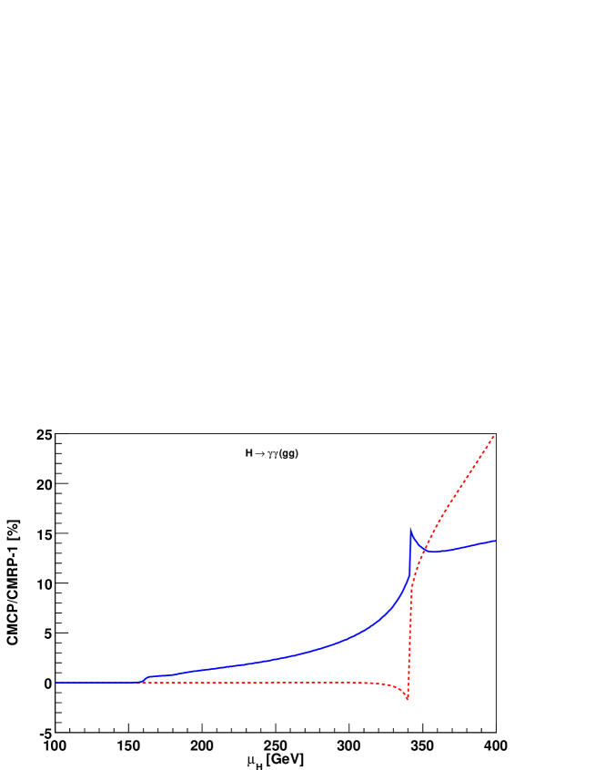
Refer to caption
Figure 10: Comparison of predictions in the CMRP and CMCP schemes for the decays Hγγ𝐻𝛾𝛾H\to\gamma\gamma (blue, solid line) and for Hgg𝐻𝑔𝑔H\to gg (red, dashed line). See Section 8 for the scheme definitions.
Refer to caption
Figure 11: Comparison of the decay width Γ(Hgg)Γ𝐻𝑔𝑔\Gamma(H\to gg) in the CMRP (dashed line) and the CMCP (dotted line) scheme in the high mass region. The effect of a complex top quark pole in CMCP (with a top total, on-shell, width of 13.113.113.1\,GeV) is given by the blue, solid line. See Section 8 for the scheme definitions.
Refer to caption
Figure 12: Comparison of the decay width Γ(Hγγ)Γ𝐻𝛾𝛾\Gamma(H\to\gamma\gamma) in the RMRP (dotted line), the CMRP (dashed line) and the CMCP (solid line) scheme. The effect of a complex top quark pole in CMCP (with a top total, on-shell, width of 13.113.113.1\,GeV) is given by the blue, dash-dotted line. The red, dash-double-dotted line corresponds to a top width of 1.311.311.31\,GeV. See Section 8 for the scheme definitions.

The relatively large effects in Γ(Hγγ)Γ𝐻𝛾𝛾\Gamma(H\to\gamma\gamma) or Γ(Hgg)Γ𝐻𝑔𝑔\Gamma(H\to gg) at large values of μHsubscript𝜇𝐻\mu_{{\scriptscriptstyle{H}}} are still compatible with the naive 𝒪(γH/μH)𝒪subscript𝛾𝐻subscript𝜇𝐻{\cal O}\left(\gamma_{{\scriptscriptstyle{H}}}/\mu_{{\scriptscriptstyle{H}}}\right) argument. Consider Fig. 10 for Γ(Hγγ)Γ𝐻𝛾𝛾\Gamma(H\to\gamma\gamma); for instance, at μH=365subscript𝜇𝐻365\mu_{{\scriptscriptstyle{H}}}=365\,GeV we have γH/μH=0.065subscript𝛾𝐻subscript𝜇𝐻0.065\gamma_{{\scriptscriptstyle{H}}}/\mu_{{\scriptscriptstyle{H}}}=0.065 with a variation between the CMRP and CMCP schemes of 13.3%percent13.313.3\% giving a correction factor of 2γH/μH2subscript𝛾𝐻subscript𝜇𝐻2\,\gamma_{{\scriptscriptstyle{H}}}/\mu_{{\scriptscriptstyle{H}}}. Clearly, the large increase in the Higgs boson width for increasing values of μHsubscript𝜇𝐻\mu_{{\scriptscriptstyle{H}}} makes it questionable to use a perturbative description for the Higgs-resonant part of ppX𝑝𝑝𝑋pp\to X when we have a very heavy Higgs boson.

The relevance of this result is clear: if a light Higgs boson is not discovered, one of the goals of LHC will be to exclude a standard model Higgs up to 600600600\,GeV [37]; already at 500500500\,GeV we have

σCMCP(ggH)σCMRP(ggH)=1.64,parton level,subscript𝜎CMCP𝑔𝑔𝐻subscript𝜎CMRP𝑔𝑔𝐻1.64parton level\frac{\sigma_{\rm{\scriptscriptstyle{CMCP}}}(gg\to H)}{\sigma_{\rm{\scriptscriptstyle{CMRP}}}(gg\to H)}=1.64,\qquad\hbox{parton level}, (141)

comparable to the effect of NLO QCD corrections. We have computed also σ(ppH)𝜎𝑝𝑝𝐻\sigma(pp\to H) in the two schemes using MSTW 2008 LO parton distribution functions (PDF) [34]. The ratio is given in Fig. 13, for different values of s𝑠s; in this figure we present

σCMCP(ppH)σCMRP(ppH),subscript𝜎CMCP𝑝𝑝𝐻subscript𝜎CMRP𝑝𝑝𝐻\frac{\sigma_{\rm{\scriptscriptstyle{CMCP}}}(pp\to H)}{\sigma_{\rm{\scriptscriptstyle{CMRP}}}(pp\to H)}, (142)
Refer to caption
Figure 13: The ratio σCMCP/σCMRPsubscript𝜎CMCPsubscript𝜎CMRP\sigma_{\rm{\scriptscriptstyle{CMCP}}}/\sigma_{\rm{\scriptscriptstyle{CMRP}}} for the production cross section ppH𝑝𝑝𝐻pp\to H, as a function of μHsubscript𝜇𝐻\mu_{{\scriptscriptstyle{H}}}, for different energies, s=3𝑠3\sqrt{s}=3\,TeV (red, dotted line), s=10𝑠10\sqrt{s}=10\,TeV (blue, dashed line) and s=14𝑠14\sqrt{s}=14\,TeV (black, solid line). The cross sections are computed with MSTW2008 LO PDFs with factorization scale μF=μHsubscript𝜇𝐹subscript𝜇𝐻\mu_{{\scriptscriptstyle{F}}}=\mu_{{\scriptscriptstyle{H}}} for CMRP and μF=μ¯Hsubscript𝜇𝐹subscript¯𝜇𝐻\mu_{{\scriptscriptstyle{F}}}={\overline{\mu}}_{{\scriptscriptstyle{H}}} for CMCP.

where the numerator is evaluated at μ¯Hsubscript¯𝜇𝐻{\overline{\mu}}_{{\scriptscriptstyle{H}}} (Eq.(18)) while the denominator corresponds to μHsubscript𝜇𝐻\mu_{{\scriptscriptstyle{H}}}. Here we use

σ(ppH)=σ0τHdLggdτH,dLggdτ=τ1dxxg(x,μF)g(τx,μF),formulae-sequence𝜎𝑝𝑝𝐻subscript𝜎0subscript𝜏𝐻𝑑superscript𝐿𝑔𝑔𝑑subscript𝜏𝐻𝑑superscript𝐿𝑔𝑔𝑑𝜏superscriptsubscript𝜏1𝑑𝑥𝑥𝑔𝑥subscript𝜇𝐹𝑔𝜏𝑥subscript𝜇𝐹\sigma(pp\to H)=\sigma_{0}\,\tau_{{\scriptscriptstyle{H}}}\,\frac{dL^{gg}}{d\tau_{{\scriptscriptstyle{H}}}},\qquad\frac{dL^{gg}}{d\tau}=\int_{\tau}^{1}\,\frac{dx}{x}\,g\left(x,\mu_{{\scriptscriptstyle{F}}}\right)\,g\left(\frac{\tau}{x},\mu_{{\scriptscriptstyle{F}}}\right), (143)

where τ=μH2(μ¯H2)/s𝜏subscriptsuperscript𝜇2𝐻subscriptsuperscript¯𝜇2𝐻𝑠\tau=\mu^{2}_{{\scriptscriptstyle{H}}}({\overline{\mu}}^{2}_{{\scriptscriptstyle{H}}})/s, σ0subscript𝜎0\sigma_{0} is the parton level cross section and g𝑔g is the gluon PDF (with factorization scale μF=μHsubscript𝜇𝐹subscript𝜇𝐻\mu_{{\scriptscriptstyle{F}}}=\mu_{{\scriptscriptstyle{H}}} for CMRP and μF=μ¯Hsubscript𝜇𝐹subscript¯𝜇𝐻\mu_{{\scriptscriptstyle{F}}}={\overline{\mu}}_{{\scriptscriptstyle{H}}} for CMCP).

Note that this ratio is only an indicator of the (large) size of the effect since, for a realistic value of the cross section, NLO(NNLO) QCD corrections should be included, see Ref. [35] for updated cross sections at the Tevatron and the LHC.

In Fig. 14 we show the corresponding cross section for s=3𝑠3\sqrt{s}=3\,TeV, including an estimate of the uncertainty induced by varying renormalization and factorization scales (kept equal for simplicity); μH/2μR=μF2μHsubscript𝜇𝐻2subscript𝜇𝑅subscript𝜇𝐹2subscript𝜇𝐻\mu_{{\scriptscriptstyle{H}}}/2\leq\mu_{{\scriptscriptstyle{R}}}=\mu_{{\scriptscriptstyle{F}}}\leq 2\,\mu_{{\scriptscriptstyle{H}}} for CMRP and μ¯H/2μR=μF2μ¯Hsubscript¯𝜇𝐻2subscript𝜇𝑅subscript𝜇𝐹2subscript¯𝜇𝐻{\overline{\mu}}_{{\scriptscriptstyle{H}}}/2\leq\mu_{{\scriptscriptstyle{R}}}=\mu_{{\scriptscriptstyle{F}}}\leq 2\,{\overline{\mu}}_{{\scriptscriptstyle{H}}} for CMCP (μ¯Hsubscript¯𝜇𝐻{\overline{\mu}}_{{\scriptscriptstyle{H}}} is given in Eq.(18)). In Fig. 14 we do not include the uncertainty associated to PDFs.
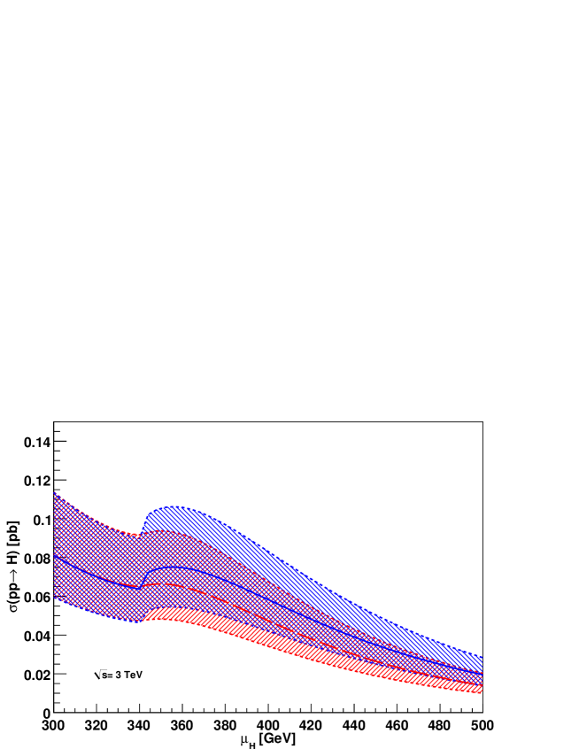
Refer to caption
Figure 14: The production cross section ppH𝑝𝑝𝐻pp\to H at s=3𝑠3\sqrt{s}=3\,TeV for CMRP (red, wide-dashed line) and CMCP (blue, solid line). The shaded areas surrounded by the dashed lines give the scale uncertainty obtained by varying μH/2<μR=μF<2μHsubscript𝜇𝐻2subscript𝜇𝑅subscript𝜇𝐹2subscript𝜇𝐻\mu_{{\scriptscriptstyle{H}}}/2<\mu_{{\scriptscriptstyle{R}}}=\mu_{{\scriptscriptstyle{F}}}<2\,\mu_{{\scriptscriptstyle{H}}} in the CMRP scheme and μ¯H/2<μR=μF<2μ¯Hsubscript¯𝜇𝐻2subscript𝜇𝑅subscript𝜇𝐹2subscript¯𝜇𝐻{\overline{\mu}}_{{\scriptscriptstyle{H}}}/2<\mu_{{\scriptscriptstyle{R}}}=\mu_{{\scriptscriptstyle{F}}}<2\,{\overline{\mu}}_{{\scriptscriptstyle{H}}} (Eq.(18)) in the CMCP scheme. We have used MSTW2008 LO PDFs.

The ratio between the two cross sections is stable under these variations, e.g. is between 1.45461.45461.4546 and 1.45741.45741.4574 at s=10𝑠10\sqrt{s}=10\,TeV and μH=500subscript𝜇𝐻500\mu_{{\scriptscriptstyle{H}}}=500\,GeV. The production cross sections for s=10,14𝑠1014\sqrt{s}=10,14\, TeV are shown in Fig. 15; note that here we use αS(MZ)=0.13934subscript𝛼𝑆subscript𝑀𝑍0.13934\alpha_{{\scriptscriptstyle{S}}}(M_{{\scriptscriptstyle{Z}}})=0.13934 to be consistent with the LO PDFs [34].
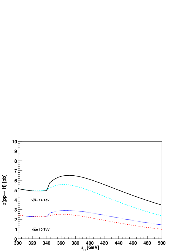
Refer to caption
Figure 15: The production cross section ppH𝑝𝑝𝐻pp\to H at s=10𝑠10\sqrt{s}=10\,TeV for CMRP (red, dashed-dotted line) and CMCP (blue, dotted line); at s=14𝑠14\sqrt{s}=14\,TeV for CMRP (cyan, dashed line) and CMCP (black, solid line). We have used MSTW2008 LO PDFs with factorization scale μF=μHsubscript𝜇𝐹subscript𝜇𝐻\mu_{{\scriptscriptstyle{F}}}=\mu_{{\scriptscriptstyle{H}}} for CMRP and μF=μ¯Hsubscript𝜇𝐹subscript¯𝜇𝐻\mu_{{\scriptscriptstyle{F}}}={\overline{\mu}}_{{\scriptscriptstyle{H}}} for CMCP.

In order to better understand the numerical differences in the three schemes we show in Fig. 16 a scalar two-point function with two internal Z𝑍Z masses.

Refer to caption
Figure 16: The scalar two-point function with two real internal masses (RMRP scheme) MZ2subscriptsuperscript𝑀2𝑍M^{2}_{{\scriptscriptstyle{Z}}} or two complex internal masses (CMRP - CMCP schemes) sZsubscript𝑠𝑍s_{{\scriptscriptstyle{Z}}}. B0subscript𝐵0B_{0} is computed in the RMRP (red dash-line), CMRP (blue dot-line) and CMCP (black solid-line) schemes. The Mandelstam invariant is μH2subscriptsuperscript𝜇2𝐻\mu^{2}_{{\scriptscriptstyle{H}}} in the RMRP - CMRP schemes and sHsubscript𝑠𝐻s_{{\scriptscriptstyle{H}}} in the CMCP scheme, with 100GeV<μH<500GeV100GeVsubscript𝜇𝐻500GeV100\,\mathrm{GeV}<\mu_{{\scriptscriptstyle{H}}}<500\,\mathrm{GeV}. See Section 8 for the scheme definitions.

In the RMRP scheme both the internal masses and the Mandelstam invariant μH2subscriptsuperscript𝜇2𝐻\mu^{2}_{{\scriptscriptstyle{H}}} are real; in the CMRP scheme we replace MZ2subscriptsuperscript𝑀2𝑍M^{2}_{{\scriptscriptstyle{Z}}} with the corresponding complex pole, sZsubscript𝑠𝑍s_{{\scriptscriptstyle{Z}}}; finally, in the CMCP scheme, also the invariant becomes complex and equal to sHsubscript𝑠𝐻s_{{\scriptscriptstyle{H}}}. In Fig. 16 we vary μHsubscript𝜇𝐻\mu_{{\scriptscriptstyle{H}}} between 100100100\,GeV and 500500500\,GeV where γH=146.89subscript𝛾𝐻146.89\gamma_{{\scriptscriptstyle{H}}}=146.89\,GeV is huge; here deviations between CMRP and CMCP become sizable. This simple example shows the general features of one-loop corrections in the three schemes; CMRP - CMCP smoothly interpolate the RMRP results around normal thresholds and, when μH2subscriptsuperscript𝜇2𝐻\mu^{2}_{{\scriptscriptstyle{H}}} becomes larger and larger, CMCP starts deviating from RMRP - CMRP.

We also consider the expression for the amplitude A(Hγγ)𝐴𝐻𝛾𝛾A\left(H\to\gamma\gamma\right) which can be split into a part containing only C0subscript𝐶0C_{0}\,-functions and a rational term. We write

Γ(Hγγ)=α2GF322π3sW2μ¯H|A|2.\Gamma\left(H\to\gamma\gamma\right)=\frac{\alpha^{2}\,G_{{\scriptscriptstyle{F}}}}{32\,\sqrt{2}\,\pi^{3}}\,\frac{\mid s_{{\scriptscriptstyle{W}}}\mid^{2}}{{\overline{\mu}}_{{\scriptscriptstyle{H}}}}\,\Bigr{|}A\Bigr{|}^{2}. (144)

If we introduce auxiliary variables,

μ¯H2=μH(μH2+γH2)1/2,xt=mt2μ¯H2,xH=sHμ¯H2,xW=sWμ¯H2,formulae-sequencesubscriptsuperscript¯𝜇2𝐻subscript𝜇𝐻superscriptsubscriptsuperscript𝜇2𝐻subscriptsuperscript𝛾2𝐻12formulae-sequencesubscript𝑥𝑡subscriptsuperscript𝑚2𝑡subscriptsuperscript¯𝜇2𝐻formulae-sequencesubscript𝑥𝐻subscript𝑠𝐻subscriptsuperscript¯𝜇2𝐻subscript𝑥𝑊subscript𝑠𝑊subscriptsuperscript¯𝜇2𝐻{\overline{\mu}}^{2}_{{\scriptscriptstyle{H}}}=\mu_{{\scriptscriptstyle{H}}}\,\left(\mu^{2}_{{\scriptscriptstyle{H}}}+\gamma^{2}_{{\scriptscriptstyle{H}}}\right)^{1/2},\quad x_{t}=\frac{m^{2}_{t}}{{\overline{\mu}}^{2}_{{\scriptscriptstyle{H}}}},\quad x_{{\scriptscriptstyle{H}}}=\frac{s_{{\scriptscriptstyle{H}}}}{{\overline{\mu}}^{2}_{{\scriptscriptstyle{H}}}},\quad x_{{\scriptscriptstyle{W}}}=\frac{s_{{\scriptscriptstyle{W}}}}{{\overline{\mu}}^{2}_{{\scriptscriptstyle{H}}}}, (145)

the amplitude can be written as A=AC+R𝐴subscript𝐴𝐶𝑅A=A_{{\scriptscriptstyle{C}}}+R where

ACsubscript𝐴𝐶\displaystyle A_{{\scriptscriptstyle{C}}} =\displaystyle= 83xtxH4xtxWC0(0, 0,sH,mt,mt,mt)+6(xH2xW)C0(0, 0,sH,sW,sW,sW),83subscript𝑥𝑡subscript𝑥𝐻4subscript𝑥𝑡subscript𝑥𝑊subscript𝐶00 0subscript𝑠𝐻subscript𝑚𝑡subscript𝑚𝑡subscript𝑚𝑡6subscript𝑥𝐻2subscript𝑥𝑊subscript𝐶00 0subscript𝑠𝐻subscript𝑠𝑊subscript𝑠𝑊subscript𝑠𝑊\displaystyle-\,\frac{8}{3}\,x_{t}\,\frac{x_{{\scriptscriptstyle{H}}}-4\,x_{t}}{x_{{\scriptscriptstyle{W}}}}\,C_{0}\left(0\,,\,0\,,\,-s_{{\scriptscriptstyle{H}}}\,,\,m_{t}\,,\,m_{t}\,,\,m_{t}\right)+6\,\left(x_{{\scriptscriptstyle{H}}}-2\,x_{{\scriptscriptstyle{W}}}\right)\,C_{0}\left(0\,,\,0\,,\,-s_{{\scriptscriptstyle{H}}}\,,\,s_{{\scriptscriptstyle{W}}}\,,\,s_{{\scriptscriptstyle{W}}}\,,\,s_{{\scriptscriptstyle{W}}}\right),
R𝑅\displaystyle R =\displaystyle= 163xtxW+xHxW+6.163subscript𝑥𝑡subscript𝑥𝑊subscript𝑥𝐻subscript𝑥𝑊6\displaystyle-\,\frac{16}{3}\,\frac{x_{t}}{x_{{\scriptscriptstyle{W}}}}+\frac{x_{{\scriptscriptstyle{H}}}}{x_{{\scriptscriptstyle{W}}}}+6. (146)

A comparison for the real and imaginary parts in the CMRP and CMCP schemes is shown in Fig. 17.
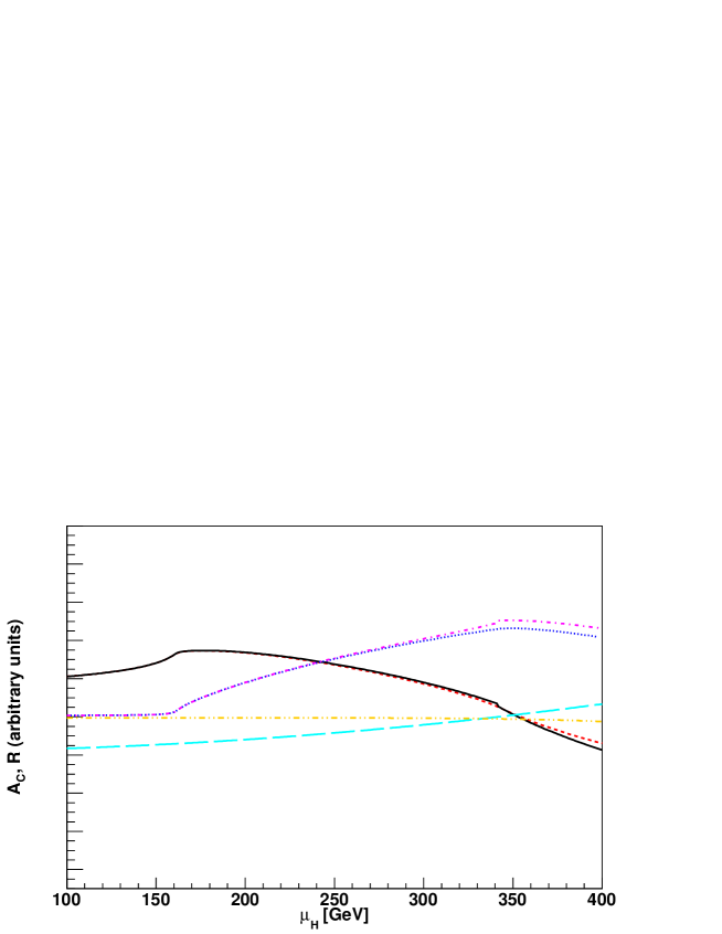
Refer to caption
Figure 17: The C0subscript𝐶0C_{0} part of the amplitude for Hγγ𝐻𝛾𝛾H\to\gamma\gamma and the corresponding rational term of Eq.(146) with 100GeV<μH<300GeV100GeVsubscript𝜇𝐻300GeV100\,\mathrm{GeV}<\mu_{{\scriptscriptstyle{H}}}<300\,\mathrm{GeV}. The black, solid (CMCP) and red, dashed (CMRP) lines give the real part whereas blue, dotted (CMRP) and magenta, dash-dotted (CMCP) lines give the imaginary part. The cyan, wide-dashed (orange, dash-double-dotted) line gives the rational real(imaginary) part of the amplitude without appreciable differences between the schemes. The imaginary part of the rational term is always small and negligible. See Section 8 for the scheme definitions.
  • 𝐇𝐛¯𝐛𝐇¯𝐛𝐛\mathbf{H\to\overline{b}b}

Results for Hb¯b𝐻¯𝑏𝑏H\to\overline{b}b are shown in Tab. 3 for the pure weak percentage one-loop corrections in the three schemes and for a wide range of Higgs masses;

MHsubscript𝑀𝐻M_{{}_{H}}\;[GeV] δWsubscript𝛿𝑊\delta_{{\scriptscriptstyle{W}}} RMRP [%percent\%] δWsubscript𝛿𝑊\delta_{{\scriptscriptstyle{W}}} CMRP [%percent\%] δWsubscript𝛿𝑊\delta_{{\scriptscriptstyle{W}}} CMCP [%percent\%] δWsubscript𝛿𝑊\delta_{{\scriptscriptstyle{W}}} CMCP [%percent\%]
massless massless massless massive
120120120 0.78900.7890-0.7890 0.79040.7904-0.7904 0.79040.7904-0.7904 0.78370.7837-0.7837
130130130 0.95570.9557-0.9557 0.95720.9572-0.9572 0.95730.9573-0.9573 0.95090.9509-0.9509
140140140 1.19781.1978-1.1978 1.19861.1986-1.1986 1.19861.1986-1.1986 1.19221.1922-1.1922
150150150 1.62151.6215-1.6215 1.61461.6146-1.6146 1.61491.6149-1.6149 1.60781.6078-1.6078
160160160 4.26564.2656-4.2656 2.64582.6458-2.6458 2.66902.6690-2.6690 2.65872.6587-2.6587
170170170 1.39871.3987-1.3987 1.49141.4914-1.4914 1.48751.4875-1.4875 1.48221.4822-1.4822
180180180 2.19892.1989-2.1989 1.94351.9435-1.9435 1.99121.9912-1.9912 1.98581.9858-1.9858
190190190 1.03381.0338-1.0338 1.17441.1744-1.1744 1.15901.1590-1.1590 1.15691.1569-1.1569
200200200 1.15471.1547-1.1547 1.19671.1967-1.1967 1.19871.1987-1.1987 1.19741.1974-1.1974
210210210 1.24521.2452-1.2452 1.26211.2621-1.2621 1.27301.2730-1.2730 1.27231.2723-1.2723
220220220 1.31321.3132-1.3132 1.31981.3198-1.3198 1.33791.3379-1.3379 1.33761.3376-1.3376
230230230 1.36471.3647-1.3647 1.36651.3665-1.3665 1.39141.3914-1.3914 1.39171.3917-1.3917
240240240 1.40471.4047-1.4047 1.40441.4044-1.4044 1.43631.4363-1.4363 1.43701.4370-1.4370
250250250 1.43761.4376-1.4376 1.43651.4365-1.4365 1.47591.4759-1.4759 1.47691.4769-1.4769
260260260 1.46741.4674-1.4674 1.46651.4665-1.4665 1.51381.5138-1.5138 1.51511.5151-1.5151
270270270 1.49851.4985-1.4985 1.49811.4981-1.4981 1.55391.5539-1.5539 1.55551.5555-1.5555
280280280 1.53571.5357-1.5357 1.53611.5361-1.5361 1.60081.6008-1.6008 1.60261.6026-1.6026
290290290 1.58511.5851-1.5851 1.58651.5865-1.5865 1.66041.6604-1.6604 1.66241.6624-1.6624
300300300 1.65571.6557-1.6557 1.65821.6582-1.6582 1.74101.7410-1.7410 1.74311.7431-1.7431
400400400 0.47360.4736-0.4736 0.48650.4865-0.4865 0.85890.8589-0.8589 0.86330.8633-0.8633
450450450 +1.48551.4855+1.4855 +1.46871.4687+1.4687 +1.15791.1579+1.1579 +1.15171.1517+1.1517
Table 3: Percentage one-loop pure weak corrections for Hb¯b𝐻¯𝑏𝑏H\to\overline{b}b; the first entry is the RMRP scheme, the second entry is the CMRP scheme, the third entry is the CMCP scheme while the fourth entry is the CMCP scheme with finite mbsubscript𝑚𝑏m_{b} (Section 8).

in Tab. 4 the electroweak (weak + QED) percentage one-loop corrections are given.

MHsubscript𝑀𝐻M_{{}_{H}}\;[GeV] δEWsubscript𝛿EW\delta_{\rm{\scriptscriptstyle{EW}}} CMRP [%percent\%] δEWsubscript𝛿EW\delta_{\rm{\scriptscriptstyle{EW}}} CMCP [%percent\%]
120120120 0.97280.9728-0.9728 0.97290.9729-0.9729
130130130 1.14671.1467-1.1467 1.14681.1468-1.1468
140140140 1.39411.3941-1.3941 1.39421.3942-1.3942
150150150 1.81511.8151-1.8151 1.81541.8154-1.8154
160160160 2.84852.8485-2.8485 2.87162.8716-2.8716
170170170 1.70391.7039-1.7039 1.70001.7000-1.7000
180180180 2.16062.1606-2.1606 2.20832.2083-2.2083
190190190 1.39901.3990-1.3990 1.38371.3837-1.3837
200200200 1.42621.4262-1.4262 1.42831.4283-1.4283
210210210 1.49611.4961-1.4961 1.50711.5071-1.5071
220220220 1.55801.5580-1.5580 1.57611.5761-1.5761
230230230 1.60871.6087-1.6087 1.63371.6337-1.6337
240240240 1.65031.6503-1.6503 1.68241.6824-1.6824
250250250 1.68611.6861-1.6861 1.72561.7256-1.7256
260260260 1.71941.7194-1.7194 1.76691.7669-1.7669
270270270 1.75431.7543-1.7543 1.81021.8102-1.8102
280280280 1.79531.7953-1.7953 1.86021.8602-1.8602
290290290 1.84871.8487-1.8487 1.92281.9228-1.9228
300300300 1.92321.9232-1.9232 2.00612.0061-2.0061
400400400 0.77540.7754-0.7754 1.14881.1488-1.1488
450450450 +1.16971.1697+1.1697 +0.85710.8571+0.8571
Table 4: Percentage one-loop electroweak (weak + QED) corrections for Hb¯b𝐻¯𝑏𝑏H\to\overline{b}b with a massive b-quark; the first entry is the CMRP scheme, the second entry is the CMCP scheme (Section 8).

For weak corrections the results for Hb¯b𝐻¯𝑏𝑏H\to\overline{b}b are presented graphically in Fig. 18;

Refer to caption
Figure 18: The weak one-loop radiative corrections to Hb¯b𝐻¯𝑏𝑏H\to\overline{b}b in the RMRP scheme (red, dotted line), in the CMRP scheme (black, dashed line) and in the CMCP scheme (black, solid line). The effect of a complex top quark pole in CMCP (with a top total, on-shell, width of 13.113.113.1\,GeV) is given by the blue wide-dashed line. See Section 8 for the scheme definitions. The result corresponding to Γt=ΓtNLO=1.31subscriptΓ𝑡subscriptsuperscriptΓNLO𝑡1.31\Gamma_{t}=\Gamma^{\rm{\scriptscriptstyle{NLO}}}_{t}=1.31\,GeV has no appreciable difference compared to the one at Γt=0subscriptΓ𝑡0\Gamma_{t}=0.

the figure shows cusps at the t¯t¯𝑡𝑡\overline{t}t\,-threshold due to the fact that the top quark mass is kept real. The origin of the cusps is in a B0subscript𝐵0B_{0}\,-function with p2superscript𝑝2p^{2} fixed at the complex Higgs pole. The size of the cusps can be related to the large Higgs width at the t¯t¯𝑡𝑡\overline{t}t\,-threshold as illustrated in Fig. 19 where we analyze ReB0(sH;mt,mt)Resubscript𝐵0subscript𝑠𝐻subscript𝑚𝑡subscript𝑚𝑡{\rm{Re}}\,B_{0}(-s_{{\scriptscriptstyle{H}}}\,;\,m_{t},m_{t}) around the t¯t¯𝑡𝑡\overline{t}t threshold. Here the solid line corresponds to γH=0subscript𝛾𝐻0\gamma_{{\scriptscriptstyle{H}}}=0, whereas dash-lines correspond to increasing values of γHsubscript𝛾𝐻\gamma_{{\scriptscriptstyle{H}}}. As one can see the limit γH0subscript𝛾𝐻0\gamma_{{\scriptscriptstyle{H}}}\to 0 is continuous and there is no artifact due to the analytical continuation. The wide-dashed blue line of Fig. 19 corresponds to a finite value of γHsubscript𝛾𝐻\gamma_{{\scriptscriptstyle{H}}} and to a complex top pole (with an on-shell width of 13.113.113.1\,GeV).

Refer to caption
Figure 19: The ReB0(sH;mt,mt)Resubscript𝐵0subscript𝑠𝐻subscript𝑚𝑡subscript𝑚𝑡{\rm{Re}}\,B_{0}(-s_{{\scriptscriptstyle{H}}}\,;\,m_{t},m_{t}) around the t¯t¯𝑡𝑡\overline{t}t threshold. The solid line corresponds to a real Higgs mass, γH=0subscript𝛾𝐻0\gamma_{{\scriptscriptstyle{H}}}=0, whereas dashed lines correspond to increasing values of γHsubscript𝛾𝐻\gamma_{{\scriptscriptstyle{H}}}. The blue, wide-dashed line corresponds to a finite γHsubscript𝛾𝐻\gamma_{{\scriptscriptstyle{H}}} and to a complex top quark pole (with an on-shell width of 13.113.113.1\,GeV).

As it is evident the introduction of a complex top quark pole completely cures the shape of the corrections. Therefore, this gives further evidence to using the CMCP scheme, at least from a theoretical point of view (the top quark total width is, unfortunately, poorly known). It is worth noting that the numerical effect given by the blue curve should be interpreted as an upper bound on the effect of a top quark complex pole since the experimental result is an upper bound, Γt<13.1subscriptΓ𝑡13.1\Gamma_{t}<13.1\,GeV at 95%percent9595\% C.L. Note that, from theory it follows ΓtLO=1.47subscriptsuperscriptΓLO𝑡1.47\Gamma^{\rm{\scriptscriptstyle{LO}}}_{t}=1.47\,GeV and ΓtNLO=1.31subscriptsuperscriptΓNLO𝑡1.31\Gamma^{\rm{\scriptscriptstyle{NLO}}}_{t}=1.31\,GeV.

Finally, we observe that the 𝒪(γH/μH)𝒪subscript𝛾𝐻subscript𝜇𝐻{\cal O}\left(\gamma_{{\scriptscriptstyle{H}}}/\mu_{{\scriptscriptstyle{H}}}\right) effects, which can reach several percent at large values of μHsubscript𝜇𝐻\mu_{{\scriptscriptstyle{H}}}, have a modest effect on all those processes which start at 𝒪(g2)𝒪superscript𝑔2{\cal O}\left(g^{2}\right) (the effect being on NLO corrections) whereas the effect is considerably larger for those processes, e.g. Hγγ(gg)𝐻𝛾𝛾𝑔𝑔H\to\gamma\gamma(gg), which start directly at NLO (𝒪(g6)𝒪superscript𝑔6{\cal O}\left(g^{6}\right)).

10 Conclusions

In this paper we have shown how to continue Feynman integrals into the second Riemann sheet, in a way that can be easily implemented in any program aimed to compute pseudo-observables related to Higgs physics at Tevatron and LHC. Pseudo-observables give, in a natural way, the possibility of translating experimental data into a language that has a direct connection to unambiguous theoretical calculations. Using our framework one can freely compute quantities (otherwise non-existing) like Higgs production cross section and Higgs partial decay widths.

An unstable particle cannot belong to the in/out basis of the Hilbert space, nevertheless concepts like production or decay of an unstable particle becomes aliases for pseudo-observables that have a well defined meaning and a direct relation to measured data.

In this paper a new scheme is introduced which is the (complete) complex mass scheme with complex, external Higgs boson (or, equivalently, any other external unstable particle) where the LSZ procedure is carried out at the Higgs complex pole (on the second Riemann sheet).

Pseudo-observables have been a very useful concept at LEP (e.g. Ref.[36]) and will continue to play an important role at LHC, although more difficult if deviations from the SM will emerge; in this case model independent approaches are required allowing for the extraction of useful quantities that can be fitted with different models.

The usual objection against moving standard model Higgs pseudo-observables into the second Riemann sheet of the S𝑆S\,-matrix is that a light Higgs boson, say below 140140140\,GeV, has a very narrow width and the effects induced are tiny. Admittedly, it is a well taken point for all practical consequences but one should remember that the Higgs boson width rapidly increases after the opening of the WW𝑊𝑊WW and ZZ𝑍𝑍ZZ channels and, because of this, the on-shell treatment of an external Higgs particle becomes inadequate as a description of data if the Higgs is not (very) light.

Furthermore, most of the experimental plots concerning Higgs physics extend well above, say, 200200200\,GeV and, if a light Higgs boson is not discovered, one of the goals of LHC will be to exclude a standard model Higgs up to 600600600\,GeV (see Ref. [37] for an exclusion plot of the SM Higgs boson for the various channels as well as the combination for masses up to 600600600\,GeV). Already at 500500500\,GeV the ratio CMCP/CMRP for the ggH𝑔𝑔𝐻gg\to H cross section is large and comparable to higher order QCD corrections.

On top of all practical implications one should admit that it is hard to sustain a wrong theoretical description of experimental data if the correct one is available, independently on the size of the effect.

Finally, our results show that, above the t¯t¯𝑡𝑡\overline{t}t\,-threshold the Higgs-resonant contribution to ppX𝑝𝑝𝑋pp\to X, correctly described in the CMCP scheme, is strongly influenced by the large imaginary part of the Higgs complex pole and the use of the conventional on-shell description of Higgs pseudo-observables becomes highly questionable, even from a numerical point of view.


Acknowledgments

G.P. is indebted to Stefan Dittmaier for an important discussion on H4𝐻4H\to 4\,f. We gratefully acknowledge several discussions with W. Hollik and R. Pittau.

References

  • [1] T. N. Phenomena, H. w. group, f. t. C. collaboration and D. collaboration, arXiv:0903.4001 [hep-ex];
    T. C. Collaboration, t. D. Collaboration, t. T. N. Physics and H. W. Group, arXiv:0911.3930 [hep-ex].
  • [2] J. Fernandez, f. t. ATLAS and C. Collaborations, arXiv:0905.1228 [hep-ex].
  • [3] C. Anastasiou, R. Boughezal and F. Petriello, JHEP 0904, 003 (2009) [arXiv:0811.3458 [hep-ph]];
    C. Anastasiou, AIP Conf. Proc.  806, 75 (2006);
    C. Anastasiou, K. Melnikov and F. Petriello, Phys. Rev.  D 72, 097302 (2005) [arXiv:hep-ph/0509014];
    C. Anastasiou, K. Melnikov and F. Petriello, Phys. Rev. Lett.  93, 262002 (2004) [arXiv:hep-ph/0409088];
    C. Anastasiou and K. Melnikov, Nucl. Phys.  B 646, 220 (2002) [arXiv:hep-ph/0207004];
    R. Boughezal, arXiv:0908.3969 [hep-ph].
  • [4] M. Grazzini, Nucl. Phys. Proc. Suppl.  183, 25 (2008);
    D. de Florian and M. Grazzini, arXiv:0901.2427 [hep-ph];
    M. Grazzini, arXiv:0806.3336 [hep-ph].
  • [5] S. Actis, G. Passarino, C. Sturm and S. Uccirati, Phys. Lett.  B 669 (2008) 62 [arXiv:0809.1302 [hep-ph]];
    S. Actis, G. Passarino, C. Sturm and S. Uccirati, Nucl. Phys.  B 811 (2009) 182 [arXiv:0809.3667 [hep-ph]];
    G. Passarino, C. Sturm and S. Uccirati, Phys. Lett.  B 655 (2007) 298 [arXiv:0707.1401 [hep-ph]].
  • [6] R. V. Harlander, H. Mantler, S. Marzani and K. J. Ozeren, arXiv:0912.2104 [hep-ph];
    R. V. Harlander and K. J. Ozeren, JHEP 0911 (2009) 088 [arXiv:0909.3420 [hep-ph]];
    R. V. Harlander and K. J. Ozeren, Phys. Lett.  B 679 (2009) 467 [arXiv:0907.2997 [hep-ph]];
    A. Pak, M. Rogal and M. Steinhauser, arXiv:0911.4662 [hep-ph];
    A. Pak, M. Rogal and M. Steinhauser, Phys. Lett.  B 679, 473 (2009) [arXiv:0907.2998 [hep-ph]].
  • [7] R. E. Cutkosky, J. Math. Phys.  1 (1960) 429.
  • [8] M. J. G. Veltman, Physica 29, 186 (1963).
  • [9] C. Mœller, K. Danske. Vid. Selsk. 22, no 19 (1946);
    R. Peierls, Proceedings of the 1954 Glasgow Conference on Nuclear and Meson Physics, (Pergamon Press, New York, 1955) p. 296;
    R. Jacob and R. G. Sachs, Phys. Rev.  121 (1961) 350.
  • [10] P. A. Grassi, B. A. Kniehl and A. Sirlin, Phys. Rev. Lett.  86 (2001) 389 [arXiv:hep-th/0005149];
    B. A. Kniehl and A. Sirlin, Phys. Rev. Lett.  81 (1998) 1373 [arXiv:hep-ph/9805390];
    B. A. Kniehl and A. Sirlin, Phys. Rev.  D 77, 116012 (2008) [arXiv:0801.0669 [hep-th]];
    B. A. Kniehl and A. Sirlin, Phys. Lett.  B 530, 129 (2002) [arXiv:hep-ph/0110296].
  • [11] M. Beneke, A. P. Chapovsky, A. Signer and G. Zanderighi, Phys. Rev. Lett.  93 (2004) 011602 [arXiv:hep-ph/0312331].
  • [12] G. Valent, Nucl. Phys.  B 65 (1973) 445;
    J. Lukierski, Fortsch. Phys.  28 (1980) 259;
    C. G. Bollini and L. E. Oxman, Int. J. Mod. Phys.  A 8 (1993) 3185;
    C. G. Bollini and L. E. Oxman, Int. J. Mod. Phys.  A 7 (1992) 6845;
  • [13] R. S. Willey, Phys. Rev.  D 59 (1999) 013009 [Erratum-ibid.  D 61 (2000) 079902] [arXiv:hep-ph/9804392].
  • [14] D. Y. Bardin, M. Grunewald and G. Passarino, arXiv:hep-ph/9902452.
  • [15] R. G. Stuart, Phys. Lett. B 262 (1991) 113;
    A. Sirlin, Phys. Rev. Lett.  67 (1991) 2127;
    E. N. Argyres et al., Phys. Lett. B 358, 339 (1995) [arXiv:hep-ph/9507216];
    W. Beenakker et al., Nucl. Phys. B 500, 255 (1997) [arXiv:hep-ph/9612260];
    G. Passarino, Nucl. Phys.  B 574 (2000) 451 [arXiv:hep-ph/9911482];
    G. Passarino, Nucl. Phys.  B 578 (2000) 3 [arXiv:hep-ph/0001212];
    T. Bhattacharya and S. Willenbrock, Phys. Rev.  D 47 (1993) 4022.
  • [16] P. A. Grassi, B. A. Kniehl and A. Sirlin, Phys. Rev.  D 65, 085001 (2002) [arXiv:hep-ph/0109228];
    P. Gambino and P. A. Grassi, Phys. Rev.  D 62, 076002 (2000) [arXiv:hep-ph/9907254].
  • [17] S. Actis and G. Passarino, Nucl. Phys.  B 777, 100 (2007) [arXiv:hep-ph/0612124].
  • [18] A. Denner, S. Dittmaier, M. Roth and L. H. Wieders, Nucl. Phys. B 724 (2005) 247 [arXiv:hep-ph/0505042];
    A. Denner and S. Dittmaier, Nucl. Phys. Proc. Suppl.  160 (2006) 22 [arXiv:hep-ph/0605312];
    A. Denner, S. Dittmaier, M. Roth and D. Wackeroth, Nucl. Phys. B 560 (1999) 33 [arXiv:hep-ph/9904472].
  • [19] A. Ghinculov and T. Binoth, Phys. Lett.  B 394 (1997) 139 [arXiv:hep-ph/9611357];
    S. Willenbrock and G. Valencia, Phys. Lett.  B 247 (1990) 341.
  • [20] T. Aaltonen et al. [CDF Collaboration], Phys. Rev. Lett.  102 (2009) 042001 [arXiv:0808.2167 [hep-ex]].
  • [21] H. A. Weldon, Phys. Rev.  D 14 (1976) 2030.
  • [22] A. Bredenstein, A. Denner, S. Dittmaier and M. M. Weber, Phys. Rev.  D 74 (2006) 013004 [arXiv:hep-ph/0604011];
    A. Bredenstein, A. Denner, S. Dittmaier and M. M. Weber, JHEP 0702 (2007) 080 [arXiv:hep-ph/0611234];
    C. Buttar et al., arXiv:hep-ph/0604120.
  • [23] H. J. Bremermann and J. L. Durand J. Math. Phys.  2 (1960) 240.
  • [24] L. S. Brown, Cambridge, UK: Univ. Pr. (1992) 542 p.
  • [25] R. Erdelyi et al., Higher Transcendental Functions vol. 1, Bateman Manuscript Project (McGraw-Hill 1953).
  • [26] K. S. Kolbig, SIAM J. Math. Anal.  17 (1986) 1232. N. Nielsen, Nova Acta Leopoldina (Halle) 90 (1909) 123;
    L. Lewin, Polylogarithms and associated functions, North Holland, Amsterdam, 1981.
  • [27] A. Ferroglia, M. Passera, G. Passarino and S. Uccirati, Nucl. Phys.  B 650 (2003) 162 [arXiv:hep-ph/0209219].
  • [28] Z. Nagy and D. E. Soper, Phys. Rev.  D 74 (2006) 093006 [arXiv:hep-ph/0610028].
  • [29] G. ’t Hooft and M. J. G. Veltman, Nucl. Phys.  B 153 (1979) 365.
  • [30] G. Passarino, Nucl. Phys. B 619 (2001) 257 [arXiv:hep-ph/0108252];
    G. Passarino and S. Uccirati, Nucl. Phys. B 629 (2002) 97 [arXiv:hep-ph/0112004];
    J. Bernstein, Modules over a ring of differential operators, Functional Analysis and its Applications 5(1971);
    M. Sato, Nagoya Mat. J. 120 (1990) 1;
    S. C. Coutinho, A Primer of Algebraic D𝐷D-Modules, LMS Student Text 33 (1995);
    F. V. Tkachov, Nucl. Instrum. Meth. A 389 (1997) 309 [hep-ph/9609429].
  • [31] S. Uccirati, Acta Phys. Polon.  B 35 (2004) 2573 [arXiv:hep-ph/0410332].
  • [32] G. Passarino and S. Uccirati, Nucl. Phys.  B 747 (2006) 113 [arXiv:hep-ph/0603121].
  • [33] V. S. Fadin, V. A. Khoze and A. D. Martin, Phys. Lett.  B 320 (1994) 141 [arXiv:hep-ph/9309234].
  • [34] A. D. Martin, W. J. Stirling, R. S. Thorne and G. Watt, Eur. Phys. J.  C 63 (2009) 189 [arXiv:0901.0002 [hep-ph]];
    A. D. Martin, W. J. Stirling, R. S. Thorne and G. Watt, Eur. Phys. J.  C 64 (2009) 653 [arXiv:0905.3531 [hep-ph]].
  • [35] D. de Florian and M. Grazzini, Phys. Lett.  B 674 (2009) 291 [arXiv:0901.2427 [hep-ph]].
  • [36] M. W. Grunewald et al., arXiv:hep-ph/0005309; D. Y. Bardin, M. Grunewald and G. Passarino, arXiv:hep-ph/9902452.
  • [37] ATLAS Collaboration, Expected Performance of the ATLAS Experiment, Detector, Trigger and Physics,CERN-OPEN-2008-020, Geneva, 2008;
    G. L. Bayatian et al. [CMS Collaboration], J. Phys. G 34 (2007) 995.