A Milstein-type scheme without Lévy area terms for SDEs driven by fractional Brownian motion

Abstract.

In this article, we study the numerical approximation of stochastic differential equations driven by a multidimensional fractional Brownian motion (fBm) with Hurst parameter greater than $1/3$. We introduce an implementable scheme for these equations, which is based on a second order Taylor expansion, where the usual Lévy area terms are replaced by products of increments of the driving fBm. The convergence of our scheme is shown by means of a combination of rough paths techniques and error bounds for the discretisation of the Lévy area terms.

1. Introduction and Main Results

Fractional Brownian motion (fBm in short for the remainder of the article) is a natural generalisation of the usual Brownian motion, insofar as it is defined as a centered Gaussian process $B=\{B_{t};\,t\in\mathbb{R}_{+}\}$ with continuous sample paths, whose increments $(\delta B)_{st}:=B_{t}-B_{s}$, $s,t\in\mathbb{R}_{+}$ are characterised by their variance $\mathbf{E}[(\delta B)_{st}^{2}]=|t-s|^{2H}$. Here the parameter $H\in(0,1)$, which is called Hurst parameter, governs in particular the Hölder regularity of the sample paths of $B$ by a standard application of Kolmogorov’s criterion: fBm has Hölder continuous sample paths of order $\lambda$ for all $\lambda<H$. The particular case $H=1/2$ corresponds to the usual Brownian motion, so the cases $H\neq 1/2$ are a natural extension of the classical situation, allowing e.g. any prescribed Hölder regularity of the driving process. Moreover, fBm is $H$-self similar, i.e. for any $c>0$ the process $\{c^{H}B_{t/c};\,t\in\mathbb{R}_{+}\}$ is again a fBm, and also has stationarity increments, that is for any $h\geq 0$ the process $\{B_{t+h}-B_{h};\,t\in\mathbb{R}_{+}\}$ is a fBm.

These properties (partially) explain why stochastic equations driven by fBm have received considerable attention during the last two decades. Indeed, many physical systems seem to be governed by a Gaussian noise with different properties than classical Brownian motion. Fractional Brownian motion as driving noise is used e.g. in electrical engineering [12, 13], or biophysics [5, 23, 34]. Moreover, after some controversial discussions (see [3] for a summary of the early developments) fBm has established itself also in financial modelling, see e.g. [17, 2]. For empirical studies of fractional Brownian motion in finance see e.g. [8, 39, 7]. All these situations lead to different kind of stochastic differential equations (SDEs), whose simplest prototype can be formally written as

$$Y_{t}=a+\sum_{i=1}^{m}\int_{0}^{t}\sigma^{(i)}(Y_{u})\,dB_{u}^{(i)},\quad t\in\left[0,T\right],\qquad a\in\mathbb{R}^{d},$$ (1)

where $\sigma=(\sigma^{(1)},\ldots,\sigma^{(m)})$ is a smooth enough function from $\mathbb{R}^{d}$ to $\mathbb{R}^{d\times m}$ and $B=(B^{(1)},\ldots,B^{(m)})$ is a $m$-dimensional fBm with Hurst parameter $H>1/3$.

At a mathematical level, fractional differential equations of type (1) are typically handled (for $H\neq 1/2$) by pathwise or semi-pathwise methods. Indeed for $H>1/2$, the integrals $\int_{0}^{t}\sigma^{(i)}(Y_{u})\,dB_{u}^{(i)}$, $i=1,\ldots,m,$ in (1) can be defined using Young integration or fractional calculus tools, and these methods also yield the existence of a unique solution, see e.g. [33, 40]. When $1/4<H<1/2$, the existence and uniqueness result for equation (1) can be seen as the canonical example of an application of the rough paths theory. The reader is referred to [16, 25] for the original version of the rough paths theory, and to [18] for a (slightly) simpler algebraic setting which will be used in the current article. In the particular case $1/3<H<1/2$, the rough path machinery can be summarised very briefly as follows: assume that our driving signal $B$ allows to define iterated integrals with respect to itself. Then one can define and solve equation (1) in a reasonable class of processes.

Once SDEs driven by fBm are solved, it is quite natural (as in the case of SDEs driven by the usual Brownian motion) to study the stochastic processes they define. However, even if some progress has been made in this direction, e.g. concerning the law of the solution [1, 4, 29] or its ergodic properties [20], the picture here is far from being complete. Moreover, explicit solutions of stochastic differential equations driven by fBm are rarely known, as in the case of SDEs driven by classical Brownian motion. Thus one has to rely on numerical methods for the simulation of these equations.

So far, some numerical schemes for equations like (1) have already been studied in the literature. In the following, we consider uniform grids of the form $\{t_{k}=kT/n;\,0\leq k\leq n\}$ for a fixed $T>0$. The simplest approximation method is the Euler scheme defined by

$$Y^{n}_{0} =a,$$

$${Y}_{t_{k+1}}^{n} ={Y}_{t_{k}}^{n}+\sum_{i=1}^{m}\sigma^{(i)}({Y}_{t_{k}}^{n})\delta B^{(i)}_{t_{k}t_{k+1}},\qquad k=0,\ldots,n-1.$$

For $H>1/2$, the Euler scheme converges to the solution of the SDE (1). See e.g. in [26], where an almost sure convergence rate $n^{-(2H-1)+\varepsilon}$ with $\varepsilon>0$ arbitrarily small is established. A detailed analysis of the one-dimensional case is given in [28], where the exact convergence rate $n^{-2H+1}$ and the asymptotic error distribution are derived.

However, the Euler scheme is not appropriate to approximate SDEs driven by fBm when $1/3<H<1/2$. This is easily illustrated by the following one-dimensional example, in which $B$ denotes a one-dimensional fBm: consider the equation

$$dY_{t}=Y_{t}\,dB_{t},\quad t\in[0,1],\qquad Y_{0}=1,$$

whose exact solution is

$$Y_{t}=\exp(B_{t}),\quad t\in[0,1].$$

The Euler approximation for this equation at the final time point $t=1$ can be written as

$$Y^{n}_{1}=\prod_{k=0}^{n-1}(1+(\delta B)_{k/n,(k+1)/n}).$$

So for $n\in\mathbb{N}$ sufficiently large and using a Taylor expansion, we have

$$Y^{n}_{1}=\exp\Big{(}\sum_{k=0}^{n-1}\log(1+(\delta B)_{k/n,(k+1)/n})\Big{)}=\exp\Big{(}B_{1}-\frac{1}{2}\sum_{k=0}^{n-1}|(\delta B)_{k/n,(k+1)/n}|^{2}+\rho_{n}\Big{)},$$

where $\lim_{n\rightarrow\infty}\rho_{n}\stackrel{{\scriptstyle\rm a.s.}}{{=}}0$ for $H>1/3$. Now it is well known that

$$\sum_{k=0}^{n-1}|(\delta B)_{k/n,(k+1)/n}|^{2}\stackrel{{\scriptstyle\rm a.s.}}{{\longrightarrow}}\infty$$

for $H<1/2$ as $n\to\infty$, which implies that $\lim_{n\rightarrow\infty}Y^{n}_{1}\stackrel{{\scriptstyle{\rm a.s.}}}{{=}}0$. This is obviously incompatible with a convergence towards $Y_{1}=\exp(B_{1})$. In the case $H=1/2$ this phenomenon is also well known: here the Euler scheme converges to the Itô solution and not to the Stratonovich solution of SDE (1).

To obtain a convergent numerical method Davie proposed in [9] a scheme of Milstein type. For this, assume that all iterated integrals of $B$ with respect to itself are collected into a $m\times m$ matrix $\mathbf{B}^{\mathbf{2}}$, i.e. set

$$\mathbf{B}^{\mathbf{2}}_{st}(i,j)=\int_{s}^{t}\int_{s}^{u}dB_{v}^{(i)}\,dB_{u}^{(j)},\qquad 0\leq s<t\leq T,\quad 1\leq i,j\leq m.$$

The matrix $\mathbf{B}^{\mathbf{2}}$ (respectively its elements) is (are) usually called Lévy area. Davie’s scheme is then given by

$$Y^{n}_{0} =a,$$ (2)

$${Y}_{t_{k+1}}^{n} ={Y}_{t_{k}}^{n}+\sum_{i=1}^{m}\sigma^{(i)}({Y}_{t_{k}}^{n})\delta B^{(i)}_{t_{k}t_{k+1}}+\sum_{i,j=1}^{m}\mathcal{D}^{(i)}\sigma^{(j)}(Y_{t_{k}}^{n})\,\mathbf{B}^{\mathbf{2}}_{t_{k}t_{k+1}}(i,j),\qquad k=0,\ldots,n-1,$$

with the differential operator $\mathcal{D}^{(i)}=\sum_{l=1}^{d}\sigma_{l}^{(i)}\partial_{x_{l}}$. (Recall that we use the notation $\delta B^{(i)}_{st}=B^{(i)}_{t}-B^{(i)}_{s}$ for $s,t\in\left[0,T\right]$.) This scheme is shown to be convergent as long as $H>1/3$ in [9], with an almost sure convergence rate of $n^{-(3H-1)+\varepsilon}$ for $\varepsilon>0$ arbitrarily small. This result has then been extended in [16] to an abstract rough path with arbitrary regularity, under further assumptions on the higher order iterated integral of the driving signal.

As the classical Milstein scheme for SDEs driven by Brownian motion, the Milstein-type scheme (2) is in general not a directly implementable method. Indeed, unless the commutativity condition

$$\mathcal{D}^{(i)}\sigma^{(j)}=\mathcal{D}^{(j)}\sigma^{(i)},\qquad i,j=1,\ldots,m,$$

holds, the simulation of the iterated integrals $\mathbf{B}^{\mathbf{2}}_{t_{k}t_{k+1}}(i,j)$ is necessary. However, the law of these integrals is unknown, so that they can not be simulated directly and have to be approximated.

In this article we replace the iterated integrals by a simple product of increments, i.e. we use the approximation

$$\mathbf{B}^{\mathbf{2}}_{t_{k}t_{k+1}}(i,j)\approx\frac{1}{2}\,\delta B^{(i)}_{t_{k}t_{k+1}}\,\delta B^{(j)}_{t_{k}t_{k+1}}.$$ (3)

This leads to the following simpler Milstein-type scheme: Set $Z_{t_{0}}^{n}=a$ and

$$Z_{t_{k+1}}^{n}=Z_{t_{k}}^{n}+\sum_{i=1}^{m}\sigma^{(i)}(Z_{t_{k}}^{n})\,\delta B^{(i)}_{t_{k}t_{k+1}}+\frac{1}{2}\sum_{i,j=1}^{m}\mathcal{D}^{(i)}\sigma^{(j)}(Z_{t_{k}}^{n})\,\delta B^{(i)}_{t_{k}t_{k+1}}\,\delta B^{(j)}_{t_{k}t_{k+1}}$$ (4)

for $k=0,\ldots,n-1$. Moreover, for $t\in(t_{k},t_{k+1})$, define

$$Z_{t}^{n}=Z_{t_{k}}^{n}+\frac{t-t_{k}}{T/n}\big{(}\delta Z^{n}\big{)}_{t_{k}t_{k+1}},$$ (5)

i.e. if $t\in[0,T]$ is not a discretisation point, then $Z_{t}^{n}$ is defined by piecewise linear interpolation. This scheme is now directly implementable and is still convergent.

Theorem 1.1.

Assume that $\sigma\in C^{3}(\mathbb{R}^{d};\mathbb{R}^{d\times m})$ is bounded with bounded derivatives. Let $Y$ be the solution to equation (1) and $Z^{n}$ the Milstein approximation given by (4) and (5). Moreover, let $1/3<\gamma<H$. Then, there exists a finite and non-negative random variable $\eta_{H,\gamma,\sigma,T}$ such that

$$\|Y-Z^{n}\|_{\gamma,\infty,T}\leq\eta_{H,\gamma,\sigma,T}\cdot\sqrt{\log(n)}\cdot n^{-(H-\gamma)}$$ (6)

for $n>1$.

Here $\|\cdot\|_{\kappa,\infty,T}$ denotes the $\kappa$-Hölder norm of a function $f:\left[0,T\right]\rightarrow\mathbb{R}^{l}$, i.e.

$$\|f\|_{\kappa,\infty,T}=\sup_{t\in\left[0,T\right]}|f(t)|+\sup_{s,t\in\left[0,T\right]}\frac{|f(t)-f(s)|}{|t-s|^{\kappa}}.$$ (7)

Remark 1.2.

Note that the almost sure estimate (6) cannot be turned into an $L^{1}$-estimate for $\|Y-Z^{n}\|_{\gamma,\infty,T}$. This is a common consequence of the use of the rough paths method, which exhibits non-integrable (random) constants, as a careful examination of the proof of Theorem 2.6 would show. See also [16] for further details.

Our strategy to prove the above Theorem consists of two steps. First we determine the error between $Y$ and its Wong-Zakai approximation

$$\overline{Z}^{n}_{t}=a+\sum_{i=1}^{m}\int_{0}^{t}\sigma^{(i)}(\overline{Z}_{u}^{n})\,dB_{u}^{(i),n},\quad t\in\left[0,T\right],\qquad a\in\mathbb{R}^{d},$$ (8)

where

$$B^{n}_{t}=B_{t_{k}}+\left(\frac{t-t_{k}}{T/n}\right)(\delta B)_{t_{k}t_{k+1}},\quad t\in\left[0,T\right],$$

i.e. $B$ in equation (1) is replaced with its piecewise linear interpolation. (For a survey on Wong-Zakai approximations for standard SDEs see e.g. [36].) Here, we denote the Lévy area corresponding to $B^{n}$ by $\mathbf{B}^{n}$. Using the Lipschitzness of the Itô map of $Y$, i.e. the solution of equation (1) depends continuously in appropriate Hölder norms on $B$ and the Lévy-area $\mathbf{B}$, and error bounds for the difference between $B$ and $B^{n}$ resp. $\mathbf{B}$ and $\mathbf{B}^{n}$, we obtain

$$\|Y-\overline{Z}^{n}\|_{\gamma,\infty,T}\leq\eta_{H,\gamma,\sigma,T}^{(1)}\cdot\sqrt{\log(n)}\cdot n^{-(H-\gamma)},$$

where $\eta_{H,\gamma,\sigma,T}^{(1)}$ is a finite and non-negative random variable.
In the second step we analyse the difference between $\overline{Z}^{n}$ and $Z^{n}$. The second order Taylor scheme with stepsize $T/n$ for classical ordinary differential equations applied to the Wong-Zakai approximation (8) gives our simplified Milstein scheme (4). So to obtain the error bound

$$\|Z^{n}-\overline{Z}^{n}\|_{\gamma,\infty,T}\leq\eta_{H,\gamma,\sigma,T}^{(2)}\cdot\sqrt{\log(n)}\cdot n^{-(H-\gamma)},$$

we can proceed in a similar way as for the numerical analysis of classical ordinary differential equations. We first determine the one-step error and then control the error propagation using a global stability result with respect to the initial value for differential equations driven by rough paths. The latter can be considered as a substitute for Gronwall’s lemma in this context.

Combining both error bounds then gives Theorem 1.1.

Remark 1.3.

For $H=1/2$ the scheme (2) corresponds to the classical Milstein scheme for Stratonovich SDEs driven by Brownian motion, while our scheme (4) corresponds to the so called simplified Milstein scheme. See e.g. [22].

Remark 1.4.

At the price of further computations, which are simpler than the ones in this article, our convergence result can be extended to an equation with drift, i.e. to

$$Y_{t}=a+\int_{0}^{t}b(Y_{u})\,du+\sum_{i=1}^{m}\int_{0}^{t}\sigma^{(i)}(Y_{u})\,dB_{u}^{(i)},\quad t\in\left[0,T\right],\qquad a\in\mathbb{R}^{d},$$

where $b:\mathbb{R}^{d}\to\mathbb{R}^{d}$ is a $C_{b}^{3}$ function and where the other coefficients satisfy the assumptions of Theorem 1.1. Indeed, the equation above can be treated like our original system (1) by adding a component $B^{(0)}_{t}=t$ to the fractional Brownian motion. The additional iterated integrals of $B^{(0)}$ with respect to $B^{(j)}$ for $j=1,\ldots,m$ are easier to handle than $\mathbf{B}^{\mathbf{2}}(i,j)$ for $i,j\in\{1,\ldots,m\}$, since they are classical Riemann-Stieltjes integrals. For sake of conciseness we do not include the corresponding details.

Remark 1.5.

Theorem 1.1 requires $\sigma$ to be bounded. However, if $\sigma\in C^{3}(\mathbb{R}^{d};\mathbb{R}^{d\times m})$ is neither bounded nor has bounded derivatives but equation (1) has still a unique pathwise solution in the sense of Theorem 2.6 below, then the assertion of Theorem 1.1 is still valid. This follows from a standard localisation procedure, see e.g. [21], and applies in particular to affine-linear coefficients.

Remark 1.6.

The error bound of Theorem 1.1 is sharp. To see this, consider the most simple equation

$$dY^{(1)}_{t}=dB^{(1)}_{t},\quad t\in\left[0,T\right],\qquad Y_{0}=a\in\mathbb{R},$$

for which our approximation obviously reduces to $Z^{n}=B^{n}$. Then, due to results of Hüsler, Piterbarg and Seleznjev ([14]) for the deviation of a Gaussian process from its linear approximation, one can prove that

$$\lim_{n\rightarrow\infty}{\bf P}\left(\,\ell(n)\cdot\|Y-Z^{n}\|_{\gamma,\infty,T}\,<\,\infty\right)=0,$$

if

$$\liminf_{n\rightarrow\infty}\,\,{\ell(n)}\cdot\sqrt{\log(n)}\cdot n^{-(H-\gamma)}=\infty.$$ (9)

For further details see Section 4.3.

Remark 1.7.

If the Wong-Zakai approximation is discretised with an arbitrary numerical scheme for ODEs of at least second order (e.g. Heun, Runge-Kutta 4), then the arising scheme for equation (1) satisfies the same error bound as the proposed modified Milstein scheme. So, the strategy of our proof is in fact an instruction for the construction of arbitrary implementable and convergent numerical schemes for SDEs driven by fBm.

Remark 1.8.

Instead of replacing the Lévy terms in Davie’s scheme by the ”rough” approximation (3) one could discretise these terms very finely using the results contained in [31], where (exact) convergence rates for approximations of the Lévy area are derived. However, it is well known that already for SDEs driven by Brownian motion such a scheme is rarely efficient, if the convergence rate of the scheme is measured in terms of its computational cost. For a survey on the complexity of the approximation of SDEs driven by Brownian motion, see e.g. [27].

The $\gamma$-Hölder norm, which appears in Theorem 1.1 since the Itô-map of $Y$ is only Lipschitz in appropriate Hölder norms with $1/3<\gamma<H$ and thus is natural in the rough path setting, is not typical for measuring the error of approximations to stochastic differential equations. A more standard criterion would be the error with respect to the supremum norm, i.e.

$$\|Y-Z^{n}\|_{\infty,T}=\sup_{t\in\left[0,T\right]}|Y_{t}-Z^{n}_{t}|.$$

The error (in the supremum norm) of the piecewise linear interpolation of fractional Brownian motion is of order $\sqrt{\log(n)}n^{-H}$, see [14]. Moreover, for the iterated integral $\int_{0}^{T}\int_{0}^{u}dB_{v}^{(1)}\,dB_{u}^{(2)}$ the proposed Milstein-type scheme leads to the trapezoidal type approximation

$$\frac{1}{2}\sum_{k=0}^{n-1}\big{(}B^{(1)}_{t_{k}}+B^{(1)}_{t_{k+1}}\big{)}\big{(}B^{(2)}_{t_{k+1}}-B^{(2)}_{t_{k}}\big{)}.$$

The $L^{p}$-error for this approximation is of order $n^{-2H+1/2}$, see [31].

Based on these two findings, our guess for the rate of convergence in supremum norm is that

$$\|Y-Z^{n}\|_{\infty,T}\leq\eta_{H,\sigma,T}\cdot\sqrt{\log(n)}\cdot\big{(}n^{-H}+n^{-2H+1/2}\big{)}$$

holds under the assumptions of Theorem 1.1. This conjecture is also supported by the numerical examples we give in Section 4.

The remainder of this article is structured as follows: In Section 2 we recall some basic facts on algebraic integration and rough differential equations. The proofs of Theorem 1.1 and Remark 1.6 are given in Section 3 and 4. Finally, Section 5 contains the mentioned numerical examples.

2. Algebraic integration and differential equations

In this section, we recall the main concepts of algebraic integration, which will be essential to define the generalized integrals in our setting. Namely, we state the definition of the spaces of increments, of the operator $\delta$, and its inverse called $\Lambda$ (or sewing map according to the terminology of [15]). We also recall some elementary but useful algebraic relations on the spaces of increments. The interested reader is sent to [18] for a complete account on the topic, or to [11, 19] for a more detailed summary.

2.1. Increments

The extended integral we deal with is based on the notion of increments, together with an elementary operator $\delta$ acting on them.

The notion of increment can be introduced in the following way: for two arbitrary real numbers $\ell_{2}>\ell_{1}\geq 0$, a vector space $V$, and an integer $k\geq 1$, we denote by $\mathcal{C}_{k}([\ell_{1},\ell_{2}];V)$ the set of continuous functions $g:[\ell_{1},\ell_{2}]^{k}\to V$ such that $g_{t_{1}\cdots t_{k}}=0$ whenever $t_{i}=t_{i+1}$ for some $i\in\{0,\ldots,k-1\}$. Such a function will be called a $(k-1)$-increment, and we will set $\mathcal{C}_{*}([\ell_{1},\ell_{2}];V)=\cup_{k\geq 1}\mathcal{C}_{k}([\ell_{1},\ell_{2}];V)$. To simplify the notation, we will write $\mathcal{C}_{k}(V)$, if there is no ambiguity about $[\ell_{1},\ell_{2}]$.

The operator $\delta$ is an operator acting on $k$-increments, and is defined as follows on $\mathcal{C}_{k}(V)$:

$$\delta:\mathcal{C}_{k}(V)\to\mathcal{C}_{k+1}(V),\qquad(\delta g)_{t_{1}\cdots t_{k+1}}=\sum_{i=1}^{k+1}(-1)^{i}g_{t_{1}\cdots\hat{t}_{i}\cdots t_{k+1}},$$ (10)

where $\hat{t}_{i}$ means that this particular argument is omitted. Then a fundamental property of $\delta$, which is easily verified, is that $\delta\delta=0$, where $\delta\delta$ is considered as an operator from $\mathcal{C}_{k}(V)$ to $\mathcal{C}_{k+2}(V)$. We will denote ${\mathcal{Z}}\mathcal{C}_{k}(V)=\mathcal{C}_{k}(V)\cap\text{Ker}\delta$ and $\mathcal{B}\mathcal{C}_{k}(V)=\mathcal{C}_{k}(V)\cap\text{Im}\delta$.

Some simple examples of actions of $\delta$, which will be the ones we will really use throughout the article, are obtained by letting $g\in\mathcal{C}_{1}(V)$ and $h\in\mathcal{C}_{2}(V)$. Then, for any $t,u,s\in[\ell_{1},\ell_{2}]$, we have

$$(\delta g)_{st}=g_{t}-g_{s}\quad\mbox{ and }\quad(\delta h)_{sut}=h_{st}-h_{su}-h_{ut}.$$ (11)

Our future discussions will mainly rely on $k$-increments with $k=2$ or $k=3$, for which we will use some analytical assumptions. Namely, we measure the size of these increments by Hölder norms defined in the following way: for $f\in\mathcal{C}_{2}(V)$ let

$$\lVert f\rVert_{\mu}=\sup_{s,t\in[\ell_{1},\ell_{2}]}\frac{|f_{st}|}{|t-s|^{\mu}}\quad\mbox{and}\quad\mathcal{C}_{2}^{\mu}(V)=\left\{f\in\mathcal{C}_{2}(V);\,\lVert f\rVert_{\mu}<\infty\right\}.$$

Using this notation, we define in a natural way

$$\mathcal{C}_{1}^{\mu}(V)=\{f\in\mathcal{C}_{1}(V);\,\lVert\delta f\rVert_{\mu}<\infty\},$$

and recall that we have also defined a norm $\|\cdot\|_{\kappa,\infty,T}$ at equation (7). In the same way, for $h\in\mathcal{C}_{3}(V)$, we set

$$\lVert h\rVert_{\gamma,\rho} = \sup_{s,u,t\in[\ell_{1},\ell_{2}]}\frac{|h_{sut}|}{|u-s|^{\gamma}|t-u|^{\rho}},$$ (12)

$$\lVert h\rVert_{\mu} = \inf\left\{\sum_{i}\lVert h_{i}\rVert_{\rho_{i},\mu-\rho_{i}};\,h=\sum_{i}h_{i},\,0<\rho_{i}<\mu\right\},$$

where the last infimum is taken over all sequences $\{h_{i},\,i\in\mathbb{N}\}\subset\mathcal{C}_{3}(V)$ such that $h=\sum_{i}h_{i}$ and over all choices of the numbers $\rho_{i}\in(0,\mu)$. Then $\lVert\cdot\rVert_{\mu}$ is easily seen to be a norm on $\mathcal{C}_{3}(V)$, and we define

$$\mathcal{C}_{3}^{\mu}(V):=\left\{h\in\mathcal{C}_{3}(V);\,\lVert h\rVert_{\mu}<\infty\right\}.$$

Eventually, let $\mathcal{C}_{3}^{1+}(V)=\cup_{\mu>1}\mathcal{C}_{3}^{\mu}(V)$, and note that the same kind of norms can be considered on the spaces ${\mathcal{Z}}\mathcal{C}_{3}(V)$, leading to the definition of the spaces ${\mathcal{Z}}\mathcal{C}_{3}^{\mu}(V)$ and ${\mathcal{Z}}\mathcal{C}_{3}^{1+}(V)$. In order to avoid ambiguities, we denote in the following by $\mathcal{N}[\,\cdot\,;\mathcal{C}_{j}^{\kappa}]$ the $\kappa$-Hölder norm on the space $\mathcal{C}_{j}$, for $j=1,2,3$. For $\zeta\in\mathcal{C}_{j}(V)$, we also set $\mathcal{N}[\zeta;\mathcal{C}_{j}^{0}(V)]=\sup_{s\in[\ell_{1};\ell_{2}]^{j}}\lVert\zeta_{s}\rVert_{V}$.

The operator $\delta$ can be inverted under some Hölder regularity conditions, which is essential for the construction of our generalized integrals.

Theorem 2.1 (The sewing map).

Let $\mu>1$. For any $h\in{\mathcal{Z}}\mathcal{C}_{3}^{\mu}(V)$, there exists a unique $\Lambda h\in\mathcal{C}_{2}^{\mu}(V)$ such that $\delta(\Lambda h)=h$. Furthermore,

$$\lVert\Lambda h\rVert_{\mu}\leq\frac{1}{2-2^{\mu}}\,\mathcal{N}[h;\,\mathcal{C}_{3}^{\mu}(V)].$$ (13)

This gives rise to a continuous linear map $\Lambda:{\mathcal{Z}}\mathcal{C}_{3}^{\mu}(V)\rightarrow\mathcal{C}_{2}^{\mu}(V)$ such that $\delta\Lambda=\mbox{id}_{{\mathcal{Z}}\mathcal{C}_{3}^{\mu}(V)}$.

Proof.

The original proof of this result can be found in [18]. We refer to [11, 19] for two simplified versions.

∎

The sewing map creates a first link between the structures we just introduced and the problem of integration of irregular functions:

Corollary 2.2 (Integration of small increments).

For any 1-increment $g\in\mathcal{C}_{2}(V)$ such that $\delta g\in\mathcal{C}_{3}^{1+}$, set $h=(\mbox{id}-\Lambda\delta)g$. Then, there exists $f\in\mathcal{C}_{1}(V)$ such that $h=\delta f$ and

$$(\delta f)_{st}=\lim_{|\Pi_{st}|\to 0}\sum_{i=0}^{n}g_{t_{i}t_{i+1}},$$

where the limit is over any partition $\Pi_{st}=\{t_{0}=s,\dots,t_{n}=t\}$ of $[s,t]$ whose mesh tends to zero. The 1-increment $\delta f$ is the indefinite integral of the 1-increment $g$.

We also need some product rules for the operator $\delta$. For this recall the following convention: for $g\in\mathcal{C}_{n}([\ell_{1},\ell_{2}]\mathbb{R}^{l,d})$ and $h\in\mathcal{C}_{m}([\ell_{1},\ell_{2}];\mathbb{R}^{d,p})$ let $gh$ be the element of $\mathcal{C}_{n+m-1}([\ell_{1},\ell_{2}];\mathbb{R}^{l,p})$ defined by

$$(gh)_{t_{1},\dots,t_{m+n-1}}=g_{t_{1},\dots,t_{n}}h_{t_{n},\dots,t_{m+n-1}}$$ (14)

for $t_{1},\dots,t_{m+n-1}\in[\ell_{1},\ell_{2}]$. With this notation, the following elementary rule holds true:

Proposition 2.3.

Let $g\in\mathcal{C}_{2}([\ell_{1},\ell_{2}];\mathbb{R}^{l,d})$ and $h\in\mathcal{C}_{1}([\ell_{1},\ell_{2}];\mathbb{R}^{d})$. Then $gh$ is an element of $\mathcal{C}_{2}([\ell_{1},\ell_{2}];\mathbb{R}^{l})$ and $\delta(gh)=\delta g\,h-g\,\delta h.$

2.2. Random differential equations

One of the main appeals of the algebraic integration theory is that differential equations driven by a $\gamma$-Hölder signal $x$ can be defined and solved rather quickly in this setting. In the case of an Hölder exponent $\gamma>1/3$, the required structures are just the notion of controlled processes and the Lévy area based on $x$.

Indeed, let us consider an equation of the form

$$dy_{t}=\sigma(y_{t})\,dx_{t}=\sum_{i=1}^{m}\sigma^{(i)}(y_{t})\,dx_{t}^{i},\quad t\in\left[0,T\right],\qquad y_{0}=a,$$ (15)

where $a$ is a given initial condition in $\mathbb{R}^{d}$, $x$ is an element of $\mathcal{C}_{1}^{\gamma}([0,T];\,\mathbb{R}^{m})$, and $\sigma$ is a smooth enough function from $\mathbb{R}^{d}$ to $\mathbb{R}^{d,m}$. Then it is natural (see [35] for further explanations) that the increments of a candidate for a solution to (15) should be controlled by the increments of $x$ in the following way:

Definition 2.4.

Let $z$ be a path in $\mathcal{C}_{1}^{\kappa}(\mathbb{R}^{d})$ with $1/3<\kappa\leq\gamma$. We say that $z$ is a weakly controlled path based on $x$ if $z_{0}=a$, with $a\in\mathbb{R}^{d}$, and $\delta z\in\mathcal{C}_{2}^{\kappa}(\mathbb{R}^{d})$ has a decomposition $\delta z=\zeta\delta x+r$, that is, for any $s,t\in[0,T]$,

$$(\delta z)_{st}=\zeta_{s}(\delta x)_{st}+r_{st},$$ (16)

with $\zeta\in\mathcal{C}_{1}^{\kappa}(\mathbb{R}^{d,m})$ and $r\in\mathcal{C}_{2}^{2\kappa}(\mathbb{R}^{d})$.

The space of weakly controlled paths will be denoted by $\mathcal{Q}^{x}_{\kappa,a}(\mathbb{R}^{d})$, and a process $z\in\mathcal{Q}^{x}_{\kappa,a}(\mathbb{R}^{d})$ can be considered in fact as a couple $(z,\zeta)$. The space $\mathcal{Q}^{x}_{\kappa,a}(\mathbb{R}^{d})$ is endowed with a natural semi-norm given by

$$\mathcal{N}[z;\mathcal{Q}^{x}_{\kappa,a}(\mathbb{R}^{d})]$$ (17)

$$\qquad=\mathcal{N}[z;\mathcal{C}_{1}^{\kappa}(\mathbb{R}^{d})]+\mathcal{N}[\zeta;\mathcal{C}_{1}^{0}(\mathbb{R}^{d,m})]+\mathcal{N}[\zeta;\mathcal{C}_{1}^{\kappa}(\mathbb{R}^{d,m})]+\mathcal{N}[r;\mathcal{C}_{2}^{2\kappa}(\mathbb{R}^{d})],$$

where the quantities $\mathcal{N}[g;\mathcal{C}_{j}^{\kappa}]$ have been defined in Section 2.1. For the Lévy area associated to $x$ we assume the following structure:

Hypothesis 1.

The path $x:[0,T]\to\mathbb{R}^{m}$ is $\gamma$-Hölder continuous with $\frac{1}{3}<\gamma\leq 1$ and admits a so-called Lévy area, that is, a process $\mathbf{x}^{\mathbf{2}}\in\mathcal{C}_{2}^{2\gamma}(\mathbb{R}^{m,m})$, which satisfies $\delta\mathbf{x}^{\mathbf{2}}=\delta x\otimes\delta x$, namely

$$\left[(\delta\mathbf{x}^{\mathbf{2}})_{sut}\right](i,j)=[\delta x^{i}]_{su}[\delta x^{j}]_{ut},$$

for any $s,u,t\in[0,T]$ and $i,j\in\{1,\ldots,m\}$.

To illustrate the idea behind the construction of the generalized integral assume that the paths $x$ and $z$ are smooth and also for simplicity that $d=m=1$. Then the Riemann-Stieltjes integral of $z$ with respect to $x$ is well defined and we have

$$\int_{s}^{t}z_{u}dx_{u}=z_{s}(x_{t}-x_{s})+\int_{s}^{t}(z_{u}-z_{s})dx_{u}=z_{s}(\delta x)_{st}+\int_{s}^{t}(\delta z)_{su}dx_{u}$$

for $\ell_{1}\leq s\leq t\leq\ell_{2}$. If $z$ admits the decomposition (16) we obtain

$$\int_{s}^{t}(\delta z)_{su}dx_{u}=\int_{s}^{t}\left(\zeta_{s}(\delta x)_{su}+\rho_{su}\right)dx_{u}=\zeta_{s}\int_{s}^{t}(\delta x)_{su}\,dx_{u}+\int_{s}^{t}\rho_{su}\,dx_{u}.$$ (18)

Moreover, if we set

$$(\mathbf{x}^{\mathbf{2}})_{st}:=\int_{s}^{t}(\delta x)_{su}\,dx_{u},\qquad\ell_{1}\leq s\leq t\leq\ell_{2},$$

then it is quickly verified that $\mathbf{x}^{\mathbf{2}}$ is the associated Lévy area to $x$. Hence we can write

$$\int_{s}^{t}z_{u}dx_{u}=z_{s}(\delta x)_{sz}+\zeta_{s}\,(\mathbf{x}^{\mathbf{2}})_{st}+\int_{s}^{t}\rho_{su}\,dx_{u}.$$

Now rewrite this equation as

$$\int_{s}^{t}\rho_{su}\,dx_{u}=\int_{s}^{t}z_{u}dx_{u}-z_{s}(\delta x)_{st}-\zeta_{s}\,(\mathbf{x}^{\mathbf{2}})_{st}$$ (19)

and apply the increment operator $\delta$ to both sides of this equation. For smooth paths $z$ and $x$ we have

$$\delta\left(\int z\,dx\right)=0,\qquad\qquad\delta(z\,\delta x)=-\delta z\,\delta x,$$

by Proposition 2.3. Hence, applying these relations to the right hand side of (19), using the decomposition (16), the properties of the Lévy area and again Proposition 2.3, we obtain

$$\left[\delta\left(\int\rho\,dx\right)\right]_{sut} =\,(\delta z)_{su}(\delta x)_{ut}+(\delta\zeta)_{su}\,(\mathbf{x}^{\mathbf{2}})_{ut}-\zeta_{s}\,(\delta\mathbf{x}^{\mathbf{2}})_{sut}$$

$$=\zeta_{s}(\delta x)_{su}\,(\delta x)_{ut}+\rho_{su}\,(\delta x)_{ut}+(\delta\zeta)_{su}(\mathbf{x}^{\mathbf{2}})_{ut}-\zeta_{s}(\delta x)_{su}\,(\delta x)_{ut}$$

$$=\rho_{su}(\delta x)_{ut}+(\delta\zeta)_{su}\,(\mathbf{x}^{\mathbf{2}})_{ut}.$$

So in summary, we have derived the representation

$$\left[\delta\left(\int\rho\,dx\right)\right]_{sut}=\rho_{su}(\delta x)_{ut}+(\delta\zeta)_{su}\,(\mathbf{x}^{\mathbf{2}})_{ut}.$$

As we are dealing with smooth paths we have $\delta\left(\int\rho\,dx\right)\in\mathcal{Z}\mathcal{C}_{3}^{1+}$ and thus belongs to the domain of $\Lambda$ due to Proposition 2.1. (Recall that $\delta\delta=0$.) Hence, it follows

$$\int_{s}^{t}\rho_{su}\,dx_{u}=\Lambda_{st}\left(\rho\,\delta x+\delta\zeta\,\mathbf{x}^{\mathbf{2}}\right),$$

and inserting this identity into (18) we end up with

$$\int_{s}^{t}z_{u}dx_{u}=z_{s}(\delta x)_{st}+\zeta_{s}\,(\mathbf{x}^{\mathbf{2}})_{st}+\Lambda_{st}\left(\rho\,\delta x+\delta\zeta\,\mathbf{x}^{\mathbf{2}}\right).$$

Since in addition

$$\rho\,\delta x+\delta\zeta\,\mathbf{x}^{\mathbf{2}}=-\delta(z\delta x+\zeta\,\mathbf{x}^{\mathbf{2}}),$$

we can also write this as

$$\int z_{u}dx_{u}=(\mbox{id}-\Lambda\delta)(z\delta x+\zeta\,\mathbf{x}^{\mathbf{2}}).$$

Thus we have expressed the Riemann-Stieltjes integral of $z$ with respect to $x$ in terms of the sewing map $\Lambda$, of the Lévy area $\mathbf{x}^{\mathbf{2}}$ and of increments of $z$ resp. $x$. This can now be generalized to the non-smooth case. Note that Corollary 2.2 justifies the use of the notion integral.

In the following, we denote by $A^{*}$ the transposition of a vector resp. matrix, and by $A_{1}\cdot A_{2}={\rm Tr}(A_{1}A_{2}^{*})$ the inner product of two vectors or two matrices $A_{1}$ and $A_{2}$.

Proposition 2.5.

For fixed $\frac{1}{3}<\kappa\leq\gamma$, let $x$ be a path satisfying Hypothesis 1. Furthermore, let $z\in\mathcal{Q}^{x}_{\kappa,\alpha}([\ell_{1},\ell_{2}];\mathbb{R}^{m})$ such that the increments of $z$ are given by (16). Define $\hat{z}$ by $\hat{z}_{\ell_{1}}=\hat{\alpha}$ with $\hat{\alpha}\in\mathbb{R}$ and

$$(\delta\hat{z})_{st}=\left[(\operatorname{id}-\Lambda\delta)(z^{*}\delta x+\zeta\cdot\mathbf{x}^{\mathbf{2}})\right]_{st}$$ (20)

for $\ell_{1}\leq s\leq t\leq\ell_{2}$. Then $\mathcal{J}(z^{*}\,dx):=\hat{z}$ is a well-defined element of $\mathcal{Q}^{x}_{\kappa,\hat{\alpha}}([\ell_{1},\ell_{2}];\mathbb{R})$ and coincides with the usual Riemann integral, whenever $z$ and $x$ are smooth functions.

Moreover, the Hölder norm of $\mathcal{J}(z^{*}\,dx)$ can be estimated in terms of the Hölder norm of the integrator $z$. (For this and also for a proof of the above Proposition, see e.g. [18].) This allows to use a fixed point argument to obtain the existence of a unique solution for rough differential equations.

Theorem 2.6.

For fixed $\frac{1}{3}<\kappa<\gamma$, let $x$ be a path satisfying Hypothesis 1, and let $\sigma\in C^{3}(\mathbb{R}^{d};\mathbb{R}^{d,m})$ be bounded with bounded derivatives. Then we have:

1. Equation (15) admits a unique solution $y$ in $\mathcal{Q}^{x}_{\kappa,a}([0,T];\mathbb{R}^{d})$ for any $T>0$, and there exists a polynomial $P_{T}:\mathbb{R}^{2}\rightarrow\mathbb{R}^{+}$ such that

   $$\mathcal{N}[y;\mathcal{Q}^{x}_{\kappa,a}([0,T];\mathbb{R}^{d})]\leq P_{T}(\|x\|_{\gamma,\infty,T},\|\mathbf{x}^{\mathbf{2}}\|_{2\gamma})$$ (21)

   holds.

2. Let $F:\mathbb{R}^{d}\times\mathcal{C}_{1}^{\gamma}([0,T];\mathbb{R}^{m})\times\mathcal{C}_{2}^{2\gamma}([0,T];\mathbb{R}^{m,m})\rightarrow\mathcal{C}_{1}^{\gamma}([0,T];\mathbb{R}^{d})$ be the mapping defined by

   $$F\left(a,x,\mathbf{x}^{\mathbf{2}}\right)=y,$$

   where $y$ is the unique solution of equation (15). This mapping is locally Lipschitz continuous in the following sense: Let $\tilde{x}$ be another driving rough path with corresponding Lévy area ${\bf\tilde{x}^{2}}$ and $\tilde{a}$ be another initial condition. Moreover denote by $\tilde{y}$ the unique solution of the corresponding differential equation. Then, there exists an increasing function $K_{T}:\mathbb{R}^{4}\rightarrow\mathbb{R}^{+}$ such that

   $$\qquad\,\,\,\|y-\tilde{y}\|_{\gamma,\infty,T} \leq K_{T}(\|x\|_{\gamma,\infty,T},\|\tilde{x}\|_{\gamma,\infty,T},\|\mathbf{x}^{\mathbf{2}}\|_{2\gamma},\|{\bf\tilde{x}^{2}}\|_{2\gamma})\,$$ (22)

   $$\qquad\qquad\times\left(|a-\tilde{a}|+\|x-\tilde{x}\|_{\gamma,\infty,T}+\|\mathbf{x}^{\mathbf{2}}-{\bf\tilde{x}^{2}}\|_{2\gamma}\right)$$

   holds, where we recall that $\|f\|_{\mu,\infty,T}=\|f\|_{\infty}+\|\delta f\|_{\mu}$ denotes the usual Hölder norm of a path $f\in\mathcal{C}_{1}([0,T];\mathbb{R}^{l})$.

Remark 2.7.

Inequality (21) implies in particular

$$\left|(\delta y)_{st}-\sigma(y_{s})(\delta y)_{st}\right|\leq\left|t-s\right|^{2\kappa}P_{T}(\|x\|_{\gamma,\infty,T},\|\mathbf{x}^{\mathbf{2}}\|_{2\gamma}).$$ (23)

This estimate will be required in the proof of Lemma 4.3.

The above Theorem improves (slightly) the original formulation of the Lipschitz continuity of the Itô map $F$, which can be found in [18], concerning the control of the solution in terms of the driving signal. Therefore (and also for completeness) we provide some details of its proof in the appendix. A similar continuity result can be found in [16], where the classical approach of Lyons and Qian to rough differential equations is used.

2.3. Application to fBm

The application of the rough path theory to an equation with a particular driving signal relies on the existence of the Lévy area fulfilling Hypothesis 1. In our setting, the driving process is given by an $m$-dimensional fractional Brownian motion $(B^{(1)},\ldots,B^{(m)})$ with Hurst parameter $\gamma>1/3$.

To the best of our knowledge, there are three known possibilities to show the existence of the associated Lévy area $\mathbf{B}^{\mathbf{2}}=(\mathbf{B}^{\mathbf{2}}(i,j))_{i,j=1,\ldots,m}$: (i) By a piecewise dyadic linear interpolation of the paths of $B$, as done in [6]. (ii) Using Malliavin calculus tools in order to define $\mathbf{B}^{\mathbf{2}}$ as a Russo-Vallois iterated integral, similarly to what is done in [30] to construct a delayed fractional Lévy area. (iii) By means of the analytic approximation of $B$ introduced by Unterberger in [37]. Actually, all three methods lead to the same Lévy area. The equivalence between the first two constructions has been established by Coutin and Qian through a representation formula (see Theorem 4 in [6]). The convergence results we are going to establish show that the Lévy area recently obtained by Unterberger in [37] coincide with the previous ones. Note that this question had been left open by the author in the latter reference, so that the following Proposition 3.7 has an interest in itself (see also [31] for a partial result in this direction).

We resort here to the analytic definition of the fractional Lévy area, since we use the pointwise estimates of [31], which were derived in this setting. Let us recall the main features of the analytic approach.

2.3.1. Definition of the analytic fBm

The article [37] introduces the fractional Brownian motion as the real part of the trace on $\mathbb{R}$ of an analytic process $\Gamma$ (called: analytic fractional Brownian motion [35]) defined on the complex upper-half plane $\Pi^{+}=\{z\in\mathbb{C};\,\Im(z)>0\}$. This is achieved by an explicit series construction: for $k\geq 0$ and $z\in\Pi^{+}$, set

$$f_{k}(z)=2^{H-1}\sqrt{\frac{H(1-2H)}{2\cos\pi H}}\sqrt{\frac{\mathbf{\Gamma}(2-2H+k)}{\mathbf{\Gamma}(2-2H)k!}}\left(\frac{z+{\rm i}}{2{\rm i}}\right)^{2H-2}\left(\frac{z-{\rm i}}{z+{\rm i}}\right)^{k},$$ (24)

where $\mathbf{\Gamma}$ stands for the usual Gamma function. These functions are well-defined on $\Pi^{+}$, and it can be checked that

$$\sum_{k\geq 0}f_{k}\left(x+{\rm i}\frac{\eta_{1}}{2}\right)\overline{f_{k}\left(y+{\rm i}\frac{\eta_{2}}{2}\right)}=K^{{}^{\prime},-}\left({\frac{1}{2}}\left(\eta_{1}+\eta_{2}\right);x,y\right),$$

where $K^{{}^{\prime},-}$ is a positive kernel defined on $\mathbb{R}_{+}^{*}\times\mathbb{R}\times\mathbb{R}$ given by

$$K^{{}^{\prime},-}(\eta;x,y)=\frac{H(1-2H)}{2\cos\pi H}(-{\rm i}(x-y)+\eta)^{2H-2}.$$

We also set

$$K^{{}^{\prime},+}(\eta;x,y)=\frac{H(1-2H)}{2\cos\pi H}(+{\rm i}(x-y)+\eta)^{2H-2}.$$

Now define the Gaussian process $\Gamma^{\prime}$ with ”time parameter” $z\in\Pi^{+}$ by

$$\Gamma^{\prime}(z)=\sum_{k\geq 0}f_{k}(z)\xi_{k}$$ (25)

where $(\xi_{k})_{k\geq 0}$ are independent standard complex Gaussian variables, i.e. $\mathbf{E}[\xi_{j}\xi_{k}]=0$, $\mathbf{E}[\xi_{j}\bar{\xi}_{k}]=\delta_{j,k}$. The Cayley transform $z\mapsto\frac{z-{\rm i}}{z+{\rm i}}$ maps $\Pi^{+}$ to $\mathcal{D}$, where $\mathcal{D}$ stands for the unit disk of the complex plane. This allows to prove that the series defining $\Gamma^{\prime}$ is a random entire series which is analytic on the unit disk and hence the process $\Gamma^{\prime}$ is analytic on $\Pi^{+}$. Furthermore, restricting to the horizontal line $\mathbb{R}+{\rm i}\frac{\eta}{2}$, the following identity holds:

$$\mathbf{E}[\Gamma^{\prime}(x+{\rm i}\eta/2)\overline{\Gamma^{\prime}(y+{\rm i}\eta/2)}]=K^{{}^{\prime},-}(\eta;x,y).$$

One may now integrate the process $\Gamma^{\prime}$ over any path $\gamma:(0,1)\to\Pi^{+}$ with endpoints $\gamma(0)=0$ and $\gamma(1)=z\in\Pi^{+}\cup\mathbb{R}$ (the result does not depend on the particular path but only on the endpoint $z$). The resulting process, which is denoted by $\Gamma$, is still analytic on $\Pi^{+}$. Furthermore, the real part of the boundary value of $\Gamma$ on $\mathbb{R}$ is a fractional Brownian motion. Another way to look at this is to define $\Gamma(\eta):=\{\Gamma(t+{\rm i}\eta);t\in\mathbb{R}\}$ as a regular process living on $\mathbb{R}$, and to observe that the real part of $\Gamma(\eta)$ converges for $\eta\to 0$ to a fractional Brownian motion. The following Proposition summarises what has been said so far:

Proposition 2.8 (see [37, 35]).

Let $\Gamma^{\prime}$ be the process defined on $\Pi^{+}$ by relation (25).

1. Let $\gamma:(0,1)\to\Pi^{+}$ be a continuous path with endpoints $\gamma(0)=0$ and $\gamma(1)=z$, and set $\Gamma_{z}=\int_{\gamma}\Gamma^{\prime}_{u}\,du$. Then $\Gamma$ is an analytic process on $\Pi^{+}$. Furthermore, as $z$ runs along any path in $\Pi^{+}$ going to $t\in\mathbb{R}$, the random variables $\Gamma_{z}$ converge almost surely to a random variable called again $\Gamma_{t}$.

2. The family $\{\Gamma_{t};\,t\in\mathbb{R}\}$ defines a centered Gaussian complex-valued process whose paths are almost surely $\kappa$-Hölder continuous for any $\kappa<H$. Its real part $B:=\{2\Re\Gamma_{t};\,t\in\mathbb{R}\}$ has the same law as fBm.

3. The family of centered Gaussian real-valued processes $B(\eta):=\{2\Re\Gamma_{t+{\rm i}\eta};\,t\in\mathbb{R}\}$ converges a.s. to $B$ in $\alpha$-Hölder norm for any $\alpha<H$, on any interval $[0,T]$ with $T>0$. Its infinitesimal covariance kernel $\mathbf{E}[B^{\prime}_{x}(\eta)B^{\prime}_{y}(\eta)]$ is $K^{\prime}(\eta;x,y):=K^{{}^{\prime},+}(\eta;x,y)+K^{{}^{\prime},-}(\eta;x,y).$

2.3.2. Definition of the Lévy area

Consider now an $m$-dimensional analytic fBm $\Gamma=(\Gamma^{(1)},\ldots,\Gamma^{(m)})$. Since the process $B(\eta)$ is smooth, one can define the following integrals in the Riemann sense for all $0\leq s<t\leq T$, $1\leq j_{1},j_{2}\leq m$ and $\eta>0$:

$$\mathbf{B}^{\mathbf{2},\eta}(j_{1},j_{2})=\int_{s}^{t}dB_{u_{1}}^{(j_{2})}(\eta)\int_{s}^{u_{1}}dB_{u_{2}}^{(j_{1})}(\eta).$$ (26)

It turns out that $\mathbf{B}^{\mathbf{2},\eta}$ converges in the Hölder spaces $\mathcal{C}_{2}^{2\kappa}$ from Section 2.1 (see [37, 35]), which allows to define the Lévy area in the following way:

Proposition 2.9.

Let $T>0$ and define $\mathbf{B}^{\mathbf{2},\eta}$ by equation (26). Let also $0<\gamma<H$. Then $B$ satisfies Hypothesis 1 in the following sense:

1. The couple $(B(\eta),\mathbf{B}^{\mathbf{2},\eta})$ converges in $L^{p}\big{(}\Omega;\mathcal{C}_{1}^{\gamma}([0,T];\mathbb{R})\times\mathcal{C}_{2}^{2\gamma}([0,T]^{2};\mathbb{R}^{m,m})\big{)}$ for all $p\geq 1$ to a couple $(B,\mathbf{B}^{\mathbf{2}})$, where $B$ is a fractional Brownian motion.

2. The increment $\mathbf{B}^{\mathbf{2}}$ satisfies the algebraic relation $\delta\mathbf{B}^{\mathbf{2}}=\delta B\otimes\delta B$.

One of the advantages of the analytic approach is that an expression for the covariances of the Lévy area can be easily derived by dominated convergence. We have

$$\mathbf{E}\left[\mathbf{B}^{\mathbf{2}}_{s_{1}t_{1}}(i,j)\,\mathbf{B}^{\mathbf{2}}_{s_{2}t_{2}}(i,j)\right]$$ (27)

$$\quad=H^{2}(2H-1)^{2}\int_{s_{1}}^{t_{1}}\int_{s_{2}}^{t_{2}}\int_{s_{1}}^{u_{1}}\int_{s_{2}}^{u_{2}}|u_{1}-u_{2}|^{2H-2}|v_{1}-v_{2}|^{2H-2}\,dv_{2}\,dv_{1}\,du_{2}\,du_{1}$$

for $0\leq s_{1}\leq t_{1}\leq s_{2}\leq t_{2}\leq T$ and $i,j=1,\ldots,m$.

Moreover, $B(\eta)$ satisfies similar stationarity and scaling properties as the fBm itself.

Lemma 2.10.

We have

1. (stationarity)

   $$\left\{(\delta B(\eta))_{s,u+s},\ 0\leq u\leq T-s\right\}\stackrel{{\scriptstyle\mathcal{L}}}{{=}}\left\{B(\eta)_{u},\ 0\leq u\leq T-s\right\},$$

2. (scaling)

   $$\left\{B(\eta)_{c\cdot u},\ 0\leq u\leq T/c\right\}\stackrel{{\scriptstyle\mathcal{L}}}{{=}}\left\{c^{H}B\left(\frac{\eta}{c}\right)_{u},\ 0\leq u\leq T/c\right\}.$$

The above Lemma can be shown by straightforward calculations exploiting that $B(\eta)$ is a Gaussian process with covariance kernel $K^{\prime}$ and will be useful to derive the scaling property of the fractional Lévy area. See Lemma 3.1 below.

3. Approximation of the Lévy area

Let $\mathcal{P}_{n,T}$ be the uniform partition $\{t_{k}^{n}=\frac{kT}{n},k=0,\ldots,n\}$ of $[0,T]$, and let $B^{n,T}$ be the linear interpolation of $B$ based on the points of $\mathcal{P}_{n,T}$. More precisely, $B^{n,T}$ is defined as follows: for $t\in[0,T]$, let $k\in\{0,1,\ldots,n-1\}$ be such that $t_{k}^{n}\leq t<t_{k+1}^{n}$. Then we have

$$B^{n,T}_{t}=B_{t_{k}^{n}}+\left(\frac{t-t_{k}^{n}}{T/n}\right)(\delta B)_{t_{k}^{n}t_{k+1}^{n}}.$$ (28)

Let also $\mathbf{B}^{\mathbf{2},n,T}$ be the Lévy area of $B^{n,T}$, which is simply defined in the Riemann sense by

$$\mathbf{B}^{\mathbf{2},n,T}_{st}(i,j)=\int_{s}^{t}\int_{s}^{u_{1}}dB^{n,T,(i)}_{u_{2}}\,dB^{n,T,(j)}_{u_{1}}.$$

The first step in the convergence analysis of our Milstein type scheme is to determine the rate of convergence of the couple $(B^{n,T},\mathbf{B}^{\mathbf{2},n,T})$ towards $(B,\mathbf{B}^{\mathbf{2}})$. The current section is devoted to this step, which can be seen as an extension of [31] to Hölder norms. Throughout the remainder of this article we will denote unspecified non-negative and finite random variables by $\theta$, indicating by indices on which quantities they depend. Similarly, we will denote unspecified constants, whose specific value is not relevant, by $C$ or $K$.

3.1. Preliminary tools

As a first preliminary step, let us state the following elementary lemma about the stationarity and scaling properties of the fBm $B$ and its piecewise linear interpolation $B^{n,T}$ resp. about the scaling property of the Lévy areas $\mathbf{B}^{\mathbf{2}}$ and $\mathbf{B}^{\mathbf{2},n,T}$.

Lemma 3.1.

Consider a point $s\in\mathcal{P}_{n,T}$. Then

$$\left\{(\delta B)_{s,u+s},(\delta B^{n,T})_{s,u+s}),\ 0\leq u\leq T-s\right\}\stackrel{{\scriptstyle\mathcal{L}}}{{=}}\left\{(B_{u},B^{n,T}_{u}),\ 0\leq u\leq T-s\right\}.$$ (29)

Furthermore, if $c>0$, then

$$\left\{(B_{cu},B^{n,T}_{cu}),\,0\leq u\leq T/c\right\}\stackrel{{\scriptstyle\mathcal{L}}}{{=}}\left\{c^{H}(B_{u},B_{u}^{n,T/c}),\ 0\leq u\leq T/c\right\}.$$ (30)

Finally, let $s,t\in\mathcal{P}_{n,T}$ with $s\leq t$. Then we have

$$\big{(}\mathbf{B}^{\mathbf{2}}_{st}(i,j),\mathbf{B}^{\mathbf{2},n,T}_{st}(i,j)\big{)}\, \stackrel{{\scriptstyle\mathcal{L}}}{{=}}\,(t-s)^{2H}\big{(}\mathbf{B}^{\mathbf{2}}_{01}(i,j),\mathbf{B}^{\mathbf{2},n,T/(t-s)}_{01}(i,j)\big{)}$$ (31)

for all $i,j=1,\ldots,m.$

Proof.

These assertions are of course consequences of the stationarity and scaling properties of fBm, i.e. for any $c>0$ the process

$$\widetilde{B}_{\cdot}^{(i)}=c^{H}B_{\cdot/c}^{(i)}$$ (32)

is again a fBm, and for any $h\in\mathbb{R}$ the process

$$\widetilde{B}_{\cdot}^{(i)}=(\delta B^{(i)})_{h,\cdot+h}$$ (33)

is a fBm.

Recall that the points of $\mathcal{P}_{n,T}$ are given by $t_{i}^{n}=\frac{iT}{n}$ for all $i\in\mathbb{N}$, and introduce the two mappings $F_{-}^{n,T}$ and $F_{+}^{n,T}$ defined on $\mathbb{R}_{+}$ by $F_{-}^{n,T}(u)=t_{i}^{n}$ and $F_{+}^{n,T}(u)=t_{i+1}^{n}$ if $t_{i}^{n}\leq u<t_{i+1}^{n}$. With these notations, one has $B^{n,T}_{u}=G^{n,T}(B)_{u}$, where the measurable mapping $G^{n,T}:\mathcal{C}(\mathbb{R}^{+};\mathbb{R}^{m})\rightarrow\mathcal{C}(\mathbb{R}^{+};\mathbb{R}^{m})$ is defined by

$$G^{n,T}(y)_{u}=y_{F_{-}^{n,T}(u)}+\frac{u-F_{-}^{n,T}(u)}{T/n}\left(y_{F_{+}^{n,T}(u)}-y_{F^{n,T}_{-}(u)}\right),\qquad u\in\mathbb{R}^{+}.$$

Now, in order to establish (29), note that $F_{\pm}^{n,T}(u+s)=F^{n,T}_{\pm}(u)+s$ if $s\in\mathcal{P}_{n,T}$. It is then easily seen that

$$((\delta B)_{s,\cdot+s},(\delta B^{n,T})_{s,\cdot+s})=((\delta B)_{s,\cdot+s},G^{n,T}((\delta B)_{s,\cdot+s}),$$

so that, due to the stationarity property of fBm, the following identity in law for processes holds true:

$$((\delta B)_{s,\cdot+s},(\delta B^{n,T})_{s,\cdot+s})\stackrel{{\scriptstyle\mathcal{L}}}{{=}}(B,G^{n,T}(B))=(B,B^{n,T}).$$

The proof of (30) is quite similar. In fact, one has $F^{n,T}_{\pm}(c\cdot u)=c\cdot F^{n,T/c}_{\pm}(u)$ and so $B^{n,T}_{cu}=G^{n,T/c}(B_{c\cdot})_{u}$. Thus it holds, thanks to the scaling property of fBm,

$$(B_{c\cdot},B^{n,T}_{c\cdot})=(B_{c\cdot},G^{n,T/c}(B_{c\cdot}))\stackrel{{\scriptstyle\mathcal{L}}}{{=}}(c^{H}B,G^{n,T/c}(c^{H}B)).$$

Identity (30) is then a consequence of the linearity of $G^{n,T/c}$.

Now it remains to establish (31). Note first that Proposition 2.9 implies that

$$\big{(}{\bf B}^{\bf 2}_{st},{\bf B}^{{\bf 2},n,T}_{st}\big{)}=\lim_{\eta\to 0}\big{(}{\bf B(\eta)}^{\bf 2}_{st},{\bf B(\eta)}^{{\bf 2},n,T}_{st}\big{)}$$ (34)

in probability. Here ${\bf B(\eta)}_{st}^{{\bf 2},n,T}$ is the Lévy area associated to the piecewise linear interpolation of $B(\eta)$ with stepsize $T/n$.

Since $B(\eta)$ is analytic, the above Lévy areas can be approximated by a standard Euler quadrature rule, i.e. we have

$${\bf B}(\eta)^{\bf 2}_{st}=\lim_{k\to\infty}\mathcal{I}_{k}({\bf B}(\eta)^{\bf 2}_{st})\qquad{\bf B(\eta)}^{{\bf 2},n,T}_{st}=\lim_{k\to\infty}\mathcal{I}_{k}({\bf B(\eta)}^{{\bf 2},n,T}_{st})$$ (35)

almost surely, where

$$\mathcal{I}_{k}({\bf B}(\eta)^{\bf 2}_{st}) =\sum_{i=0}^{k}\left\{(\delta B(\eta))_{s,\frac{i}{k}(t-s)+s}\right\}\otimes\left\{(\delta B(\eta))_{\frac{i}{k}(t-s)+s,\frac{i+1}{k}(t-s)+s}\right\}$$

$$\mathcal{I}_{k}({\bf B(\eta)}^{{\bf 2},n,T}_{st}) =\sum_{i=0}^{k}\left\{(\delta B(\eta)^{n,T})_{s,\frac{i}{k}(t-s)+s}\right\}\otimes\left\{(\delta B(\eta)^{n,T})_{\frac{i}{k}(t-s)+s,\frac{i+1}{k}(t-s)+s}\right\}.$$

Using again the $G^{n,T}$ notation and setting $\eta^{st}=\frac{\eta}{t-s}$ we have

$$\big{(}\mathcal{I}_{k}({\bf B}(\eta)^{\bf 2}_{st}),\mathcal{I}_{k}({\bf B(\eta)}^{{\bf 2},n,T}_{st})\big{)}=$$

$$\,\,\Big{(}\sum_{i=0}^{k}\left\{(\delta B(\eta))_{s,\frac{i}{k}(t-s)+s}\right\}\otimes\Big{\{}\left[(\delta B(\eta))_{s,\frac{i+1}{k}(t-s)+s}\right]-\left[(\delta B(\eta))_{s,\frac{i}{k}(t-s)+s}\right]\Big{\}},$$

$$\sum_{i=0}^{k}G^{n,T}((\delta B(\eta))_{s,.+s})_{\frac{i}{k}(t-s)}\otimes\Big{\{}G^{n,T}((\delta B(\eta))_{s,.+s})_{\frac{i+1}{k}(t-s)}-G^{n,T}((\delta B(\eta))_{s,.+s})_{\frac{i}{k}(t-s)}\Big{\}}\Big{)}.$$

Thus, invoking Lemma 2.10 and setting $\eta^{st}=\frac{\eta}{t-s}$, we end up with

$$\big{(}\mathcal{I}_{k}({\bf B}(\eta)^{\bf 2}_{st}),\mathcal{I}_{k}({\bf B(\eta)}^{{\bf 2},n,T}_{st})\big{)}$$

$$\,\,\stackrel{{\scriptstyle\mathcal{L}}}{{=}}\Big{(}\sum_{i=0}^{k}B(\eta)_{\frac{i}{k}(t-s)}\otimes(\delta B(\eta))_{\frac{i}{k}(t-s),\frac{i+1}{k}(t-s)},$$

$$\hskip 142.26378pt\sum_{i=0}^{k}G^{n,T}(B(\eta))_{\frac{i}{k}(t-s)}\otimes(\delta G^{n,T}(B(\eta)))_{\frac{i}{k}(t-s),\frac{i+1}{k}(t-s)}\Big{)}$$

$$\,\,=\Big{(}\sum_{i=0}^{k}B(\eta)_{\frac{i}{k}(t-s)}\otimes(\delta B(\eta))_{\frac{i}{k}(t-s),\frac{i+1}{k}(t-s)},$$

$$\hskip 142.26378pt\sum_{i=0}^{k}G^{n,T/(t-s)}(B(\eta)_{.(t-s)})_{\frac{i}{k}}\otimes(\delta G^{n,T/(t-s)}(B(\eta)_{.(t-s)}))_{\frac{i}{k},\frac{i+1}{k}}\Big{)}$$

$$\,\,\stackrel{{\scriptstyle\mathcal{L}}}{{=}}\Big{(}(t-s)^{2H}\sum_{i=0}^{k}B\left(\eta^{st}\right)_{\frac{i}{k}}\otimes\left(\delta B\left(\eta^{st}\right)\right)_{\frac{i}{k},\frac{i+1}{k}},$$

$$\hskip 85.35826pt(t-s)^{2H}\sum_{i=0}^{k}G^{n,T/(t-s)}\left(B\left(\eta^{st}\right)\right)_{\frac{i}{k}}\otimes\left(\delta G^{n,T/(t-s)}\left(B\left(\eta^{st}\right)\right)\right)_{\frac{i}{k},\frac{i+1}{k}}\Big{)},$$

that is

$$\big{(}\mathcal{I}_{k}({\bf B}(\eta)^{\bf 2}_{st}),\mathcal{I}_{k}({\bf B(\eta)}^{{\bf 2},n,T}_{st})\Big{)}$$ (36)

$$\qquad\qquad\stackrel{{\scriptstyle\mathcal{L}}}{{=}}(t-s)^{2H}\Big{(}\mathcal{I}_{k}\Big{(}{\bf B}\Big{(}\frac{\eta}{t-s}\Big{)}^{\bf 2}_{01}\Big{)},\mathcal{I}_{k}\Big{(}{\bf B}\Big{(}\frac{\eta}{t-s}\Big{)}^{{\bf 2},n,T/(t-s)}_{01}\Big{)}\Big{)}.$$

Clearly, we also have

$${\bf B}\Big{(}\frac{\eta}{t-s}\Big{)}^{\bf 2}_{01} =\lim_{k\to\infty}\mathcal{I}_{k}\Big{(}{\bf B}\Big{(}\frac{\eta}{t-s}\Big{)}^{\bf 2}_{01}\Big{)},$$ (37)

$${\bf B}\Big{(}\frac{\eta}{t-s}\Big{)}^{{\bf 2},n,T/(t-s)}_{01} =\lim_{k\to\infty}\mathcal{I}_{k}\Big{(}{\bf B}\Big{(}\frac{\eta}{t-s}\Big{)}^{{\bf 2},n,T/(t-s)}_{01}\Big{)}$$

almost surely and

$$\Big{(}{\bf B}^{\bf 2}_{01},{\bf B}^{{\bf 2},n,T/(t-s)}_{01}\big{)}=\lim_{\eta\to 0}\Big{(}{\bf B}\Big{(}\frac{\eta}{t-s}\Big{)}^{\bf 2}_{01},{\bf B}\Big{(}\frac{\eta}{t-s}\Big{)}^{{\bf 2},n,T/(t-s)}_{01}\Big{)}$$ (38)

in probability. So, combining (34), (35), (36), (37) and (38), we obtain

$$\mathbf{E}\left[\varphi\left({\bf B}^{\bf 2}_{st},{\bf B}^{{\bf 2},n,T}_{st}\right)\right]$$

$$\qquad=\lim_{k\rightarrow\infty,\eta\rightarrow 0}\mathbf{E}\left[\varphi\big{(}\mathcal{I}_{k}({\bf B}(\eta)^{\bf 2}_{st}),\mathcal{I}_{k}({\bf B(\eta)}^{{\bf 2},n,T}_{st})\big{)}\right]$$

$$\qquad=\lim_{k\rightarrow\infty,\eta\rightarrow 0}\mathbf{E}\left[\varphi\Big{(}(t-s)^{2H}\mathcal{I}_{k}\Big{(}{\bf B}\left(\eta^{st}\right)^{\bf 2}_{01}\Big{)},(t-s)^{2H}\mathcal{I}_{k}\Big{(}{\bf B}\left(\eta^{st}\right)^{{\bf 2},n,T/(t-s)}_{01}\Big{)}\Big{)}\right]$$

$$\qquad=\mathbf{E}\left[\varphi\left((t-s)^{2H}{\bf B}^{\bf 2}_{01},(t-s)^{2H}{\bf B}^{{\bf 2},n,T/(t-s)}_{01}\right)\right]$$

for any function $\varphi\in\mathcal{C}_{b}((\mathbb{R}^{m}\otimes\mathbb{R}^{m})^{2})$, which concludes the proof of (31).

∎

The next auxiliary result is an upper bound of the modulus of continuity of fBm and is a consequence of Theorem 3.1 in [38].

Lemma 3.2.

Let $T>0$. There exists $h^{*}>0$ and a finite and non-negative random variable $\theta_{H,h^{*},T}$ such that

$$\sup_{t\in\left[0,T-h\right]}|(\delta B)_{t,t+h}|\leq\theta_{H,h^{*},T}\cdot h^{H}\cdot\sqrt{|\log(1/h)|}$$

for all $h\in(0,h^{*}).$

The classical Garsia lemma reads as follows:

Lemma 3.3.

For all $\gamma>0$ and $p\geq 1$ there exists a constant $C_{\gamma,p,l}>0$ such that

$$\mathcal{N}\big{[}f;\mathcal{C}_{1}^{\gamma}([0,T];\mathbb{R}^{l})\big{]}\leq C_{\gamma,p,l}\left(\int_{0}^{T}\int_{0}^{T}\frac{|(\delta f)_{uv}|^{2p}}{|u-v|^{2\gamma p+2}}\,du\,dv\right)^{1/(2p)}$$

for all $f\in\mathcal{C}_{1}([0,T];\mathbb{R}^{l})$.

Finally, we also need to control the Hölder smoothness of elements of $\mathcal{C}_{2}$, beyond the case of increments of functions in $\mathcal{C}_{1}$. The following is a generalization of the Garsia-Rodemich-Rumsey lemma above.

Lemma 3.4.

Let $\kappa>0$ and $p\geq 1$. Let $R\in\mathcal{C}_{2}([0,T];\mathbb{R}^{l,l})$ with $\delta R\in\mathcal{C}_{3}^{\kappa}([0,T];\mathbb{R}^{l,l})$. If

$$\int_{0}^{T}\int_{0}^{T}\frac{|R_{uv}|^{2p}}{|u-v|^{2\kappa p+2}}\,du\,dv<\infty,$$

then $R\in\mathcal{C}_{2}^{\kappa}([0,T];\mathbb{R}^{l,l})$. In particular, there exists a constant $C_{\kappa,p,l}>0$, such that

$$\mathcal{N}\big{[}R;\mathcal{C}_{2}^{\kappa}([0,T];\mathbb{R}^{l,l})\big{]}$$

$$\qquad\leq C_{\kappa,p,l}\left(\int_{0}^{T}\int_{0}^{T}\frac{|R_{uv}|^{2p}}{|u-v|^{2\kappa p+2}}\,du\,dv\right)^{1/(2p)}+C_{\kappa,p,l}\,\,\mathcal{N}\big{[}\delta R;\mathcal{C}_{3}^{\kappa}([0,T];\mathbb{R}^{l,l})\big{]}.$$

3.2. Approximation results

Recall that our aim here is to show the convergence of the couple $(B^{n,T},\mathbf{B}^{\mathbf{2},n,T})$ towards $(B,\mathbf{B}^{\mathbf{2}})$ in some suitable Hölder spaces. A similar result was obtained in [6], but with the following differences: (i) The authors in [6] studied the $p$-variation norm of $\mathbf{B}^{\mathbf{2}}-\mathbf{B}^{\mathbf{2},2^{n},T}$ using dyadic discretisations, while we are working in the Hölder setting. (ii) The rate of convergence for the approximation was not their main concern, and the convergence rate stated in [6, Corollary 20] is not sharp.

Let us now start with a first moment estimate for the difference $\mathbf{B}^{\mathbf{2}}-\mathbf{B}^{\mathbf{2},n,T}$, for which we will use the error bound for a trapezoidal approximation of $\mathbf{B}^{\mathbf{2}}$ derived in [31]. Moreover, recall that we denote by $B^{n,T}$ the piecewise linear interpolation of $B$ on $[0,T]$ with respect to the uniform partition $\mathcal{P}_{n,T}=\left\{t_{k}^{n};\,k=0,\ldots,n\right\}$, where $t_{k}^{n}=\frac{kT}{n}$, and by $\mathbf{B}^{\mathbf{2},n,T}$ the corresponding Lévy area.

Proposition 3.5.

Let $p\geq 1$ and $H>1/4$. Then, we have

$$\left(\mathbf{E}\!\left|\mathbf{B}^{\mathbf{2}}_{0,T}-\mathbf{B}^{\mathbf{2},n,T}_{0,T}\right|^{p}\right)^{1/p}\leq K_{p}\cdot T^{2H}\cdot n^{-2H+1/2}.$$

Proof.

First note that the random variable $\mathbf{B}^{\mathbf{2}}_{0,T}-\mathbf{B}^{\mathbf{2},n,T}_{0,T}$ belongs to the sum of the first and the second chaos of $B$ (we refer to [32] for a specific description of these notions). So all moments of $\mathbf{B}^{\mathbf{2}}_{0,T}-\mathbf{B}^{\mathbf{2},n,T}_{0,T}$ are equivalent and it suffices to show that there exists a constant $K>0$ such that, for all $i,j=1,\ldots,m$,

$$\left(\mathbf{E}\left|\mathbf{B}^{\mathbf{2}}_{0,T}-\mathbf{B}^{\mathbf{2},n,T}_{0,T}\right|^{2}\right)^{1/2}\leq K\cdot T^{2H}\cdot n^{-2H+1/2}.$$ (39)

Consider first the diagonal elements of $\mathbf{B}^{\mathbf{2}}_{0,T}-\mathbf{B}^{\mathbf{2},n,T}_{0,T}$. In this case, we have $\mathbf{B}^{\mathbf{2}}_{0,T}(j,j)=(B_{T}^{(j)})^{2}/2$ and

$$\mathbf{B}^{\mathbf{2},n,T}_{0,T}(j,j) =\int_{0}^{T}B_{u}^{n,T,(j)}\,dB_{u}^{n,T,(j)}$$

$$=\sum_{k=0}^{n-1}B_{t_{k}^{n}}^{(j)}\delta B_{t_{k}^{n}t_{k+1}^{n}}^{(j)}+\sum_{k=0}^{n-1}\int_{t_{k}^{n}}^{t_{k+1}^{n}}\left(\frac{n}{T}\right)^{2}\left(u-\frac{kT}{n}\right)\left(\delta B_{t_{k}^{n}t_{k+1}^{n}}^{(j)}\right)^{2}\,du$$

$$=\sum_{k=0}^{n-1}\left(B_{t_{k}^{n}}^{(j)}\,\delta B_{t_{k}^{n}t_{k+1}^{n}}^{(j)}+\frac{1}{2}\left(\delta B_{t_{k}^{n}t_{k+1}^{n}}^{(j)}\right)^{2}\right)=\frac{1}{2}\left(B_{T}^{(j)}\right)^{2}.$$

Hence it follows

$$\mathbf{B}^{\mathbf{2}}_{0,T}(j,j)-\mathbf{B}^{\mathbf{2},n,T}_{0,T}(j,j)=\int_{0}^{T}B_{u}^{(j)}\,dB_{u}^{(j)}-\int_{0}^{T}B_{u}^{n,T,(j)}\,dB_{u}^{n,T,(j)}=0.$$ (40)

Now consider the off-diagonal terms of $\mathbf{B}^{\mathbf{2}}_{0,T}-\mathbf{B}^{\mathbf{2},n,T}_{0,T}$. Without loss of generality we can assume that $i>j$. Proceeding as above we have

$$\int_{0}^{T}B_{u}^{n,T,(i)}\,dB_{u}^{n,T,(j)}=\frac{1}{2}\sum_{k=0}^{n-1}\big{(}B_{t_{k}^{n}}^{(i)}+B_{t_{k+1}^{n}}^{(i)}\big{)}\,\delta B_{t_{k}^{n}t_{k+1}^{n}}^{(j)}.$$

Thus, [31, Theorem 1.2] can be applied and yields

$$\left(\mathbf{E}\left|\mathbf{B}^{\mathbf{2}}_{0,T}(i,j)-\mathbf{B}^{\mathbf{2},n,T}_{0,T}(i,j)\right|^{2}\right)^{1/2}\leq\,K\cdot T^{2H}\cdot n^{-2H+1/2}.$$ (41)

∎

The next result gives an error bound for the piecewise linear interpolation of $B$. Note that similar estimates as in the next lemma can be found in [10], where the case $H>1/2$ is considered.

Lemma 3.6.

Let $0\leq\gamma<H.$ Then, there exists a finite and non-negative random variable $\theta_{H,\gamma,T}$ such that

$$\mathcal{N}\big{[}B^{n,T}-B\,;\mathcal{C}_{1}^{\gamma}([0,T])\big{]}\leq\theta_{H,\gamma,T}\cdot\sqrt{\log(n)}\cdot n^{-(H-\gamma)}$$

for $n>1$.

Proof.

Clearly, we have to find appropriate bounds for

$$|\delta(B^{n,T}-B)_{st}|,\qquad s,t\in[0,T].$$

First note that there exists a strictly positive $x_{H,\gamma}$ such that the mapping $f:(0,T]\rightarrow[0,\infty)$, $f(x)=x^{H-\gamma}\sqrt{|\log(1/x)|}$ is increasing on $x\in(0,x_{H,\gamma})$. Without loss of generality, we assume that $T/n\leq\inf(x_{H,\gamma},h^{*})$, where $h^{*}$ is defined by Lemma 3.2.

(i) First, consider the case where $\left|t-s\right|\geq\frac{T}{n}$. Let us assume also without loss of generality that $t_{k}^{n}\leq s<t_{k+1}^{n}\leq t_{l}^{n}\leq t<t_{l+1}^{n}$ for some $k<l$ and recall that $t_{k}^{n}=kT/n$. Then

$$B^{n,T}_{s}=B_{t_{k}^{n}}+\left(\frac{s-t_{k}^{n}}{T/n}\right)\delta B_{t_{k}^{n}t_{k+1}^{n}}\quad\mbox{and}\quad B^{n,T}_{t}=B_{t_{l}^{n}}+\left(\frac{t-t_{l}^{n}}{T/n}\right)\delta B_{t_{l}^{n}t_{l+1}^{n}},$$

so that

$$|\delta(B^{n,T}-B)_{st}| \leq|\delta B_{t_{k}^{n}s}|+|\delta B_{t_{n}^{l}t}|+|\delta B_{t_{k}^{n}t_{k+1}^{n}}|+|\delta B_{t_{l}^{n}t_{l+1}^{n}}|$$

$$\leq 4\theta_{H,T}\sqrt{|\log(n/T)|}\left(\frac{T}{n}\right)^{H}\leq\theta_{H,T}|t-s|^{\gamma}\sqrt{|\log(n)|}n^{-(H-\gamma)}$$

using Lemma 3.2.

(ii) Now, suppose that $\left|t-s\right|<T/n$ with for instance $t_{k}^{n}\leq s<t<t_{k+1}^{n}$. In this case,

$$(\delta B^{n,T})_{st}=\frac{t-s}{T/n}(\delta B)_{t_{k}^{n}t_{k+1}^{n}}$$

and thus

$$|\delta(B^{n,T}-B)_{st}|\leq|\delta B_{st}|+|\delta B^{n,T}_{st}|$$

$$\qquad\qquad\leq\theta_{H,T}\sqrt{|\log(1/(t-s))|}|t-s|^{H}+\theta_{H,T}|t-s|\sqrt{|\log(n/T)|}\left(\frac{T}{n}\right)^{H-1}$$

$$\qquad\qquad\leq\theta_{H,T}\sqrt{|\log(1/(t-s))|}|t-s|^{H}+\theta_{H,T}|t-s|^{\gamma}\sqrt{|\log(n)|}n^{-(H-\gamma)}.$$

Using the monotonicity of $x\mapsto x^{H-\gamma}\sqrt{|\log(1/x)|}$, it follows

$$|\delta(B^{n,T}-B)_{st}|\leq{\theta}_{H,T}|t-s|^{\gamma}\sqrt{|\log(n)|}n^{-(H-\gamma)}.$$

(iii) The same estimate as above also holds true if $\left|t-s\right|<T/n$ and $t_{k}^{n}\leq s<t_{k+1}^{n}\leq t<t_{k+2}^{n}$.

(iv) Combining (i)-(iii) yields the assertion.

∎

Now we determine the error for the approximation of the Lévy area.

Lemma 3.7.

Let $1/4<\gamma<H$. Then, there exists a finite and non-negative random variable $\theta_{H,\gamma,T}$ such that

$$\mathcal{N}\big{[}{\bf B}^{{\bf 2},n,T}-{\bf B^{2}}\,;\mathcal{C}_{2}^{2\gamma}([0,T])\big{]}\leq\theta_{H,\gamma,T}\cdot\sqrt{\log(n)}\cdot n^{-(H-\gamma)}$$

for $n>1$.

Proof.

In this proof we will denote constants (which depend only on $p$, $q$, $\varepsilon$, $\gamma$ and $T$) by $K$, regardless of their value.

Step 1. We will first show that

$$\left(\mathbf{E}\left|\mathcal{N}[{\bf B}^{{\bf 2},n,T}-{\bf B^{2}};\mathcal{C}_{2}^{2\gamma}([0,T])]\right|^{q}\right)^{1/q}\leq K\cdot\big{(}n^{-2(H-\gamma)}+n^{-H}\big{)}.$$ (42)

For this, we have to consider the family of increments $A^{n,T}(i,j)\in\mathcal{C}_{2}$, defined by

$$A^{n,T}_{st}(i,j)=\int_{s}^{t}(\delta B^{(i)})_{su}\,dB_{u}^{(j)}-\int_{s}^{t}(\delta B^{n,T,(i)})_{su}\,dB_{u}^{n,T,(j)}$$

for $i,j=1,\ldots,m$. By symmetry we can assume $1\leq j\leq i\leq m$.

We distinguish several cases for $s,t\in\left[0,T\right]$.

(i) Assume that $\left|t-s\right|\geq\frac{T}{n}$ and $s,t\in\mathcal{P}_{n,T}$, i.e. $s=\frac{kT}{n}$ and $t=\frac{lT}{n}$ for $k<l$. Then the scaling properties of fBm, see Lemma 3.1, yield

$$A^{n,T}_{st}(i,j) \stackrel{{\scriptstyle\mathcal{L}}}{{=}}\int_{0}^{t-s}B_{u}^{(i)}\,dB_{u}^{(j)}-\int_{0}^{t-s}B_{u}^{n,T,(i)}\,dB_{u}^{n,T,(j)}$$

$$\stackrel{{\scriptstyle\mathcal{L}}}{{=}}(t-s)^{2H}\left(\int_{0}^{1}B_{u}^{(i)}dB_{u}^{(j)}-\int_{0}^{1}B^{n,T/(t-s),(i)}_{u}\,dB^{n,T/(t-s),(j)}_{u}\right).$$

Since $\frac{T}{t-s}=\frac{n}{l-k}$ we have

$$\left\{B^{n,T/(t-s),(i)}_{u},\,u\in[0,1]\right\}=\left\{B^{l-k,1,(i)}_{u},\,u\in[0,1]\right\}.$$

Now Proposition 3.5 gives

$$\left(\mathbf{E}\left|A^{n,T}_{st}(i,j)\right|^{p}\right)^{1/p} \leq K\cdot|t-s|^{2H}\cdot|l-k|^{-2H+1/2}\leq K\cdot|t-s|^{1/2}\cdot n^{-2H+1/2}$$

$$\leq K\cdot|t-s|^{2\gamma}\cdot n^{-2(H-\gamma)},$$ (43)

with $\gamma>1/4$.

(ii) Assume now that $(t-s)\geq\frac{T}{n}$ with $s<t_{k+1}^{n}\leq t_{l}^{n}\leq t<t_{l+1}^{n}$. Using the cohomologic relation $\delta(\delta A^{n,T}(i,j))_{st_{k+1}^{n}t_{l}^{n}t}=0$, we obtain

$$A^{n,T}_{st}(i,j)=A^{n,T}_{st_{k+1}^{n}}(i,j)+A^{n,T}_{t_{k+1}^{n}t_{l}^{n}}(i,j)+A^{n,T}_{t_{l}^{n}t}(i,j)\\ +\delta(A^{n,T}(i,j))_{st_{k+1}^{n}t}+\delta(A^{n,T}(i,j))_{t_{k+1}^{n}t_{l}^{n}t}.$$ (44)

For the term $A^{n,T}_{t_{k+1}^{n}t_{l}^{n}}(i,j)$, we can use the first step to deduce

$$\left(\mathbf{E}\left|A^{n,T}_{t_{k+1}^{n}t_{l}^{n}}(i,j)\right|^{p}\right)^{1/p}\leq K\cdot\left|t_{l}^{n}-t_{k+1}^{n}\right|^{2\gamma}\cdot n^{-2(H-\gamma)}\leq K\cdot\left|t-s\right|^{2\gamma}\cdot n^{-2(H-\gamma)}.$$

To deal with the last two terms of (44), remember the algebraic relation

$$\delta(A^{n,T}(i,j))=\delta B^{(i)}\cdot\delta B^{(j)}-\delta B^{n,T,(i)}\cdot\delta B^{n,T,(j)},$$ (45)

which entails here

$$|\delta(A^{n,T}(i,j))_{st_{k+1}^{n}t}|\leq|(\delta B^{(i)})_{st_{k+1}^{n}}|\cdot|(\delta B^{(j)})_{t_{k+1}^{n}t}|+|(\delta B^{n,T,(i)})_{st_{k+1}^{n}}|\cdot|(\delta B^{n,T,(j)})_{t_{k+1}^{n}t}|,$$

and we easily get

$$\left(\mathbf{E}\left|\delta(A^{n,T}(i,j))_{st_{k+1}^{n}t}\right|^{p}\right)^{1/p}\leq K\cdot\left|t-s\right|^{H}\cdot(T/n)^{H}\leq K\cdot\left|t-s\right|^{2\gamma}\cdot\big{(}n^{-2(H-\gamma)}+n^{-H}\big{)}.$$

Similarly we obtain the same estimate for $\mathbf{E}[|\delta(A^{n,T}(i,j))_{t_{k+1}^{n}t_{l}^{n}t}|^{p}]^{1/p}$.

As for the term $A^{n,T}_{st_{k+1}^{n}}(i,j)$ one has, on the one hand,

$$\left(\mathbf{E}\left|\int_{s}^{t_{k+1}^{n}}(\delta B^{(i)})_{su}\,dB^{(j)}_{u}\right|^{p}\right)^{1/p} =\left|t_{k+1}^{n}-s\right|^{2H}\left(\mathbf{E}\left|\int_{0}^{1}B^{(i)}_{u}\,dB^{(j)}_{u}\right|^{p}\right)^{1/p}$$ (46)

$$\leq K\cdot\left|t-s\right|^{2\gamma}\cdot n^{-2(H-\gamma)},$$ (47)

where $\gamma<H$. On the other hand,

$$\left|\int_{s}^{t_{k+1}^{n}}\delta B^{n,T,(i)}_{su}\,dB^{n,T,(j)}_{u}\right|=\left|\delta B^{n,T,(i)}_{t_{k}^{n}t_{k+1}^{n}}\,\delta B^{n,T,(j)}_{t_{k}^{n}t_{k+1}^{n}}\right|\int_{s}^{t_{k+1}^{n}}\frac{(u-t_{k}^{n})}{(T/n)^{2}}du\leq\left|\delta B^{n,T,(i)}_{t_{k}^{n}t_{k+1}^{n}}\,\delta B^{n,T,(j)}_{t_{k}^{n}t_{k+1}^{n}}\right|.$$

So for $\gamma<H$, an application of the Cauchy-Schwarz inequality yields

$$\left(\mathbf{E}\left|\int_{s}^{t_{k+1}^{n}}(\delta B^{n,T,(i)})_{su}\,dB^{n,T,(j)}_{u}\right|^{p}\right)^{1/p}\leq K\cdot\left|t-s\right|^{2\gamma}\cdot n^{-2(H-\gamma)}.$$ (48)

Putting together relation (46) and (48), we obtain $(\mathbf{E}[|A^{n,T}_{st_{k+1}^{n}}(i,j)|^{p}])^{1/p}\leq K\left|t-s\right|^{2\gamma}\cdot n^{-2(H-\gamma)}$. Furthermore, the term $A^{n,T}_{t_{l}^{n}t}(i,j)$ can be handled along the same lines.

(iii) It only remains to analyze the case $(t-s)<\frac{T}{n}$. For $t_{k}^{n}\leq s<t<t_{k+1}^{n}$ we have

$$\left(\mathbf{E}\left|\int_{s}^{t}(\delta B^{(i)})_{su}\,dB^{(j)}_{u}\right|^{p}\right)^{1/p}\leq K\cdot|t-s|^{2H}\leq K\cdot|t-s|^{2\gamma}\cdot n^{-2(H-\gamma)},$$

and

$$\left|\int_{s}^{t}\delta B^{n,T,(i)}_{su}\,dB^{n,T,(j)}_{u}\right|\leq\frac{(t-s)^{2}}{2(T/n)^{2}}\,\left|\delta B_{t_{k}^{n}t_{k+1}^{n}}^{n,T,(i)}\right|\,\left|\delta B_{t_{k}^{n}t_{k+1}^{n}}^{n,T,(j)}\right|,$$

and thus

$$\left(\mathbf{E}\left|\int_{s}^{t}(\delta B^{n,T,(i)})_{su}\,dB^{n,T,(j)}_{u}\right|^{p}\right)^{1/p}\leq K\cdot|t-s|^{2\gamma}\cdot n^{-2(H-\gamma)}.$$

The case $(t-s)<\frac{T}{n}$ and $t_{k}^{n}\leq s<t_{k+1}^{n}\leq t<t_{k+2}^{n}$ can be treated analogously.

(iv) Combining steps (i)–(iii) yields that

$$\left(\mathbf{E}\left|A^{n,T}_{st}(i,j)\right|^{p}\right)^{1/p}\leq K\cdot|t-s|^{2\gamma}\cdot\big{(}n^{-2(H-\gamma)}+n^{-H}\big{)}$$ (49)

for all $s,t\in[0,T]$ and $1/4<\gamma<H$.

Step 2. Before we can apply Lemma 3.4, we need additional preparations. First, notice that (45) can also be written as

$$\delta({\bf B^{2}}-{\bf B}^{{\bf 2},n,T})=\left[\delta\left(B-B^{n,T}\right)\right]\otimes\delta B+\delta B^{n,T}\otimes\left[\delta\left(B-B^{n,T}\right)\right],$$

so that

$$|\delta({\bf B^{2}}-{\bf B}^{{\bf 2},n,T})_{sut}|\\ \leq|t-u|^{\gamma}|s-u|^{\gamma}\left(2\mathcal{N}[\delta B;\mathcal{C}_{2}^{\gamma}]\cdot\mathcal{N}[\delta(B-B^{n,T});\mathcal{C}_{2}^{\gamma}]+(\mathcal{N}[\delta(B-B^{n,T});\mathcal{C}_{2}^{\gamma}])^{2}\right)$$

and thus

$$\mathcal{N}\big{[}\delta({\bf B^{2}}-{\bf B}^{{\bf 2},n,T});\mathcal{C}_{3}^{2\gamma}\big{]}\leq 2\mathcal{N}[\delta B;\mathcal{C}_{2}^{\gamma}]\cdot\mathcal{N}[\delta(B-B^{n,T});\mathcal{C}_{2}^{\gamma}]+(\mathcal{N}[\delta(B-B^{n,T});\mathcal{C}_{2}^{\gamma}])^{2}.$$

Lemma 3.6 now gives

$$\mathcal{N}\big{[}\delta({\bf B^{2}}-{\bf B}^{{\bf 2},n,T});\mathcal{C}_{3}^{2\gamma}\big{]}\leq\theta_{H,\gamma,T}\cdot\sqrt{\log(n)}\cdot n^{-(H-\gamma)}.$$ (50)

Step 3. Using (50), Lemma 3.4 entails

$$\mathcal{N}\big{[}({\bf B^{2}}-{\bf B}^{{\bf 2},n,T});\mathcal{C}_{2}^{2\gamma}([0,T]\big{]}$$

$$\qquad\leq K\left(\int_{0}^{T}\int_{0}^{T}\frac{|({\bf B^{2}}-{\bf B}^{{\bf 2},n,T})_{uv}|^{2p}}{|u-v|^{4\gamma p+2}}\,du\,dv\right)^{1/(2p)}+K\cdot\theta_{H,\gamma,T}\cdot\sqrt{\log(n)}\cdot n^{-(H-\gamma)}.$$

for all $p\geq 1$. To finish the proof, it remains to show that

$$|R_{n,p}|\leq\theta_{\gamma,H,T}\cdot\sqrt{\log(n)}\cdot n^{-(H-\gamma)}$$ (51)

where

$$R_{n,p}=\left(\int_{0}^{T}\int_{0}^{T}\frac{|({\bf B^{2}}-{\bf B}^{{\bf 2},n,T})_{uv}|^{2p}}{|u-v|^{4\gamma p+2}}\,du\,dv\right)^{1/(2p)}.$$

However, using (49) with $\gamma+\varepsilon/2$ instead of $\gamma$, we have

$$\mathbf{E}|R_{n,p}|^{2p} \leq\int_{0}^{T}\int_{0}^{T}\frac{\mathbf{E}|({\bf B^{2}}-{\bf B}^{{\bf 2},n,T})_{uv}|^{2p}}{|u-v|^{4\gamma p+2}}\,du\,dv$$

$$\leq K\int_{0}^{T}\int_{0}^{T}\frac{|u-v|^{4\gamma p+2\varepsilon p}}{|u-v|^{4\gamma p+2}}\,du\,dv\cdot\big{(}n^{-4(H-\gamma-\varepsilon/2)p}+n^{-2Hp}\big{)},$$

i.e.

$$(\mathbf{E}|R_{n,p}|^{2p})^{1/(2p)}\leq K\int_{0}^{T}\int_{0}^{T}|u-v|^{2p\varepsilon-2}\,du\,dv\cdot\big{(}n^{-2(H-\gamma)+\varepsilon}+n^{-H}\big{)}.$$

So for $p>\frac{1}{\varepsilon}$, it holds

$$(\mathbf{E}|R_{n,p}|^{2p})^{1/(2p)}\leq K\cdot\big{(}n^{-2(H-\gamma)+\varepsilon}+n^{-H}\big{)}.$$

Now, set $\alpha=\min\{2(H-\gamma)-\varepsilon,H\}$ and let $\delta>0$. From the Chebyshev-Markov inequality it follows

$${\bf P}(n^{\alpha-\varepsilon}|R_{n,p}|>\delta)\leq\frac{\mathbf{E}|R_{n,p}|^{2p}}{\delta^{2p}}n^{2p(\alpha-\varepsilon)}\leq K\frac{n^{-2p\varepsilon}}{\delta^{2p}}.$$

Since $p>1/\varepsilon$ we have

$$\sum_{n=1}^{\infty}{\bf P}(n^{\alpha-\varepsilon}|R_{n,p}|>\delta)<\infty$$

for all $\delta>0$. The Borel-Cantelli Lemma implies now that $n^{\alpha-\varepsilon}|R_{n,p}|\rightarrow 0$ a.s. for $n\rightarrow\infty$, which gives (51) by choosing $\varepsilon>0$ appropriately, since

$$\alpha-\varepsilon=\min\{2(H-\gamma-\varepsilon),H-\varepsilon\}>H-\gamma.$$

∎

Recall that the Wong-Zakai approximation $\overline{Z}^{n}$ of $Y$ has been defined at equation (8) by

$$\overline{Z}^{n}_{t}=a+\sum_{i=1}^{m}\int_{0}^{t}\sigma^{(i)}(\overline{Z}_{u}^{n})\,dB_{u}^{(i),n,T},\quad t\in\left[0,T\right],\qquad a\in\mathbb{R}^{d}.$$ (52)

In particular, $\overline{Z}^{n}$ can be expressed as $\overline{Z}^{n}=F(a,B^{n,T},{\bf B}^{{\bf 2},n,T})$, using Theorem 2.6. Hence, as a direct application of Lemmata 3.6 and 3.7 and invoking the Lipschitzness of $F$, we obtain the following error bound for the Wong-Zakai approximation.

Proposition 3.8.

Let $T>0$ and $1/3<\gamma<H$. Then, there exists a finite random variable $\eta_{H,\gamma,\sigma,T}^{(1)}$ such that

$$\|Y-\overline{Z}^{n}\|_{\gamma,\infty,T}\leq\eta_{H,\gamma,\sigma,T}^{(1)}\cdot\sqrt{\log(n)}\cdot n^{-(H-\gamma)}$$

for $n>1$.

4. Discretising the Wong-Zakai approximation

In the last section we have established an error bound for the Wong-Zakai approximation $\overline{Z}^{n}$ of the real solution $Y$. As mentioned in the introduction, the Milstein scheme corresponding to $\overline{Z}^{n}$ is exactly our simplified Milstein scheme (5). Thus, it remains to determine the discretisation error for $\overline{Z}^{n}$ itself. To this aim, we first give a general error bound for the Milstein scheme for ordinary differential equations (ODEs) driven by a smooth path $x$. Since Theorem 2.6 allows to derive a non-classical stability result (in $\gamma$-Hölder norm) for the flow of an ODE driven by a smooth path, we can follow here the techniques of the numerical analysis for classical ODEs. In a second step, we will apply these bounds to our particular fBm approximation.

4.1. The Milstein scheme for ODEs driven by smooth paths

In this section, consider a piecewise differentiable path $x\in C(\left[0,T\right];\mathbb{R}^{l})$ and a function $g\in C^{3}(\mathbb{R}^{d};\mathbb{R}^{d,l})$ which is bounded with bounded derivatives. For the ordinary differential equation

$$\dot{y}_{t}=\sum_{i=1}^{l}g^{(i)}(y_{t})\,dx^{(i)}_{t},\quad t\in\left[0,T\right],\qquad a\in\mathbb{R}^{d},$$ (53)

the classical second order Taylor scheme with stepsize $T/n$ reads as: $z^{n}_{0}=a$ and

$$z^{n}_{k+1}=z^{n}_{k}+\sum_{i=1}^{l}g^{(i)}(z^{n}_{k})\,\delta x^{(i)}_{t_{k}t_{k+1}}+\sum_{i,j=1}^{l}\mathcal{D}^{(i)}g^{(j)}(z^{n}_{k})\int_{t_{k}}^{t_{k+1}}\,\delta x^{(i)}_{t_{k}s}\,dx^{(j)}_{s},$$ (54)

where $\mathcal{D}^{(i)}=\sum_{p=1}^{d}g_{p}^{(i)}{\partial}_{p}$, and where we have set $z^{n}_{k}=z^{n}_{t_{k}^{n}}$ with $t_{k}^{n}=kT/n$. For notational simplicity we will write in the following $t_{k}$ instead of $t_{k}^{n}$. Introducing the numerical flow

$$\Psi(z;t_{k},t_{k+1}):=z+\sum_{i=1}^{l}g^{(i)}(z)\,\delta x^{(i)}_{t_{k}t_{k+1}}+\sum_{i,j=1}^{l}\mathcal{D}^{(i)}g^{(j)}(z)\int_{t_{k}}^{t_{k+1}}\,\delta x^{(i)}_{t_{k}s}\,dx^{(j)}_{s}$$ (55)

we can write this scheme as

$$z^{n}_{0}=a, \qquad z^{n}_{t_{k+1}}=\Psi(z^{n}_{k};t_{k},t_{k+1}),\quad k=0,\ldots,n-1.$$

For $q>k$ we also define

$$\Psi(z;t_{k},t_{q}):=\Psi(\cdot;t_{q-1},t_{q})\circ\Psi(\cdot;t_{q-2},t_{q-1})\circ\cdots\circ\Psi(z;t_{k},t_{k+1}).$$

Moreover, the flow $\Phi(z;s,t)$ of the ODE (53) is given by $\Phi(z;s,t):=y_{t}$, where $y$ is the unique solution of

$$\dot{y}_{t}=\sum_{i=1}^{l}g^{(i)}(y_{t})\,dx^{(i)}_{t},\quad t\in\left[s,T\right],\qquad y_{s}=z.$$ (56)

A straightforward Taylor expansion of the flow of the ODE gives that the one-step error

$$r_{k}=\Phi(z;t_{k},t_{k+1})-\Psi(z;t_{k},t_{k+1})$$

satisfies

$$|r_{k}| \leq C\cdot\sup_{i,j,p=0,\ldots,m}\|\mathcal{D}^{(i)}\mathcal{D}^{(j)}g^{(p)}\|_{\infty}\cdot M_{t_{k}t_{k+1}}^{x}$$ (57)

with

$$M_{st}^{x}:=\left|\int_{s}^{t}|\dot{x}_{w}|\,dw\right|^{3}.$$

Furthermore, considering the smooth path $x$ as a rough path, Theorem 2.6 directly yields the following stability result for the flow:

Proposition 4.1.

Let $1/3<\gamma\leq 1$ and set $\|{\bf x}\|_{\gamma}=\|x\|_{\gamma}+\|{\bf x^{2}}\|_{2\gamma}$. Then, there exists an increasing function $C_{T}:\mathbb{R}\rightarrow\mathbb{R}_{+}$ such that

$$\frac{\left|(\Phi(z;s,t)-\Phi(\tilde{z};s,t))-(z-\tilde{z})\right|}{|t-s|^{\gamma}}\leq C_{T}(\|{\bf x}\|_{\gamma})\cdot|z-\tilde{z}|$$ (58)

and

$$\left|\Phi(z;s,t)-\Phi(\tilde{z};s,t)\right|\leq C_{T}(\|{\bf x}\|_{\gamma})\cdot|z-\tilde{z}|$$ (59)

for all $s,t\in[0,T]$ and $z,\tilde{z}\in\mathbb{R}^{d}$.

The following stability result is crucial to derive the announced error bound for the Milstein scheme.

Proposition 4.2.

Let $x\in C(\left[0,T\right];\mathbb{R}^{l})$ be a piecewise differentiable path, and $g\in C_{b}^{3}(\mathbb{R}^{d};\mathbb{R}^{d,l})$. Consider the flow $\Phi$ given by equation (56) and the numerical flow $\Psi$ defined by relation (55). For $k=0,\ldots,n$, let $t_{k}=kT/n$, $y_{t_{k}}=\Phi(a;0,t_{k})$ and $z_{t_{k}}=\Psi(a;0,t_{k})$. Moreover recall that we have set

$$M_{st}^{x}=\left|\int_{s}^{t}|\dot{x}_{u}|\,du\right|^{3},\qquad 0\leq s<t\leq T.$$

Then, there exists an increasing function $\tilde{C}_{T}:\mathbb{R}\rightarrow\mathbb{R}^{+}$ such that we have

$$|y_{t_{q}}-z_{q}^{n}| \leq \tilde{C}_{T}(\|{\bf x}\|_{\gamma})\cdot\sum_{k=0}^{q-1}M_{t_{k}t_{k+1}}^{x}$$ (60)

$$|\delta(y-z^{n})_{t_{p}t_{q}}| \leq \tilde{C}_{T}(\|{\bf x}\|_{\gamma})\cdot\left\{\sum_{k=p}^{q-1}M_{t_{k}t_{k+1}}^{x}+|t_{q}-t_{p}|^{\gamma}\cdot\sum_{k=0}^{p-1}M_{t_{k}t_{k+1}}^{x}\right\}$$ (61)

for $0\leq p<q\leq n$.

Proof.

We will use the classical decomposition of the error in terms of the exact and the numerical flow: Since $z_{k}^{n}=\Phi(z_{k}^{n};t_{k},t_{k})$ and $y_{t_{k}}=\Phi(z_{0}^{n};t_{0},t_{k})$, one has

$$y_{t_{q}}-z_{q}^{n}=\Phi(z_{0}^{n};t_{0},t_{q})-\Phi(z_{q}^{n};t_{q},t_{q})=\sum_{k=0}^{q-1}\big{(}\Phi(z_{k}^{n};t_{k},t_{q})-\Phi(z_{k+1}^{n};t_{k+1},t_{q})\big{)}.$$

Furthermore, thanks to the relation

$$\Phi(z_{k}^{n};t_{k},t_{q})=\Phi(\Phi(z_{k}^{n};t_{k},t_{k+1});t_{k+1},t_{q}),$$

the stability result (59) implies

$$\big{|}\Phi(z_{k}^{n};t_{k},t_{q})-\Phi(z_{k+1}^{n};t_{k+1},t_{q})\big{|}\leq{C}_{T}(\|{\bf x}\|_{\gamma})\cdot\left|\Phi(z_{k}^{n};t_{k},t_{k+1})-z_{{k+1}}^{n}\right|.$$

However, (57) gives

$$\left|\Phi(z_{k}^{n};t_{k},t_{k+1})-z_{k+1}^{n}\right|=\left|\Phi(z_{k}^{n};t_{k},t_{k+1})-\Psi(z_{k}^{n};t_{k},t_{k+1})\right|\leq C\cdot M_{t_{k}t_{k+1}}^{x},$$

from which (60) is easily deduced.

Moreover, for $q\geq p$ we also have

$$\delta(y-z^{n})_{t_{p}t_{q}}=\left(\Phi(y_{t_{p}};t_{p},t_{q})-y_{t_{p}}\right)-\left(\Psi(z^{n}_{p};t_{p},t_{q})-z^{n}_{p}\right)$$

$$=\left(\Phi(y_{t_{p}};t_{p},t_{q})-y_{t_{p}}\right)-\left(\Phi(z^{n}_{p};t_{p},t_{q})-z^{n}_{p})\right)-\left(\Psi(z^{n}_{p};t_{p},t_{q})-\Phi(z^{n}_{p};t_{p},t_{q})\right).$$

Analogously to the derivation of (60), one can show that

$$|\Psi(z^{n}_{p};t_{p},t_{q})-\Phi(z^{n}_{p};t_{p},t_{q})|\leq C\cdot{C}_{T}(\|{\bf x}\|_{\gamma})\cdot\sum_{k=p}^{q-1}M_{t_{k}t_{k+1}}^{x}.$$ (62)

Using (58) and (60) we trivially end up with (61).

∎

4.2. Application to fBm

In order to apply Proposition 4.2 to the Wong-Zakai approximation $\overline{Z}^{n}$ given by (52) note once again that our Milstein-type scheme $Z_{t_{0}}^{n}=a$ and

$$Z_{t_{k+1}}^{n}=Z_{t_{k}}^{n}+\sum_{i=1}^{m}\sigma^{(i)}(Z_{t_{k}}^{n})\,\delta B^{(i)}_{t_{k}t_{k+1}}+\frac{1}{2}\sum_{i,j=1}^{m}\mathcal{D}^{(i)}\sigma^{(j)}(Z_{t_{k}}^{n})\,\delta B^{(i)}_{t_{k}t_{k+1}}\,\delta B^{(j)}_{t_{k}t_{k+1}}$$

is obtained by discretising the Wong-Zakai approximation with the standard second order Taylor scheme with stepsize $T/n$ given by (54). In fact, doing so we obtain the numerical flow

$$\Psi(z;t_{k},t_{k+1}):=z+\sum_{i=1}^{m}\sigma^{(i)}(z)\delta B^{(i),n,T}_{t_{k}t_{k+1}}+\sum_{i,j=1}^{m}\mathcal{D}^{(i)}\sigma^{(j)}(z)\int_{t_{k}}^{t_{k+1}}\delta B^{(i),n,T}_{t_{k}s}\,dB_{s}^{(j),n,T}.$$

Since $B^{n,T}$ is the piecewise linear interpolation of $B$ on $[0,T]$ with stepsize $T/n$, the above iterated integrals can be now expressed as products of increments of $B$. Indeed, according to the fact that

$$\delta B^{(i),n,T}_{t_{k}u}=\delta B^{(i)}_{t_{k}t_{k+1}}\frac{u-t_{k}}{T/n},\quad\dot{B}_{u}^{n,T}=\frac{n}{T}(\delta B)_{t_{k}t_{k+1}}\quad\mbox{for}\quad u\in(t_{k},t_{k+1}),$$ (63)

it is readily checked that

$$\delta B^{(i),n,T}_{t_{k}t_{k+1}}=\delta B^{(i)}_{t_{k}t_{k+1}},\quad\mbox{and}\quad\int_{t_{k}}^{t_{k+1}}\delta B^{(i),n,T}_{t_{k}s}\,dB_{s}^{(j),n,T}=\frac{1}{2}\,\delta B^{(i)}_{t_{k}t_{k+1}}\,\delta B^{(j)}_{t_{k}t_{k+1}}.$$

Moreover, invoking relation (63) and Lemma 3.2, we get

$$\left|\int_{t_{k}}^{t_{k+1}}|\dot{B}_{u}^{n,T}|\,du\right|\leq\theta_{H,T}\,n^{-H}\,[\log(n)]^{1/2},$$

for $n$ large enough. Consequently, relation (61) yields

$$\sup_{p,q=0,1,\ldots,n-1,\,p\neq q}\frac{|\delta(Z^{n}-\overline{Z}^{n})_{t_{p}t_{q}}|}{|t_{p}-t_{q}|^{\gamma}}\leq\theta_{H,\sigma,T}\,n^{-3H+1}\,[\log(n)]^{3/2}$$ (64)

for all $\gamma<H$ and all $n$ large enough.

This gives in particular

$$\sup_{p,q=0,1,\ldots,n-1,\,p\neq q}\frac{|\delta(Z^{n}-\overline{Z}^{n})_{t_{p}t_{q}}|}{|t_{p}-t_{q}|^{\gamma}}\leq\theta_{H,\gamma,\sigma,T}\,n^{-(H-\gamma)}\,[\log(n)]^{1/2}$$ (65)

for $1/3<\gamma<H$.

Now it remains to ”lift” this error estimate to $[0,T]$. For this we need the following smoothness result for the Wong-Zakai approximation.

Lemma 4.3.

Let $T>0$ and recall that $\overline{Z}^{n}$ is defined by equation (52). Then there exists $h^{**}>0$ and a finite and non-negative random variable $\theta_{H,h^{**},\sigma,T}$ such that for all $h\in(0,h^{**})$ and all $n\geq\frac{T}{h^{**}}$ we have

$$\sup_{t\in\left[0,T-h\right]}|(\delta\overline{Z}^{n})_{t,t+h}|\leq\theta_{H,h^{**},\sigma,T}\cdot h^{H}\cdot\sqrt{|\log(1/h)|}.$$

Proof.

As already mentioned in the proof of Lemma 3.6, note that there exists $x_{H}>0$ such that the map $x\mapsto x^{H}\sqrt{|\log(1/x)|}$ is increasing on $(0,x_{H}]$. Set $h^{**}=\min(x_{H},h^{*})$, where $h^{*}$ is defined by Lemma 3.2, and let $s,t\in[0,T]$ such that $\left|t-s\right|\leq h^{**}$.

(i) From (52) and (23), we deduce

$$\left|(\delta\overline{Z}^{n})_{st}-\sigma(\overline{Z}_{s}^{n})(\delta B^{n,T})_{st}\right| \leq \left|t-s\right|^{2\kappa}G(\|{\bf B}^{n,T}\|_{\gamma})$$

for $1/3<\kappa<\gamma<H$ and an increasing function $G:\mathbb{R}\rightarrow\mathbb{R}^{+}$. Choosing $\kappa,\gamma$ sufficiently large, we obtain

$$\left|(\delta\overline{Z}^{n})_{st}-\sigma(\overline{Z}_{s}^{n})(\delta B^{n,T})_{st}\right| \leq \theta_{H,h^{*},\sigma,T}\left|t-s\right|^{H}\sqrt{\log\left(\frac{1}{\left|t-s\right|}\right)}.$$

(ii) Assume that $t_{l}\leq s\leq t\leq t_{l+1}$. One has

$$\left|\sigma(\overline{Z}_{s}^{n})(\delta B^{n,T})_{st}\right|\leq\theta_{H,h^{*},\sigma,T}\cdot|t-s|\cdot(n/T)^{1-H}\sqrt{|\log(n/T)|}.$$

Since $|t-s|\leq T/n$, i.e. $n/T\leq 1/(t-s)$, it follows

$$|(\delta\overline{Z}^{n})_{st}|\leq\theta_{H,h^{*},\sigma,T}\cdot(t-s)^{H}\cdot\sqrt{|\log(1/(t-s))|}.$$

(iii) Now let $t_{l-1}\leq s\leq t_{l}\leq t_{p}\leq t\leq t_{p+1}$ with $l\leq p$. Then

$$(\delta B^{n,T})_{st}=(B_{t}^{n,T}-B_{t_{p}})+(\delta B)_{t_{l}t_{p}}+(B_{t_{l}}-B_{s}^{n,T}).$$ (66)

As in the proof of Lemma 3.6, this easily yields

$$\left|\sigma(\overline{Z}_{s}^{n})(\delta B^{n,T})_{st}\right|\leq\theta_{H,h^{*},\sigma,T}\cdot(t-s)^{H}\cdot\sqrt{|\log(1/(t-s))|}$$ (67)

for $|t-s|\leq T/n$. Whenever $|t-s|>T/n$, decomposition (66) gives

$$\left|\sigma(\overline{Z}_{s}^{n})(\delta B^{n,T})_{st}\right|\leq 2\theta_{H,h^{*},\sigma,T}\cdot(T/n)^{H}\sqrt{|\log(n/T)|}+\theta_{H,h^{*},\sigma,T}\cdot(t_{p}-t_{l})^{H}\cdot\sqrt{|\log(1/(t_{p}-t_{l}))|}.$$

Using that $x\mapsto x^{H}\sqrt{|\log(1/x)|}$ is increasing, relation (67) is easily recovered.

(iv) Combining the steps (i)-(iii) yields the assertion.

∎

Proposition 4.4.

Let $T>0$ and $1/3<\gamma<H$. Then, there exists a finite and non-negative random variable $\eta_{H,\gamma,\sigma,T}^{(2)}$ such that

$$\|Z^{n}-\overline{Z}^{n}\|_{\gamma,\infty,T}\leq\eta_{H,\gamma,\sigma,T}^{(2)}\cdot\sqrt{\log(n)}\cdot n^{-(H-\gamma)}$$

for $n>1$.

Proof.

Denote by $U^{n}$ the piecewise linear interpolation with stepsize $T/n$ of the Wong-Zakai approximation $\overline{Z}^{n}$. Proceeding as in the proof of Lemma 3.6 and using Lemma 4.3 we have

$$\|U^{n}-\overline{Z}^{n}\|_{\gamma,\infty,T}\leq\theta_{H,\gamma,\sigma,T}\cdot\sqrt{\log(n)}\cdot n^{-(H-\gamma)}.$$

Thus, it remains to consider the difference between $U^{n}$ and $Z^{n}$. For $t\in\left[t_{k},t_{k+1}\right]$ for some $k$ we have

$$U^{n}_{t}-Z^{n}_{t}=\overline{Z}^{n}_{t_{k}}-{Z}^{n}_{t_{k}}+\frac{t-t_{k}}{T/n}\delta\left(\overline{Z}^{n}-{Z}^{n}\right)_{t_{k}t_{k+1}}.$$

Assuming additionally that $s\in\left[t_{l},t_{l+1}\right]$ and $t\in[t_{k},t_{k+1}]$ for some $l\leq k$, we have

$$\delta(U^{n}-Z^{n})_{st}=\delta(\overline{Z}^{n}-{Z}^{n})_{t_{l}t_{k}}+\frac{t-t_{k}}{T/n}\delta(\overline{Z}^{n}-{Z}^{n})_{t_{k}t_{k+1}}-\frac{s-t_{l}}{T/n}\delta(\overline{Z}^{n}-{Z}^{n})_{t_{l}t_{l+1}}.$$ (68)

(i) Assume that $l+1<k$. Applying (65) to relation (68) and according to the fact that $(s-t_{l})\leq T/n$, $(t-t_{k})\leq T/n$, we obtain

$$|\delta(U^{n}-Z^{n})_{st}|\leq\theta_{H,\gamma,\sigma,T}\,|t-s|^{\gamma}\cdot n^{-(H-\gamma)}\sqrt{\log(n)}.$$ (69)

(ii) Assume that $l=k$. Here (68) simplifies to

$$\delta(U^{n}-Z^{n})_{st} =\frac{t-s}{T/n}\delta(\overline{Z}^{n}-{Z}^{n})_{t_{k}t_{k+1}}$$

and thus (65) combined with the fact that $|t-s|\leq T/n$ gives an estimate of the form (69) again.

Finally, the case $k=l+1$ can be treated in a similar manner, and this completes the proof.

∎

Remark 4.5.

Putting together Propositions 3.8 and 4.4, our Main Theorem 1.1 now follows.

4.3. Optimality of the error bound

Reviewing the steps of the derivation of our main result, one realises that the final convergence rate $n^{-(H-\gamma)}\sqrt{\log(n)}$ is directly linked to the error (measured in the $\gamma$-Hölder norm) of the piecewise linear interpolation of fractional Brownian motion. All other estimates lead to higher rates of convergence. As a result, in order to prove the optimality of our result, it is natural to consider the most simple equation

$$dY^{(1)}_{t}=dB^{(1)}_{t},\quad t\in\left[0,T\right],\qquad Y_{0}=a\in\mathbb{R},$$

for which our Milstein-type approximation is given by $Z^{n}=B^{n,T}$.

First, observe that

$$\|Y-Z^{n}\|_{\gamma,\infty,T}=\|B^{(1)}-B^{(1),n,T}\|_{\gamma,\infty,T} \geq\sup_{s,t\in[0,T]}\frac{|\delta(B^{(1)}-B^{(1),n,T})_{st}|}{|t-s|^{\gamma}}$$

$$\geq\sup_{t\in[0,T]}\frac{|B_{t}^{(1)}-B_{t}^{(1),n,T}|}{t^{\gamma}}.$$

Using the scaling and stationarity properties of fBm, we get

$$\sup_{t\in[0,T]}\frac{|B_{t}-B_{t}^{n,T}|}{t^{\gamma}}\stackrel{{\scriptstyle\mathcal{L}}}{{=}}\sup_{t\in[0,1]}T^{H}\frac{|B_{t}-B_{t}^{n,1}|}{T^{\gamma}t^{\gamma}}\stackrel{{\scriptstyle\mathcal{L}}}{{=}}T^{H-\gamma}\sup_{t\in[0,n]}n^{-H}\frac{|B_{t}-B_{t}^{n,n}|}{n^{-\gamma}t^{\gamma}}\\ \geq n^{-(H-\gamma)}T^{H-\gamma}\sup_{t\in[1,n]}|B_{t}-B_{t}^{n,n}|\stackrel{{\scriptstyle\mathcal{L}}}{{=}}n^{-(H-\gamma)}T^{H-\gamma}\sup_{t\in[0,n-1]}|B_{t}-B_{t}^{n-1,n-1}|.$$ (70)

Now let us recall the following result of [14]:

$$\frac{v_{n}}{\sigma_{n}}\left(\sup_{t\in[0,1]}\left|B_{t}-B^{n,1}_{t}\right|-\sigma_{n}v_{n}\right)\stackrel{{\scriptstyle\mathcal{L}}}{{\longrightarrow}}G,$$

where $G$ is a Gumbel distribution, $\lim_{n\rightarrow\infty}\frac{v_{n}}{\sqrt{2\log(n)}}=1$ and $\lim_{n\rightarrow\infty}n^{H}\sigma_{n}=c_{H}$. This implies in particular

$$\frac{n^{H}}{\sqrt{\log(n)}}\sup_{t\in[0,1]}\left|B_{t}-B^{n,1}_{t}\right|\stackrel{{\scriptstyle Prob.}}{{\longrightarrow}}\sqrt{2}c_{H}.$$

Applying again the scaling property of fBm gives

$$\frac{1}{\sqrt{\log(n)}}\sup_{t\in[0,n]}\left|B_{t}-B^{n,n}_{t}\right|\stackrel{{\scriptstyle\mathcal{L}}}{{\longrightarrow}}\sqrt{2}c_{H}$$

and so

$$\frac{1}{\sqrt{\log(n)}}\sup_{t\in[0,n-1]}\left|B_{t}-B^{n-1,n-1}_{t}\right|\stackrel{{\scriptstyle\mathcal{L}}}{{\longrightarrow}}\sqrt{2}c_{H}.$$

Going back to (70), this finally yields

$$\lim_{n\rightarrow\infty}{\bf P}\left(\,\ell(n)\cdot\|Y-Z^{n}\|_{\gamma,\infty,T}\,<\,\infty\right)=0,$$

if

$$\liminf_{n\rightarrow\infty}\,\ell(n)\cdot\sqrt{\log(n)}\cdot n^{-(H-\gamma)}=\infty,$$

which corresponds to our claim at Remark 1.6.

5. Numerical Examples

In the introduction, we stated the conjecture that the error in the supremum norm of our proposed modified Milstein scheme satisfies

$$\|Y-Z^{n}\|_{\infty,T}\leq\eta_{H,\sigma,T}\cdot\sqrt{\log(n)}\cdot\big{(}n^{-H}+n^{-2H+1/2}\big{)}.$$

Figure 1. Equation (71): pathwise maximum error vs. step size for four sample paths for $H=0.4$.

Figure 2. Equation (71): pathwise maximum error vs. step size for four sample paths for $H=0.7$.

Note that if $U^{n}$ denotes the piecewise linear interpolation of $Z$ with stepsize $T/n$, then we have

$$\|Y-U^{n}\|_{\infty,T}\leq\eta_{H,\sigma,T}\cdot\sqrt{\log(n)}\cdot n^{-H},$$

which follows from a straightforward modification of the Lemmata 3.6 and 4.3. Since furthermore

$$\|Y-Z^{n}\|_{\infty,T}\leq\|Y-U^{n}\|_{\infty,T}+\max_{k=0,\ldots,n}|Y_{kT/n}-Z^{n}_{kT/n}|,$$

it suffices to consider the maximal error in the discretisation points, i.e.

$$\max_{k=0,\ldots,n}|Y_{kT/n}-Z^{n}_{kT/n}|,$$

to support our conjecture.

Our first example will be the SDE

$$dY_{t}=\cos(Y_{t})\,dB^{(1)}_{t}+\sin(Y_{t})\,dB^{(2)}_{t},\quad t\in[0,1],\qquad Y_{0}=1.$$ (71)

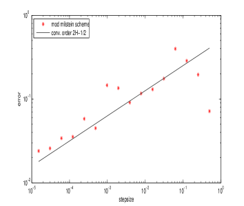
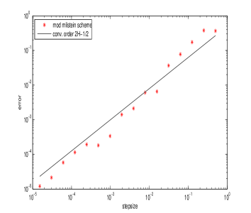
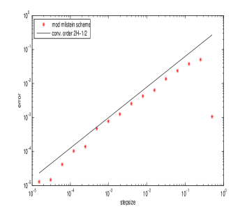
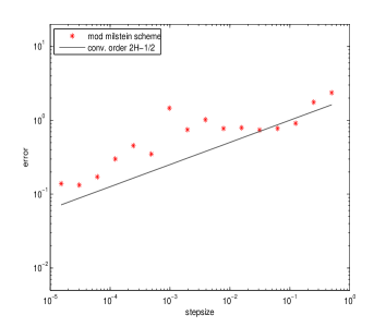
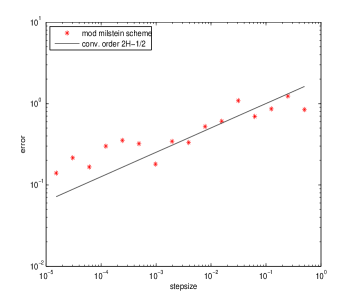
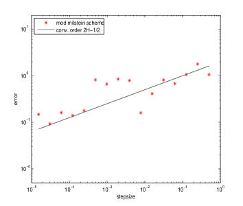
Figure 1 shows the maximum error in the discretization points, i.e.

$$\max_{k=0,\ldots,n}|Y_{kT/n}(\omega)-Z^{n}_{kT/n}(\omega)|,$$

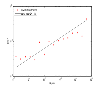
which for brevity we call in the following maximum error, versus the step size $1/n$ for four different sample paths $\omega\in\Omega$ for $H=0.4$, while Figure 2 shows the maximum error versus the step size $1/n$ for four different sample paths $\omega\in\Omega$ for $H=0.7$. (So small values on the $x$-axis correspond to small stepsizes, while small values on the $y$-axis correspond to small errors and vice versa.)

The numerical reference solution is obtained by using our Milstein-type scheme with very small stepsize. Since we use log-log-coordinates, the straight lines correspond to the convergence order $2H-1/2$. The stars correspond to the error of the Milstein-type scheme. For $H=0.4$ the estimated convergence rates are in acceptable accordance with our conjecture, while for $H=0.7$ they are in good accordance.

Figure 3. Equation (72): pathwise maximum error vs. step size for four sample paths for $H=0.4$.

Figure 4. Equation (72): pathwise maximum error vs. step size for four sample paths for $H=0.7$.

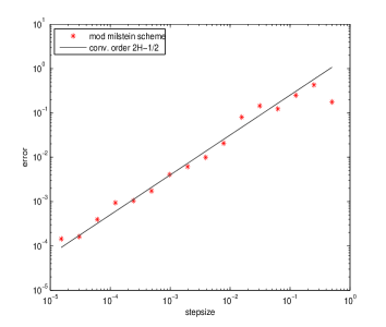
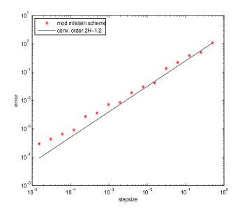
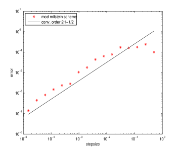
As second example we consider the linear equation

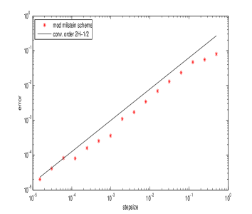
$$dY_{t}^{(1)}=Y_{t}^{(2)}dB_{t}^{(1)},\quad dY_{t}^{(2)}=Y_{t}^{(1)}dB_{t}^{(2)},\quad t\in[0,1],\qquad\,\,Y_{0}^{(1)}=1,\,Y_{0}^{(2)}=2.$$ (72)

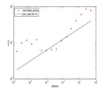
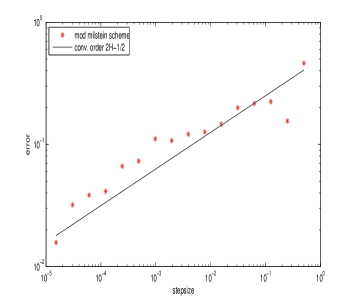
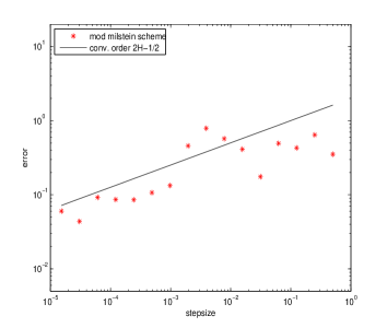
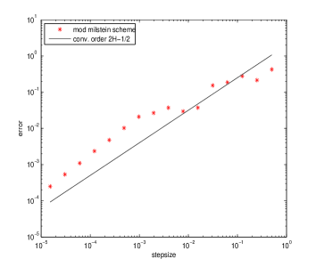
Figures 3 and 4 show again the maximum error versus the step size for four different sample paths for $H=0.4$ and $H=0.7$, respectively. Again the estimated covergence rates are in acceptable accordance with our conjecture for $H=0.4$ and in good accordance for $H=0.7$.

Note that the convergence order $2H-1/2$ is quite slow for small $H$. In particular, for $H=0.4$ the convergence order equals $0.3$. We suppose that this effect also causes the fluctuating behaviour in the estimated convergence rates in the case $H=0.4$.

6. Appendix: Proof of Theorem 2.6

6.1. Existence and uniqueness of the solution

This section gives some details of the proof of point (1) of Theorem 2.6 in the case $\gamma\leq 1/2$. The case $\gamma>1/2$ is simpler and thus omitted.

The solution to equation (15) is obtained via a fixed-point argument, which is first applied locally and then extended to the whole interval $[0,T]$.

Notations. For $\mathcal{Q}_{\kappa,a}^{x}([\ell_{1},\ell_{2}];\mathbb{R}^{d})$ we will write in the following only $\mathcal{Q}_{\kappa}^{x}([\ell_{1},\ell_{2}])$ to simplify the notation. In particular, note that the norm $\mathcal{N}[\cdot;\mathcal{Q}_{\kappa,a}^{x}([\ell_{1},\ell_{2}])]$ does not depend on $a\in\mathbb{R}^{d}$. Moreover, for $y\in\mathcal{Q}_{\kappa}^{x}([\ell_{1},\ell_{2}])$, which admits the decomposition

$$(\delta y)_{st}=\zeta_{s}(\delta\xi)_{st}+r_{st},$$

we set

$$y^{x}:=\zeta,\qquad y^{\sharp}:=r.$$

Local considerations. Consider a time $0<T_{0}\leq T$ and for any $y\in\mathcal{Q}_{\kappa}^{x}([0,T_{0}])$, define $z=\Gamma_{T_{0}}(y)$ as the unique process in $\mathcal{Q}_{\kappa}^{x}([0,T_{0}])$ such that $z_{0}=y_{0}$ and $(\delta z)_{st}=\mathcal{J}_{st}(\sigma(y)\,dx)$. If $y,\tilde{y}\in\mathcal{Q}_{\kappa}^{x}([0,T_{0}])$ with $(y_{0},y^{x}_{0})=(\tilde{y}_{0},\tilde{y}^{x}_{0})=(a,\sigma(a))$, and if $z=\Gamma_{T_{0}}(y),\tilde{z}=\Gamma_{T_{0}}(\tilde{y})$, then some standard differential calculus easily leads to

$$\mathcal{N}[z;\mathcal{Q}_{\kappa}^{x}([0,T_{0}])]\leq c_{x}\left\{1+T_{0}^{\gamma-\kappa}\mathcal{N}[y;\mathcal{Q}_{\kappa}^{x}([0,T_{0}])]^{2}\right\},$$ (73)

and

$$\mathcal{N}[z-\tilde{z};\mathcal{Q}_{\kappa}^{x}([0,T_{0}])]\\ \leq c_{x}T_{0}^{\kappa}\mathcal{N}[y-\tilde{y};\mathcal{Q}_{\kappa}^{x}([0,T_{0}])]\left\{1+\mathcal{N}[y;\mathcal{Q}_{\kappa}^{x}([0,T_{0}])]^{2}+\mathcal{N}[\tilde{y};\mathcal{Q}_{\kappa}^{x}([0,T_{0}])]^{2}\right\},$$ (74)

with $c_{x}=c(1+\lVert x\rVert_{\gamma}+\lVert\mathbf{x}^{2}\rVert_{2\gamma})$ for some constant $c>1$. Now set $T_{0}=(4c_{x}^{2})^{-1/(\gamma-\kappa)}$ and $R_{T_{0}}=2c_{x}$, so that, if in addition $\mathcal{N}[y;\mathcal{Q}_{\kappa}^{x}([0,T_{0}])]\leq R_{T_{0}}$, then by (73), $\mathcal{N}[z;\mathcal{Q}_{\kappa}^{x}([0,T_{0}])]$ $\leq R_{T_{0}}$ and, if also $\mathcal{N}[\tilde{y};\mathcal{Q}_{\kappa}^{x}([0,T_{0}])]\leq R_{T_{0}}$, by (74),

$$\mathcal{N}[z-\tilde{z};\mathcal{Q}_{\kappa}^{x}([0,T_{0}])]\leq c_{x}\,\mathcal{N}[y-\tilde{y};\mathcal{Q}_{\kappa}^{x}([0,T_{0}])]\cdot(4c_{x}^{2})^{-\kappa/(\gamma-\kappa)}\left\{1+8c_{x}^{2}\right\}.$$

Observe that $3-2\kappa/(\gamma-\kappa)<0$ for $1/3<\kappa<\gamma\leq 1/2$ and so

$$c_{x}(4c_{x}^{2})^{-\kappa/(\gamma-\kappa)}\left\{1+8c_{x}^{2}\right\}=\left(\frac{1}{4}\right)^{\kappa/(\gamma-\kappa)}\left\{c_{x}^{1-2\kappa/(\gamma-\kappa)}+8c_{x}^{3-2\kappa/(\gamma-\kappa)}\right\}\leq 9\left(\frac{1}{4}\right)^{2}<1.$$

As a result, $\Gamma_{T_{0}}$ is a strict contraction of the following closed subset of $\mathcal{Q}_{\kappa}^{x}([0,T_{0}])$:

$$\mathcal{B}_{(a,\sigma(a)),R_{T_{0}}}^{T_{0}}=\left\{y\in\mathcal{Q}_{\kappa}^{x}([0,T_{0}]);\ (y_{0},y^{x}_{0})=(a,\sigma(a))\ ,\ \mathcal{N}[y;\mathcal{Q}_{\kappa}^{x}([0,T_{0}])]\leq R_{T_{0}}\right\}.$$

Let us denote by $y^{T_{0}}$ the fixed point of the restriction of $\Gamma_{T_{0}}$ to $\mathcal{B}_{(a,\sigma(a)),R_{T_{0}}}^{T_{0}}$.

Extending the solution. One can use the same arguments as in the previous step for the set

$$\mathcal{B}_{\left(y_{T_{0}}^{T_{0}},\sigma\left(y_{T_{0}}^{T_{0}}\right)\right),R_{T_{0}}}^{2T_{0}}\\ =\left\{y\in\mathcal{Q}_{\kappa}^{x}([T_{0},2T_{0}]);\ (y_{T_{0}},y^{x}_{T_{0}})=\left(y_{T_{0}}^{T_{0}},\sigma\left(y_{T_{0}}^{T_{0}}\right)\right)\ ,\ \mathcal{N}[y;\mathcal{Q}_{\kappa}^{x}([T_{0},2T_{0}])]\leq R_{T_{0}}\right\},$$ (75)

and this provides us with an extension of the solution on $[T_{0},2T_{0}]$, denoted by $y^{2T_{0}}$. Repeat the procedure until $[0,T]$ is covered, and then define

$$y=\sum_{i=1}^{N_{T_{0}}}y^{iT_{0}}\cdot 1_{[(i-1)T_{0},iT_{0}]}\ ,\ y^{x}=\sum_{i=1}^{N_{T_{0}}}y^{x,iT_{0}}\cdot 1_{[(i-1)T_{0},iT_{0}]},$$

where $N_{T_{0}}$ is the smallest integer such that $N_{T_{0}}\cdot T_{0}\geq T$.

It is not hard to see that $y$ is a solution to the system (15). Moreover,

$$\mathcal{N}[y;\mathcal{Q}_{\kappa}^{x}([0,T])]$$

$$\leq\sup_{k=1,\ldots,N_{T_{0}}}\mathcal{N}[y^{kT_{0}};\mathcal{Q}_{\kappa}^{x}([(k-1)T_{0},kT_{0}])]+\left\{1+\lVert x\rVert_{\gamma}\right\}\sum_{k=1}^{N_{T_{0}}}\mathcal{N}[y^{kT_{0}};\mathcal{Q}_{\kappa}^{x}([(k-1)T_{0},kT_{0}])]$$

$$\leq R_{T_{0}}+R_{T_{0}}\cdot N_{T_{0}}\cdot\left\{1+\lVert x\rVert_{\gamma}\right\}\leq 2c_{x}\left(1+\left(T/T_{0}+1\right)\left(1+\lVert x\rVert_{\gamma}\right)\right)$$

$$\leq 2c_{x}\left(1+\left(1+4\cdot T\cdot c_{x}^{2/(\gamma-\kappa)}\right)\left(1+\lVert x\rVert_{\gamma}\right)\right),$$

which gives the estimate (21). The unicity of this solution is easy to prove due to (74). The details are left to the reader.

6.2. Continuity of the Itô map

We shall now prove point (2) in Theorem 2.6. For this, let us again introduce some notation:

Notation: If $y\in\mathcal{Q}_{\kappa}^{x}$ and $\tilde{y}\in\mathcal{Q}_{\kappa}^{\tilde{x}}$ for two different driving signals $x,\tilde{x}$, define

$$\mathcal{N}[y-\tilde{y};\mathcal{Q}_{\kappa}^{x,\tilde{x}}]=\mathcal{N}[(y,y^{x})-(\tilde{y},\tilde{y}^{x});\mathcal{Q}_{\kappa}^{x,\tilde{x}}]:=\mathcal{N}[y-\tilde{y};\mathcal{C}_{1}^{\gamma}]+\mathcal{N}[y^{x}-\tilde{y}^{x};\mathcal{C}_{1}^{0,\kappa}]\\ +\mathcal{N}[y^{\sharp}-\tilde{y}^{\sharp};\mathcal{C}_{2}^{2\kappa}].$$

Local considerations. Consider a time $T_{0}>0$. From the decomposition

$$\delta(y-\tilde{y})_{st}=\left[\sigma(y_{s})-\sigma(\tilde{y}_{s})\right]\cdot(\delta x)_{st}+\sigma(\tilde{y}_{s})\cdot\delta(x-\tilde{x})_{st}+\left[y^{x}_{s}\sigma^{\prime}(y_{s})-\tilde{y}^{x}\sigma^{\prime}(\tilde{y}_{s})\right]\cdot\mathbf{x}^{2}_{st}\\ {}\qquad\qquad+\tilde{y}^{x}_{s}\sigma^{\prime}(\tilde{y}_{s})\cdot\left[\mathbf{x}^{2}_{st}-\tilde{\mathbf{x}}^{2}_{st}\right]+\Lambda_{st}\big{(}\left[\sigma(y)^{\sharp}-\sigma(\tilde{y})^{\sharp}\right]\cdot\delta x+\sigma(\tilde{y})^{\sharp}\cdot\delta(x-\tilde{x})\\ +\delta\left[y^{x}\sigma^{\prime}(y)-\tilde{y}^{x}\sigma^{\prime}(\tilde{y})\right]\cdot\mathbf{x}^{2}_{st}+\delta(\tilde{y}^{x}\sigma^{\prime}(\tilde{y}))\cdot\left[\mathbf{x}^{2}-\tilde{\mathbf{x}}^{2}\right]\big{)},$$

where we have used

$$(\delta y)_{st}=\left[(\operatorname{id}-\Lambda\delta)(\sigma(y)\cdot\delta x+(\sigma(y))^{x}\cdot\mathbf{x}^{\mathbf{2}})\right]_{st},$$

some standard computations yield

$$\mathcal{N}[y-\tilde{y};\mathcal{Q}_{\kappa}^{x,\tilde{x}}([0,T_{0}])]\\ \leq c_{x,\tilde{x},y,\tilde{y}}\left\{T_{0}^{\kappa}\mathcal{N}[y-\tilde{y};\mathcal{Q}_{\kappa}^{x,\tilde{x}}([0,T_{0}])]+\lVert x-\tilde{x}\rVert_{\gamma}+\lVert\mathbf{x}^{2}-\tilde{\mathbf{x}}^{2}\rVert_{2\gamma}+\left|a-\tilde{a}\right|\right\}$$

with

$$c_{x,\tilde{x},y,\tilde{y}}=c\left\{1+\lVert x\rVert_{\gamma}+\lVert\mathbf{x}^{2}\rVert_{2\gamma}+\lVert\tilde{x}\rVert_{\gamma}+\lVert\tilde{\mathbf{x}}^{2}\rVert_{2\gamma}+\mathcal{N}[y;\mathcal{Q}_{\kappa}^{x}([0,T])]^{2}+\mathcal{N}[\tilde{y};\mathcal{Q}_{\kappa}^{\tilde{x}}([0,T])]^{2}\right\},$$

for some constant $c>0$. Now remember that $\mathcal{N}[y;\mathcal{Q}_{\kappa}^{x}([0,T])]\leq P_{T}(\lVert x\rVert_{\gamma},\lVert\mathbf{x}^{2}\rVert_{2\gamma})$, as well as $\mathcal{N}[\tilde{y};\mathcal{Q}_{\kappa}^{\tilde{x}}([0,T])]\leq P_{T}(\lVert\tilde{x}\rVert_{\gamma},\lVert\tilde{\mathbf{x}}^{2}\rVert_{2\gamma})$, for a certain polynomial function $P_{T}$, so that $c_{x,\tilde{x},y,\tilde{y}}\leq c_{x,\tilde{x}}$, where $c_{x,\tilde{x}}>0$ stands for a polynomial expression of $\lVert x\rVert_{\gamma},\lVert\mathbf{x}^{2}\rVert_{2\gamma}$ and $\lVert\tilde{x}\rVert_{\gamma},\lVert\tilde{\mathbf{x}}^{2}\rVert_{2\gamma}$. Set $T_{0}=(2c_{x,\tilde{x}})^{-1/\kappa}$ and in this way

$$\mathcal{N}[y-\tilde{y};\mathcal{Q}_{\kappa}^{x,\tilde{x}}([0,T_{0}])]\leq 2c_{x,\tilde{x}}\left\{\lVert x-\tilde{x}\rVert_{\gamma}+\lVert\mathbf{x}^{2}-\tilde{\mathbf{x}}^{2}\rVert_{2\gamma}+\left|a-\tilde{a}\right|\right\}.$$

Extending the inequality. With the same arguments as in the above step, we get, for any $k\geq 1$,

$$\mathcal{N}[y-\tilde{y};\mathcal{Q}_{\kappa}^{x,\tilde{x}}([kT_{0},(k+1)T_{0}])]$$

$$\leq 2c_{x,\tilde{x}}\left\{\lVert x-\tilde{x}\rVert_{\gamma}+\lVert\mathbf{x}^{2}-\tilde{\mathbf{x}}^{2}\rVert_{2\gamma}+\left|y_{kT_{0}}-\tilde{y}_{kT_{0}}\right|\right\}$$

$$\leq 2c_{x,\tilde{x}}\left\{\lVert x-\tilde{x}\rVert_{\gamma}+\lVert\mathbf{x}^{2}-\tilde{\mathbf{x}}^{2}\rVert_{2\gamma}+\left|a-\tilde{a}\right|+T_{0}^{\kappa}\sum_{l=0}^{k-1}\mathcal{N}[y-\tilde{y};\mathcal{Q}_{\kappa}^{x,\tilde{x}}([lT_{0},(l+1)T_{0}])]\right\}$$

and as a result

$$\mathcal{N}[y-\tilde{y};\mathcal{Q}_{\kappa}^{x,\tilde{x}}([kT_{0},(k+1)T_{0}])]\leq 2c_{x,\tilde{x}}\cdot e^{k}\left\{\lVert x-\tilde{x}\rVert_{\gamma}+\lVert\mathbf{x}^{2}-\tilde{\mathbf{x}}^{2}\rVert_{2\gamma}+\left|a-\tilde{a}\right|\right\}$$

using the discrete version of Gronwall’s Lemma.

Inequality (22) is then a direct consequence of

$$\mathcal{N}[y-\tilde{y};\mathcal{C}_{1}^{\gamma}([0,T])]\leq\sum_{k=0}^{N_{T_{0}}-1}\mathcal{N}[y-\tilde{y};\mathcal{Q}_{\kappa}^{x,\tilde{x}}([kT_{0},(k+1)T_{0}])],$$

where $N_{T_{0}}$ is the smallest integer such that $N_{T_{0}}\cdot T_{0}\geq T$, so that $N_{T_{0}}\leq 1+T/T_{0}\leq 1+T\cdot(2c_{x,\tilde{x}})^{\kappa}$.

References

- [1] F. Baudoin, L. Coutin: Operators associated with a stochastic differential equation driven by fractional Brownian motions. Stochastic Process. Appl. 117(5) (2007), 550–574.
- [2] C. Bender, T. Sottinen, E. Valkeila: Pricing by Hedging and No-Arbitrage beyond Semimartingales. Finance Stoch. 12 (2008), 441–468.
- [3] T. Björk, H. Hult: A note on Wick products and the fractional Black-Scholes model. Finance Stoch. 9 (2005), 197–209.
- [4] T. Cass, P. Friz, N. Victoir: Non-degeneracy of Wiener functionals arising from rough differential equations. Trans. Amer. Math. Soc. 361 (2009), 3359–3371.
- [5] S. Chang, S. Li, M. Chiang, S. Hu, M. Hsyu: Fractal dimension estimation via spectral distribution function and its application to physiological signals. IEEE Trans. Biol. Engineering 54(10) (2007), 1895–1898.
- [6] L. Coutin, Z. Qian: Stochastic rough path analysis and fractional Brownian motion. Probab. Theory Relat. Fields 122 (2002), 108–140.
- [7] J.M. Corcuera: Power variation analysis of some integral long-memory processes. In: F.E. Benth (ed.) et al., Stochastic analysis and applications. Springer. Abel Symposia 2, 219–234 (2007).
- [8] N.J. Cutland, P.E. Kopp, W. Willinger: Stock price returns and the Joseph effect: A fractional version of the Black-Scholes model. In: E. Bolthausen (ed.) et al., Seminar on stochastic analysis, random fields and applications. Birkhäuser. Prog. Probab. 36, 327–351 (1995).
- [9] A. Davie: Differential equations driven by rough paths: an approach via discrete approximation. Appl. Math. Res. Express. (2007), No. 2, 40 pp.
- [10] L. Decreusefond, D. Nualart: Flow properties of differential equations driven by fractional Brownian motion. In: P.H. Baxendale (ed.) et al., Stochastic differential equations: theory and applications. World Sci. Publ. Interdiscip. Math. Sci. 2, 249–262 (2007).
- [11] A. Deya, S. Tindel: Rough Volterra equations 2: convolutional generalized integrals. Arxiv Preprint (2008).
- [12] G. Denk, D. Meintrup, S. Schäffler: Transient noise simulation: Modeling and simulation of -noise. In: Antreich, K. (ed.) et al., Modeling, simulation, and optimization of integrated circuits. Birkhäuser. Int. Ser. Numer. Math. 146, 251–267 (2001).
- [13] G. Denk, R. Winkler: Modelling and simulation of transient noise in circuit simulation. Math. Comput. Model. Dyn. Syst. 13(4) (2007), 383–394.
- [14] J. Hüsler, V. Piterbarg, O. Seleznjev: On convergence of the uniform norms for Gaussian processes and linear approximation problems. Ann. Appl. Probab. 13(4) (2003), 1615–1653.
- [15] D. Feyel, A. de La Pradelle. Curvilinear integrals along enriched paths. Electron. J. Probab. 11 (2006), 860–892.
- [16] P. Friz, N. Victoir: Multidimensional stochastic processes as rough paths: theory and applications. Cambridge University Press, to appear.
- [17] P. Guasoni. No arbitrage under transaction costs, with fractional Brownian motion and beyond. Math. Finance 16 (2006), 569–582.
- [18] M. Gubinelli: Controlling rough paths. J. Funct. Anal. 216 (2004), 86-140.
- [19] M. Gubinelli, S. Tindel: Rough evolution equations. Arxiv Preprint (2008), to appear in Ann. Prob.
- [20] M. Hairer, A. Ohashi: Ergodic theory for SDEs with extrinsic memory. Ann. Probab. 35(5) (2007), 1950–1977.
- [21] A. Jentzen, P. Kloeden, A. Neuenkirch: Pathwise approximation of stochastic differential equations on domains: Higher order convergence rates without global Lipschitz coefficients. Numer. Math. 112(1) (2009), 41–64.
- [22] P. Kloeden, E. Platen: Numerical Solution of Stochastic Differential equations. Springer, 3rd edition. (2009)
- [23] S. Kou: Stochastic modeling in nanoscale Physics: subdiffusion within proteins. Ann. Appl. Stat. 2(2) (2008), 501–535.
- [24] S. Kou, X. Sunney-Xie: Generalized Langevin equation with fractional Gaussian noise: subdiffusion within a single protein molecule. Phys. Rev. Lett. 93, no. 18 (2004).
- [25] T. Lyons, Z. Qian: System control and rough paths. Oxford University Press. (2002)
- [26] Y. Mishura, G. Shevchenko: The rate of convergence for Euler approximations of solutions of stochastic differential equations driven by fractional Brownian motion. Stochastics 80(5) (2008), 489–511.
- [27] T. Müller-Gronbach, K. Ritter: Minimal errors for strong and weak approximation of stochastic differential equations. In: A. Keller (ed.) et al., Monte Carlo and quasi-Monte Carlo methods 2006. Springer. 53–82 (2008).
- [28] A. Neuenkirch, I. Nourdin: Exact rate of convergence of some approximation schemes associated to SDEs driven by a fractional Brownian motion. J. Theoret. Probab. 20(4) (2007), 871–899.
- [29] A. Neuenkirch, I. Nourdin, A. Rößler, S. Tindel: Trees and asymptotic developments for fractional diffusion processes. Ann. Inst. Poincaré (B), Prob. and Stat. 45(1) (2009), 157–174.
- [30] A. Neuenkirch, I. Nourdin, S. Tindel: Delay equations driven by rough paths. Elec. J. Probab. 13 (2008), 2031–2068.
- [31] A. Neuenkirch, S. Tindel, J. Unterberger: Discretizing the Lévy area. To appear in Stochastic Process. Appl.
- [32] D. Nualart: The Malliavin Calculus and Related Topics. Springer, 2nd edition. (2006)
- [33] D. Nualart, A. Rǎşcanu: Differential equations driven by fractional Brownian motion. Collect. Math. 53(1) (2002), 55–81.
- [34] D. Odde, E. Tanaka, S. Hawkins, H. Buettner: Stochastic dynamics of the nerve growth cone and its microtubules during neurite outgrowth. Biotechnol. and Bioeng. 50(4) (1996), 452–461.
- [35] S. Tindel, J. Unterberger: The rough path associated to the multidimensional analytic fbm with any Hurst parameter. Arxiv Preprint (2008).
- [36] K. Twardowska: Wong-Zakai approximations for stochastic differential equations. Acta Appl. Math. 43(3) (1996), 317–359.
- [37] J. Unterberger: Stochastic calculus for fractional Brownian motion with Hurst exponent : a rough path method by analytic extension. Ann. Prob. 37(2) (2009), 565–614.
- [38] W. Wang: On a functional limit result for increments of a fractional Brownian motion. Acta Math. Hung. 93(1-2) (2001), 153–170.
- [39] W. Willinger, M.S. Taqqu, V. Teverovsky: Stock market prices and long-range dependence. Finance Stoch. 3(1) (1999), 1–13.
- [40] M. Zähle: Integration with respect to fractal functions and stochastic calculus I. Probab. Theory Relat. Fields 111 (1998), 333–374.