Many-body localization transition in a lattice model of interacting fermions :
statistics of renormalized hoppings in configuration space

Abstract

We consider the one-dimensional lattice model of interacting fermions with disorder studied previously by Oganesyan and Huse [Phys. Rev. B 75, 155111 (2007)]. To characterize a possible many-body localization transition as a function of the disorder strength $W$, we use an exact renormalization procedure in configuration space that generalizes the Aoki real-space RG procedure for Anderson localization one-particle models [H. Aoki, J. Phys. C13, 3369 (1980)]. We focus on the statistical properties of the renormalized hopping $V_{L}$ between two configurations separated by a distance $L$ in configuration space (distance being defined as the minimal number of elementary moves to go from one configuration to the other). Our numerical results point towards the existence of a many-body localization transition at a finite disorder strength $W_{c}$. In the localized phase $W>W_{c}$, the typical renormalized hopping $V_{L}^{typ}\equiv e^{\overline{\ln V_{L}}}$ decays exponentially in $L$ as $(\ln V_{L}^{typ})\simeq-\frac{L}{\xi_{loc}}$ and the localization length diverges as $\xi_{loc}(W)\sim(W-W_{c})^{-\nu_{loc}}$ with a critical exponent of order $\nu_{loc}\simeq 0.45$. In the delocalized phase $W<W_{c}$, the renormalized hopping remains a finite random variable as $L\to\infty$, and the typical asymptotic value $V_{\infty}^{typ}\equiv e^{\overline{\ln V_{\infty}}}$ presents an essential singularity $(\ln V_{\infty}^{typ})\sim-(W_{c}-W)^{-\kappa}$ with an exponent of order $\kappa\sim 1.4$. Finally, we show that this analysis in configuration space is compatible with the localization properties of the simplest two-point correlation function in real space.

I Introduction

Whereas Anderson localization phenomena [1] are rather well understood for a single particle (see the reviews [2, 3, 4]), the case of interacting particles in a random potential has remained much more challenging (see the review [5]). In the field of disordered fermions, there has been for instance a lot of works on quantum Coulomb glasses (see for instance [6, 7, 8] and references therein), including the debate on the existence of a metal-insulator transition for interacting electrons in two dimensions (see [9, 10, 11] and references therein). In the field of disordered bosons, many studies have been devoted to the existence and properties of the superfluid-insulator transition (see [12, 13, 14, 15, 16, 17] and references therein). Recently, the idea to reformulate the many-body localization problem as an Anderson localization problem in Fock space or in Hilbert space has been very useful [18, 19, 20, 21, 22, 23, 24, 25]. In particular, this type of analysis has led to the prediction that the conductivity of interacting electrons models could exactly vanish in some finite region of parameters in the absence of any external continuous bath [24, 25]. The reason is that conduction mechanisms based on variable-range hopping need a continuous bath to locally supply or absorb energy to permit hopping between levels which are not exactly degenerate. Since quantum levels are discrete, the many-particle system can fail to be an effective heat-bath for itself. Following these ideas, Oganesyan and Huse have proposed that this type of many-body localization transition could be realized in some one-dimensional lattice models of interacting fermions [26]. Unfortunately, the numerical study concerning the spectral statistics alone presented in Ref. [26] has turned out to be not completely conclusive as a result of very strong finite-size effects. Moreover, the analogy with Anderson localization on high dimensional and Cayley tree indicates that criteria based on the level repulsion may not be very appropriate in this case [26]. In the present paper, we propose to study the existence of a many-body localization transition in the very same model of Ref. [26] by studying another type of observable which contains some information on the localization of eigenstates. More precisely, we use an exact renormalization procedure in configuration space to compute numerically the renormalized hopping between two configurations as a function of their distance in configuration space. We present numerical results on the statistical properties of this renormalized hopping that point towards the existence of a many-body localization transition at a finite disorder strength. In the localized phase, we measure a power-law divergence of the localization length. In the delocalized phase, we measure an essential singularity for the asymptotic renormalized hopping. These scaling laws are thus reminiscent of the Anderson localization transition on the Cayley tree, which is the simplest example of Anderson transition in a space of infinite dimension, but the values of exponents are different.

The paper is organized as follows. In Section II, we describe how many-body localization models can be studied numerically via an exact renormalization procedure (’RG’) in configuration space that generalizes Aoki real-space RG procedure for Anderson localization one-particle models. In Section III, we present our numerical results for a one-dimensional lattice model of interacting fermions. In section IV, we discuss the similarities and differences with the scaling laws of Anderson localization on the Cayley tree, and propose a specific form of finite-size scaling analysis. In section V, we present independent numerical results concerning the simplest real-space two-point correlation function, to test the compatibility with our results obtained in configuration space. Our conclusions are summarized in section VI.

II Exact renormalization procedure in configuration space

In this section, we briefly summarize the Aoki real space renormalization (’RG’) method for one-particle localization models before we describe its generalization for many-body problems.

II.1 Reminder on Aoki real space RG for one-particle localization models

For Anderson localization models, there exists an exact real-space renormalization procedure at fixed energy $E$ which preserves the Green functions of the remaining sites [27, 28, 29, 30, 31, 32].

The renormalization (RG) procedure can be applied to any Anderson localization model of the generic form

$$H=\sum_{i,j}V_{i,j}|i><j|$$ (1)

where $V_{i,i}$ is the on-site energy of site $i$, and where $V_{i,j}$ is the hopping between the sites $i$ and $j$. Upon the elimination of site $i_{0}$ in the Schrödinger equation at energy $E$

$$E\psi(i_{0})=V_{i_{0},i_{0}}\psi(i_{0})+\sum_{j\neq i_{0}}V_{i_{0},j}\psi(j)$$ (2)

the remaining sites satisfy the Schrödinger equation at energy $E$ with the renormalized parameters

$$V_{i,j}^{new}=V_{i,j}+\frac{V_{i,i_{0}}V_{i_{0},j}}{E-V_{i_{0},i_{0}}}$$ (3)

These renormalization equations are exact since they are based on elimination of the variable $\psi(i_{0})$ in the Schrödinger Equation. As stressed by Aoki [27, 28], the RG rules preserve the Green function for the remaining sites. This means for instance that if external leads are attached to all surviving sites, the scattering properties will be exactly determined using the renormalized parameters (see [32] for more details). In particular, the renormalized hopping between the last two surviving sites (after all other sites have been decimated) determines the two-point Landauer transmission between leads attached to these two points [32] : it decays exponentially with the distance in the localized phase, it remains finite in the delocalized phase, and at the critical point it becomes multifractal.

II.2 Generalization in configuration space for many-body localization models

The above RG procedure has the following natural generalization for many-body models. Let us denote ${\cal C}$ a configuration of the many-body problem to write the Hamiltonian as

$$H_{many}=\sum_{{\cal C}_{i},{\cal C}_{j}}V_{{\cal C}_{i},{\cal C}_{j}}|{\cal C}_{i}><{\cal C}_{j}|$$ (4)

Then the Schrödinger equation projected onto the configuration ${\cal C}_{i_{0}}$

$$E\psi({\cal C}_{i_{0}})=\sum_{{\cal C}_{j}}V_{{\cal C}_{i_{0}},{\cal C}_{j}}\psi({\cal C}_{j})$$ (5)

allows to eliminate $\psi({\cal C}_{i_{0}})$. The remaining configurations satisfy the Schrödinger equation with renormalized parameters

$$V_{{\cal C}_{i},{\cal C}_{j}}^{new}=V_{{\cal C}_{i},{\cal C}_{j}}+\frac{V_{{\cal C}_{i},{\cal C}_{i_{0}}}V_{{\cal C}_{i_{0}},{\cal C}_{j}}}{E-V_{{\cal C}_{i_{0}},{\cal C}_{i_{0}}}}$$ (6)

These rules in configuration space have been already used for the two-particle 1D Anderson tight-binding model [33]. In the following, we apply them to a model of interacting fermions that we now describe.

II.3 Application to the interacting fermions model of Ref. [26]

In numerical studies of quantum problems containing both interactions and disorder, it is natural to consider first the spatial dimension $d=1$. The simplest model is then a chain of spinless fermions with nearest-neighbor interaction and on-site disorder (see for instance [34, 35, 36] and references therein). This type of model can also be studied in the language of quantum spin chains as in Ref. [37], where a powerful time-dependent Density Matrix Renormalization Group method has been used to characterize the many-body localized phase. In this paper, we consider the same class of model, but with second-neighbor hopping in addition, as in Ref. [26]. More precisely, the model of Ref. [26] is defined by the following Hamiltonian on a one-dimensional lattice of $L$ sites with periodic boundary conditions

$$H=\sum_{i=1}^{L}\left[w_{i}n_{i}+V\left(n_{i}-\frac{1}{2}\right)\left(n_{i+1}-\frac{1}{2}\right)+c_{i}^{\dagger}c_{i+1}+c_{i+1}^{\dagger}c_{i}+c_{i}^{\dagger}c_{i+2}+c_{i+2}^{\dagger}c_{i}\right]$$ (7)

with the usual notations :

(i) $n_{i}=c_{i}^{\dagger}c_{i}$ represents the number of spinless fermion on site $i$ and can take only two values ($0$ if the site is empty or $1$ if the site is occupied). The many-body Hilbert space has thus for dimension

$${\cal N}_{L}=2^{L}$$ (8)

The spinless character has been chosen to reach bigger sizes $L$ for a given value of the Hilbert space dimension ${\cal N}_{L}$ [26].

(ii) the on-site energies $w_{i}$ are independent Gaussian variables with zero mean and variance $W^{2}$, i.e. $W$ measures the disorder strength (we have not used the ’microcanonical constraint’ of Ref. [26] consisting in the requirement that $(1/L)\sum w_{i}^{2}$ should be exactly $W^{2}$ to reduce statistical uncertainties).

(iii) the nearest-neighbor interaction is chosen to be $V=2$, the hopping terms between nearest-neighbors and second-neighbors are chosen to be $t=t^{\prime}=1$. The second-neighbor hopping is included to have non-integrability at zero randomness, see [38] for more details on the properties of the model in the zero-disorder limit.

(iv) the total number of particles is conserved : we study the case of half-filling with $L/2$ particles for $L$ sites as in [26]. The dimension of the Hilbert space is then given by the binomial coefficient

$${\cal N}_{L}^{half-filling}=\binom{L}{\frac{L}{2}}\mathop{\propto}_{L\to+\infty}\frac{2^{L}}{\sqrt{L}}$$ (9)

Physically, the important point is that at leading order, it still grows exponentially in $L$.

In summary, we consider in this paper the model of Ref. [26] with exactly the same values of parameters, but we study another observable to detect the possible many-body localization transition. We have applied the RG procedure in configuration space described above, to obtain, in each disordered sample of even size $L$, the renormalized hopping $V_{L}$ at some energy $E$ between two configurations ${\cal C}_{A},$ and ${\cal C}_{B}$ after the decimation of all other configurations

$$V_{L}\equiv V_{{\cal C}_{A},{\cal C}_{B}}(E)$$ (10)

We have made the following choices :

(c1) we consider the zero-energy case $E=0$, because it represents the center of the many-body energy levels. Indeed, in Anderson localization models, it is well known that energy levels near the center are the more favourable to delocalization : if these states are localized, one expects that all other states will also be localized.

(c2) we have chosen the following configurations : the configuration ${\cal C}_{A}$ has all even sites occupied and all odd sites empty, whereas the configuration ${\cal C}_{B}$ has all odd sites occupied and all even sites empty. Their distance in configuration space is thus $L/2$ (the minimal path to go from configuration ${\cal C}_{A}$ to configuration ${\cal C}_{B}$ requires $L/2$ elementary moves). In the absence of disorder, the model is known to be conducting (see [38] for a detailed study of conductivity properties) ; the two configurations ${\cal C}_{A}$ and ${\cal C}_{B}$ are equivalent up to a translation of one lattice site, and are thus expected to be connected by a finite renormalized hopping. In the presence of disorder, these two configurations are not equivalent anymore, and one expects that the renormalized hopping $V_{L}$ will become exponentially small in $L$ for sufficiently strong disorder.

This choice (c2) of alternate configurations ${\cal C}_{A}$ and ${\cal C}_{B}$ can be questioned in various ways. For instance, if one wishes to maximize the distance in Fock space, one obtains the configurations where all particles are on the first half or on the second half : physically, it is however clear that these two configurations are not typical because they are extremely inhomogeneous and because only 4 particles (2 particles at each boundary of the macroscopic cluster) can move for arbitrary large $L$ (instead of an extensive number of particles for typical configurations). More generally, in contrast to usual Anderson localization models where all sites are equivalent, a new difficulty that arises in many-body localization models is that all configurations are not equivalent : configurations have different hopping connectivities, and different interaction energies, so that the configuration space has already an inhomogeneous structure even before the introduction of disorder variables. Since an extensive study of the renormalized hoppings in this complicated configuration space is not really possible, we have decided to consider only the choice (c2) of alternate configurations ${\cal C}_{A}$ and ${\cal C}_{B}$ in the remaining of this paper. However, to show that our results are meaningful and do not really depend of our precise choice (c2), we present in section V independent numerical results concerning the simplest real-space two-point correlation function.

III Numerical results for the interacting fermions model of Ref. [26]

In this section, we describe our numerical results concerning the statistics of $V_{L}$ at $E=0$ between the alternate configurations ${\cal C}_{A}$ and ${\cal C}_{B}$ described above for even sizes $4\leq L\leq 12$ with corresponding statistics $15.10^{7}\leq n_{s}(L)\leq 3650$ of disordered samples (we have also data corresponding to $L=14$ with $n_{s}=100$ samples, but this statistics has turned out to be insufficient for most purposes).

III.1 Analysis of the localized phase

Figure 1: (Color on line) Statistics of the renormalized hopping $V_{L}$ in the localized phase (data for the disorder strength $W=20$) : (a) Probability distribution $P_{L}(\ln V_{L})$ of the logarithm of renormalized hopping $V_{L}$ for the sizes $L=4,6,8,10,12$. (b) same data for the rescaled variable $x$ of Eq. 11 for the sizes $L=6,8,10,12$ : the convergence towards a fixed rescaled distribution ${\tilde{P}}(x)$ is rapid (we have only excluded the smallest size $L=4$ that was too different).

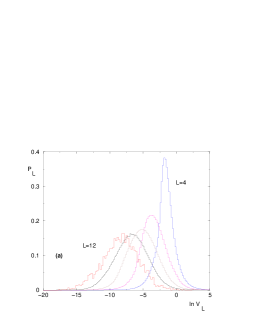
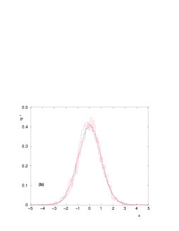
For strong disorder, we find that the renormalized hopping $V_{L}$ introduced in Eq. 10 flows towards smaller and smaller values as $L$ increases. As an example for $W=20$, we show on Fig. 1 the probability distributions $P_{L}(\ln V_{L})$ of the variable $\ln V_{L}$ over the disordered samples of a given size $L=4,6,8,10,12$ : the regular shift of these histograms towards smaller values is clear. We show on Fig. 1 (b) the same data for the rescaled variable

$$x\equiv\frac{\ln V_{L}-\overline{\ln V_{L}}}{\Delta_{L}}$$ (11)

where $\overline{\ln V_{L}}$ is the averaged value and where $\Delta_{L}$ is the width of the distribution $P_{L}(\ln V_{L})$. One can see on Fig. 1 (b) that the histograms of the rescaled variable $x$ coincide within statistical fluctuations for $L=6,8,10,12$ (we have only excluded the smallest size $L=4$ that was too different) : this shows that the convergence towards a stable rescaled distribution ${\tilde{P}}(x)$ is rapid for this model.

Figure 2: (Color on line) Exponential decay of the typical renormalized hopping $V_{L}^{typ}\equiv e^{\overline{\ln V_{L}}}$ in the localized phase : (a) Linear decay of $\overline{\ln V_{L}}$ as a function of $L$ (see Eq. 12). (b) Behavior of the slope $1/\xi_{loc}(W)$ (inverse of the localization length $\xi_{loc}(W)$ of Eq. 12) as a function of the disorder strength $W$

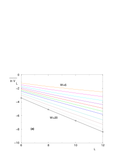
We show on Fig. 2 (a) the decay with $L$ of the disorder-average $\overline{\ln V_{L}}$ for various disorder strengths in the range $6\leq W\leq 20$ : these curves correspond to an exponential decay of the typical value $V_{L}^{typ}\equiv e^{\overline{\ln V_{L}}}$ with respect to the distance $(L/2)$ in configuration space

$$\ln(V_{L}^{typ})\equiv\overline{\ln V_{L}(W>W_{c})}\ \mathop{\simeq}_{L\to\infty}-\frac{(L/2)}{\xi_{loc}(W)}$$ (12)

where $\xi_{loc}(W)$ represents the localization length that diverges at the delocalization transition

$$\xi_{loc}(W)\mathop{\simeq}_{W\to W_{c}^{+}}(cst)(W-W_{c})^{-\nu_{loc}}$$ (13)

We show on Fig. 2 (b) our numerical result for the slope $1/\xi_{loc}(W)$ as a function of the disorder strength $W$ in the region $6\leq W\leq 20$ (below $W=6$ we cannot estimate the linear slope anymore). A three-parameter fit of the form of Eq. 13 yields a critical point in the range

$$5.2\leq W_{c}\leq 5.9$$ (14)

and a critical exponent around

$$\nu_{loc}\simeq 0.45$$ (15)

III.2 Analysis of the delocalized phase

Figure 3: (Color on line) Statistics of the renormalized hopping $V_{L}$ in the delocalized phase (a) For the disorder strength $W=2$, the probability distribution $P_{L}(\ln V_{L})$ of the logarithm of renormalized hopping $V_{L}$ remains the same for the sizes $L=8,10,12$ (we have excluded the smallest sizes $L=4,6$ that were a bit different). This should be compared with Fig. 1 (a) corresponding to the localized phase. (b) Behavior of the typical asymptotic renormalized hopping $V_{\infty}^{typ}\equiv e^{\overline{\ln V_{\infty}}}$ : $\ln V_{\infty}^{typ}=\overline{\ln V_{\infty}}$ as a function of the disorder strength $W$.

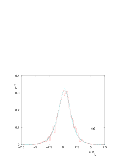
For weak disorder, we find that the renormalized hopping $V_{L}$ introduced in Eq. 10 remains a finite random variable $V_{\infty}$ finite as $L$ increases. As an example for $W=2$, we show on Fig. 3 the probability distributions $P_{L}(\ln V_{L})$ of the variable $\ln V_{L}$ over the disordered samples of a given size $L=8,10,12$ (for clarity we have excluded the smallest sizes $L=4,6$ that were too different) : it is clear that these histograms coincide up to statistical fluctuations. This should be compared with Fig. 1 (a) corresponding to the localized phase for $W=20$. In the delocalized phase, the typical renormalized hopping $V_{\infty}^{typ}\equiv e^{\overline{\ln V_{\infty}}}$ thus remains finite

$$\overline{\ln V_{L}(W<W_{c},L)}\mathop{\simeq}_{L\to\infty}\overline{\ln V_{\infty}(W<W_{c})}\ \ \ {\rm finite}$$ (16)

We show on Fig. 3 (b) our numerical estimates of the asymptotic value $\overline{\ln V_{\infty}(W<W_{c})}$ as a function of $W$. We find that our data are compatible with an essential singularity behavior of the typical asymptotic hopping $V_{\infty}^{typ}$

$$\ln V_{\infty}^{typ}(W<W_{c})\equiv\overline{\ln V_{\infty}(W<W_{c})}\mathop{\simeq}_{W\to W_{c}^{-}}-(cst)(W_{c}-W)^{-\kappa}$$ (17)

A three-parameter fit of this form yields a critical point in the range

$$5.5\leq W_{c}\leq 5.7$$ (18)

and an essential singularity exponent around

$$\kappa\simeq 1.4$$ (19)

Essential singularities in transport properties have already been found in various disordered models, in particular in Anderson localization on the Cayley tree (see [41, 45] and references therein) and in superfluid-insulator transitions of disordered bosons (see [12, 13, 14, 16] and references therein).

III.3 Conclusion of the numerical study

Figure 4: Critical behaviors obtained for a critical point at the value $W_{c}=5.6$ (a) Localized phase $W>W_{c}$ : the plot of $\ln(1/\xi_{loc}(W))$ as a function of $\ln(W-W_{c})$ corresponds to the slope $\nu_{loc}\simeq 0.45$ (see Eq. 13) (b) Delocalized phase $W<W_{c}$ : the plot of $\ln(-\overline{\ln V_{\infty}})$ as a function of $\ln(W_{c}-W)$ corresponds to the slope $\kappa\simeq 1.4$ (see Eq. 17)

In summary, our numerical data are compatible with a many-body localization transition for the model of Eq. 7. The global best value for the critical point seems to be

$$W_{c}\simeq 5.6$$ (20)

which is somewhat smaller than the critical value suggested by the level statistics study of Ref. [26]. A possible reason for this slight difference could be that the level statistics study of Ref. [26] is based on all levels of all energies, that could mix contributions of various types of states (delocalized, localized, and critical), whereas we have chosen to work at the fixed energy $E=0$ (center of the many-body energy levels). Anyway, taking into account the large uncertainties on $W_{c}$ as estimated from small system sizes, we feel that the two studies point towards the same region of disorder strength $W$.

For the value of Eq. 20, we show the log-log plots of the critical behaviors on Fig. 4. On Fig. 4 (a), we show the divergence of the localization length $\xi_{loc}(W)$ in the localized phase $W>W_{c}$ : the slope $\nu_{loc}\simeq 0.45$ (see Eq. 13). On Fig. 4 (b), we show the essential singularity of the typical asymptotic hopping in the delocalized phase $W<W_{c}$ : the slope corresponds to the exponent $\kappa\simeq 1.4$ (see Eq. 17). Of course, these values are not expected to be precise, since they have been obtained from small system sizes and some fitting/extrapolation procedures from the raw data. Nevertheless, the emergence of reasonable scaling laws is encouraging. In the following section, we discuss the similarity with the scaling laws that appear for Anderson localization on the Cayley tree.

IV Discussion : similarities and differences with Anderson localization on the Cayley tree

IV.1 Analogy with Anderson localization on the Cayley tree

As recalled in the introduction, the reformulation of the many-body localization problem as an Anderson localization problem in Fock space or in Hilbert space has been very useful [18, 19, 20, 21, 22, 23, 24, 25]. The idea is to analyse whether there exists an Anderson localization in configuration space, and to study the consequences for real-space properties. The geometry of configuration space is usually very different from the regular finite-dimensional lattices considered in Anderson one-particle localization models, and has been argued to be qualitatively similar to the Cayley tree [18, 19, 21, 24]. Since Anderson localization on the Cayley tree has been studied for a long time as a mean-field limit [39, 40, 41, 42, 43, 44, 45], results and methods have been then borrowed to analyse many-body localization properties of quantum dots [18, 19, 21, 24]. This approximation by a tree structure has been however sometimes criticized [20]. Indeed, in many-body localization models, the Fock space or Hilbert space is never exactly a tree, and thus the approximation by a Cayley tree has been proposed as a simplifying approximation to obtain an exactly solved model [18] (note however that in [24], it has been argued that an effective Cayley tree structure should actually well capture the properties of low-dimensional electronic models). But independently of the technical convenience of the tree structure, we believe that the physically important property in this analogy is the ’infinite-dimension’ property, defined as the exponential growth of the configuration space ${\cal N_{L}}$ with the real-space linear size $L$

$${\cal N}_{L}\propto e^{(cst)L}$$ (21)

(whereas in finite dimension $d$, the configuration space of a single particle grows as a power-law ${\cal N}_{L}\propto L^{d}$). As argued in [46], it is the exponential growth of Eq. 21 which is directly responsible for the presence of essential singularities of transport properties, whereas finite-dimensional lattices are characterized by power-law singularities. From the point of view of Anderson one-particle models, the Cayley tree is thus rather ’pathological’ since $d=\infty$ turns out to be a singular point, and the upper critical dimension is considered to be $d_{c}=+\infty$ [46]. From the point of view of many-body localization however, the exponential growth of Eq. 21 is the rule (see for instance Eq. 8), and thus the scaling behaviors that appear on the Caylee tree are instructive, as an example of Anderson localization on a space of infinite dimension. In particular, this analysis suggests some specific form of finite-size scaling as we now recall.

IV.2 Specific form of finite-size scaling in the critical region

Figure 5: (Color on line) Finite-size scaling analysis of our numerical data for the sizes $L=8$ (triangles), $L=10$ (squares) and $L=12$ (circles) according to the form of Eq. 22 with the values $\rho=0.76$ (see Eq. 28) and $\nu_{FS}=1.85$ (see Eq. 25) : this plot is rather convincing at criticality and in the localized phase $W>W_{c}$, whereas stronger corrections to scaling seem to be present in the delocalized phase $W<W_{c}$.

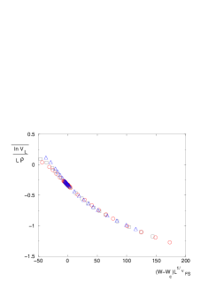
As in our recent study of the Landauer transmission for Anderson localization on the Cayley tree [45], it is natural to assume some finite-size scaling in the critical region of the form

$$\overline{\ln V_{L}(W)}\mathop{\simeq}-L^{\rho}G\left(L^{1/\nu_{FS}}(W_{c}-W)\right)$$ (22)

where the finite-size scaling exponent $\nu_{FS}$ is different from the localization length exponent $\nu_{loc}$. (This is in contrast with the scaling theory of localization in finite dimension $d$, where the finite-size scaling is governed by $\nu_{loc}$).

The matching of Eq. 22 with the localized phase (see Eq. 12 and Eq. 13) yields

$$\nu_{loc}=(1-\rho)\nu_{FS}$$ (23)

and the matching with the delocalized phase (Eq. 17) yields

$$\kappa=\rho\nu_{FS}$$ (24)

By consistence, the finite-size correlation length exponent $\nu_{FS}$ is then given by

$$\nu_{FS}=\nu_{loc}+\kappa$$ (25)

In an exactly solved travelling/non-travelling phase transition where the same type of finite-size scaling occurs [47], the physical interpretation of the finite-size scaling exponent $\nu_{FS}$ is that it governs the relaxation rate towards the finite value in the non-travelling phase. For Anderson localization on the Cayley tree, we have checked that this interpretation holds [45]. For the present many-body localization transition, this property cannot be checked with our numerical data limited to small sizes.

Exactly at criticality, we thus expect the following stretched exponential decay of the typical renormalized hopping

$$\overline{\ln V_{L}(W_{c})}\simeq-L^{\rho}$$ (26)

where the exponent $\rho$ is related to the other exponents by (see the scaling relations of Eqs 23 and 24 )

$$\rho=\frac{\kappa}{\nu_{FS}}=\frac{\kappa}{\kappa+\nu_{loc}}$$ (27)

From our previous estimates of the exponents $\nu_{loc}\simeq 0.45$ (Eq. 15) and $\kappa\simeq 1.4$ (Eq. 19), this would correspond to a numerical value of order

$$\rho\simeq 0.76$$ (28)

We show on Fig. 5 the finite-size scaling analysis of our numerical data according to the form of Eq. 22 with the values $\rho=0.76$ and $\nu_{FS}=1.85$ obtained by consistency from our previous estimates of $\nu_{loc}$ and $\kappa$ : the data collapse seems satisfactory at criticality and in the localized phase $W>W_{c}$, whereas stronger corrections to scaling seem to be present in the delocalized phase $W<W_{c}$.

In summary of this discussion, we propose that the scaling laws of many-body localization transitions are generically similar to the scaling laws observed for Anderson localization on the Cayley tree, as a consequence of the infinite-dimension property of Eq. 21. However, besides this qualitative analogy, one should not expect an exact equivalence in general, and in particular the critical exponents $(\nu_{loc},\nu_{FS},\kappa,\rho)$ are not expected to be the same as those of the Cayley tree.

V Numerical results concerning the simplest real-space two-point correlation function

Figure 6: (Color on line) Exponential decay of the typical real space two-point correlation function $C^{typ}(L)\equiv e^{\overline{\ln C(L)}}$ (see Eq. 29 ) in the localized phase : (a) Linear decay of $\overline{\ln V_{L}}$ as a function of $L$ (see Eq. 12). (b) Behavior of the slope $1/\xi_{C}(W)$ (inverse of the localization length $\xi_{C}(W)$ of Eq. 30) as a function of the disorder strength $W$ (circles), as compared to $1/\xi_{loc}(W)$ (squares) found previously for the renormalized hopping in configuration space (see Eq. 12 and Fig. 2).

As recalled in the introduction, the idea that many-body localization actually occurs in configuration space is very useful, and in this paper, we have adopted this point of view : we have focused on the renormalized hopping between two configurations separated by a given distance in Fock space, with the hope that the signatures of the transition would be clearer for this observable. Nevertheles, it is of course very important to understand what are the consequences of this localization occuring in configuration space for real-space properties. In this section we thus present direct calculations of the simplest two-point correlation function

$$C(L)\equiv|<\psi_{mid}|c_{1}^{\dagger}c_{L}|\psi_{mid}>|^{2}$$ (29)

where $|\psi_{mid}>$ is the eigenstate (obtained via exact diagonalization) of the Hamiltonian of Eq. 7 with free ends at $i=1$ and $i=L$ (no periodic boundary conditions, so that these two points are at distance $L$ in real space), whose eigenvalue $E_{mid}$ is in the middle of the many-body energy levels (this energy $E_{mid}$ fluctuates from sample to sample but remains close to the central value $E=0$ chosen in (c1) of section II.3).

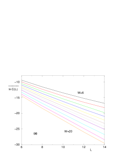
We show on Fig. 6 (a) the decay with the distance $L$ of the disorder-average $\overline{\ln C(L)}$ for various disorder strengths in the range $6\leq W\leq 20$ : these curves correspond to an exponential decay with $L$ of the typical value $C_{L}^{typ}\equiv e^{\overline{\ln C(L)}}$

$$\ln(C_{L}^{typ})\equiv\overline{\ln C_{L}(W>W_{c})}\ \mathop{\simeq}_{L\to\infty}-\frac{L}{\xi_{C}(W)}$$ (30)

where $\xi_{C}$ represents the correlation length that diverges at the delocalization transition

$$\xi_{C}(W)\mathop{\simeq}_{W\to W_{c}^{+}}(cst)(W-W_{c})^{-\nu_{C}}$$ (31)

We show on Fig. 6 (b) our numerical result for the slope $1/\xi_{C}(W)$ as a function of the disorder strength $W$ in the region $6\leq W\leq 20$, as compared to $1/\xi_{loc}(W)$ found previously for the renormalized hopping in configuration space (see Eq. 12 and Fig. 2). Our conclusion is that up to a numerical prefactor, these two correlation lengths seen either in the renormalized hoppings in configuration space, or in the two-point correlation function in real space, contain essentially the same information. In particular, a three-parameter fit of the form of Eq. 31 yields values for the critical point $W_{c}$ and for the critical exponent $\nu_{C}\sim\nu_{loc}$ that are compatible with the values estimated previously from the data in configuration space.

In the delocalized phase however, it is not clear to us what are the theoretical expectations for the decay in $L$ of the two-point correlation function of Eq. 29, and our numerical data are not sufficiently clear by themselves to indicate which procedure should be used to fit the data in order to obtain information on the critical behavior in the delocalized phase. Further work is needed to clarify this point, or to find other real-space observables that display a clearer behavior in the delocalized phase.

To summarize this section, our numerical data concerning the real-space two-point correlation function of Eq. 29 indicate that the correlation length measured previously in configuration space is essentially equivalent to the correlation length measured in real space. In particular, this shows that the results obtained in configuration space do not depend to much on the particular choice (c2) of alternate configurations made in section II.3.

VI Conclusion

In this paper, we have proposed to study many-body localization transition via an exact renormalization procedure in configuration space that generalizes the Aoki real-space RG procedure for Anderson localization one-particle models. For the one-dimensional lattice model of interacting fermions with disorder studied previously by Oganesyan and Huse [26], we have studied numerically the statistical properties of the renormalized hopping $V_{L}$ between two configurations separated by a distance $L$ in configuration space. Our numerical results are compatible with the existence of a many-body localization transition at a finite disorder strength of order $W_{c}\sim 5.6$. In the localized phase $W>W_{c}$, we have found that the typical renormalized hopping $V_{L}^{typ}\equiv e^{\overline{\ln V_{L}}}$ decays exponentially in $L$ as $(\ln V_{L}^{typ})\simeq-\frac{L}{\xi_{loc}}$ and that the localization length diverges as $\xi_{loc}\sim(W-W_{c})^{-\nu_{loc}}$ with the critical exponent of order $\nu_{loc}\simeq 0.45$. In the delocalized phase $W<W_{c}$, we have found that the renormalized hopping $V_{L}$ remains a finite random variable $V_{\infty}$ as $L\to\infty$, and that the typical asymptotic value $V_{\infty}^{typ}\equiv e^{\overline{\ln V_{\infty}}}$ presents an essential singularity $(\ln V_{\infty}^{typ})\sim-(W_{c}-W)^{-\kappa}$ with an exponent of order $\kappa\sim 1.4$. We have argued that the analogy with Anderson localization on the Cayley tree is important as an example of Anderson transition on a space of infinite dimension (in the sense of Eq. 21) that presents essential singularities and that it suggests a specific form of finite size scaling that we have tested. Even if the numerical values of the exponents are not expected to be precise, as a consequence of the limited system sizes studied $L\leq 14$, we hope that the scaling laws that emerge are valid. Of course, it would be very useful in the future to test these results with other numerical methods like the Density Matrix Renormalization Group method, that allow to study these interacting one-dimensional models for much bigger system sizes [34, 35, 36, 37]. Finally, we have shown that the present analysis in configuration space is compatible with the localization properties displayed by the simplest two-point correlation function in real space.

In conclusion, the reformulation of many-body localization problems as Anderson localization models in configuration space raises the question of Anderson localization on specific networks (see [48] and references therein), that are completely different from the regular lattices that have been considered in the field of one-particle models. For a many-body problem defined on a domain of size $L^{d}$, the number of configurations (i.e. the nodes of the network) grows exponentially ${\cal N}_{L}\propto e^{(cst)L^{d}}$. Each configuration has a different connectivity in this space of configurations, but it is typically of order $L^{d}$ (assuming a finite density of fermions, with a finite number of short-range hopping for each fermion). Besides the interest in specific many-body models, an important issue is of course to understand which properties of this complex network are relevant to determine the universality class of the corresponding Anderson transition.

VII Acknowledgements

It is a pleasure to thank D.A. Huse, A.D. Mirlin, T. Prosen and M. Znidaric for useful discussions and correspondence. After this work was completed, we became aware of the work [49] that suggests an infinitite-randomness scaling for the many-body localization transition of a quantum spin chain.

References

- [1] P.W. Anderson, Phys. Rev. 109, 1492 (1958).
- [2] M. Janssen, Phys. Rep. 295, 1 (1998).
- [3] P. Markos, Acta Physica Slovaca 56, 561 (2006).
- [4] F. Evers and A.D. Mirlin, Rev. Mod. Phys. 80, 1355 (2008).
- [5] D. Belitz and T. R. Kirkpatrick, Rev. Mod. Phys. 66, 261 (1994).
- [6] A.L. Efros and B.I. Shklovskii, J. Phys. C 8, L49 (1975).
- [7] M. Muller and L. B. Ioffe, Phys. Rev. Lett. 93, 256403 (2004)
- [8] M. Goethe and M. Palassini, Phys. Rev. Lett. 103, 045702 (2009).
- [9] T. Vojta, F. Epperlein and M. Schreiber, Phys. Rev. Lett 81, 4212 (1998).
- [10] R. Berkovits, J.W. Kantelhardt, Y. Avishai, S. Havlin and A. Bunde, Phys. Rev. B 63, 085102 (2001); R. Berkovits and J.W. Kantelhardt, Phys. Rev. B 65, 125308 (2002)
- [11] G. Fleury and X. Waintal, Phys. Rev. Lett. 100, 076602 (2008) and Phys. Rev. Lett. 101, 226803 (2008).
- [12] T. Giamarchi and H. Schulz, Europhys. Lett. 3, 1287 (1987) and Phys. Rev. B 37, 325 (1988).
- [13] M.P.A. Fisher, P.B. Weichman, G. Grinstein, and D.S. Fisher, Phys. Rev. B 40, 546 (1989).
- [14] E. Altman, Y. Kafri, A. Polkovnikov and G. Refael, Phys. Rev. Lett. 100, 170402 (2008) and arXiv:0909.4096.
- [15] G.M. Falco, T. Nattermann, V.L. Pokrovsky, Europhys. Lett. 85, 30002 (2009) and G.M. Falco, T. Nattermann, V.L. Pokrovsky, Phys. Rev B 80, 104515 (2009).
- [16] L. Ioffe and M. Mézard, arxiv : 0909.2263; M. Müller, arxiv:0909.2260.
- [17] I.L. Aleiner, B.L. Altshuler and G. V. Shlyapnikov, arxiv: 0910:4534.
- [18] B.L. Altshuler, Y. Gefen, A. Kamenev and L.S. Levitov, Phys. Rev. Lett. 78, 2803 (1997).
- [19] R. Berkovits and Y. Avishai, Phys. Rev. Lett. 80, 568 (1998).
- [20] X. Leyronas, J. Tworrzydlo and C.W.J. Beenakker, Phys. Rev. Lett. 82, 4894 (1999) ; X. Leyronas, P.G. Silvestrov and C.W.J. Beenakker, Phys. Rev. Lett. 84, 3414 (2000).
- [21] P.G. Silvestrov, Phys. Rev. B 64, 113309 (2001).
- [22] V.V. Flambaum and F. M. Izrailev, Phys. Rev. E 64, 036220 (2001).
- [23] R. Berkovits1, Y. Gefen, Igor V. Lerner, and B. L. Altshuler , Phys. Rev. B 68, 085314 (2003).
- [24] I.V. Gornyi, A.D. Mirlin and D.G. Polyakov, Phys. Rev. Lett. 95, 206603 (2005).
- [25] D.M. Basko, I.L. Aleiner, B.L. Altshuler, Annals of Physics 321, 1126 (2006) and Phys. Rev. B 76, 052203 (2007).
- [26] V. Oganesyan and D.A. Huse, Phys. Rev. B 75, 155111 (2007).
- [27] H. Aoki, J. Phys. C 13, 3369 (1980).
- [28] H. Aoki, Physica A 114, 538 (1982).
- [29] H. Kamimura and H. Aoki, “The physics of interacting electrons and disordered systems”, Clarendon Press Oxford (1989).
- [30] C.J. Lambert and D. Weaire, phys. stat. sol. (b) 101, 591 (1980).
- [31] C. Monthus and T. Garel, Phys. Rev. B 79, 205120 (2009)
- [32] C. Monthus and T. Garel, Phys. Rev. B 80, 024203 (2009).
- [33] M. Leadbeater, R.A, Römer and M. Schreiber, Eur. Phys. J B 8, 643 (1999).
- [34] P. Schmitteckert, T. Schulze, C. Schuster, P. Schwab, and U. Eckern, Phys. Rev. Lett. 80, 560 (1998); P. Schmitteckert, R. A. Jalabert, D. Weinmann, and J.-L. Pichard, Phys. Rev. Lett. 81, 2308 (1998); P. Schmitteckert and R. Werner,Phys. Rev. B 69, 195115 (2004).
- [35] R. A. Molina, D. Weinmann, R. A. Jalabert, G.-L. Ingold, and J.-L. Pichard, Phys. Rev. B 67, 235306 (2003); R. A. Molina, P. Schmitteckert, D. Weinmann, R. A. Jalabert, G.-L. Ingold and J.-L. Pichard, EPJB 39, 107 (2004).
- [36] J. M. Carter and A. MacKinnon Phys. Rev. B 72, 024208 (2005); A. MacKinnon Pramana 70, 211 (2008).
- [37] M. Znidaric, T. Prosen and P. Prelovsek, Phys. Rev. B 77, 064426 (2008).
- [38] S. Mukerjee, V. Oganesyan and D.A. Huse, Phys. Rev. B 73, 035113 (2006).
- [39] R. Abou-Chacra, P.W. Anderson and D.J. Thouless, J. Phys. C : Solid State Physics 6, 1734 (1973) ( see also R. Abou-Chacra and D. J. Thouless, J. Phys. C: Solid State Phys. 7, 65 (1974) ).
- [40] H. Kunz and B. Souillard, J. Physique Lettres 44, L411 (1983).
- [41] A.D. Mirlin and Y.V. Fyodorov, Nucl. Phys. B 366, 507 (1991).
- [42] K.B. Efetov, “Supersymmetry in disorder and chaos”, Cambridge University Press (1997).
- [43] B. Derrida and G.J. Rodgers, J. Phys. A : Math. Gen. 26, L457 (1993).
- [44] J.D. Miller and B. Derrida, J. Stat. Phys. 75, 357 (1994).
- [45] C. Monthus and T. Garel, J. Phys. A Math Theor 42, 075002 (2009).
- [46] A.D. Mirlin and Y.V. Fyodorov, Phys. Rev. Lett. 72, 526 (1994).
- [47] B. Derrida and D. Simon, EPL 78, 60006 (2007); D. Simon and B. Derrida, J. Stat. Phys. 131, 203 (2008); D. Simon, PhD Thesis (2008), available at http://tel.archives-ouvertes.fr/tel-00286612/fr/
- [48] R. Berkovits, Eur. Phys. J. Special Topics 161, 259 (2008).
- [49] A. Pal and D.A. Huse, arxiv:1003.2613