Linear Scaling Solution of the Time-Dependent Self-Consistent-Field Equations
Abstract
A new approach to solving the Time-Dependent Self-Consistent-Field equations is developed based on the double quotient formulation of Tsiper [J. Phys. B, 34 L401 (2001)]. Dual channel, quasi-independent non-linear optimization of these quotients is found to yield convergence rates approaching those of the best case (single channel) Tamm-Dancoff approximation. This formulation is variational with respect to matrix truncation, admitting linear scaling solution of the matrix-eigenvalue problem, which is demonstrated for bulk excitons in the polyphenylene vinylene oligomer and the (4,3) carbon nanotube segment.
The Time-Dependent Self-Consistent-Field equations together with models that include some portion of the Hartree-Fock (HF) exchange admit control over the range of self-interaction in the optical response Autschbach (2009); Song et al. (2009); Igumenshchev et al. (2007); Magyar and Tretiak (2007), and are related to new models of electron correlation based on the Random Phase Approximation (RPA) Lu et al. (2009); Furche (2008); Harl and Kresse (2009); Toulouse et al. (2009). Solving the TD-SCF equations is challenging due to an unconventional J-symmetric structure of the naive molecular orbital (MO) representation,
| (1) |
where and are Hermitian blocks corresponding to order tensors spanning transitions between occupied and virtual sub-spaces, is the real excitation energy and is the corresponding transition density. By construction, the MO representation allows strict separation between the dyadic particle-hole (ph) and hole-particle (hp) solutions, and , for which specialized algorithms exist. Nevertheless, convergence of the naive -symmetric problem is typically much slower than the corresponding Hermitian Tamm-Dancoff approximation (TDA), , which is of reduced dimensionality in the MO representation.
Several TD-SCF eigensolvers are based on the oscillator picture with and the Hermitian potential and kinetic matrices, and the dual corresponding to position and momentum. This picture avoids the imbalance whilst admitting conventional solutions based on the Hermitian matrix as shown by Tamara and Udagawa Tamura and Udagawa (1964) and extended by Narita and Shibuya with second order optimization of the quotient Narita and Shibuya (1992). More recently, Tsiper considered the quotients
| (2) |
and developed a corresponding dual channel Lanczos solver. Subspace solvers in this dual representation have recently been surveyed by Tretiak, Isborne, Niklasson and Challacombe (TINC) Tretiak et al. (2009), with comparative results for semi-empirical models.
Another challenge is dimensionality and scaling. Writing Eq. (1) in the general form , admitting arbitrary representation, the superoperator matrix is a tetradic, with N the number of basis functions, assumed proportional to system size. In practice the action of onto is carried out implicitly as using an existing framework for construction of the effective Hamiltonian (Fockian) , where is the one-particle reduced density matrix, is a screening operator involving Coulomb, exchange and/or exchange-correlation terms and the correspondence between superoperator and functional notation is given by a tensorial mapping between diadic and matrix, .
Recent efforts have focused on addressing the problem of dimensionality by employing linear scaling methods that reduce the cost of within Density Functional Theory (DFT) to . However, this remains an open problem for the Hartree-Fock (HF) exchange, an ingredient in models that account for charge transfer in the dynamic and static response, including the Random Phase Approximation (RPA) at the pure HF level of theory. Likewise, scaling of the TD-SCF eigenproblem remains formidable due to associated costs of linear algebra, even when using powerful Krylov subspace methods. Underscoring this challenge, one of the most successful approaches to linear scaling TD-DFT avoids the matrix eigenproblem entirely through explicit time-evolution Yokojima and Chen (1999); Yam et al. (2003).
Linear scaling matrix methods exploit quantum locality, manifest in approximate exponential decay of matrix elements expressed in a well posed, local basis; with the dropping of small elements below a threshold, , this decay leads to sparse matrices and complexity at the forfeit of full precision Challacombe (1999, 2000); Niklasson et al. (2003). Likewise, linear scaling methods for computing the HF exchange employ an advanced form of direct SCF, exploiting this decay in the rigorous screening of small exchange interactions bellow the two-electron integral threshold Schwegler et al. (1997). The consequence of these linear scaling approximations is an inexact linear algebra that challenges Krylov solvers due to nested error accumulation, a subject of recent formal interest Simoncini (2005); Simoncini and Szyld (2007). Consistent with this view, TINC found that matrix perturbation (a truncation proxy) disrupts convergence of Krylov solvers with slow convergence, i.e. Lanczos and Arnoldi for the RPA, but has less impact on solvers with rapid convergence, i.e. generically for the TDA or Davidson for the RPA. Relative to semi-empirical Hamiltonians, the impact of incompleteness on subspace iteration may be amplified with first principles models and large basis sets (ill-conditioning).
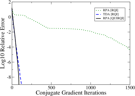
An alternative is Rayleigh Quotient Iteration (RQI), which poses the eigenproblem as non-linear optimization and is variational with respect to matrix perturbation. Narita and Shibuya Narita and Shibuya (1992) considered optimization of the quotient with second order methods, but these are beyond the capabilities of current linear scaling technologies and also, convergence is disadvantaged by a power of . For semi-empirical Hamiltonians, TINC found that optimization of the Thouless functional corresponding to the solution of Eq. (1), was significantly slower for the RPA relative to the TDA, and also compared to subspace solvers. For first principles models and non-trivial basis sets, this naive RQI can become pathologically slow as shown in Fig. 1. On the other hand, the Tsiper formulation exposes the underlying pseudo-Hermitian structure of the TD-SCF equations. Here, this structure is exploited with QUasi-Independent Rayleigh Quotient Iteration (QUIRQI), involving dual channel optimization of the Tsiper quotients coupled only weakly through line search.

Our development begins with a brief review of the representation independent formulation developed by TINC, which avoids the cost of rotating into an explicit p-h, h-p symmetry. Instead, this symmetry is maintained implicitly via annihilation, , with the first order reduced density matrix and its compliment. Likewise, the indefinite metric associated with the -symmetry of Eq. (1) is carried through the generalized norm . Introducing the operator equivalents, and , the Tsiper functional becomes Transformations between the transition density and the dual space involves simple manipulations and minimal cost, allowing Fock builds with the transition density and optimization in the dual space. The splitting operation is given by and . Likewise, and . The back transformation (merge) from dual to density is . This framework provides the freedom to work in any orthogonal representation, and to switch between transition density and oscillator duals with minimal cost.
QUIRQI is given in Algorithm 1. It begins with a guess for the transition density, which is then split into its dual (lines 2-3). The choice of initial guess is discussed later. Lines 4-24 consist of the non-linear conjugate gradient optimization of the nearly independent channels: In each step, the flow of information proceeds from optimization of the duals to builds involving the density and back to the duals in a merge-annihilate-truncate-build-split-truncate (MATBST) sequence. For the variables , and this sequence is comprised by lines 22-23 and 5-7, and lines 15-19 for the corresponding conjugate gradients , and . Truncation is carried out with the filter operation as described in Ref. Niklasson et al. (2003), with cost and error determined by the matrix threshold .
The Tsiper functional is the sum of dual quotients and , determined at line 8, followed by the gradients and computed at line 9. After the first cycle, the corresponding relative error (10) and maximum matrix element of the gradient (11) are computed and used as an exit criterion at line 4, along with non-variational behavior
Next, the Polak-Ribiere variant of non-linear conjugate gradients yields the search direction in each channel, and (12-14). The action of on to and is then computed, again with a MATBST sequence (15-19), followed by a self-consistent dual channel line search at line 20, as described below. With steps and in hand, minimizing updates are taken along each conjugate direction (22), and the cycle repeats with the MATBST sequence spanning lines 21-23 and 5-7.
Optimization of the Tsipper functional involves a two dimensional line-search (line 20) corresponding to minimization of
| (3) |
with coupling entering through terms in the denominator such as . A minimum in Eq. (3) can be found quickly to high precision by alternately substituting one-dimensional solutions one into the other until self-consistency is reached. This semi-analytic approach starts with a rough guess at the pair (eg. found by a coarse scan) followed by iterative substitution, where for example the -channel update is
| (4) | |||
with an analogous update for the -channel obtained by swapping subscripts. As the solution decouples ( and become small) the steps are found independently.
QUIRQI has been implemented in FreeON Bock et al. (2009), which employs the linear scaling Coulomb and Hartree-Fock exchange kernels QCTC and ONX with cost and accuracy controlled by the two-electron screening threshold Schwegler et al. (1997). N-scaling solution of the QUIRQI matrix equations is achieved with the sparse approximate matrix-matrix multiply (SpAMM), with cost and accuracy determined by the drop tolerance Challacombe (1999, 2000); Niklasson et al. (2003). All calculations were carried out with version 4.3 of the gcc/gfortran compiler under version 8.04 of the Ubuntu Linux distribution and run on a fully loaded 2GHz AMD Quad Opteron 8350.
For systems studied to date, QUIRQI is found to converge monotonically with rates comparable to the TDA as shown in Fig. 1. Based on the comparative performance presented by TINC, the TDA rate of convergence appears to be a lower bound for RPA solvers. In addition to the convergence rate, performance is strongly determined by the initial guess. The following results have been obtained using the polarization response density along the polymer axis Tretiak et al. (2009), which can be computed in by Perturbed Projection Weber et al. (2004). Also, a relative precision of 4 digits in the excitation energy is targeted with the convergence parameters and , with exit from the optimization loop on violation of monotonic convergence ( due to precision limitations associated with linear scaling approximations).
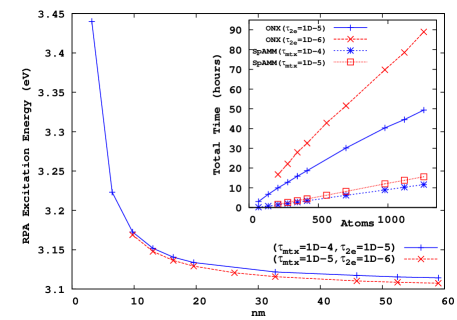
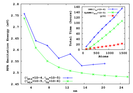
In Fig. 2, linear scaling and convergence to the bulk limit are demonstrated for a series of polyphenylene vinylene (PPV) oligomers at the RHF/6-31G** level of theory for the threshold combinations and . Significantly more conservative thresholds have been used for the Coulomb sums, which incur only minor cost. Convergence is reached in iterations, with the cost of Coulomb summation via QCTC comparable to the cost of SpAMM(). In Fig. 3, linear scaling and convergence to the bulk limit are demonstrated for a series of (4,3) carbon nanotube segments at the RHF/3-21G level of theory for the same threshold combinations, again with convergence achieved in about 24-25 cycles. In both cases, tightening the pair leads to a systematically improved result. While the thresholds that work well for PPV lead to a non-monotone behavior with respect to extent for the nanotube series, dropping one more decade to leads to a sharply improved behavior. Dropping thresholds further to yields identical results to within the convergence criteria ( four digits) across the series, also scaling with but at roughly twice the cost.
These results demonstrate that QUIRQI can achieve both systematic error control and linear scaling in solution of the RPA eigenproblem for systems with extended conjugation. Relative to PPV, the greater numerical sensitivity encountered with the nanotube series is consistent with the ground state problem, where a smaller band gap and greater atomic connectivity typically demand tighter thresholds.
QUIRQI exploits decoupling of the Tsipper functional into nearly independent, pseudo-Hermitian quotients leading to aggressive convergence rates equivalent to the fully Hermitian TDA, while remaining variational with respect to matrix truncation (). However, QUIRQI is not variational with respect to the screening parameter . It can be systematically improved by tightening though, due to rigorous error bounds based on the Schwartz inequality Schwegler et al. (1997). These properties present opportunities for more precise error control as suggested by Rubensson, Rudberg and Salek Rubensson et al. (2008). Further, these properties are expected to hold even for the most general SCF models, with the only difference being an increasingly localized transition density matrix and larger cost prefactor with an increasing DFT component. Finally, a variational approach allows considerable flexibility in the path to solution, as errors due to approximation can be overcome by optimization, offering opportunities for single precision GPU acceleration, variable thresholding, incremental Fock builds as well as extrapolation techniques.


This work was supported by the U.S. Department of Energy and Los Alamos LDRD funds. Los Alamos National Laboratory was operated by the Los Alamos National Security, LLC, for the National Nuclear Security Administration of the U.S. Department of Energy under Contract No. DE-AC52-06NA25396. Special acknowledgments go the International Ten Bar Café for scientific vlibations, and to Sergei Tretiak and Nicolas Bock for valuable input.
References
- Autschbach (2009) Autschbach, J., 2009, Chem. Phys. Chem. 10, 1757.
- Bock et al. (2009) Bock, N., M. Challacombe, C. K. Gan, G. Henkelman, K. Nemeth, A. M. N. Niklasson, A. Odell, E. Schwegler, C. J. Tymczak, and V. Weber, 2009, FreeON ( Sep-18-2009 ), Los Alamos National Laboratory (LA-CC-04-086, Copyright University of California)., URL http://www.nongnu.org/freeon/.
- Challacombe (1999) Challacombe, M., 1999, J. Chem. Phys. 110, 2332.
- Challacombe (2000) Challacombe, M., 2000, Comp. Phys. Comm. 128, 93.
- Furche (2008) Furche, F., 2008, J. Chem. Phys. 129(11), 114105.
- Harl and Kresse (2009) Harl, J., and G. Kresse, 2009, Phys. Rev. Lett. 103(5), 056401.
- Igumenshchev et al. (2007) Igumenshchev, K. I., S. Tretiak, and V. Y. Chernyak, 2007, J. Chem. Phys. 127(11), 114902.
- Lu et al. (2009) Lu, D., Y. Li, D. Rocca, and G. Galli, 2009, Phys. Rev. Lett. 102(20), 206411.
- Magyar and Tretiak (2007) Magyar, R. J., and S. Tretiak, 2007, J. Chem. Theor. Comp. 3, 976.
- Narita and Shibuya (1992) Narita, S., and T. Shibuya, 1992, Can. J. Chem. 70, 296.
- Niklasson et al. (2003) Niklasson, A. M. N., C. J. Tymczak, and M. Challacombe, 2003, J. Chem. Phys. 118, 8611.
- Rubensson et al. (2008) Rubensson, E. H., E. Rudberg, and P. Salek, 2008, J. Math. Phys. 49(3), 032103.
- Schwegler et al. (1997) Schwegler, E., M. Challacombe, and M. Head-Gordon, 1997, J. Chem. Phys. 106, 9708.
- Simoncini (2005) Simoncini, V., 2005, SIAM J. Num. Anal. 43(3), 1155 .
- Simoncini and Szyld (2007) Simoncini, V., and D. B. Szyld, 2007, Num. Lin. Alg. App. 14(1), 1 .
- Song et al. (2009) Song, J.-W., M. A. Watson, and K. Hirao, 2009, J. Chem. Phys. 131(14), 144108.
- Tamura and Udagawa (1964) Tamura, T., and T. Udagawa, 1964, Nuc. Phys. 53, 33.
- Toulouse et al. (2009) Toulouse, J., I. C. Gerber, G. Jansen, A. Savin, and J. G. Ángyán, 2009, Phys. Rev. Lett. 102(9), 096404.
- Tretiak et al. (2009) Tretiak, S., C. M. Isborn, A. M. N. Niklasson, and M. Challacombe, 2009, J. Chem. Phys. 130(5), 054111.
- Weber et al. (2004) Weber, V., A. M. N. Niklasson, and M. Challacombe, 2004, Phys. Rev. Lett. 92, 193002.
- Yam et al. (2003) Yam, C. Y., S. Yokojima, and G. Chen, 2003, J. Chem. Phys. 119(17), 8794.
- Yokojima and Chen (1999) Yokojima, S., and G. H. Chen, 1999, Chem. Phys. Lett. 300(5-6), 540.