Scattering and transport statistics at the metal-insulator transition: A numerical study of the power-law banded random matrix model

Abstract

We study numerically scattering and transport statistical properties of the one-dimensional Anderson model at the metal-insulator transition described by the Power-law Banded Random Matrix (PBRM) model at criticality. Within a scattering approach to electronic transport, we concentrate on the case of a small number of single-channel attached leads. We observe a smooth crossover from localized to delocalized behavior in the average scattering matrix elements, the conductance probability distribution, the variance of the conductance, and the shot noise power by varying $b$ (the effective bandwidth of the PBRM model) from small ($b\ll 1$) to large ($b>1$) values. We contrast our results with analytic random matrix theory predictions which are expected to be recovered in the limit $b\to\infty$. We also compare our results for the PBRM model with those for the three-dimensional (3D) Anderson model at criticality, finding that the PBRM model with $b\in[0.2,0.4]$ reproduces well the scattering and transport properties of the 3D Anderson model.

I Introduction

The study of systems at the Anderson metal-insulator transition (MIT) has been a subject of intensive research activity for several decades. A58 ; AMPJ95 ; AKL91 ; EM08 In particular, much interest has been focused on the scattering properties of critical systems by analysing the probability distribution functions of the resonance widths $\Gamma$ and Wigner delay times $\tau_{\mbox{\tiny W}}$, MK05 ; OF05 ; MFME06 ; OKG03 ; F03 ; TC99 ; KW02 ; KW02b ; WMK06 ; MI06 as well as the transmission or dimensionless conductance $T$. S90 ; M94 ; M99 ; SO97 ; SOK00 ; SMO00 ; WLS98 ; RS01 ; RMS001 ; TM02 ; SM05 ; JMZ99 The distribution functions of $\Gamma$ and $\tau_{\mbox{\tiny W}}$ have been shown to be related to the properties of the corresponding closed systems, i.e., the fractality of the eigenstates and the critical features of the MIT. On the other hand, at the MIT, the distribution of conductances $w(T)$ has been found to be universal, i.e., size independent, but dependent on the adopted model, dimensionality, symmetry, and even boundary conditions of the system. $w(T)$ has been studied for systems in two and more dimensions with a large number of attached single-channel leads. S90 ; M94 ; M99 ; SO97 ; SOK00 ; SMO00 ; WLS98 ; RS01 ; RMS001 ; TM02 ; SM05 ; JMZ99 In fact, concerning the conductance of one-dimensional (1D) systems and its statistical distribution, the regime of small number of leads has been left almost unexplored. JMZ99 ; SZ02 ; MG09a ; MG09b

In the present work we study numerically several statistical properties of the scattering matrix and the electronic transport across disordered systems in one and three dimensions described by the Power-law Banded Random Matrix (PBRM) model at criticality and the three-dimensional (3D) Anderson model at the MIT, respectively. We stress that we concentrate on the case of a small number of attached leads each of them supporting one open channel.

The organization of this paper is as follows. In the next subsection we define the PBRM model, the 3D Anderson model, as well as the scattering setup. We also define the scattering quantities under investigation and provide the corresponding analytical predictions from random scattering-matrix theory (RMT) for systems with time-reversal symmetry. These analytical results will be used as a reference along the paper. In Section II we analyse the average scattering matrix elements, the conductance probability distribution, the variance of the conductance, and the shot noise power for the PBRM model as a function of its effective bandwidth $b$. In Section III we compare the results of the PBRM model at criticality with the scattering and transport properties of the 3D Anderson model. Finally, Section IV is left for conclusions.

I.1 The PBRM and the 3D Anderson models

As we have mentioned above, in the present study we adopt two models, namely, the PBRM model at criticality and the 3D Anderson model at the MIT.

The PBRM model EM08 ; MFDQS96 describes 1D samples of length $L$ with random long-range hopping. This model is represented by $N\times N$ ($N=L$) real symmetric matrices whose elements are statistically independent random variables drawn from a normal distribution with zero mean, $\langle H_{ij}\rangle=0$, and a variance decaying as a power law $\langle|H_{ij}|^{2}\rangle\sim(b/|i-j|)^{2\alpha}$, where $b$ and $\alpha$ are parameters. There are two prescriptions for the variance of the PBRM model: the so-called non-periodic,

$$\langle|H_{ij}|^{2}\rangle=\frac{1}{2}\frac{1+\delta_{ij}}{1+\left(|i-j|/b\right)^{2\alpha}}\ ,$$ (1)

where the 1D sample is in a line geometry; and the periodic,

$$\langle|H_{ij}|^{2}\rangle=\frac{1}{2}\frac{1+\delta_{ij}}{1+\left[\sin\left(\pi|i-j|/L\right)/(\pi b/L)\right]^{2\alpha}}\ ,$$ (2)

where the sample is in a ring geometry. Field-theoretical considerations EM08 ; MFDQS96 ; KT00 and detailed numerical investigations EM08 ; EM00b ; V03 have verified that the PBRM model undergoes a transition at $\alpha=1$ from localized states for $\alpha>1$ to delocalized states for $\alpha<1$. This transition shows all the key features of the Anderson MIT, including multifractality of eigenfunctions and non-trivial spectral statistics at the critical point. Thus the PBRM model possesses a line of critical points $b\in(0,\infty)$. We set $\alpha=1$ in our study, i.e., we work with the PBRM model at criticality.

The 3D Anderson model with diagonal disorder is described by the tight-binding Hamiltonian (TBH)

$$H=\sum_{\bf n}|{\bf n}\rangle W_{\bf n}\langle{\bf n}|+\sum_{{\bf(n,m)}}|{\bf n}\rangle\langle{\bf m}|\ ,$$ (3)

where ${\bf n}\equiv(n_{x},n_{y},n_{z})$ labels all the $N=L^{3}$ sites of a cubic lattice with linear size $L$, while the second sum is taken over all nearest-neighbour pairs ${\bf(n,m)}$ on the lattice. The on-site potentials $W_{\bf n}$ for $1\leq n_{x},n_{y},n_{z}\leq L$ are independent random variables. When $W_{\bf n}$ are Gaussian distributed, with zero mean and variance $W^{2}/12$, the MIT at energy $E\simeq 0$ occurs for $W=W_{c}\simeq 21.3$. See Refs. [M99, ; RMS01, ; MW99, ]. Then, for $W<W_{c}$ ($W>W_{c}$) the system is in the metallic (insulating) regime. We set $W=W_{c}$ in our study.

We open the isolated samples, defined above by the PBRM model and the 3D Anderson model, by attaching $2M$ semi-infinite single channel leads. Each lead is described by the 1D semi-infinite TBH

$$H_{\mbox{\tiny lead}}=\sum^{-\infty}_{n=1}(|n\rangle\langle n+1|+|n+1\rangle\langle n|)\ .$$ (4)

Using standard methods MW69 one can write the scattering matrix ($S$-matrix) in the form SOKG00 ; KW02

$$S(E)=\left(\begin{array}[]{cc}r&t^{\prime}\\ t&r^{\prime}\end{array}\right)={\bf 1}-2i\sin(k)\,{\cal W}^{\,T}(E-{\cal H}_{\rm eff})^{-1}{\cal W}\ ,$$ (5)

where ${\bf 1}$ is the $2M\times 2M$ unit matrix, $k=\arccos(E/2)$ is the wave vector supported in the leads, and ${\cal H}_{\rm eff}$ is an effective non-hermitian Hamiltonian given by

$${\mathcal{H}}_{\rm eff}=H-e^{ik}{\cal W}{\cal W}^{\,T}\ .$$ (6)

Here, ${\cal W}$ is an $N\times 2M$ matrix that specifies the positions of the attached leads to the sample. Its elements are equal to zero or $\epsilon$, where $\epsilon$ is the coupling strength. Moreover, assuming that the wave vector $k$ do not change significantly in the centre of the band, we set $E=0$ and neglect the energy dependence of ${\mathcal{H}}_{\rm eff}$ and $S$.

I.2 RMT predictions for the Circular Orthogonal Ensemble

Notice from Eqs. (1-2) that in the limit $b\to\infty$ the PBRM model reproduces the Gaussian Orthogonal Ensemble. Therefore, in that limit we expect the statistics of the scattering matrix, Eq. (5), to be determined by the Circular Orthogonal Ensemble (COE) which is the appropriate ensemble for systems with time reversal symmetry. Thus, below, we provide the statistical results for the average $S$-matrix and the transport quantities to be analysed in the following sections, assuming the orthogonal symmetry. In all cases, we also assume the absence of direct processes, i.e., $\langle S\rangle=0$.

We start with the average of the $S$-matrix elements. It is known that

$$\left\langle|S_{aa^{\prime}}|^{2}\right\rangle_{\mbox{\tiny COE}}=\frac{1+\delta_{aa^{\prime}}}{2M+1}\ ,$$ (7)

where $\left\langle\cdot\right\rangle$ means ensemble average over the COE.

Within a scattering approach to the electronic transport, once the scattering matrix is known one can compute the dimensionless conductance $T={\mbox{Tr}}(tt^{\dagger})$ and its distribution $w(T)$. For $M=1$, i.e., considering two single-channels leads attached to the sample, $w(T)$ is given by

$$w(T)_{\mbox{\tiny COE}}=\frac{1}{2\sqrt{T}}\ ,$$ (8)

while for $M=2$,

$$w(T)_{\mbox{\tiny COE}}=\left\{\begin{array}[]{ll}\frac{3}{2}T\ ,&0<T<1\\ \frac{3}{2}\left(T-2\sqrt{T-1}\right)\ ,&1<T<2\\ \end{array}\right.\ .\\$$ (9)

For arbitrary $M$, the predictions for the average value of $T$ and its variance are

$$\left\langle T\right\rangle_{\mbox{\tiny COE}}=\frac{M}{2}-\frac{M}{2(2M+1)}\$$ (10)

and

$$\mbox{var}(T)_{\mbox{\tiny COE}}=\frac{M(M+1)^{2}}{(2M+1)^{2}(2M+3)}\ ,$$ (11)

respectively. For the derivation of the expressions above see for example Ref. [MK04, ]. Another transport quantity of interest is the shot noise power $P=\left\langle{\mbox{Tr}}(tt^{\dagger}-tt^{\dagger}tt^{\dagger})\right\rangle$, which as a function of $M$ reads evgeny ; HMBH06 ; savin

$$P_{\mbox{\tiny COE}}=\frac{M(M+1)^{2}}{2(2M+1)(2M+3)}\ .$$ (12)

In the following sections we focus on $\left\langle|S_{aa^{\prime}}|^{2}\right\rangle$, $\left\langle T\right\rangle$, $\mbox{var}(T)$, and $P$ for the PBRM model and the 3D Anderson model, both at the MIT. In all cases we set the coupling strength $\epsilon$ such that $\left\langle S\right\rangle\approx 0$ in order to compare our results, in the proper limits, with the RMT predictions introduced above.

II PBRM model

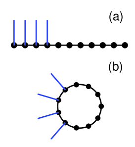
We attach the $2M$ leads to the first $2M$ sites of the 1D sample described by the PBRM model. That is, in the non-periodic version of the PBRM model, Eq. (1), we attach the leads at the boundary of the system. See Fig. 1(a). While in the periodic version, Eq. (2), we attach them to the bulk. See Fig. 1(b). In the latter case, finite size effects are considerably reduced. However, the quantities we analyse below are $L$-independent once $L$ is much larger than the number of attached leads for both versions of the PBRM model.

We point out that our setup is significantly different from the one used in Refs. [MG09a, ; MG09b, ], where the conductance has also been studied using the PBRM model. There, for example, the leads in the $M=1$ case are attached to sites which are separated a distance of $L/2$ and $L$ in the periodic and non-periodic versions of the PBRM model, respectively. In such situation the scattering quantities are strongly $L$-dependent.

Figure 1: (Color online) Scattering setup. $2M$ leads, shown as blue (gray) lines, are attached to $2M$ sites (black dots) of a 1D sample described by the (a) non-periodic and (b) periodic versions of the PBRM model. The case $M=2$ with $L=11$ is shown as example.

Figure 2: (Color online) Black [red (gray)] symbols: Average $S$-matrix elements $\left\langle|S_{11}|^{2}\right\rangle$ and $\left\langle|S_{12}|^{2}\right\rangle$ for the periodic [non-periodic] PBRM model at criticality as a function of (a) $b$ and (b) $D_{2}$ for $M=1$. The blue (gray) dot-dashed lines correspond to 2/3 and 1/3; the RMT prediction for $\left\langle|S_{11}|^{2}\right\rangle$ and $\left\langle|S_{12}|^{2}\right\rangle$, respectively, given by Eq. (7). The black [red (gray)] dashed lines in (a) are Eqs. (13) and (14) with $\delta\approx 2.5$ [$\delta\approx 2.2$]. The black [red (gray)] dashed lines in (b) are Eqs. (17) and (18) with $\delta\approx 2.5$ [$\delta\approx 2.2$]. Error bars are not shown since they are much smaller than symbol size.

II.1 Average scattering matrix elements

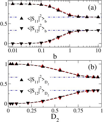
First we consider the case $M=1$, where the $S$-matrix is a $2\times 2$ matrix. In Fig. 2(a) we plot the ensemble average of the elements $|S_{11}|^{2}$ and $|S_{12}|^{2}$ as a function of the bandwidth parameter $b$, $\left\langle|S_{11}|^{2}\right\rangle_{b}$ and $\left\langle|S_{12}|^{2}\right\rangle_{b}$, for the periodic (black symbols) and the non-periodic (red symbols) PBRM model. We concentrate on these two matrix elements since the other two elements give no additional information: $\left\langle|S_{22}|^{2}\right\rangle_{b}=\left\langle|S_{11}|^{2}\right\rangle_{b}$ and $\left\langle|S_{21}|^{2}\right\rangle_{b}=\left\langle|S_{12}|^{2}\right\rangle_{b}$. Notice a strong $b$-dependence of the average $S$-matrix elements driving them from a localized-like regime [$\left\langle|S_{11}|^{2}\right\rangle\approx 1$ and $\left\langle|S_{12}|^{2}\right\rangle\approx 0$; i.e. the average conductance is close to zero] for $b\ll 1$, to a delocalized-like or ballistic-like regime [$\left\langle|S_{11}|^{2}\right\rangle\approx 2/3$ and $\left\langle|S_{12}|^{2}\right\rangle\approx 1/3$; i.e., RMT results are already recovered] for $b\geq 4$.

Moreover, we have found that $\left\langle|S_{11}|^{2}\right\rangle$ and $\left\langle|S_{12}|^{2}\right\rangle$, as a function of the bandwidth $b$, are well described by

$$\left\langle|S_{11}|^{2}\right\rangle_{b} = 1-\left\langle|S_{12}|^{2}\right\rangle_{b}\ ,$$ (13)

$$\left\langle|S_{12}|^{2}\right\rangle_{b} = \frac{1}{3}\left[\frac{1}{1+(\delta b)^{-2}}\right]\ ,$$ (14)

where $\delta$ is a fitting parameter. Eq. (13) is a consequence of the unitarity of the scattering matrix, $SS^{\dagger}=\mathbf{1}$, while the factor 1/3 in Eq. (14) comes from Eq. (7) with $M=1$. In Fig. 2(a) we plot Eqs. (13) and (14) (dashed lines) and compare them with the corresponding results from the PBRM model (symbols) in the periodic and non-periodic setups. In the same figure Eq. (7) is also plotted (dot-dashed lines).

On the other hand, it is well known that in systems at the disorder driven MIT both the energy spectra and the eigenstates exhibit multifractal characteristics. EM08 The PBRM model is characterized by the effective bandwidth $b$ that drives the system from strong ($b\to 0$) to weak ($b\to\infty$) multifractality. Multifractality can be quantified by the generalized dimensions $D_{q}$ which describe the fluctuations of the eigenfunctions. The multifractal dimensions $D_{q}$ of the $\sigma$-th eigenfunction $\Psi^{\sigma}$ (given as a linear combination of the basis states in a system with linear size $L$, $\Psi^{\sigma}=\sum_{l=1}^{L}C_{l}^{\sigma}\phi_{l}$) are defined through the so-called inverse participation numbers, ${\cal I}_{q}=\sum_{l=1}^{L}\left|C_{l}^{\sigma}\right|^{2q}$, by the scaling EM08 ; EM00a ; V03

$$({\cal I}_{q})^{\mbox{\tiny typ}}\propto L^{-(q-1)D_{q}}\ ,$$ (15)

where $({\cal I}_{q})^{\mbox{\tiny typ}}=\exp\left\langle\ln{\cal I}_{q}\right\rangle$ is the typical value of ${\cal I}_{q}$. However, among all dimensions, the correlation dimension $D_{2}$ plays a prominent role. HP83 As $b$ transits from zero to infinity, $D_{2}$ takes values from zero to one.

Using numerical diagonalization of matrices with sizes $L=128$, 256, 512, and 1024, we extracted $D_{2}$ by the use of Eq. (15). For each system size $L$, we used a number of disorder realizations in order to have at least $10^{5}$ data for its analysis. For each disorder realization we used $25\%$ of the states at the centre of the spectral band (where the density of states is almost constant) in order to avoid boundary effects. We found good agreement between the numerically obtained $D_{2}$ and the analytical estimation EM08 ; EM00a

$$D_{2}=\left\{\begin{array}[]{ll}2b\ ,&\quad b\ll 1\\ 1-(\pi b)^{-1}\ ,&\quad b\gg 1\end{array}\right.\ .$$

Moreover, in Ref. [MKC05, ] the following phenomenological analytical expression for $D_{2}$ as a function of $b$ was proposed:

$$D_{2}(b)=\frac{1}{1+(\gamma b)^{-1}}\ ,$$ (16)

where $\gamma$ is a fitting parameter. See also Ref. [MI06, ]. Eq. (16) describes well our numerical results for $D_{2}$ with $\gamma=2.94$ and $\gamma=2.88$ for the periodic and non-periodic versions of the PBRM model, respectively.

Figure 3: (Color online) (a) Black [red (gray)] curves: Probability distribution $\rho(\ln T)$ for the periodic [non-periodic] PBRM model at criticality for several values of $b<1$ ($b=0.01$, 0.02, 0.04, 0.1, 0.2, and 0.4 from left to right) in the case $M=1$. (b) Black [red (gray)] symbols: $\left\langle\ln T\right\rangle$ as a function of $b$ for the periodic [non-periodic] PBRM model. The blue (gray) dashed line is the best fit of the data to the logarithmic function $A+\ln b^{2}$ with $A\approx-1.44$. (c) $\rho(\ln T)$ for $b<1$ scaled to $T_{\mbox{\tiny typ}}=\exp\langle\ln T\rangle\sim b^{2}$. The blue (gray) dashed line proportional to $(T/T_{\mbox{\tiny typ}})^{1/2}$ is plotted to guide the eye.

Figure 4: (Color online) Black [red (gray)] curves: Conductance probability distribution $w(T)$ for the periodic [non-periodic] PBRM model at criticality for some large values of $b$ in the case $M=1$. Blue (gray) dashed lines are $w(T)_{\mbox{\tiny COE}}$; the RMT prediction for $w(T)$ given by Eq. (8).

Figure 5: (Color online) (a) Black [red (gray)] curves: Probability distribution $\rho(\ln T)$ for the periodic [non-periodic] PBRM model at criticality for several values of $b<1$ ($b=0.01$, 0.02, 0.04, 0.1, and 0.2 from left to right) in the case $M=2$. (b) Black [red (gray)] symbols: $\left\langle\ln T\right\rangle$ as a function of $b$ for the periodic [non-periodic] PBRM model. The blue (gray) dashed line is the best fit of the data to the logarithmic function $A+\ln b^{2}$ with $A\approx-0.057$. (c) $\rho(\ln T)$ for $b<1$ scaled to $T_{\mbox{\tiny typ}}=\exp\langle\ln T\rangle\sim b^{2}$. The blue (gray) dashed line proportional to $(T/T_{\mbox{\tiny typ}})^{2}$ is plotted to guide the eye.

Figure 6: (Color online) Black [red (gray)] curves: Conductance probability distribution $w(T)$ for the periodic [non-periodic] PBRM model at criticality for some large values of $b$ in the case $M=2$. Blue (gray) dashed lines are $w(T)_{\mbox{\tiny COE}}$; the RMT prediction for $w(T)$ given by Eq. (9).

Figure 7: (Color online) (a) Average conductance $\left\langle T\right\rangle$ as a function of $M$ for the non-periodic PBRM model at criticality for several values of $b$. $\left\langle T\right\rangle$ for the 3D Anderson model at criticality (3DAM) is also shown. (b) $\left\langle T\right\rangle/\left\langle T\right\rangle_{\mbox{\tiny COE}}$ as a function of $b\delta$ for the periodic PBRM model at criticality for $M\in[1,5]$. Insert: $\delta$ versus $M$. $\delta$ is obtained from the fitting of Eq. (22) to the $\left\langle T\right\rangle$ vs. $b$ data. Thick full lines correspond to $\left\langle T\right\rangle=0$. Blue (gray) dashed lines are (a) the RMT prediction for $\left\langle T\right\rangle$ given by Eq. (10); and (b) one.

Figure 8: (Color online) (a) Variance of $T$ as a function of $M$ for the non-periodic PBRM model at criticality for several values of $b$. $\mbox{var}(T)$ for the 3D Anderson model at criticality (3DAM) is also shown. (b) $\mbox{var}(T)/\mbox{var}(T)_{\mbox{\tiny COE}}$ as a function of $b\delta$ for the periodic PBRM model at criticality for $M\in[1,5]$. Insert: $\delta$ versus $M$. $\delta$ is obtained from the fitting of Eq. (22) to the $\mbox{var}(T)$ vs. $b$ data. Thick full lines correspond to $\mbox{var}(T)=0$. Blue (gray) dashed lines are (a) the RMT prediction for $\mbox{var}(T)$ given by Eq. (11); and (b) one.

Figure 9: (Color online) (a) Shot noise power $P$ as a function of $M$ for the non-periodic PBRM model at criticality for several values of $b$. $P$ for the 3D Anderson model at criticality (3DAM) is also shown. (b) $P/P_{\mbox{\tiny COE}}$ as a function of $b\delta$ for the periodic PBRM model at criticality for $M\in[1,5]$. Insert: $\delta$ versus $M$. $\delta$ is obtained from the fitting of Eq. (22) to the $P$ vs. $b$ data. Thick full lines correspond to $P=0$. Blue (gray) dashed lines are (a) the RMT prediction for $P$ given by Eq. (12); and (b) one.

Then, by substituting Eq. (16) into Eqs. (13) and (14) we obtain the following expressions for the averages of $|S_{11}|^{2}$ and $|S_{12}|^{2}$ as a function of $D_{2}$:

$$\left\langle|S_{11}|^{2}\right\rangle_{D_{2}} = 1-\left\langle|S_{12}|^{2}\right\rangle_{D_{2}}\ ,$$ (17)

$$\left\langle|S_{12}|^{2}\right\rangle_{D_{2}} = \frac{1}{3}\frac{1}{1+(\gamma/\delta)^{2}\left(D_{2}^{-1}-1\right)^{2}}\ .$$ (18)

In Fig. 2(b) we compare Eqs. (17) and (18) (dashed lines) with the ensemble-average numerical results at different values of $D_{2}$. The agreement is excellent. In addition, it is interesting to note that

$$\left\langle|S_{12}|^{2}\right\rangle_{D_{2}}\propto\left\{\begin{array}[]{ll}D_{2}^{2}\ ,&\quad D_{2}\to 0\\ 1-(\gamma/\delta)^{2}\left(D_{2}^{-1}-1\right)^{2}\ ,&\quad D_{2}\to 1\end{array}\right.\ ,$$

which might be relevant for systems at the MIT where $D_{2}$ can be tuned.

Finally we want to remark that concerning $\left\langle|S_{aa^{\prime}}|^{2}\right\rangle$ for the PBRM model, the RMT limit, expected for $b\to\infty$, is already recovered for $b\geq 4$. See Fig. 2(a).

$L$	$b=0.1$	$b=1$	$b=10$
50	$-5.887\pm 0.002$	$-2.249\pm 0.002$	$-2.001\pm 0.002$
100	$-5.886\pm 0.002$	$-2.247\pm 0.002$	$-1.999\pm 0.002$
200	$-5.875\pm 0.002$	$-2.245\pm 0.002$	$-1.999\pm 0.002$
400	$-5.875\pm 0.002$	$-2.244\pm 0.002$	$-2.002\pm 0.002$
800	$-5.869\pm 0.002$	$-2.228\pm 0.002$	$-1.989\pm 0.002$

Table 1: $\left\langle\ln T\right\rangle$ for the periodic PBRM model at criticality for some values of $b$ and $L$ in the case $M=1$.

II.2 Conductance probability distribution

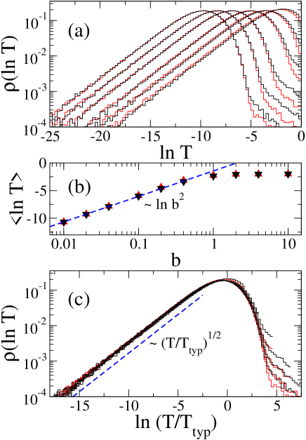
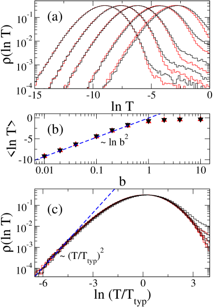
Now we turn to the conductance statistics. For $b\ll 1$ the conductance distribution $w(T)$ is highly concentrated close to $T=0$. So it is more convenient to analyse the distribution of the transmission logarithm, $\rho(\ln T)$, instead. Then, in Fig. 3(a) we show $\rho(\ln T)$ for several values of $b<1$ in the case $M=1$, for the periodic and non-periodic versions of the PBRM model. Notice that the distribution functions $\rho(\ln T)$ do not change their shape by increasing $b$, mainly for $b\ll 1$, thus being scale invariant. In fact, $\left\langle\ln T\right\rangle$ for $b<1$ clearly displays a linear behavior when plotted as a function of $\ln b$ as shown in Fig. 3(b). Then, all distributions functions $\rho(\ln T)$ fall one on top of the other when shifting them along the $x$-axis by the typical value of $T$,

$$T_{\mbox{\tiny typ}}=\exp\langle\ln T\rangle\ ,$$ (19)

as shown in Fig. 3(c).

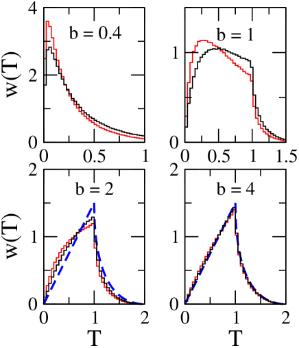
Note that for $T<T_{\mbox{\tiny typ}}$, $\rho(\ln T)$ is proportional to $(T/T_{\mbox{\tiny typ}})^{1/2}$, see Figs. 3(a) and 3(c). Moreover, we found that such behavior extends from small to large values of $b$, $b\gg 1$. Also, notice that the behavior $\rho(\ln T)\propto T^{1/2}$ for small $T$ coincides with the RMT prediction $w(T)_{\mbox{\tiny COE}}\propto T^{-1/2}$, see Eq. (8), since the change of variable $T\to\ln T$ leads to $\rho(\ln T)=Tw_{\mbox{\tiny COE}}(T)$.

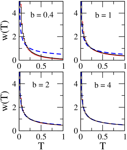
In Fig. 4 we show $w(T)$ for large $b$ ($b\geq 0.4$). In the limit $b\to\infty$, $w(T)$ is expected to approach the RMT prediction of Eq. (8). However, once $b\geq 4$, $w(T)$ is already well described by $w(T)_{\mbox{\tiny COE}}$.

We want to stress that our results do not depend on the system size $L$, as can be seen in Table 1 where we report $\left\langle\ln T\right\rangle$ for the periodic PBRM model at criticality for some values of $b$ and $L$ in the case $M=1$. In fact, $\left\langle\ln T\right\rangle$ does not depend on $L$ out of criticality ($\alpha>1$ and $\alpha<1$) either. This makes an important difference with respect to the setup where the leads are attached to opposite sides of the sample where $\left\langle\ln T\right\rangle$ increases (decreases) as a function of $L$ for $\alpha<1$ ($\alpha>1$ and $\alpha=1$).

Now, in Figs. 5 and 6 we explore $w(T)$ in the case $M=2$. As well as in the case $M=1$, studied above, here: (i) for small $b$, $\rho(\ln T)$ is scale invariant with $T_{\mbox{\tiny typ}}$ as scaling factor, see Fig. 5; (ii) for $b\geq 4$, $w(T)$ is well described by Eq. (9), the corresponding RMT prediction, see Fig. 6. However, although $\rho(\ln T)$ for small $b$ and $w(T)$ for large $b$ are practically the same for the periodic and non-periodic versions of the PBRM model, they show differences for intermediate values, $0.1<b<4$, as can be seen in Fig. 5(a) and the upper panels of Fig. 6.

We point out that for small $T$, $T\ll T_{\mbox{\tiny typ}}$, $\rho(\ln T)$ is proportional to $(T/T_{\mbox{\tiny typ}})^{2}$, as shown in Fig. 5(c). This behavior is universal for the PBRM model with $M=2$; i.e. it is $b$-independent and valid for the periodic and non-periodic versions of the model. Again, as for the $M=1$ case, here for $M=2$, the dependence $\rho(\ln T)\propto T^{2}$ in the limit $b\to\infty$ is consistent with the RMT prediction $w(T)_{\mbox{\tiny COE}}\propto T$ for $T<1$; see Eq. (9).

From the results above and since MK04

$$w(T)_{\mbox{\tiny COE}}\propto T^{M^{2}/2-1}\ ,$$ (20)

in the region $0<T<1$, we conclude that for the PBRM model

$$\rho(\ln T)\propto T^{M^{2}/2}\ ,$$ (21)

for $T\ll T_{\mbox{\tiny typ}}$. We argue that the behavior dictated by Eq. (21) can be interpreted in the following way: Since small values of conductance $T\ll 1$ mean very strong reflection, the scattering process is almost direct, i.e. an incident electron is scattered out the system mainly by the interaction with the sites at which the leads are attached. Then the electron does not explore the complete sample, not even part of it, and as a consequence it does not realize that the sample is at criticality. That is, for $T\ll 1$, the incident electron does not distinguish between a critical system and a random system represented by a full random matrix if the number of attached leads $2M$ is not much larger than $b$; i.e., when the leads are attached to sites interconnected by Hamiltonian matrix elements located within the bandwidth of the matrix where all elements have almost the same variance: $\left\langle|H_{ij}|^{2}\right\rangle\approx 1/2$. So, we can use Eq. (20) and as a consequence Eq. (21) too. In fact, we have verified that Eq. (21) is valid up to $M=2$ for $b\leq 1$, while for $b=10$ it describes perfectly the left tail of $\rho(\ln T)$ for all the values of $M$ used in this work (up to $M=5$). Our result, given by Eq. (21), is the generalization of the result shown in Ref. [MG09a, ], where the behavior $\rho(\ln T)\propto T^{1/2}$ was reported for the PBRM model in the localized ($\alpha>1$) and delocalized regimes ($\alpha<1$) for $M=1$.

II.3 Mean and variance of the conductance and the shot noise power

Figure 10: Probability distribution $\rho(\ln T)$ for the 3D Anderson model at criticality in the cases $M=1$ and $M=2$. Dashed lines with slopes $T^{1/2}$ and $T^{2}$ are plotted to guide the eye.

Figure 11: (Color online) Conductance probability distribution $w(T)$ for the 3D Anderson model at criticality in the cases (a) $M=1$ and (b) $M=2$. The red (gray) dashed line corresponds to $w(T)$ for the non-periodic PBRM model with $b=0.2$.

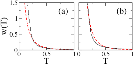
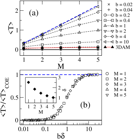
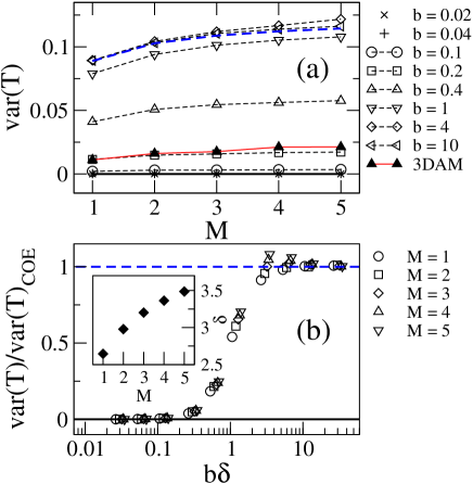
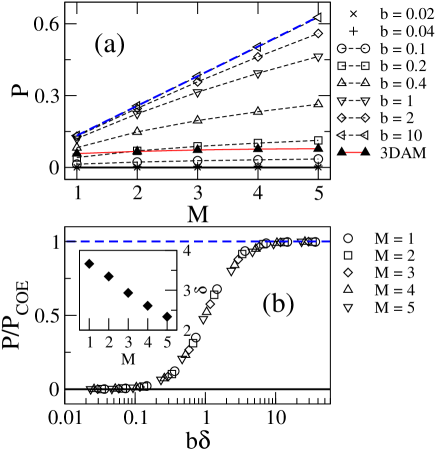
We now increase further the number of attached leads. In Figs. 7(a), 8(a), and 9(a) we plot the average conductance $\left\langle T\right\rangle$, the variance of the conductance $\mbox{var}(T)$, and the shot noise power $P$ for the non-periodic version of the PBRM model for several values of $b$ with $M\in[1,5]$. It is clear from these three plots that changing $b$ from small ($b\ll 1$) to large ($b>1$) values produces a transition from localized- to delocalized-like behavior in the scattering properties of the PBRM model. That is, (i) for $b<0.1$, $\left\langle T\right\rangle\approx 0$, $\mbox{var}(T)\approx 0$, and $P\approx 0$; and (ii) for $b\geq 10$, $\left\langle T\right\rangle$, $\mbox{var}(T)$, and $P$ are well described by the corresponding RMT predictions given by Eqs. (10), (11), and (12), respectively. Similar plots are obtained (not shown here) for the periodic PBRM model.

Moreover, we have observed that $\left\langle T\right\rangle$, $\mbox{var}(T)$, and $P$ behave (for all $M$) as $\left\langle|S_{12}|^{2}\right\rangle_{b}$ does. See Eq. (14). Thus, we can write

$$X(b)=X_{\mbox{\tiny COE}}\left[\frac{1}{1+(\delta b)^{-2}}\right]\ ,$$ (22)

where $X$ represents $\left\langle T\right\rangle$, $\mbox{var}(T)$, or $P$ and $\delta$ is a fitting parameter. Then, in Figs. 7(b), 8(b), and 9(b) we plot $\left\langle T\right\rangle$, $\mbox{var}(T)$, and $P$ normalized to their respective COE average values, now for the periodic PBRM model as a function of $b\delta$ for $M\in[1,5]$. Also, similar plots are obtained (not shown here) for the non-periodic PBRM model.

III 3D Anderson model

Since the most prominent realization of systems that undergo a MIT is the 3D Anderson model, it is of relevance to analyse its scattering and transport properties taking as a reference the results shown in the previous section for the PBRM model.

We attach the $2M$ leads to $2M$ sites at one of the edges of the cubic lattice described by the 3D Anderson model. In this way we make a line contact as we did in the case of the PBRM model. So, we can compare the scattering properties of both models. We use Gaussian distributed on-site potentials and system sizes from $L=6$ to 10 (we have verified that our results do not change by increasing $L$ further) with $10^{6}$ to $10^{4}$ disorder realizations.

We start our analysis by looking at the average scattering matrix elements for $M=1$. For the 3D Anderson model at criticality we found $\left\langle|S_{11}|^{2}\right\rangle\approx 0.926$ and $\left\langle|S_{12}|^{2}\right\rangle\approx 0.074$, see Table 2, which are close to those of the non-periodic PBRM model with $b=0.24$.

In Fig. 10 we show conductance probability distributions $\rho(\ln T)$ for the 3D Anderson model at criticality in the cases $M=1$ and $M=2$. We found $\left\langle\ln T\right\rangle\approx-3.47$ and $-3.06$ for $M=1$ and $M=2$, respectively. See Table 3. These values of $\left\langle\ln T\right\rangle$ for the 3D Anderson model are close to those of the PBRM model with $b=0.36$ and $b=0.22$, respectively. Notice also that, as well as for the PBRM model, for the 3D Anderson model $\rho(\ln T)$ in the region of $T\ll T_{\mbox{\tiny typ}}$ is proportional to $(T/T_{\mbox{\tiny typ}})^{1/2}$ and $(T/T_{\mbox{\tiny typ}})^{2}$ for $M=1$ and $M=2$, respectively (dashed lines in Fig. 10).

Additionally, in Fig. 11 we plot $w(T)$ for the 3D Anderson model in the cases $M=1$ and $M=2$. In the same figure we have also plotted (dashed lines) the conductance distributions from the PBRM model with $b=0.2$. We can see that the conductance distributions of both models are similar at this bandwidth value.

$L$	$\left\langle|S_{11}|^{2}\right\rangle$	$\left\langle|S_{12}|^{2}\right\rangle$
6	$0.9256\pm 0.0001$	$0.0743\pm 0.0001$
8	$0.9254\pm 0.0003$	$0.0745\pm 0.0003$
10	$0.926\pm 0.001$	$0.073\pm 0.001$

Table 2: Average $S$-matrix elements $\left\langle|S_{11}|^{2}\right\rangle$ and $\left\langle|S_{12}|^{2}\right\rangle$ for the 3D Anderson model at criticality for some values of $L$ in the case $M=1$.

$L$	$\left\langle\ln T\right\rangle(M=1)$	$\left\langle\ln T\right\rangle(M=2)$
6	$-3.471\pm 0.001$	$-3.060\pm 0.001$
8	$-3.483\pm 0.005$	$-3.058\pm 0.003$
10	$-3.450\pm 0.016$	$-3.078\pm 0.012$

Table 3: $\left\langle\ln T\right\rangle$ for the 3D Anderson model at criticality for some values of $L$ in the cases $M=1$ and $M=2$.

We also compute $\left\langle T\right\rangle$, $\mbox{var}(T)$, and $P$ for the 3D Anderson model and plot them in Figs. 7(a), 8(a), and 9(a), respectively (red curves labeled as 3DAM). We observe that for the 3D Anderson model $\left\langle T\right\rangle$, $\mbox{var}(T)$, and $P$ behave as the corresponding quantities for the PBRM model with $b$ close to 0.2.

We want to stress that our results for the 3D Anderson model at criticality do not seem to depend on the on-site potential distribution. Here we used Gaussian distributed potentials. However, we observe practically the same results by the use of box distributed on-site potentials (not shown here).

IV Conclusions

We study the scattering and transport properties of the Power-law Banded Random Matrix (PBRM) model and of the three-dimensional (3D) Anderson model, both at criticality.

We observed a smooth crossover from localized- to delocalized-like (ballistic-like) behavior in the scattering properties of the PBRM model by varying $b$ from small ($b\ll 1$) to large ($b>1$) values. For this crossover region we proposed heuristic analytical expressions for $\langle|S_{aa^{\prime}}|^{2}\rangle_{b}$ and $\langle|S_{aa^{\prime}}|^{2}\rangle_{D_{2}}$. For small $b$, we have shown that $\rho(\ln T)$ is scale invariant with the typical value of $T$, $T_{\mbox{\tiny typ}}$, as scaling factor. We realized that RMT results, expected in the limit $b\to\infty$, are already recovered for relatively small values of the bandwidth: $b\geq 10$. However, this fact is closely related to the small number of attached leads we used in this work: the larger the number of leads the larger the value of $b$ needed to approach RMT behavior.

Our conclusions are valid for leads attached to the bulk of the system as well as for leads attached at the boundary. In this work we assumed that time-reversal symmetry ($\beta=1$) is present in our disordered systems. Moreover, the case of broken time-reversal symmetry ($\beta=2$) has been preliminarily studied in Ref. [AMV09, ] where similar conclusions to this work were made.

We have also shown that the scattering properties of the 3D Anderson model are similar to those for the PBRM model with $b\in[0.2,0.4]$. This result is in agreement with previous studies EM00b were it was shown that several critical quantities related to the spectrum and eigenstates of the PBRM model with $b=0.3$ are practically the same as for the 3D Anderson model. This makes the PBRM model an excellent candidate to explore the properties of the 3D Anderson model at criticality at a low computational cost.

We want to stress that for both models at criticality, the PBRM model and the 3D Anderson model, we found the universal behavior $\rho(\ln T)\propto T^{M^{2}/2}$ for $T\ll 1$, that we tested here for $M=1$ and $M=2$. Moreover by the use of the PBRM model with $\beta=2$ (not shown here) we have already verified that the more general expression $\rho(\ln T)\propto T^{\beta M^{2}/2}$, derived from MK04 $w(T)\propto T^{\beta M^{2}/2-1}$ with $0<T<1$, holds.

We emphasize that, even though we used a scattering setup where the leads are attached perfectly to sites at one side of the sample, our conclusions are not restricted to this topology.unpublished

Finally, we recall that we concentrate here on the case of a small number of single-channel attached leads (up to ten). The study of the scattering and transport properties of the PBRM and the 3D Anderson models in the regime of $M\gg 1$ will be the subject of a forthcoming contribution.