Partially integrable dynamics of ensembles of nonidentical oscillators

Abstract

We consider ensembles of sine-coupled phase oscillators consisting of subpopulations of identical units, with a general heterogeneous coupling between subpopulations. Using the Watanabe-Strogatz ansatz we reduce the dynamics of the ensemble to a relatively small number of dynamical variables plus microscopic constants of motion. This reduction is independent of the sizes of subpopulations and remains valid in the thermodynamic limits, where these sizes or/and the number of subpopulations are infinite. We demonstrate that the approach to the dynamics of such systems, recently proposed by Ott and Antonsen, corresponds to a particular choice of microscopic constants of motion. The theory is applied to the standard Kuramoto model and to the description of two interacting subpopulations, exhibiting a chimera state. Furthermore, we analyze the dynamics of the extension of the Kuramoto model for the case of nonlinear coupling and demonstrate the multistability of synchronous states.

1 Introduction

A model of all-to-all, or globally coupled limit cycle oscillators explains many natural phenomena in various branches of science. The applications range from the description of the collective dynamics of Josephson junctions [1], lasers [2], and electrochemical oscillators [3] to that of pedestrians on footbridges [4, 5], applauding persons in a large audience [6], cells, exhibiting glycolitic oscillations [7, 8, 9], neuronal populations [10], etc. Externally forced or feedback controlled globally coupled ensemble or several interacting ensembles serve as models of circadian rhythms, normal and pathological brain activity, interaction of different brain regions, and many other problems [11, 12, 13, 14, 15, 16, 17]. Many aspects of the ensemble dynamics, especially those related to inhomogeneity [18, 19, 20] or nonlinearity of coupling [21, 22], temporal dynamics of the collective mode [23, 24], different frequency distributions [25, 26], and clustering [27, 28, 29] remain in the focus of the current research activity.

Ensembles of weakly interacting units are successfully treated within the framework of phase approximation [30, 31, 32, 33, 34]. Most popular is the Kuramoto model of sine-coupled phase oscillators. This model explains self-synchronization and appearance of a collective mode (mean field) in an ensemble of generally non-identical elements; the transition to synchrony occurs at a certain critical value of the coupling constant that is roughly proportional to the width of the distribution of natural frequencies [30, 31]. With the further increase of coupling, more and more oscillators join synchronous cluster, so that the amplitude of the mean field grows as a square root of supercriticality. It is instructive to interprete this transition as follows: the non-zero mean field forces individual units and entrains at least a part of them; these entrained units become coherent, thus yielding a non-zero mean field. A quantitative consideration, based on this argument and first performed by Kuramoto [30, 31], provides the amplitude and frequency of the stationary solution. References to many further aspects of the Kuramoto model can be found in [35, 36, 37].

An extension of the Kuramoto model for the case of nonlinear coupling has been suggested in our recent publications [21, 22], where the most simple case of identical units has been treated. Nonlinearity in this context means that the effect of the collective mode on an individual unit depends on the amplitude of this forcing, so that, e.g., the interaction of the field and a unit can be attractive for weak forcing and repulsive for strong one. This can lead to nontrivial effects like a destruction of a completely synchronous state and appearance of partial synchrony in an ensemble of identical units. Moreover, in this state the frequencies of the collective mode and of oscillators can be different and incommensurate. The analysis of the nonlinear model for the case of an ensemble with a frequency distribution is still lacking and will be performed below. This analysis is based on the extension of the Watanabe–Strogatz (WS) theory [38, 39] to the case of nonidentical oscillators, suggested in our brief communication [40].

For a population of identical oscillators, a full dynamical description of the Kuramoto model can be obtained with the help of the WS ansatz which reduces the dynamics to that of three macroscopic variables plus constants of motion. This works even for a nonlinear coupling [22]. The main idea of this paper is in extending the WS ansatz on an ensemble of nonidentical oscillators, treating it as a system of coupled subpopulations, each consisting of identical oscillators. Each subpopulation can be then described by three WS variables, whereas the full system is described by a system of coupled WS equations. A description of an ensemble with a continuous frequency distribution is then obtained by performing a thermodynamic limit. The extended WS approach is applied to a population of oscillators with a Lorentzian frequency distribution (the standard Kuramoto model), and to a population of identical oscillators with inhomogeneous coupling [18]. In particular, within this framework we establish a relation between the WS approach and the recent Ott-Antonsen (OA) ansatz [23, 24], which yields, under certain assumptions, a dynamical equation for the evolution of the mean field. In this paper we discuss in detail how the WS theory can be applied to populations of non-identical units and apply this approach to describe the dynamics of oscillator ensembles with global nonlinear coupling, for the case of Lorentzian distribution of frequencies.

The paper is organized as follows. We discuss the main model in Section 2. Extension of the WS theory to the case of nonidentical oscillators is presented in Section 3. In Section 4 we discuss a relation between the WS theory and the OA ansatz (cf. a recent paper by Marvel, Mirollo, and Strogatz [41] for a related discussion). This theory is applied to describe the dynamics of linearly (Section 5) and nonlinearly (Section 6) coupled ensembles; here we also support the theory by numerics. In particular, we demonstrate the differences of the dynamics of the full equation system and that confined to the OA reduced manifold. We summarize and discuss our results in Section 7.

2 Hierarchically organized population of oscillators

In this Section we introduce a model of hierarchically organized populations of oscillators and describe it in terms of microscopic equations of motion. The main idea is to treat an ensemble of nonidentical oscillators as a collection of subpopulations of identical oscillators.

We start by introducing an ensemble of nonidentical phase oscillators, characterized by phase variables $\phi_{k}$ and generally time-dependent frequencies $\omega_{k}(t)$, where $k=1,\ldots,N$ is the oscillator index and $N$ is the ensemble size. Each oscillator generally interacts with all other units and is subject to external fields. The effect of these interactions can be represented as some effective forcing and therefore each unit is described as a driven oscillator

$$\frac{d\phi_{k}}{dt}=\omega_{k}(t)+A_{k}(t)\sin(\xi_{k}(t)-\phi_{k})\;,\quad k=1,\ldots,N\;,$$ (1)

where variables $A_{k}$ and $\xi_{k}$ characterize the amplitude and phase of the force. It is convenient to introduce a complex force $H_{k}=A_{k}e^{i\xi_{k}}$ and re-write Eq. (1) as

$$\frac{d\phi_{k}}{dt}=\omega_{k}+\mbox{Im}\left(H_{k}e^{-i\phi_{k}}\right)\;.$$ (2)

In many particular cases considered below the force $H$ is calculated in some mean-field manner from the state of the whole population or some subpopulation(s). However, for a while we prefer to consider $H$, as well as $\omega$, as arbitrary functions of time; for brevity we skip this dependence in the notations. Note that generally $H$ can include random component(s) which describe a forcing by common noise. We emphasize that Eqs. (2) do not represent the most general model of coupled phase oscillators, because the high order harmonic components of the phase $\sim e^{-in\phi_{k}}$, with $n>1$, do not appear on the right hand side of Eqs. (2).

Figure 1: Hierarchically organized ensemble (left panel) can be considered as a collection of subpopulations labeled by index $a=1,\ldots,M$, with a generally bidirectional asymmetrical coupling between subpopulations. Generally, the subpopulations are exposed to external field(s). Each subpopulation (right panel) of the oscillator ensemble consists of identical oscillators driven by a common force. This force results from the action of all other subpopulations and external fields and from the coupling within the subpopulation, which is usually taken to be of a mean field type. This means that outputs of all oscillators create the mean field that acts back on these oscillators. The crucial point is that the forcing is formed either via linear or nonlinear transformation of acting mean fields.

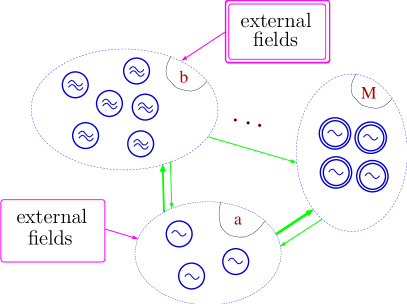
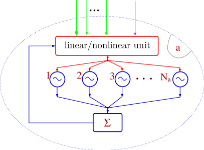
In general, all oscillators described by (2) have different dynamics, and such a system cannot be further reduced. Such a simplification is possible for an ensemble of identical oscillators, where the WS theory holds which states that dynamics of a population of identical oscillators of type (2) subject to a common forcing is effectively three-dimensional (this is discussed in details in the next Section). In order to make use of the WS ansatz to an ensemble of nonidentical oscillators, we assume that this ensemble consists of groups (subpopulations) of identical units (Fig. 1, cf. [42]). Accordingly, we re-label the oscillators grouping them into $M$ subpopulations, denoted by index $a$. Each population contains $N_{a}$ identical units with frequency $\omega_{a}$ which are driven by a common force $H_{a}$. The equations now read:

$$\frac{d\phi_{k}^{(a)}}{dt}=\omega_{a}+\mbox{Im}\left(H_{a}e^{-i\phi_{k}^{(a)}}\right)\;,$$ (3)

where $k=1,\ldots,N_{a}$ and $a=1,\ldots,M$, with an obvious relation $\sum_{a=1}^{M}N_{a}=N$. Note that two subpopulations can have the same frequencies $\omega_{a}=\omega_{b}$ but differ by the force $H_{a}\neq H_{b}$, or they can have different frequencies but the same force, or they can differ both by their frequencies and the forces.

Certainly, such grouping of oscillators into subpopulations is not always possible (if we exclude a trivial case when each subpopulation contains one unit and $M=N$). However, in many particular cases $M\ll N$ and the description of the dynamics simplifies essentially: as we will see in the next Section, each group is described by three WS variables and instead of $N$ equations (3) we have to deal with $M$ coupled systems of three WS equations each. Note that WS ansatz is also valid for infinitely large populations of identical oscillators. Thus, if some or all of subpopulation sizes $N_{a}\to\infty$, we still obtain a $3M$-dimensional description of the collective dynamics. As discussed in the next Section, the idea to consider an ensemble as a collection of subpopulations is also fruitful for treating a thermodynamic limit $N\to\infty$ with a continuous distribution of oscillator frequencies.

3 Oscillator populations in external fields

In this Section we discuss the dynamics of large populations of oscillators subject to an arbitrary external force. First, we briefly present the WS theory which treats ensembles of identical oscillators. We re-write the WS equations in new notations, what makes them more convenient for the consequent analysis. Next, we extend the WS theory to the case of a finite number of interacting groups. Finally, performing a thermodynamic limit, we obtain a description of an ensemble with a continuous frequency distribution.

3.1 Identical oscillators

First we discuss in details dynamics of a population of identical oscillators subject to an arbitrary forcing, which is, however, common for all oscillators.

3.1.1 WS equations

The main result of the seminal papers by Watanabe and Strogatz [38, 39] is that a population of $N>3$ sine-coupled phase oscillators with any time-dependent common frequency $\omega(t)$, driven by an arbitrary but common force $H(t)$,

$$\frac{d\phi_{k}}{dt}=\omega(t)+\mbox{Im}\left(H(t)e^{-i\phi_{k}}\right)\;,\quad k=1,\ldots,N\;,$$ (4)

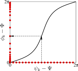
can be completely described by three global variables $\rho(t)$, $\Phi(t)$, and $\Psi(t)$ plus constants of motion $\psi_{k}$ that are determined by initial conditions. The original phases can be recovered by means of the time-dependent transformation

$$e^{i\phi_{k}}=e^{i\Phi}\frac{\rho+e^{i(\psi_{k}-\Psi)}}{\rho e^{i(\psi_{k}-\Psi)}+1}\;,$$ (5)

or, equivalently,

$$\tan\left(\frac{\phi_{k}-\Phi}{2}\right)=\frac{1-\rho}{1+\rho}\tan\left(\frac{\psi_{k}-\Psi}{2}\right)\;,$$ (6)

see Fig. 2 for illustration.

Here $\psi_{k}$ are the constants of motion. Notice that only $N-3$ of them are independent; see the discussion below. The time-dependent functions $\rho(t)$, $\Phi(t)$, and $\Psi(t)$ are the global amplitude and phase variables, respectively. In the following we denote them as WS variables, their meaning is discussed later. For the transformation (5) to be consistent with equations of motion (4), these variables have to obey the WS equations

$$\frac{d\rho}{dt} =\frac{1-\rho^{2}}{2}\mbox{Re}(He^{-i\Phi})\;,$$ (7)

$$\frac{d\Phi}{dt} =\omega+\frac{1+\rho^{2}}{2\rho}\mbox{Im}(He^{-i\Phi})\;,$$ (8)

$$\frac{d\Psi}{dt} =\frac{1-\rho^{2}}{2\rho}\mbox{Im}(He^{-i\Phi})\;.$$ (9)

We emphasize that we use the global variables slightly different from those originally used by WS [39] and write the equations in a different form. The relation to the original form can be found in Appendix A; there we also demonstrate the equivalence of the transformations (5) and (6).

Figure 2: Illustration of the transformation $\psi_{k}\to\phi_{k}$, see Eqs. (5,6), here for $\rho=0.5$ (cf. Fig. 3 in [39]).

For a further analysis it is convenient to introduce a combination of two WS variables $z=\rho e^{i\Phi}$. We call this complex variable the bunch amplitude. Introducing also the phase shift $\alpha=\Phi-\Psi$, we write the WS equations (7-9) in an equivalent form:

$$\frac{dz}{dt} =i\omega z+\frac{1}{2}H-\frac{z^{2}}{2}H^{*}\;,$$ (10)

$$\frac{d\alpha}{dt} =\omega+\text{Im}(z^{*}H)\;.$$ (11)

3.1.2 Constants of motion

Transformation (5) from original variables $\phi_{k}$ to WS variables $\rho$, $\Phi$, $\Psi$ (or $z$ and $\alpha$) and $\psi_{k}$ yields an overdetermined system. Hence, we have to impose $3$ constraints on the constants $\psi_{k}$; this is discussed in detail in [39]. It is convenient to choose two constraints as follows:

$$\sum_{k=1}^{N}e^{i\psi_{k}}=0\;.$$ (12)

The third constraint on $\psi_{k}$ is somehow arbitrary, it only fixes the common shift of $\psi_{k}$ with respect to $\Psi$. It can be taken, e.g., as $\sum_{k}\psi_{k}=0$ (this implies that constants are defined in the $[-\pi,\pi]$ interval) [39]. Another convenient choice is $\sum\cos(2\psi_{k})=0$. The imposed constraints allow one to determine unambiguously the new variables $\rho(0)$, $\Psi(0)$, $\Phi(0)$ and constants $\psi_{k}$ from the initial conditions $\phi_{k}(0)$ and vice versa, this is discussed in details in Ref. [39].

3.1.3 Meaning of the WS variables

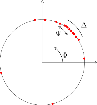
In order to discuss the physical meaning of the WS variables we compare them with the complex mean field, or the Kuramoto order parameter

$$Z=N^{-1}\sum_{k=1}^{N}e^{i\phi_{k}}=re^{i\Theta},$$ (13)

where $r$ and $\Theta$ are the amplitude and phase of the mean field, respectively. [The comparison here is qualitative; a quantitative relation is given in Section 4.]

The WS amplitude variable $\rho$ is roughly proportional to the mean field amplitude $r$. Indeed, if $\rho=0$, then from Eq. (5) with account of Eq. (12), we obtain $r=0$. Similarly, Eq. (5) shows that for $\rho=1$ all $\phi_{k}$ are equal, what yields $r=1$. For intermediate values $0<\rho<1$ the relation between $\rho$ and $r$ generally depends also on $\Psi$ and $\psi_{k}$.

The WS phase variable $\Phi$ characterizes the position of the maximum in the distribution of phases and is close to the phase of the mean field $\Theta$. They coincide for $\rho=r=1$; for $0<\rho<1$, $\Phi$ is shifted with respect to $\Theta$ by a factor, dependent on $\rho$, $\Psi$.

Figure 3: Illustration of the meaning of the WS variables. The global amplitude $\rho$ is related to the width $\Delta$ of the distribution of phases; $\rho=0$ if this distribution is uniform and $\rho=1$ if it collapses to a $\delta$-distribution. Thus, $\rho$ is roughly proportional to the mean field amplitude $r$. Angle variable $\Phi$ describes the position of the hump in the distribution; therefore it roughly corresponds to the phase $\Theta$ of the mean field. Angle variable $\Psi$ characterizes the motion of individual oscillators with respect to the hump.

The second WS phase variable $\Psi$ determines the shift of individual oscillators with respect to $\Phi$. From Eqs. (8,9) we obtain a useful relation:

$$\dot{\Psi}=\frac{1-\rho^{2}}{1+\rho^{2}}(\dot{\Phi}-\omega)\;.$$ (14)

As can be seen from Fig. 2 and Eq. (6), $\phi_{k}$ decreases by $2\pi$ if $\Psi$ grows by $2\pi$. Hence, the oscillator frequency is

$$\omega_{osc}=\langle\dot{\phi}_{k}\rangle=\langle\dot{\Phi}\rangle-\langle\dot{\Psi}\rangle\;.$$ (15)

3.1.4 Dynamics of WS variables

Here we discuss possible solutions of Eqs. (7-9) for given $\omega(t)$, $H(t)$. First, we note that these equations represent a skew system: the variable $\Psi$ does not enter Eqs. (7,8). Hence, one has to solve the two-dimensional system (7,8) and then obtain $\Psi(t)$ via Eq. (14). Next, the system (7-9) obviously admits a fully synchronous solution $\rho=1$, describing a synchronized cluster of identical oscillators: all in the same state. As it follows from Eq. (9), in this case $\Psi$ is an arbitrary constant and the global dynamics is described solely by an equation for $\Phi$. However, we cannot analyze stability of this solution for general functions $\omega(t)$, $H(t)$. We mention here a seemingly trivial state when $H_{0}=0$. Then $\rho$ is arbitrary, $\dot{\Phi}=\omega$, and $\Psi=const$. This solution appears in the nonlinear model treated below in Section 6.

It is instructive to find solutions of Eqs. (7-9) for an important particular case $\omega=\mbox{const}$ and $H(t)=H_{0}e^{i\nu t}$. For this case of a harmonic forcing, Eqs. (7-9) take the form:

$$\frac{d\rho}{dt} =\frac{1-\rho^{2}}{2}H_{0}\cos(\nu t-\Phi)\;,$$ (16)

$$\frac{d\Phi}{dt} =\omega+\frac{1+\rho^{2}}{2\rho}H_{0}\sin(\nu t-\Phi)\;,$$ (17)

$$\frac{d\Psi}{dt} =\frac{1-\rho^{2}}{2\rho}H_{0}\sin(\nu t-\Phi)\;.$$ (18)

Introducing the phase differences $\Delta=\displaystyle\frac{\pi}{2}+\Phi-\nu t$ and $\alpha=\Phi-\Psi$ we rewrite this system as an autonomous one

$$\frac{d\rho}{dt} =\frac{1-\rho^{2}}{2}H_{0}\sin\Delta\;,$$ (19)

$$\frac{d\Delta}{dt} =\omega-\nu+\frac{1+\rho^{2}}{2\rho}H_{0}\cos\Delta\;,$$ (20)

$$\frac{d\alpha}{dt} =\omega-\nu-H_{0}\rho\cos\Delta\;.$$ (21)

Remarkably, the system (19,20) is reversible, as it remains invariant under a transformation $\Delta\to-\Delta$, $t\to-t$. The system possesses two types of solutions, in dependence on the detuning $|\omega-\nu|$. For $|\omega-\nu|\leq H_{0}$ system (19,20) has one attractive and one repelling steady state solution: these fixed points are located symmetrically with respect to the involution $\Delta\to-\Delta$ and have coordinates $\rho=1$ and $\Delta=\pm\arccos\frac{|\omega-\nu|}{H_{0}}$, respectively. For the case $|\omega-\nu|>H_{0}$ the system has no attractors, and the exact solution, described in Appendix B, is represented by a family of closed orbits around a marginally stable equilibrium with coordinates $\Delta_{0}=0$ and $\rho_{0}$ (see Eq. (97)). For this equilibrium solution, $\Psi$ rotates with a constant frequency, given by Eq. (98). Except for this special case, the variables $\rho$ and $\Delta$ also oscillate in time; moreover, the variable $\Psi$ possesses an additional frequency so that the full dynamics is quasiperiodic (see Appendix B).

In summary, the behavior of the ensemble of non-interacting oscillators in a common field “follows” the dynamics of an individual oscillator. If the latter is entrained by the force then the ensemble is also fully synchronized; this corresponds to an attractive fixed point solution of system (19,20). If an individual oscillator is not locked to the field, then there is no effective dissipation in the ensemble and system (19,20) has no attractive solutions; as a result the collective variables oscillate. Only for a special preparation of initial conditions these variables are $\rho=\rho_{0}$ and $\Delta=0$, i.e. they do not vary in time. This dynamics of the collective variables has a clear physical meaning if we interprete it as a dynamics of macroscopic characteristics of the population distribution. If the oscillators are locked, the population distribution collapses to a $\delta$-function, what corresponds to $\rho=1$, and the only relevant quantity is the position of the cluster $\Phi$. If the oscillators are not locked, then each of them rotates non-uniformly with respect to the external field, and the distribution is generally “breathing” – unless the initial conditions correspond to the steady distribution, i.e. to the marginal equilibrium point $\rho=\rho_{0}$ and $\Delta=0$. From this picture follows an important fact: the time averages along all possible trajectories of (19-21) are equal. Indeed, average of a macroscopic variable can be obtained by averaging over time average for individual oscillators, and the latter quantities are the same because the oscillators are identical.

3.2 Ensemble of nonidentical units as a hierarchical population

Consider now an ensemble which can be viewed at as a collection of $M$ subpopulations of identical units. Let index $a=1,\ldots,M$ label the subpopulations and let each subpopulation consist of $N_{a}>3$ oscillators. Again, we assume that the force $H_{a}$ acting on a subpopulation $a$ equally effects all oscillators of this subpopulation. Hence, the dynamics of each subpopulation can be described by means of the WS ansatz. For the $a$-th subpopulation we write, similar to (10,11)

$$\frac{dz_{a}}{dt} =i\omega_{a}z_{a}+\frac{1}{2}H_{a}-\frac{z_{a}^{2}}{2}H_{a}^{*}\;,$$ (22)

$$\frac{d\alpha_{a}}{dt} =\omega_{a}+\text{Im}(z_{a}^{*}H_{a})\;.$$ (23)

For each subpopulation we have to specify constants of motion $\psi_{a,k}$, $k=1,\ldots,N_{a}$; each set of these constant obeying the same three additional constraints, see Eq. (12) and the paragraph following it.

Hence, the full hierarchical system is described by $2M$ equations for $M$ complex variables $z_{a}$ and $M$ real variables $\alpha_{a}$, plus $N-3M$ constants of motion. (Certainly, we can use the WS equations in the real form (7-9) to obtain $3M$ equations for $3$ real variables.)

3.2.1 Treating individual oscillators and clusters

Having introduced the coupled WS equations for several interacting subpopulations we come back to the limitation of the WS theory: the number of oscillators should be larger than three, and an initial configuration of a subpopulation cannot have too large clusters of fully identical oscillators. To overcome this, it is sufficient to notice that Eq. (2) for an individual oscillator can be also written in form (7-9) if we set $\rho=1$, $\Phi=\phi$, and $\Psi$ as an arbitrary constant. In this case in (22) we have $|z|=1$ and the two equations of system (22,23) are in fact equivalent. Thus, individual oscillators not belonging to large groups can be also described by Eqs. (22,23).

The same idea helps to treat large clusters in subpopulations. Suppose that a subpopulation $a$ with $N_{a}$ elements does have a fully synchronized cluster formed by $N_{a}^{(c)}>N_{a}/3$ oscillators. To treat such a group, we split this subpopulation into two, labeled by $a^{\prime}$ and $a^{\prime\prime}$, respectively. (It means that we have now $M+1$ subpopulations.) The first one is formed by $N_{a}^{(c)}$ elements of the cluster, the second one is formed by other $N_{a}-N_{a}^{(c)}$ oscillators. The first subpopulation can be treated like one oscillator: it has $\rho_{a^{\prime}}=1$ and is described by one equation for the phase $\Phi_{a^{\prime}}$ (see Section 3.1.4); the second one is described by three WS equations, so that altogether we have four equations for this subpopulation. If it turns out that the population $a^{\prime\prime}$ also contains a majority cluster, then again the elements of this cluster can be considered as a separate subpopulation, and so on.

3.3 Infinitely large populations

Most applications of the theory treat infinitely large ensembles. Here we consider separately two cases: (i) the number of subpopulations remains finite, but the subpopulations are infinitely large and (ii) the number of subpopulations is infinite.

3.3.1 Thermodynamic limit I: Finite number of subpopulations

If all or some of $M$ subpopulations are infinitely large, they still can be described by Eqs. (22,23). However, any infinitely large subpopulation is now described not by a finite set of constants of motion $\psi_{a,k}$, but by the distribution functions $\sigma_{a}(\psi)$ (see [39]). Equations (12) take the form

$$\int_{-\pi}^{\pi}\sigma_{a}(\psi)e^{i\psi}d\psi=0\;.$$ (24)

The third constraint for the constants of motion is also written via an integral, e.g., $\int_{-\pi}^{\pi}\sigma(\psi)\cos 2\psi d\psi=0$. Correspondingly, the phases are described by a distribution density $w_{a}(\phi)$.

3.3.2 Thermodynamical limit II: Infinite number of subpopulations

Now we assume that the number of subpopulations $M\to\infty$. Hence, we substitute the subpopulation index $a$ by a continuous variable, say $x$. In most applications this variable will be associated with the frequency, and in this way we will be able to describe ensembles with a continuous distribution of frequencies, however at the moment we prefer not to specify the meaning of $x$. (Generally, $x$ can be also a vector variable.)

Thus, the WS variables $z$, $\alpha$ or $\rho$, $\Phi$, $\Psi$, as well as the forcing $H$ become functions of $x$ and $t$ and the WS equation system takes the form:

$$\frac{\partial z(x,t)}{\partial t} =i\omega(x,t)z+\frac{1}{2}H(x,t)-\frac{z^{2}}{2}H^{*}(x,t)\;,$$ (25)

$$\frac{\partial\alpha(x,t)}{\partial t} =\omega(x,t)+\text{Im}\left(z^{*}H(x,t)\right)\;.$$ (26)

In performing this limit we can consider the subpopulations as finite or infinite.

We note that generally, the description of the system in this limit remains infinitely dimensional. However, it is simpler than the original one because for each value of the continuous variable $x$, which can have, e.g., the meaning of frequency, we have only three WS variables. Moreover, as is discussed below, at least for the case of global coupling with the Lorentzian frequency distribution, the description becomes really low-dimensional.

3.3.3 Direct WS reduction for a system with continuous distribution of parameters

Above we have treated an ensemble with a continuous distribution of parameters as a thermodynamic limit of a hierarchically organized populations. As the number of elements at each value of the continuous parameter is arbitrary, it appears instructive to apply the WS ansatz directly to an equation for the distribution density. Our derivation, presented below, is heavily based on the derivation given by WS (see Ref. [39]), where they treated the case of identical oscillators.

We start with the continuity equation which expresses the conservation of the number of oscillators:

$$\frac{\partial w}{\partial t}+\displaystyle\frac{\partial}{\partial\phi}(wv)=0\;,$$ (27)

where $w(x,\phi,t)$ is the distribution density function. The velocity $v=\dot{\phi}$ is determined by the microscopic equation of motion

$$v=\omega(x,t)+\mbox{Im}\left[H(x,t)e^{i\phi}\right]\;.$$

Following the idea of Watanabe and Strogatz [39] we demonstrate that, with the transformation to the WS variables $\rho$, $\Phi$, $\Psi$ and $\psi$, the time-dependent density $w(x,\phi,t)$ is transformed into a stationary density $\sigma(x,\psi)$.

We perform the following variable substitution in the continuity equation:

$$t,\;\phi,\;x\quad\to\quad\tau=t,\;\psi=\psi(x,\phi,t),\;y=x\;.$$

The relation between the densities in old and new variables takes the form:

$$w(x,\phi,t)=\sigma(y,\psi,\tau)\displaystyle\frac{\partial(y,\psi,\tau)}{\partial(x,\phi,t)}=\sigma(x,\psi,\tau)\displaystyle\frac{\partial\psi}{\partial\phi}\;.$$ (28)

Writing the continuity equation in new coordinates (see Appendix C), we obtain:

$$\begin{array}[]{ll}0=&\displaystyle\frac{\partial w}{\partial t}+\frac{\partial}{\partial\phi}(wv)=\displaystyle\frac{\partial\sigma}{\partial\tau}\displaystyle\frac{\partial\psi}{\partial\phi}+\displaystyle\frac{\partial\sigma}{\partial\psi}\left\{\displaystyle\frac{\partial\psi}{\partial\phi}\left(\displaystyle\frac{\partial\psi}{\partial t}+v\displaystyle\frac{\partial\psi}{\partial\phi}\right)\right\}\\[17.22217pt] &+\sigma\left\{\displaystyle\frac{\partial}{\partial\tau}\left(\displaystyle\frac{\partial\psi}{\partial\phi}\right)+\displaystyle\frac{\partial}{\partial\psi}\left(\displaystyle\frac{\partial\psi}{\partial\phi}\right)\left(\displaystyle\frac{\partial\psi}{\partial t}+v\displaystyle\frac{\partial\psi}{\partial\phi}\right)+\left(\displaystyle\frac{\partial\psi}{\partial\phi}\right)^{2}\displaystyle\frac{\partial v}{\partial\psi}\right\}\;.\end{array}$$ (29)

It Appendix C we show that both expressions in curly brackets vanish provided $\Phi(x,t)$, $\Psi(x,t)$, $\rho(x,t)$ obey :

$$\begin{array}[]{ll}\displaystyle\displaystyle\frac{\partial\rho(x,t)}{\partial t}&=\displaystyle\frac{1-\rho^{2}}{2}\mbox{Re}(H(x,t)e^{-i\Phi})\;,\\[12.91663pt] \displaystyle\displaystyle\frac{\partial\Phi(x,t)}{\partial t}&=\omega(x,t)+\displaystyle\frac{1+\rho^{2}}{2\rho}\mbox{Im}(H(x,t)e^{-i\Phi})\;,\\[12.91663pt] \displaystyle\displaystyle\frac{\partial\Psi(x,t)}{\partial t}&=\displaystyle\frac{1-\rho^{2}}{2\rho}\mbox{Im}(H(x,t)e^{-i\Phi})\;.\end{array}$$ (30)

This implies that $\displaystyle\frac{\partial\sigma}{\partial\tau}=0$ and, thus, $\sigma(x,\psi)$ is a stationary distribution. Hence, the transformation to WS variables indeed results in a low-dimensional description of the dynamics (three global variables and function $\sigma$ for each value of $x$). Equations (30) are equivalent to Eqs. (25,26).

4 Linking the Watanabe-Strogatz theory and the Ott-Antonsen ansatz

In this Section we relate WS variables to the complex mean field (which is the Kuramoto order parameter, see Eq. (13)), and to the generalized Daido order parameters. We demonstrate that particular solutions of the WS equations for the uniform distribution of constants of motion are equivalent to the solutions obtained with the help of the Ott and Antonsen ansatz [23, 24], see also [43, 44] Next, we discuss properties of the OA solution for singular and continuous distributions of oscillator frequencies. Note, that a relation between the WS and OA theories has been also recently discussed by Marvel, Mirollo and Strogatz [41].

4.1 WS variables versus order parameters

For a hierarchically organized population we can define the mean field for each subpopulation; we call this quantity local mean field. If the subpopulation is finite, its mean field $Z_{a}$ is computed via Eq. (13). For an infinitely large subpopulation it can be computed as

$$Z_{a}=\int_{0}^{2\pi}w_{a}(\phi)e^{i\phi}d\phi\;,$$ (31)

where $w_{a}(\phi)$ is the probability distribution density of phases in the subpopulation $a$ (cf. Section 3.3.1).

Let us relate $Z_{a}$ and WS variables. [For simplicity of presentation we omit the index $a$ in the following equations in this subsection.] With the help of Eq. (5) we obtain:

$$Z=re^{i\Theta}=N^{-1}\sum_{k=1}^{N}e^{i\phi_{k}}=\rho e^{i\Phi}\gamma(\rho,\Psi)=z\gamma(z,\alpha)\;,$$ (32)

where

$$\gamma(\rho,\Psi)=N^{-1}\sum_{k=1}^{N}\frac{1+\rho^{-1}e^{i(\psi_{k}-\Psi)}}{1+\rho e^{i(\psi_{k}-\Psi)}}\;,$$ (33)

or, using another set of variables,

$$\gamma(z,\alpha)=N^{-1}\sum_{k=1}^{N}\frac{1+|z|^{-2}z^{*}e^{i(\psi_{k}+\alpha)}}{1+z^{*}e^{i(\psi_{k}+\alpha)}}\;.$$ (34)

If the subpopulation is infinite, then the summation is substituted by the integration and we have, e.g., instead of (33)

$$\gamma(\rho,\Psi)=\int_{-\pi}^{\pi}\frac{1+\rho^{-1}e^{i(\psi-\Psi)}}{1+\rho e^{i(\psi-\Psi)}}\sigma(\psi)d\psi\;.$$ (35)

We see that in general a relation between the WS variables and the order parameter is rather complex and contains not only the macroscopic variables $\rho,\Psi$ but also all microscopic constants $\psi_{k}$ (or, for an infinite subpopulation, depends heavily on the distribution $\sigma(\psi)$).

Now we discuss an important particular case when the order parameter $Z$ can be expressed only through two WS variables $\rho$ and $\Phi$. For this purpose we re-write the function $\gamma$ (see Eq. 33) as a series:

$$\gamma(\rho,\Psi)= N^{-1}\sum_{k=1}^{N}\left[\left(1+\rho^{-1}e^{i(\psi_{k}-\Psi)}\right)\sum_{l=0}^{\infty}\left(-\rho e^{i(\psi_{k}-\Psi)}\right)^{l}\right]$$

$$= \left(\sum_{l=0}^{\infty}-\rho^{l}e^{-il\Psi}\right)\left(N^{-1}\sum_{k=1}^{N}e^{il\psi_{k}}\right)+$$

$$\rho^{-1}\sum_{l=0}^{\infty}(-\rho)^{l}e^{-i(l+1)\Psi}\left(N^{-1}\sum_{k=1}^{N}e^{i(l+1)\psi_{k}}\right)$$

$$= \sum_{l=0}^{\infty}C_{l}\left(-\rho e^{i\Psi}\right)^{l}-\rho^{-2}\sum_{l=0}^{\infty}C_{l+1}\left(-\rho e^{i\Psi}\right)^{l+1}\;,$$

where the coefficients

$$C_{l}=N^{-1}\sum_{k=1}^{N}e^{il\psi_{k}}$$ (36)

are the amplitudes of the Fourier harmonics of the distribution of constants of motion $\psi_{k}$. Using that $C_{1}=0$ due to Eq. (12) or Eq. (24), respectively, we finally obtain

$$\gamma=1+(1-\rho^{-2})\sum_{l=2}^{\infty}C_{l}(-\rho e^{-i\Psi})^{l}\;.$$ (37)

The same series representation for $\gamma$ is obtained in the thermodynamic limit when $\gamma$ is computed via integration (see Eq. (35)). In this case the coefficients are computed according to

$$C_{l}=\int_{-\pi}^{\pi}\sigma(\psi)e^{il\psi}d\psi\;.$$

The crucial observation is that Eq. (37) essentially simplifies and we obtain simply $\gamma=1$ if all the amplitudes of the Fourier harmonics vanish, i.e. if $C_{l}=0$. For an infinitely large system this is obviously true for a uniform distribution of constants of motion, i.e. for $\sigma(\omega)={2\pi}^{-1}$. For a finite system this is valid approximately, if $N$ is large. Indeed, in this case for a uniform distribution of constants $\psi_{k}=\psi_{1}+2\pi(k-1)/N$ the computation of $C_{l}$ according to (36) yields $|C_{l}|=1$, $\mbox{arg}(C_{l})=\psi_{1}l$ for $l=N,2N,\ldots$, and $C_{l}=0$ otherwise, and we get

$$\gamma=1+(1-\rho^{-2})\frac{\left[-\rho e^{i(\psi_{1}-\Psi)}\right]^{N}}{1-\left[-\rho e^{i(\psi_{1}-\Psi)}\right]^{N}}\;.$$ (38)

Hence, the deviation of $\gamma$ from unity decreases with the size of the subpopulation and, therefore, can be neglected for large $N$.

Using again the subpopulation index $a$, we summarize that for the uniform distribution of constants of motion and for large $N_{a}$ the order parameter of a subpopulation is directly expressed via the WS variables:

$$Z_{a}=\rho_{a}e^{i\Phi_{a}}=z_{a}\;.$$ (39)

As a result, the first two WS equations (see, e.g., Eqs. (30)) become equations for the amplitude and phase of the local mean field. The system simplifies further if the forcing $H$ is independent of $\Psi$, then the third WS equation becomes irrelevant.

4.2 WS variables versus generalized order parameters

The Kuramoto order parameter $Z$ defined according to Eq. (13) or Eq. (31) is an important quantity but it does not provide a full characterization of the oscillator population. Such a characterization is given by a set of generalized Daido order parameters [32, 33, 45, 34]. A generalized Daido parameter of the order $m$ is defined according to

$$Z_{m}=N^{-1}\sum_{k=1}^{N}e^{im\phi_{k}}\qquad\text{or}\qquad Z_{m}=\int_{0}^{2\pi}w(\phi)e^{im\phi}d\phi\;.$$ (40)

Clearly, $Z_{1}$ is just the Kuramoto order parameter $Z$. The physical meaning of the parameters $Z_{m}$ is especially transparent in the thermodynamic limit: they are just the Fourier harmonics of the distribution of the phases and thus completely characterize this distribution. Using (5) we obtain:

$$Z_{m}=\rho^{m}e^{im\Phi}\gamma_{m}(\rho,\Psi)=z^{m}\gamma_{m}(z,\alpha)\;,$$ (41)

where

$$\gamma_{m}(\rho,\Psi)=N^{-1}\sum_{k=1}^{N}\left(\frac{1+\rho^{-1}e^{i(\psi_{k}-\Psi)}}{1+\rho e^{i(\psi_{k}-\Psi)}}\right)^{m}$$ (42)

or

$$\gamma_{m}(\rho,\Psi)=\int_{-\pi}^{\pi}\left(\frac{1+\rho^{-1}e^{i(\psi-\Psi)}}{1+\rho e^{i(\psi-\Psi)}}\right)^{m}\sigma(\psi)d\psi\;;$$ (43)

[for brevity we skip a similar expression for $\gamma_{m}(z,\alpha)$.]

It can be seen that for uniform distribution of constants of motion in the thermodynamic limit, i.e. for $\sigma=(2\pi)^{-1}$, $\gamma_{m}=1$ for all $m$. To show this, we again write $\gamma$ as a series and obtain

$$\gamma_{m}=\int_{-\pi}^{\pi}\left(1+\rho^{-1}e^{i(\psi-\Psi)}\right)^{m}\left[1+\sum_{l=1}^{\infty}\left(-\rho e^{i(\psi-\Psi)}\right)^{l}\right]^{m}\sigma d\psi\;.$$

Computing the powers and performing multiplication we obtain a series where the first term is $(2\pi)^{-1}\int_{-\pi}^{\pi}d\psi=1$ and all other terms are products of some functions of $\rho$ and $\Psi$ with the integrals $(2\pi)^{-1}\int_{-\pi}^{\pi}e^{iL\psi}d\psi=0$, where $L$ is an integer. Thus, for the special case of uniformly distributed constants of motion we obtain $\gamma_{m}=1$ and

$$Z_{m}=z^{m}=Z^{m}\;.$$ (44)

Returning back to the notations for subpopulations of oscillators, we can write a general relation between the local order parameters and the WS variables as

$$Z_{a,m}=\rho_{a}^{m}e^{im\Phi_{a}}\gamma_{a,m}(\rho_{a},\Psi_{a})=z_{a}^{m}\gamma_{a,m}(z_{a},\alpha_{a})\;.$$ (45)

For a particular case of uniformly distributed constants of motion this relation simplifies to

$$Z_{a,m}=z_{a}^{m}=Z_{a}^{m}\;.$$ (46)

We emphasize that all results of this Section are valid for the case of a population with a continuous distribution of parameters as well. In this case we deal with the order parameters

$$Z_{m}(x,t)=\int_{0}^{2\pi}w(x,\phi)e^{im\phi}d\phi$$ (47)

and functions $\gamma(x,\rho,\Phi)$. For uniformly distributed constants $\psi$ we have $\gamma_{m}(x)=1$ and $Z_{m}(x)=Z^{m}(x)$.

4.3 The Ott-Antonsen ansatz

Ott and Antonsen [23] treated the Kuramoto problem in the thermodynamic limit $N\to\infty$ with the help of the continuity equation (27). Writing the density function $w(\omega,\phi,t)$ as a Fourier series

$$w(\omega,\phi,t)=\frac{n(\omega)}{2\pi}\left\{1+\left[\sum_{m=1}^{\infty}f_{m}(\omega,t)e^{-im\phi}+\mbox{c.c.}\right]\right\}\;,$$

where c.c. denotes complex conjugate, Ott and Antonsen noticed that the continuity equation is fulfilled if the Fourier coefficients can be expressed as

$$f_{m}(\omega,t)=\left[F(\omega,t)\right]^{m}\;,$$ (48)

where $F(\omega,t)$ is some function.

Comparing this approach with the definition of generalized order parameters (40), we see that the quantities $f_{m}$ are exactly these order parameters and the ansatz (48) means that

$$Z_{m}(\omega,t)=[Z(\omega,t)]^{m}$$

Thus, the found particular class of solutions, which we denote as the OA reduced manifold, exactly corresponds to the special case where the generalized order parameters are expressed via the powers of the WS variable $z$ (see Eqs. (44,46). This holds if the distribution of the WS constants $\psi$ is uniform.

The OA ansatz can be alternatively presented as follows. Let us consider a generalized order parameter $Z_{m}(\omega,t)$ of a subpopulation with the frequency $\omega$, see Eq. (47), and compute its time derivative

$$\dot{Z}_{m}=\int_{0}^{2\pi}\displaystyle\frac{\partial w(\omega,\phi,t)}{\partial t}e^{im\phi}d\phi=im\int_{0}^{2\pi}w(\omega,\phi,t)\dot{\phi}e^{im\phi}d\phi\;;$$

here we also used Eq. (27). Substituting $\dot{\phi}=\omega+(He^{-i\phi}-H^{*}e^{i\phi})/2i$ we obtain (cf. [26]):

$$\dot{Z}_{m}=i\omega mZ_{m}+\frac{m}{2}(HZ_{m-1}-H^{*}Z_{m+1})\;.$$

This (infinitely dimensional) system of ODE obviously simplifies if $Z_{m}=Z^{m}$; this solution exactly corresponds to the OA manifold. On the other hand, it corresponds to the particular solution of the WS equations for the uniform distribution of constants of motion $\gamma(\omega)=1$. In this case the WS equations and OA approach yield the same equation for the time evolution of the order parameter:

$$\dot{Z}(\omega,t)=i\omega Z+\frac{1}{2}(H-H^{*}Z^{2})\;.$$

This important issue is illustrated in the next Sections.

4.4 Reduced solution of a system with continuous frequency distribution

In the very recent publication [24], Ott and Antonsen have demonstrated that the reduced manifold (48) is the only attractive one if the globally coupled system has a continuous distribution of parameters. Following their ideas, we demonstrate how this property follows from our theory for a particular case of harmonic force $H$ with frequency $\nu$; for this purpose we use the results of Section 3.1.4. We remind, that in the terms of WS approach, the reduced OA manifold corresponds to the case $\gamma(x)=1$.

Suppose we are interested only in a global characterization of the dynamics, e.g., we compute the global mean field, which is obtained via a summation or an integration over the whole population:

$$Y=\int\,dx\,n(x)Z(x)=\int\,dx\,n(x)\gamma(x)\rho(x)e^{i\Phi(x)}\;.$$ (49)

Substituting here

$$\gamma(x)=1+(1-\rho(x)^{-2})\sum_{l=2}^{\infty}C_{l}(x)(-\rho(x)e^{-i\Psi(x)})^{l}\;,$$

to be compared with Eq. (37), we obtain

$$Y =\int dxn(x)\gamma(x)\rho(x)e^{i\Phi(x)}=$$

$$=\int dx\;n(x)\rho e^{i\Phi}+\sum_{l\geq 2}(-1)^{l}\int dx\;n(x)\rho e^{i\Phi}C_{l}(\rho^{l}-\rho^{l-2})e^{-il\Psi}\;.$$ (50)

We argue, that the sum in Eq. (50) eventually vanishes and only the first term remains important. In Section 3.1.4 we have shown that for the case of a harmonic forcing, two types of solutions are possible for a subpopulation with the frequency $\omega(x)$: a fully synchronous attractive solution with $\rho=1$ and a quasiperiodic solution described in Appendix B. For the interval(s) of parameter $x$ where $\rho=1$, all terms in the sum in Eq. (50) vanish. Thus, we have to consider only integrals over the intervals where $\rho(x,t)<1$. To this end it is important to note that the expression under the integrals in the sum contains oscillating functions $\rho$, $\Phi$, and $\Psi$. According to (105), the phase variables $\Phi,\Psi$ rotate with a frequency that smoothly depends on $x$. Hence, the expression under the integrals oscillates with some frequency, smoothly depending on $x$. Thus, for large $t$ this term rapidly oscillates in $x$ and, hence, the integral over $x$ vanishes, provided the other dependencies on parameter $x$ are sufficiently smooth. Mostly important, the distribution of oscillators $n(x)$ should not have singularities. Otherwise, if $n(x)$ contains $\delta$-functions, the integrals in the sum do not vanish.

Summarizing, we expect that for $t\to\infty$ the sum in Eq. (50) tends to zero and the global order parameter can be expressed via the WS variables $\rho,\Phi$ only:

$$Y=\int dx\;n(x)\rho(x)e^{i\Phi(x)}\;.$$ (51)

Thus, the functions $\gamma(x)$ become irrelevant for the macroscopic dynamics. For $t\to\infty$ the mean field can be computed as if $\gamma=1$, for all frequencies, what corresponds to the OA reduced manifold. Physically, this occurs due to the effective “collisionless” mixing of different subpopulations that are not locked by the common force. This effect is similar to the Landau damping in plasmas and to the inhomogeneous line broadening in optics.

We note that our argumentation treats only the case of harmonic mean field, because it is based on solutions of the WS equations (16-18). A rigorous proof for arbitrary functions $\omega$ and $H$ was given recently by Ott and Antonsen [24].

5 Mean field coupling

5.1 Organization of a subpopulation: mean field coupling

Till now we considered a general time dependent force $H_{a}$, acting on elements of the subpopulation $a$, just it had to act equally on all elements. Now we specify this force and consider several popular models as particular examples of the general approach.

Generally, the force $H_{a}$ can have two components. The first one arises from the interaction between elements of the subpopulation $a$ itself (Fig. 1). Very often it is assumed that this component is computed in a mean field fashion, i.e. that the coupling within each pair of oscillators is the same. Hence, the component of the forcing due to internal interaction is proportional to the complex mean field (order parameter) $Z_{a}$ of the subpopulation (see Eq. (13)). The proportionality factor we denote by $E_{aa}$; generally it is complex.

The second component results from all forces external with respect to the subpopulation $a$: those are the forces from all other subpopulations, regular or noisy forces acting on the whole population, etc. Next usual assumption is that all elements of $a$ equally contribute to the force acting on other subpopulations, and, vice versa, and therefore the effect of subpopulation $b$ on subpopulation $a$ is proportional to its complex mean field $Z_{b}$ and to its size $n_{b}$, so that

$$H_{a}=F_{a,ext}+\sum_{b=1}^{M}E_{ab}n_{b}Z_{b}\;.$$ (52)

Here $F_{a,ext}$ is the sum of all other external forces, acting on $a$, complex constants $E_{ab}$ describe the coupling from subpopulation $b$ to subpopulation $a$ (the term in the sum with $a$=$b$ corresponds to the first component described above), and $n_{b}=N_{b}/N$ are relative population sizes. At this point we emphasize that coupling determined by Eqs. (52) is only a simplest form of the mean field coupling which we denote as linear. The general, nonlinear mean field coupling will be discussed below in Section 6, and now we consider several examples of linearly coupled ensembles.

First of all we derive the closed set of WS equations for interacting subpopulations with the mean field coupling. For the case of discrete set of subpopulations we complement Eqs. (22,23) by the expression for the force Eq. (52) which we re-write, using Eq. (32), as

$$H_{a}=F_{a,ext}+\sum_{b=1}^{M}E_{ab}n_{b}\gamma_{b}z_{b}\;.$$ (53)

The continuous analog of this equation is

$$H(x)=F_{ext}(x)+\int\,dy\,E(x,y)n(y)\gamma(y)z(y)\;.$$ (54)

It complements Eqs. (25,26) in case of infinite number of subpopulations. In these relations $\gamma$ is defined according to Eq. (33) or Eq. (35). We stress here that the systems (22,23,53) and (25,26,54) represent an exact reduction of the dynamical description of hierarchical populations of oscillators by virtue of the WS ansatz.

As already discussed, the obtained equations significantly simplify on the Ott-Antonsen manifold. In Section 4.2 we have demonstrated that for the uniform distribution of the constants of motion of a subpopulation, the corresponding function $\gamma=1$. In this case one of the WS variables decouples and we obtain a reduced system

$$\frac{dz_{a}}{dt} =i\omega_{a}z_{a}+\frac{1}{2}H_{a}-\frac{z_{a}^{2}}{2}H_{a}^{*}\;,$$ (55)

$$H_{a} =F_{a,ext}+\sum_{b=1}^{M}E_{ab}n_{b}z_{b}\;,$$ (56)

for a discrete set of interacting subpopulations, or, respectively,

$$\frac{\partial z(x,t)}{\partial t} =i\omega(x,t)z(x,t)+\frac{1}{2}H(x,t)-\frac{z^{2}}{2}H^{*}(x,t)\;,$$ (57)

$$H(x,t) =F_{ext}(x,t)+\int\,dy\,E(x,y)n(y)z(y,t)\;,$$ (58)

for a continuous distribution of parameters.

5.2 Example 1: The Kuramoto-Sakaguchi model

Suppose that external forces are absent, i.e. in Eq. (52) $F_{a,ext}=0$ for all $a$. Writing the coupling constants as $E_{ab}=\varepsilon_{ab}e^{i\beta_{ab}}$ and substituting Eqs. (13,52) into Eq. (3) we come to the model (cf. [42, 23]):

$$\frac{d\phi_{k}^{(a)}}{dt}=\omega_{a}+\frac{1}{N}\sum_{b=1}^{M}\sum_{j=1}^{N_{b}}\varepsilon_{ab}\sin(\phi_{j}^{(b)}-\phi_{k}^{(a)}+\beta_{ab})\;,\qquad k=1,\ldots,N_{a}\;.$$ (59)

If we furthermore assume that the coupling parameters are the same for all subpopulations, $\varepsilon_{ab}=\varepsilon$, $\beta_{ab}=\beta$, then we obtain the well-known Kuramoto-Sakaguchi model [31, 46] of globally coupled oscillators:

$$\frac{d\phi_{k}^{(a)}}{dt}=\omega_{a}+\varepsilon\frac{1}{N}\sum_{l=1}^{N}\sin(\phi_{l}-\phi_{k}^{(a)}+\beta)\;,\qquad k=1,\ldots,N_{a}\;,$$ (60)

where the summation is over the whole population containing $N$ oscillators. In terms of the global mean field $Y=re^{i\Theta}$ the model reads

$$\frac{d\phi_{k}^{(a)}}{dt}=\omega_{a}+\varepsilon r\sin(\Theta-\phi_{k}^{(a)}+\beta)\;,\qquad k=1,\ldots,N_{a}\;,$$ (61)

The analysis of this model by virtue of WS reduction for the case of identical oscillators has been performed in the original WS paper [39].

We proceed here by discussing the Kuramoto-Sakaguchi model with a continuous frequency distribution; its description is given by Eqs. (25,26,54). For this model it is natural to identify the continuous variable $x$ with frequency $\omega$. For the common effective force we obtain

$$H=EY=\varepsilon e^{i\beta}Y\;,$$ (62)

where $Y$ is the global mean field (see Eq. (49)). Substituting the force into Eqs. (25,26) we obtain a closed system of equations

$$\frac{\partial z(\omega,t)}{\partial t} =i\omega z+\frac{E}{2}Y-\frac{E^{*}}{2}z^{2}Y^{*}\;,$$ (63)

$$\frac{\partial\alpha(\omega,t)}{\partial t} =\omega+\text{Im}\left(z^{*}EY\right)\;.$$ (64)

Consider now the reduced set of equations for the Kuramoto-Sakaguchi problem. This reduced set corresponds to the case $\gamma(\omega)=1$, $z(\omega)=Z(\omega)$ and contains only two equations (63,62). Next, we consider the Lorentzian distribution of natural frequencies, $n(\omega)=[\pi(\omega^{2}+1)]^{-1}$. As demonstrated by Ott and Antonsen [23], for this case, under an additional assumption that $z(\omega)$ is analytic in the upper half-plane, the integral in Eq. (49) can be calculated by the residue of the pole at $\omega=i$; this calculation yields $Y=z(i)$. Substituting this along with $\omega=i$ into Eq. (63) we obtain the OA equation for the time evolution of the Kuramoto mean field:

$$\frac{dY}{dt}=\left(-1+\frac{E}{2}\right)Y-\frac{E}{2}Y^{2}Y^{*}\;.$$ (65)

This closed equation for the order parameter was first derived and solved in [23]; the solution is

$$r(t)=R\left\{1+\left[\left(\frac{R}{r_{0}}\right)^{2}-1\right]e^{(2-\varepsilon)t}\right\}^{-1/2}\;,$$ (66)

where $R=\sqrt{1-2/\varepsilon}$ (notice a misprint in Eq. (11) of [23]). However, generally solutions of (65) do not coincide with the solutions of the full equation system (63,64). We illustrate this important issue by the following numerical examples.

Figure 4: (Color online) Mean field amplitude $r$ as a function of time, for the Kuramoto ensemble with the Lorentzian distribution of frequencies; the number of oscillators is $N=10^{4}$, $\varepsilon=3$. Curves (a) and (b) correspond to two different sets of initial phases, as described in the text. In the first case the evolution of the mean field follows theoretical solution given by Eq. (66), while for the second case the transient dynamics deviates significantly from this solution.

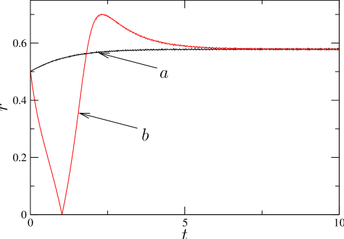
First, we show that the solution deviates from (66) if the analyticity assumtion above does not hold. We perform a direct numerical simulation of the Kuramoto-Sakaguchi model with $N=10^{4}$ oscillators. The frequencies of the oscillators are all different and are chosen to approximate the Lorentzian distribution. For the parameters of coupling we take $\beta=0$, so that $E=\varepsilon$ is real. We perform two runs with the same macroscopic initial conditions for the ensemble, choosing $Y(0)=r(0)e^{i\Theta(0)}=r_{0}=0.5$, but with different initial distribution of phases. Practically, we introduce an auxiliary angle variable $\varsigma$ which attains $N$ values, labelled by index $k$, uniformly distributed between $-\pi$ and $\pi$ (end points are excluded). The frequencies of oscillators are then obtained as $\omega_{k}=\tan\displaystyle\frac{\varsigma_{k}}{2}$ and the initial phases as

$$\phi_{k}=\pm 2\arctan\left[\frac{1-r_{0}}{1+r_{0}}\tan(\varsigma_{k}/2)\right]=\pm 2\arctan\left[\frac{1-r_{0}}{1+r_{0}}\omega_{k}\right]\;,$$ (67)

cf. Eq. (6); here the plus and minus signs correspond to the first and the second run, respectively. Using Eq. (5) and Appendix A we write for the WS variable

$$z(\omega_{k})=e^{i\phi(\omega_{k})}=\frac{r_{0}(1\mp\omega_{k})+1\pm i\omega_{k}}{r_{0}(1\pm i\omega_{k})+1\mp i\omega_{k}}\;.$$ (68)

(Notice that $\rho(\omega_{k})=1$ because we have only one oscillator at each frequency.) Considering the obtained expression as an approximation of a continuous function $z(\omega)$, we find that the latter has a pole at $\omega=\mp i\frac{1+r_{0}}{1-r_{0}}$. Thus, the first case corresponds to an initial condition that is analytic in the upper half-plane, while the second run corresponds to initial conditions that are analytic in lower half-plane. The results are shown in Fig. 4; we see that the transient dynamics of the global mean field heavily depends on the microscopic initial conditions. We emphasize that the result for the first set of initial conditions very well agrees with the solution (66), while for the second set of initial conditions the transient dynamics is essentially different.

Figure 5: Mean field amplitude $r$ as a function of time, for $\varepsilon=3$, $M=10^{4}$. In all simulations initial conditions have been chosen so that $r(0)=0.5$. For $N_{g}=100$ the evolution of the mean field follows Eq. (66), while for smaller group sizes the transient deviates significantly from the OA manifold. In all runs the distribution of the constants $\psi_{a,k}$ inside each group was chosen to be uniform ($q=1$).

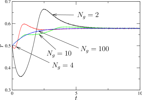
Next, we verify the validity of the theory for hierarchically organized populations, by simulating the same model with $M=10^{4}$ groups of identical elements. All groups have the same size, i.e. $N_{a}=N_{g}$ for all $a=1,\ldots,M$. Again, we always start with the same macroscopic initial conditions for the ensemble, choosing $Y(0)=0.5$. However, the microscopic initial conditions, given by the distribution of the constants of motion $\psi_{a,k}$, differ from run to run. In particular, we introduce a parameter $0<q\leq 1$ that quantifies deviation of the distribution of $\psi_{a,k}$ from a uniform one; the value $q=1$ corresponds to the uniform distribution. In Appendix D we describe how one can choose different microscopic initial conditions while keeping the same macroscopic initial conditions. Here we choose the initial state in such a way, that $z(\omega)$ is analytic in the upper half-plane.

Figure 6: The same as Fig. 5, but for different distributions of constants of motion $\psi_{a,k}$ and fixed group size $N_{g}=200$. Dotted line shows the theoretical asymptotic value of $r$.

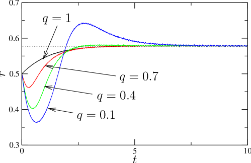
First we analyze the effect of the subpopulation size $N_{g}$ (Fig. 5), taking $q=1$. Theoretically, this effect is described with the help of Eq. (38). The results confirm the theoretical prediction: with increase of $N_{g}$ the transient dynamics tends to the OA manifold and is nicely described by Eq. (66), while for small number of oscillator in a group, the deviations from the OA solution are essential. If there is one oscillator in a group, the OA solution (66) is again valid because here $\rho=1$. The effect of a non-homogeneous distribution of the microscopic constants $\psi_{k,a}$ on the dynamics of the mean field, for a large group sizes, is illustrated in Fig. 6. One can see that the deviations from the OA manifold become larger as this distribution becomes less and less uniform, i.e. if the parameter $q$ deviates from one. The examples of Fig. 4,5,6 illustrate that although the OA ansatz yields a simple closed system of equations, these equations do not describe the dynamics for general initial conditions, but only for a special subset of them.

5.3 Example 2: Two coupled subpopulations

For the next example we concentrate on a model, recently studied by Abrams, Mirollo, Strogatz and Wiley [18]. They considered two identical subpopulations of the same size, i.e. $\omega_{1}=\omega_{2}=\omega$ (without loss of generality we set it to zero) and $N_{1}=N_{2}$, but the coupling within a subgroup differs from the coupling between the subgroups: $\varepsilon_{11}=\varepsilon_{22}=\mu$, $\varepsilon_{12}=\varepsilon_{21}=\nu\neq\mu$, and $\beta_{ab}=\beta$. The equations are:

$$\frac{d\phi_{k}^{(a)}}{dt}=\omega+\mbox{Im}\left[\left(\mu Z_{a}+\nu Z_{b}\right)e^{i(\beta-\phi_{k}^{(a)})}\right]\;,$$ (69)

where $a=1,2$. The WS system (22,23) for this setup reads

$$\frac{dz_{1}}{dt} =\frac{1}{2}H_{1}-\frac{z_{1}^{2}}{2}H_{1}^{*}\;,$$ (70)

$$\frac{d\alpha_{1}}{dt} =\text{Im}(z_{1}^{*}H_{1})\;,$$ (71)

$$\frac{dz_{2}}{dt} =\frac{1}{2}H_{2}-\frac{z_{2}^{2}}{2}H_{2}^{*}\;,$$ (72)

$$\frac{d\alpha_{2}}{dt} =\text{Im}(z_{1}^{*}H_{2})\;,$$ (73)

$$H_{1,2} =(\mu Z_{1,2}+\nu Z_{2,1})e^{i\beta}\;,$$ (74)

and the relation between $Z_{1,2}$ and $z_{1,2}$ is given by Eq. (32). By applying the OA ansatz, i.e. by setting $Z_{1,2}=z_{1,2}$ we obtain a set of equations, originally derived in Ref. [18]. Analyzing these equations, Abrams et al. have obtained an interesting solution where one subpopulation is completely synchronized, $|z_{1}|=1$, while the other one is only partially synchronized, $|z_{2}|<1$. Moreover, this partially synchronous state can be either steady, $z_{2}=const$, or time-periodic, i.e. $z_{2}$ is a periodic function of time. These regimes are called chimera states.

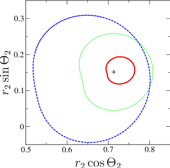
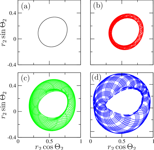
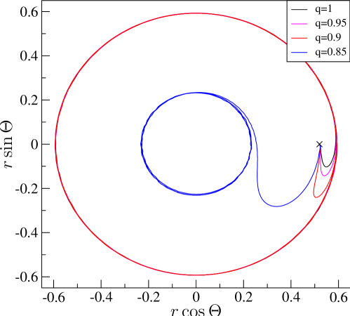
The model of Abrams et al. serves as a good illustration of the usefulness of the above described approach based on the exact WS theory. A complete description of the dynamics for arbitrary initial conditions is given not by the OA equations, but by system (70-74,32). Correspondingly, the additional equations generally lead to an additional time-periodicity for chimera states [40]: a steady-state solution becomes time-periodic (Fig. 7), and a time-periodic state becomes quasiperiodic (Fig. 8). We notice, that in this case the solutions do not evolve towards the OA manifolds, because the distribution of the oscillators’ parameters is not continuous.

Figure 7: (Color online) Simulation of ensemble (69) for $N=64$, $\beta=\pi/2-0.1$, $\mu=0.6$, $\nu=1-\mu=0.4$, and different distributions of the microscopic constants $\psi_{k}^{(2)}$, controlled by the parameter $q$ (see Appendix D). Note that the distribution of constants $\psi_{1,k}$ is irrelevant since the first subpopulation is completely synchronized. The case $q=1$ (marked by plus) corresponds to the OA manifold, here the mean field is constant. For $q=0.9$, $q=0.7$, and $q=0.5$ one observes time-periodic states represented by limit cycles in the complex plane $Z_{2}$ (red bold, green solid, and blue dotted curves, respectively).

Figure 8: The same as in Fig. 7, but for $\mu=0.65$ and $\nu=1-\mu=0.35$. Now on the OA manifold, i.e. for $q=1$, the dynamics is periodic (a), while for more general initial conditions parameterized by $q=0.9$ (b), $q=0.7$ (c), and $q=0.5$ (d) the dynamics is quasiperiodic.

6 Nonlinear mean field coupling

6.1 General nonlinear coupling

Till this moment we restricted our consideration to the case when the force, acting on the oscillator subpopulation $a$, is a linear combination of the local mean fields $Z_{b}$ of all other subpopulations $b$ (see Eq. (52)). We denoted this coupling as linear. Generally, this force can depend on the Daido generalized complex order parameters [32, 34], see Eq. (40). For a general nonlinearity we can expect that $H_{a}$ contains arbitrary combinations of $Z_{b,m}$. However, in a physically reasonable model some restrictions appear.

To discuss this important issue let us first consider an isolated subpopulation, say $a$, and recall that derivation of the phase models of type (1-3) incorporates an averaging over oscillation period (see, e.g., [31]). It means that the mean field forcing $H_{a}$ can include only the terms having the frequency $\approx\omega$, i.e. the terms like

$$Z_{a,1}\;,\qquad Z_{a,m}Z_{a,1-m}\;,\qquad Z_{a,m}Z_{a,l}Z_{a,1-m-l}\;,\ldots\;,$$

where the sum of lower indices is one (we remind that $Z_{-m}=Z_{m}^{*}$). Let us now consider a particular case when the nonlinear mean field coupling is determined by the first order parameter $Z_{a}=Z_{a,1}=r_{a}e^{i\Theta_{a}}$ only. Remarkably, this case corresponds to OA reduced manifold since the latter implies $Z_{m}=Z^{m}$. The forcing then takes the form:

$$H_{a}=h_{1}Z_{a}+h_{3}|Z_{a}|^{2}Z_{a}+h_{5}|Z_{a}|^{4}Z_{a}+\ldots\;.$$ (75)

Denoting $|h_{1}|=\varepsilon$ and $1+\frac{h_{3}}{|h_{1}|}|Z_{a}|^{2}+\frac{h_{5}}{|h_{1}|}|Z_{a}|^{4}+\ldots=A(r_{a},\varepsilon)e^{i\beta(r_{a},\varepsilon)}$ we obtain

$$H_{a}=\varepsilon A(r_{a},\varepsilon)e^{i(\beta(r_{a},\varepsilon)}Z_{a}\;$$ (76)

and

$$\dot{\phi}_{k}^{(a)}=\omega_{a}+\varepsilon A(r_{a},\varepsilon)r\sin\left(\Theta_{a}-\phi_{k}+\beta(r_{a},\varepsilon)\right)\;.$$ (77)

This nonlinear model was suggested and analyzed in [21, 22]; its interesting dynamics is discussed below.

In case when the subpopulation $a$ interacts with the other populations and external fields, Eq. (75) includes additional terms. The terms, describing interaction with other subpopulations can contain any combination of $Z_{b,m}$, with $b=1,\ldots,M$, however, only the terms having the frequency $\approx\omega$ are resonant and therefore essential for the dynamics. This is the consequence of the fact that our basic model (1) is not general but contains only the first harmonics.

6.2 A minimal model of nonlinearly coupled oscillators

Our generalization [21, 22] of the model (60) accounts for a possible nonlinear response of the oscillator to the forcing. It means that the effect of the large force is not just an “up-scaled” effect of the small one, but can be qualitatively different. For a more detailed explanation of this concept, let us consider one oscillator, influenced by a harmonic force with the amplitude $\delta$ and phase $\Theta$ and let the interaction be described by the sine-function, so that the equation for the oscillator’s phase reads:

$$\dot{\phi}=\omega+A\delta\sin(\Theta-\phi_{k}+\beta)\;.$$ (78)

Parameters $A$ and $\beta$ determine the response to the forcing. So, e.g., if $A\cos\beta>0$, the force with a frequency close to $\omega$ results in a stable in-phase synchronization of the oscillator. Consider now an ensemble of identical oscillators, coupled via the mean field. Comparing Eq. (78) with Eq. (61) we identify $\delta$ with $\varepsilon r$ and $\Theta$ with the phase of the mean field. If the oscillators are synchronized, the mean field has the same frequency and the phase as each of them, and if the above condition $A\cos\beta>0$ is fulfilled, then this synchronous regime is stable. Otherwise, if $A\cos\beta<0$, the in-phase synchrony is unstable and the oscillators remain asynchronous, i.e. they have different phases (the frequencies are the same since the oscillators are identical).

Nonlinearity of the coupling means that the parameters in Eq. (78) can depend on the amplitude of the force, $A=A(\delta)$, $\beta=\beta(\delta)$. In this case we can expect interesting dynamics to occur. Suppose the factor $A\cos\beta$ is positive for small $\delta$ but becomes negative when $\delta$ increases and achieves some critical value $\delta_{c}$. Then the synchronous state becomes unstable and the oscillators tend to desynchronize. However, this immediately reduces the mean field, i.e. the amplitude of the forcing $\delta$, and the synchronous state becomes stable again, the oscillators tend to synchronize, what increases the mean field. As a result of the counter-play of these two tendencies, the system settles at the border of stability, exhibiting partially synchronous dynamics: the (identical) oscillators are not synchronized, because synchrony is unstable, but they are also not completely asynchronous, because this state is unstable as well. As a result, the oscillators distribute around the unit circle, forming a bunch. Two different dynamical states appear depending on whether $A$ or $\cos\beta$ becomes negative with an increase of $\delta$. In the former case this bunch remains static in the frame, rotating with the oscillator frequency $\omega_{osc}$. In the latter case, this bunch rotates with respect to the mean field, i.e. the oscillators have frequency that is generally incommensurate with the frequency of the mean field. Furthermore, the bunch can also “breath” so that the mean field is modulated, see [21, 22] for more details.

Let us now take an infinitely large population with a continuous frequency distribution. Consider a particular case of the homogeneous coupling when all oscillators are driven by the same force. Then we should omit the index $a$ in Eq. (75) and substitute there $Z_{a}$ by the global mean field

$$Y=re^{i\Theta}=\int n(\omega)Z(\omega)d\omega\;,\qquad H=\varepsilon A(r,\varepsilon)e^{i\beta(r,\varepsilon)}Y\;$$ (79)

This corresponds to the following microscopic equations

$$\dot{\phi}_{k}=\omega_{k}+\varepsilon A(r,\varepsilon)r\sin\left(\Theta-\phi_{k}+\beta(r,\varepsilon)\right)\;.$$ (80)

Next, we consider the infinitely large system and want to write the corresponding WS equations. We emphasize that in the derivation of Eqs. (63,64) we did not assume that $E=\mbox{const}$; we only used the assumption that the coupling is homogeneous, i.e. that $E$ is independent of the frequency. Hence, we just have to substitute in Eqs. (63,64) $E$ with $\varepsilon A(r,\varepsilon)e^{i(\beta(r,\varepsilon)}$. This yields, together with Eq. (79), a system of integral equations with nonlinear coupling. This full system is still rather difficult to analyse, therefore below we perform, like in Section 5.2 a further simplification allowing us to obtain an analog of Eq. (65).

6.3 Nonlinearly coupled ensemble with the Lorentzian frequency distribution: Theory

In this Section we exploit the general theory to analyze in details the dynamics of ensembles with global nonlinear coupling (see Eqs. (80)) and Lorentzian distribution of frequencies. Looking for the asymptotic solutions we follow the argumentation of Section 4 and consider the reduced dynamics, corresponding to the case $\gamma(\omega)=1$ and, respectively, to the OA reduced manifold. Furthermore, following [23] we consider the Lorentzian distribution of natural frequencies, $n(\omega)=[\pi(\omega^{2}+1)]^{-1}$, and assume that the field $z(\omega)$ is analytic in the upper half-plane. Then, in a way similar to the derivation of Eq. (65), we obtain

$$\frac{dY}{dt}=\left(-1+\frac{\varepsilon A(r,\varepsilon)e^{i\beta(r,\varepsilon)}}{2}\right)Y-\frac{\varepsilon A(r,\varepsilon)e^{i\beta(r,\varepsilon)}}{2}Y^{2}Y^{*}\;.$$ (81)

Below we verify the validity of this equation by numerics; in particular we confirm that the asymptotic solutions are confined to the OA manifold. However, the basins of attraction of these solutions depend on the distribution of the microscopic constants of motion.

Separating the real and imaginary parts of Eq. (81) we obtain equations for the amplitude $r$ and frequency $\Omega$ of the mean field:

$$\displaystyle\frac{dr}{dt} =-r+\frac{\varepsilon A}{2}r(1-r^{2})\cos\beta\;,$$ (82)

$$\displaystyle\frac{d\Theta}{dt} =\Omega=\frac{\varepsilon A}{2}(1+r^{2})\sin\beta\;.$$ (83)

Stability of the asynchronous state $r=0$ of the ensemble is determined by the condition

$$\left.\frac{d\dot{r}}{dr}\right|_{r=0}=-1+\frac{\varepsilon}{2}\left.A\right|_{r=0}\left.\cos\beta\right|_{r=0}=-1+\frac{\varepsilon}{2}A_{0}\cos\beta_{0}<0\;,$$ (84)

what yields the value of the critical coupling

$$\varepsilon_{cr}=\frac{2}{A_{0}\cos\beta_{0}}\;.$$ (85)

For $\varepsilon>\varepsilon_{cr}$ the ensemble exhibits a synchronous state with the mean field amplitude $0<r<1$. The latter is determined from the condition $\dot{r}=0$, which yields the equation

$$\varepsilon(1-r^{2})A(r)\cos\beta(r)=2\;.$$ (86)

If the solution of this equation for particular functions $A$, $\beta$ is found (most likely, numerically), then Eq. (83) provides the frequency of the mean field $\Omega$. Note that the collective oscillation arises with the frequency $\Omega\left|{}_{\varepsilon=\varepsilon_{cr}}\right.=\tan(\beta_{0})$. Below, we illustrate the theory by two particular choices of the amplitude $A(r,\varepsilon)$ and phase $\beta(r,\varepsilon)$ dependencies.

6.4 Nonlinearly coupled ensemble with the Lorentzian frequency distribution: amplitude nonlinearity

First we consider the impact of the amplitude function $A$, by setting $A(r)=\mu-\varepsilon r^{2}$, $\beta=0$. Equations (83) and (85) yield $\Omega=0$ and $\varepsilon_{cr}=2/\mu$. From Eq. (86) we obtain a quadratic equation for $r^{2}$

$$\varepsilon^{2}r^{4}-\varepsilon(\varepsilon+\mu)r^{2}+\varepsilon\mu-2=f(r^{2})=0\;.$$ (87)

It is easy to see that for $\varepsilon>0$ we have $f(\pm\infty)=\infty$, $f(0)=\varepsilon\mu-2$, and $f(1)=-2$. Hence, for $\mu>0$, the solution in the $[0,1]$ interval exists for $\varepsilon>\varepsilon_{cr}=2/\mu$, it is given by

$$r^{2}=\frac{\varepsilon+\mu-\sqrt{(\varepsilon-\mu)^{2}+8}}{2\varepsilon}\;.$$ (88)

The dependence of $r$ on $\varepsilon$ for $\mu=2$, $\varepsilon_{cr}=1$ is shown by bold line in Fig. 9.

Figure 9: Mean field amplitude $r$ as a function of coupling strength $\varepsilon$ for the nonlinearly coupled ensemble with $A=2-\varepsilon r^{2}$ and $\beta=0$. Black bold line: theory. Symbols show simulations of hierarchical ensembles with $M=1000$ groups of $20$ oscillators, for different initial conditions (see text). Red line corresponds to simulation of a population, where all elements have different frequencies, without groups, and with a uniform distribution of $\phi$.

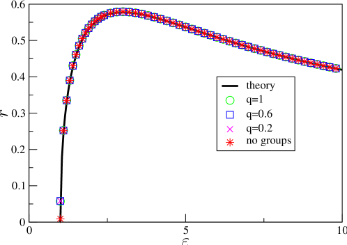
We verify the theory by simulation of ensemble dynamics for $M=1000$ groups of $N_{a}=20$ oscillators. For this goal, we prepare different initial conditions, corresponding to uniform and nonuniform distribution of $\psi_{k,a}$; these distributions are parameterized by parameter $q$, so that $q=1$ and $q<1$ correspond to uniform and non-uniform distributions, respectively (see Appendix D). Next, we simulate the ensemble of $N=10000$ oscillators with different frequencies (in other words, each group contains only one oscillator); in this case we take for initial conditions a nearly uniform distribution of phases $\phi_{k}$. We see, that the results, shown in Fig. 9, demonstrate a good correspondence to the theory.

6.5 Nonlinearly coupled ensemble with the Lorentzian frequency distribution: phase nonlinearity

Now we analyze the effect of the dependence $\beta=\beta(r)$, by setting $A=1$, $\beta=\beta_{0}+\varepsilon^{2}r^{2}$. For the chosen particular function we have $\varepsilon_{cr}=2/\cos\beta_{0}$ and Eq. (86) yields an equation for $r^{2}$:

$$\varepsilon(1-r^{2})\cos(\beta_{0}+\varepsilon^{2}r^{2})-2=f(r^{2})=0\;.$$ (89)

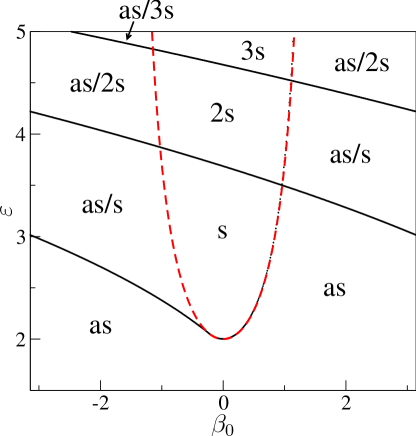
It is easy to see that $f(0)=(\varepsilon-\varepsilon_{cr})\cos\beta_{0}>0$ and $f(1)=-2$, hence there always exist at least one solution. (We remind that $\beta_{0}=\mbox{const}$, $|\beta_{0}|<\pi/2$.) Numerical analysis of Eq. (89) shows that the number of its roots increases with $\varepsilon$. Thus, the system exhibits multistabilty. The corresponding bifurcation diagram in the parameter plane $\beta_{0},\varepsilon$ is shown in Fig. 10.

Figure 10: Multistability in the nonlinearly coupled ensemble with $A=1$, $\beta=\beta_{0}+\varepsilon^{2}r^{2}$. Red dashed line shows critical coupling $\varepsilon_{cr}=2/\cos\beta_{0}$; inside the domain, determined by this curve, the asynchronous state is unstable. Labels as, s, and ns mean asynchrony (the state with $r=0$ is stable), synchrony ($r>0$), and coexistence of $n$ synchronous states, respectively. Label as/ns means coexistence of asynchronous and $n$ synchronous solutions.

Dependencies of the mean field amplitude and frequency on the coupling strength for $\beta_{0}=0$ are shown in Fig. 11.

Figure 11: Illustration of the multistability in the nonlinearly coupled ensemble with $A=1$, $\beta=\beta_{0}+\varepsilon^{2}r^{2}$, for $\beta_{0}=0$. Three branches of the solution of Eq. (89) for the mean field amplitude are shown by different colors in (a). Corresponding solutions for the frequency of the mean field are shown by the same colors in (b). Numerical results (see text for details) are shown by symbols.

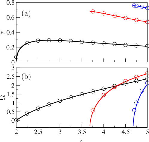
To verify the theory we again perform a direct numerical simulation of an ensemble with $M=5000$ subpopulations of $N_{a}=20$ oscillators each, for $\beta_{0}=0$. The numerical results are shown by symbols in Fig. 11.

Finally, we demonstrate that although the stationary dynamics of the system corresponds to uniform distribution of microscopic constants $\psi$ (i.e., to $q=1$), the transient dynamics does depend on the distribution. In other words, the attractors of the multistable system can be obtained by the simplified theory, see [24] and discussion above, but their basins of attraction depend on the distributions of $\psi$. In numerical experiments, we simulate an ensemble containing $M=5000$ subpopulations of $20$ oscillator each, for $\varepsilon=4.5$, taking $\rho_{0}=0.52$ and different values of $q$. The results shown in Fig. 12 demonstrate that starting from the same macroscopic initial conditions, the system can evolve to different attractors, depending on the microscopic constants.

Figure 12: Evolution of the mean field for same macroscopic initial conditions ($r=0.52$, $\Theta=0$, shown by a cross) but for different distributions of the constants of motions, parameterized by $q$ (see text). Note that both attractors of the system (limit cycles with the radius $\approx 0.23$ and $\approx 0.6$) correspond to the theory, developed under assumption of the uniform distribution of the constants of motion (cf. Fig. 11). However, transient and basins of attraction depend on the distribution of the constants of motion.

7 Conclusions and outlook

The main goal of this paper was to provide a generalization of the powerful Watanabe-Strogatz theory on the heterogeneous populations of phase oscillators. We have formulated the Watanabe-Strogatz equations for a general hierarchically organized ensemble, and have examined limiting cases of infinite populations. Remarkably, there exist two possible thermodynamic limits: in the first one we treat a finite number of infinitely large populations, whereas in the second case we deal with a system with a continuous distribution of parameters, e.g., of frequencies. The derived equations provide an exact reduction of the dynamics; in many cases the problem under consideration becomes low-dimensional. We have analyzed the derived equation in several important cases, including the Kuramoto-Sakaguchi model and the model of two coupled populations with chimera. Noteworthy, the reduced equations are valid both for linear and nonlinear coupling; in the latter case the approach has allowed us to describe multistable synchronous dynamics.

Next, we have thoroughly studied a relation between the Watanabe-Strogatz theory and the recent Ott-Antonsen ansatz and have demonstrated that the latter corresponds to a particular choice of initial conditions for the ensemble. To be exact, the OA approach corresponds to the case when the constants of motion in the Watanabe-Strogatz ansatz are uniformly distributed. Although the Ott-Antonsen equations are much simpler than the full Watanabe-Strogatz system, several examples considered have shown that they provide only asymptotic solutions, whereas the transient dynamics and the basins of attraction of these solutions depend on the choice of initial conditions. (See [47] for another example of nontrivial transient dynamics off the OA manifold.)

Finally, we would like to mention that the approach presented opens new perspectives in analysis of such long-standing problems as finite-size effects and the effects of a common external noise on oscillator ensembles. Also application of it to systems with delayed coupling appears promising.

We thank A. Politi and E. Ott for useful discussions, and E. Ott and S. Strogatz for communicating their works prior to publication. The work was supported by DFG (SFB 555).

Appendix A Watanabe-Strogatz equations in new notations

According to Watanabe and Strogatz [38, 39], the system of $N>3$ identical globally coupled phase oscillators

$$\frac{d\phi_{k}}{dt}=\omega(t)+A(t)\sin(\xi(t)-\phi_{k})=\omega(t)+g(t)\cos\phi_{k}+h(t)\sin\phi_{k}\;$$ (90)

admits a low-dimensional description. For arbitrary functions of time $\omega(t)$, $g(t)$, and $h(t)$, this $N$-dimensional system is completely described by three global variables plus constants of motion $\psi_{k}$, $k=1,\ldots,N$, which obey three additional constraints, so that $N-3$ of them are independent. The “global phases” $\tilde{\Psi}$ and $\tilde{\Phi}$ and the global “amplitude” $0\leq\tilde{\rho}\leq 1$ obey the WS equations

$$\dot{\tilde{\rho}} =-(1-\tilde{\rho}^{2})(g\sin\tilde{\Phi}-h\cos\tilde{\Phi})\;,$$ (91)

$$\tilde{\rho}\dot{\tilde{\Psi}} =-\sqrt{1-\tilde{\rho}^{2}}(g\cos\tilde{\Phi}+h\sin\tilde{\Phi})\;,$$ (92)

$$\tilde{\rho}\dot{\tilde{\Phi}} =-g\cos\tilde{\Phi}-h\sin\tilde{\Phi}\;.$$ (93)

The solution of the original system (90) can be recovered via the following transformation:

$$\tan\left(\frac{\phi_{k}-\tilde{\Phi}}{2}\right)=\sqrt{\frac{1+\tilde{\rho}}{1-\tilde{\rho}}}\tan\left(\frac{\psi_{k}-\tilde{\Psi}}{2}\right)\;.$$ (94)

We perform the variable substitution $\tilde{\rho},\tilde{\Psi},\tilde{\Phi}\to\rho,\Psi,\Phi$ according to

$$\tilde{\rho}=\frac{2\rho}{1+\rho^{2}},\quad\tilde{\Psi}=\Psi+\pi,\quad\tilde{\Phi}=\Phi+\pi\;.$$ (95)

Rewriting the r.h.s. of Eq. (90) as $\omega(t)+\mbox{Im}\left(Z(t)e^{-i\phi_{k}}\right)$ with obvious relations $\mbox{Re}(Z)=-h(t)$, $\mbox{Im}(Z)=g(t)$, we obtain the system of WS equations (7-9) in new variables. The transformation (94) now takes the form

$$\tan\left(\frac{\phi_{k}-\Phi}{2}\right)=\frac{1-\rho}{1+\rho}\tan\left(\frac{\psi_{k}-\Psi}{2}\right)\;.$$ (96)

It is convenient to re-write this transformation in the exponential form, using the following identity:

$$e^{i\alpha} =\frac{1+i\tan(\alpha/2)}{1-i\tan(\alpha/2)}=\frac{\left[1+i\tan(\alpha/2)\right]^{2}}{1+\tan^{2}(\alpha/2)}$$

$$=\cos^{2}\frac{\alpha}{2}\cdot\left(1-\tan^{2}\frac{\alpha}{2}+2i\tan\frac{\alpha}{2}\right)=\cos\alpha+i\sin\alpha\;.$$

With the help of this identity we write:

$$e^{i(\phi_{k}-\Phi)} =\frac{1+i\tan\frac{\phi_{k}-\Phi}{2}}{1-i\tan\frac{\phi_{k}-\Phi}{2}}=\frac{1+i\frac{1-\rho}{1+\rho}\tan\frac{\psi_{k}-\Psi}{2}}{1-i\frac{1-\rho}{1+\rho}\tan\frac{\psi_{k}-\Psi}{2}}$$

$$=\frac{(1+\rho)\cos\frac{\psi_{k}-\Psi}{2}+i(1-\rho)\sin\frac{\psi_{k}-\Psi}{2}}{(1+\rho)\cos\frac{\psi_{k}-\Psi}{2}+i(\rho-1)\sin\frac{\psi_{k}-\Psi}{2}}$$

$$=\frac{\rho e^{-i(\psi_{k}-\Psi)/2}+e^{i(\psi_{k}-\Psi)/2}}{\rho e^{i(\psi_{k}-\Psi)/2}+e^{-i(\psi_{k}-\Psi)/2}}\;,$$

what yields the desired transformation (5).

Appendix B Dynamics of WS variables in an external field

Here we present the exact solution of Eqs. (19-21) for the case $|\omega-\nu|>H_{0}$. The system has one steady state $\Delta_{0}=0$ and

$$\rho_{0}=\begin{cases}-(\omega-\nu)H_{0}^{-1}+\sqrt{(\omega-\nu)^{2}H_{0}^{-2}-1}&\mbox{for~{}}(\omega-\nu)>H_{0}\;,\\[4.30554pt] -(\omega-\nu)H_{0}^{-1}-\sqrt{(\omega-\nu)^{2}H_{0}^{-2}-1}&\mbox{for~{}}(\omega-\nu)<-H_{0}\;.\end{cases}$$ (97)

Equation (21) then yields

$$\dot{\alpha}=\omega-\nu-H_{0}\rho_{0}=2(\omega-\nu)\mp\sqrt{(\omega-\nu)^{2}-H_{0}^{2}}\;.$$

Hence, $\Psi$ rotates with the frequency

$$\kappa=3\nu-2\omega\pm\sqrt{(\omega-\nu)^{2}-H_{0}^{2}}\;.$$ (98)

Consider now solution with $\rho\neq\rho_{0}$ and $\Delta\neq\Delta_{0}$. Introducing new variables $u=\rho\cos\Delta$, $v=\rho\sin\Delta$, we write the first two equations as

$$\dot{u} =-(\omega-\nu)u-H_{0}uv\;,$$ (99)

$$\dot{v} =(\omega-\nu)u+\frac{H_{0}}{2}(1+u^{2}-v^{2})\;,$$

with $v_{0}=0$ and $u_{0}=\rho_{0}$. Introducing $w=u-u_{0}$ we rewrite (99) as

$$\dot{w} =-(\omega-\nu+H_{0}u_{0})v-H_{0}wv\;,$$ (100)

$$\dot{v} =(\omega-\nu+H_{0}u_{0})w+\frac{H_{0}}{2}(w^{2}-v^{2})\;.$$

Using an ansatz $p=v(v^{2}+w^{2})^{-1}$, $q=w(v^{2}+w^{2})^{-1}$ and denoting

$$\kappa=\omega-\nu+H_{0}u_{0}=\mp\sqrt{(\omega-\nu)^{2}-H_{0}^{2}}$$ (101)

we simplify the equations to

$$\dot{p} =\kappa q+\frac{H_{0}}{2}\;,$$ (102)

$$\dot{q} =-\kappa p\;.$$

The solution of the latter system is

$$p =A\cos(\kappa(t-t_{0}))\;,$$ (103)

$$q =A\sin(\kappa(t-t_{0}))-\frac{H_{0}}{2\kappa}\;.$$

Transforming back to $u,v$ we obtain

$$u=\rho\cos\Delta =x_{0}+\frac{A\sin(\kappa(t-t_{0}))-\frac{H_{0}}{2\kappa}}{A^{2}+\frac{H_{0}^{2}}{4\kappa^{2}}-\frac{AH_{0}}{\kappa\sin(\kappa(t-t_{0}))}}\;,$$ (104)

$$v=\rho\sin\Delta =\frac{A\cos(\kappa(t-t_{0}))}{A^{2}+\frac{H_{0}^{2}}{4\kappa^{2}}-\frac{AH_{0}}{\kappa\sin(\kappa(t-t_{0}))}}\;.$$

In these variables Eq. (21) takes the form

$$\dot{\alpha}=\omega-\nu-H_{0}u\;$$ (105)

and is readily solved by substitution of (104) and integration. As a result we obtain a quasiperiodic solution: variables $\rho$ and $\Delta$ oscillate with the frequency $\kappa$ (it means that $\Phi$ has the frequency $\kappa+\nu$) and $\Psi=\Phi-\alpha$ possesses an additional frequency, found via integration of (105).

Appendix C Variable transformation for continuity equation

We perform transformation of variables in Eq. (27), using Eq. (28):

$$\begin{array}[]{ll}0&=\displaystyle\frac{\partial w}{\partial t}+\frac{\partial}{\partial\phi}(wv)=\displaystyle\frac{\partial w}{\partial\tau}\displaystyle\frac{\partial\tau}{\partial t}+\displaystyle\frac{\partial w}{\partial\psi}\displaystyle\frac{\partial\psi}{\partial t}+\frac{\partial}{\partial\psi}(wv)\frac{\partial\psi}{\partial\phi}\\[17.22217pt] &=\displaystyle\frac{\partial}{\partial\tau}\left(\sigma\displaystyle\frac{\partial\psi}{\partial\phi}\right)+\displaystyle\frac{\partial}{\partial\psi}\left(\sigma\displaystyle\frac{\partial\psi}{\partial\phi}\right)\cdot\displaystyle\frac{\partial\psi}{\partial t}+\left[\frac{\partial}{\partial\psi}\left(\sigma\displaystyle\frac{\partial\psi}{\partial\phi}\right)v+\left(\sigma\displaystyle\frac{\partial\psi}{\partial\phi}\right)\frac{\partial v}{\partial\psi}\right]\frac{\partial\psi}{\partial\phi}\\[17.22217pt] &=\displaystyle\frac{\partial\sigma}{\partial\tau}\displaystyle\frac{\partial\psi}{\partial\phi}+\sigma\displaystyle\frac{\partial}{\partial\tau}\left(\displaystyle\frac{\partial\psi}{\partial\phi}\right)+\left[\displaystyle\frac{\partial\sigma}{\partial\psi}\displaystyle\frac{\partial\psi}{\partial\phi}+\sigma\displaystyle\frac{\partial}{\partial\psi}\left(\displaystyle\frac{\partial\psi}{\partial\phi}\right)\right]\displaystyle\frac{\partial\psi}{\partial t}\\[17.22217pt] &+\left\{\left[\displaystyle\frac{\partial\sigma}{\partial\psi}\displaystyle\frac{\partial\psi}{\partial\phi}+\sigma\displaystyle\frac{\partial}{\partial\psi}\left(\displaystyle\frac{\partial\psi}{\partial\phi}\right)\right]v+\sigma\displaystyle\frac{\partial\psi}{\partial\phi}\displaystyle\frac{\partial v}{\partial\psi}\right\}\displaystyle\frac{\partial\psi}{\partial\phi}\\[17.22217pt] &=\displaystyle\frac{\partial\sigma}{\partial\tau}\displaystyle\frac{\partial\psi}{\partial\phi}+\sigma\left\{\displaystyle\frac{\partial}{\partial\tau}\left(\displaystyle\frac{\partial\psi}{\partial\phi}\right)+\displaystyle\frac{\partial}{\partial\psi}\left(\displaystyle\frac{\partial\psi}{\partial\phi}\right)\left(\displaystyle\frac{\partial\psi}{\partial t}+v\displaystyle\frac{\partial\psi}{\partial\phi}\right)+\left(\displaystyle\frac{\partial\psi}{\partial\phi}\right)^{2}\displaystyle\frac{\partial v}{\partial\psi}\right\}\\[17.22217pt] &+\displaystyle\frac{\partial\sigma}{\partial\psi}\left\{\displaystyle\frac{\partial\psi}{\partial\phi}\left(\displaystyle\frac{\partial\psi}{\partial t}+v\displaystyle\frac{\partial\psi}{\partial\phi}\right)\right\}\;.\end{array}$$ (106)

Let us demonstrate that the coefficients at $\sigma$ and $\displaystyle\frac{\partial\sigma}{\partial\psi}$ vanish if $\rho$, $\Phi$, and $\Psi$ obey the WS equations. For this goal we first compute $\displaystyle\frac{\partial\psi}{\partial t}+v\displaystyle\frac{\partial\psi}{\partial\phi}$. It is convenient to use the notations $f=e^{i(\phi-\Phi)}$, $c=e^{i(\psi-\Psi)}$. Resolving Eq. (5) with respect to $\psi$, we obtain

$$\psi=\Psi-i\ln(f-\rho)+i\ln(1-\rho f)\;.$$ (107)

Taking the derivative and re-arranging the terms, we obtain

$$\frac{\partial\psi}{\partial t}(\phi)=\dot{\Psi}-f\frac{1-\rho^{2}}{(f-\rho)(1-f\rho)}\dot{\Phi}+i\frac{1-f^{2}}{(f-\rho)(1-f\rho)}\dot{\rho}\;.$$ (108)

Using $e^{-i\phi}=e^{-i\Phi}/f=e^{-i\Phi}f^{*}$, we obtain in new variables:

$$v=\omega+\mbox{Im}\left[He^{-i\Phi}f^{*}\right]\;.$$ (109)

Next, from Eq. (107) we compute, using $\displaystyle\frac{\partial f}{\partial\phi}=if$:

$$\frac{\partial\psi}{\partial\phi}(\phi)=\frac{(1-\rho^{2})f}{(f-\rho)(1-\rho f)}\;.$$ (110)

Substituting into Eq. (108) the derivatives via the r.h.s. of the WS equations and using Eqs. (109,110), we obtain after tedious but straightforward algebra

$$\frac{\partial\psi}{\partial t}+v\displaystyle\frac{\partial\psi}{\partial\phi}=0\;.$$ (111)

Hence the coefficient at $\displaystyle\frac{\partial\sigma}{\partial\psi}=0$ and the coefficient at $\sigma$ reduces to

$$\frac{\partial}{\partial\tau}\left(\displaystyle\frac{\partial\psi}{\partial\phi}\right)+\left(\displaystyle\frac{\partial\psi}{\partial\phi}\right)^{2}\displaystyle\frac{\partial v}{\partial\psi}=Q\;.$$

To compute $Q$, we first substitute in Eq. (110) $f=\displaystyle\frac{\rho+c}{\rho c+1}$ from Eq. (5) and obtain, after straightforward manipulations,

$$\frac{\partial\psi}{\partial\phi}(\psi)=\frac{(\rho+c)(\rho+c^{*})}{1-\rho^{2}}=\frac{\rho c+\rho c^{*}+2}{1-\rho^{2}}-1\;.$$ (112)

Derivation with respect to time yields

$$\frac{\partial}{\partial\tau}\left(\displaystyle\frac{\partial\psi}{\partial\phi}\right)=\displaystyle\frac{\partial}{\partial t}\left(\displaystyle\frac{\partial\psi}{\partial\phi}\right)=\frac{i\rho(c^{*}-c)}{1-\rho^{2}}\dot{\Psi}+\frac{(1+\rho^{2})(c+c^{*})+4\rho}{(1-\rho^{2})^{2}}\dot{\rho}\;.$$ (113)

Here we used $\displaystyle\frac{\partial c}{\partial t}=-ic\dot{\Psi}$, $\displaystyle\frac{\partial c^{*}}{\partial t}=ic^{*}\dot{\Psi}$. Next, we compute

$$\frac{\partial v}{\partial\psi}=\mbox{Im}\left[He^{-i\Phi}\displaystyle\frac{\partial}{\partial\psi}\frac{\rho c+1}{\rho+c}\right]=(\rho^{2}-1)\mbox{Re}\left[\displaystyle\frac{cHe^{-i\Phi}}{(\rho+c)^{2}}\right]\;.$$ (114)

Using the obtained expressions (112-114), we show, after tedious but straightforward manipulations, that $Q=0$ if $\dot{\Psi}$ and $\dot{\rho}$ obey the WS equations.

Thus, we demonstrate that the r.h.s. of the continuity equation Eq. (106) simplifies to $\displaystyle\frac{\partial\sigma}{\partial\tau}\displaystyle\frac{\partial\psi}{\partial\phi}$ and is therefore valid if $\sigma(\omega,\psi)$ is a stationary distribution.

Appendix D Choice of initial conditions for simulation of hierarchical populations

Our goal is to choose different microscopic initial conditions, i.e. initial values for oscillator phases, but keep the same macroscopic initial conditions, i.e. the amplitude of the mean field. For this goal we proceed as follows. For each subpopulation with the frequency $\omega_{a}$ we take $\psi_{a}$ uniformly distributed along the arcs $[(1-q)\frac{\pi}{2},(1+q)\frac{\pi}{2}]$ and $[-(1+q)\frac{\pi}{2}],-(1-q)\frac{\pi}{2}]$, as shown in Fig. 13. Here $0<q\leq 1$ is a parameter quantifying deviation of the distribution from a uniform one; $q=1$ corresponds do a uniform distribution, with $q\to 0$ the distribution collapses to two points. For this construction, the subpopulation $N_{a}$ should be an even number. Note that this choice of $\psi_{a,k}$ satisfies constraints (12) and $\sum\psi_{a,k}=0$. The initial values of the oscillator phases $\phi_{a,k}(0)$ are obtained from $\psi_{a,k}$ according to Eq. (96).

Figure 13: Illustration of the special choice of the constants of motion $\psi_{k}$, here for $q=0.8$ and $N_{a}=10$. The points are distributed along two arcs of length $q\pi$ each; angle $\alpha=\displaystyle\frac{\pi}{2}(1-q)$, angle $\beta=\displaystyle\frac{q\pi}{N_{a}}$.

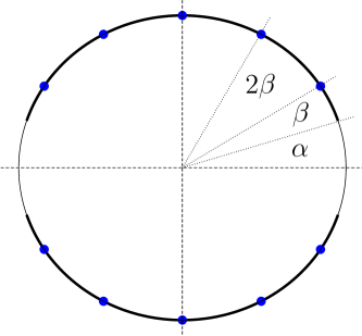
Now we show that with a special choice of the initial values of the WS variables we can ensure the same initial value of the mean field, independently of the parameter $q$. These special values are $\Phi_{a}=0$, $\rho_{a}=\rho_{0}$, and $\Psi_{a}=\frac{2\pi}{M}a$. In order to compute the initial value of the Kuramoto mean field $Y(0)=r_{0}e^{i\Theta_{0}}$ we write the discrete version of Eq. (49) for $t=0$:

$$r_{0}e^{i\Theta_{0}} =\rho_{0}\sum_{a=1}^{M}n_{a}\gamma_{a}$$

$$=\rho_{0}\left(\sum_{a=1}^{M}n_{a}+(1-\rho_{0}^{-2})\sum_{a=1}^{M}n_{a}\sum_{l=2}^{\infty}C_{l}(-\rho_{0})^{l}e^{-i\frac{2\pi al}{M}}\right)$$

$$=\rho_{0}\;,$$

with account that all groups are of equal size, $n_{a}=n$. Thus, taking different values of the parameter $q$ and fixing other parameters we obtain the same macroscopic initial conditions (i.e. for the mean field), whereas the initial conditions for individual oscillators are different.

References

- [1] K. Wiesenfeld and J. W. Swift. Averaged equations for Josephson junction series arrays. Phys. Rev. E, 51(2):1020–1025, 1995.
- [2] A. F. Glova. Phase locking of optically coupled lasers. Quantum Electronics, 33(4):283–306, 2003.
- [3] I.Z. Kiss, Y. Zhai, and J.L. Hudson. Emerging coherence in a population of chemical oscillators. Science, 296:1676–1678, 2002.
- [4] S. H. Strogatz, D. M. Abrams, A. McRobie, B. Eckhardt, and E. Ott. Theoretical mechanics: Crowd synchrony on the Millennium Bridge. Nature, 438:43–44, 2005.
- [5] B. Eckhardt, E. Ott, S. H. Strogatz, D. M. Abrams, and A. McRobie. Modeling walker synchronization on the Millennium Bridge. Phys. Rev. E, 75:021110, 2007.
- [6] Z. Néda, E. Ravasz, Y. Brechet, T. Vicsek, and A.-L. Barabási. Tumultuous applause can transform itself into waves of synchronized clapping. Nature, 403(6772):849–850, 2000.
- [7] P. Richard, B. M. Bakker, B. Teusink, K. Van Dam, and H. V. Westerhoff. Acetaldehyde mediates the synchronization of sustained glycolytic oscillations in population of yeast cells. Eur. J. Biochem., 235:238–241, 1996.
- [8] S. Dano, P. G. Sorensen, and F. Hynne. Sustained oscillations in living cells. Nature, 402(6759):320–322, 1999.
- [9] D. Gonze, N. Markadieu, and A. Goldbeter. Selection of in-phase or out-of-phase synchronization in a model based on global coupling of cells undergoing metabolic oscillations. CHAOS, 18(3):037127, SEP 2008.
- [10] D. Golomb, D. Hansel, and G. Mato. Mechanisms of synchrony of neural activity in large networks. In F. Moss and S. Gielen, editors, Neuro-informatics and Neural Modeling, volume 4 of Handbook of Biological Physics, pages 887–968. Elsevier, Amsterdam, 2001.
- [11] H. Sakaguchi. Cooperative phenomena in coupled oscillator systems under external fields. Prog. Theor. Phys., 79(1):39–46, 1988.
- [12] T. M. Antonsen, Jr., R. T. Faghih, M. Girvan, E. Ott, and J. Platig. External periodic driving of large systems of globally coupled phase oscillators. Chaos, 18(3):037112, 2008.
- [13] P. A. Tass. Phase Resetting in Medicine and Biology. Stochastic Modelling and Data Analysis. Springer-Verlag, Berlin, 1999.
- [14] M. Rosenblum and A. Pikovsky. Controlling synchronization in an ensemble of globally coupled oscillators. Phys. Rev. Lett., 92(11):114102, 2004.
- [15] M. Rosenblum and A. Pikovsky. Delayed feedback control of collective synchrony: An approach to suppression of pathological brain rhythms. Phys. Rev. E, 70:041904, 2004.
- [16] L. M. Childs and S. H. Strogatz. Stability diagram for the forced Kuramoto model. Chaos: An Interdisciplinary Journal of Nonlinear Science, 18(4):043128, 2008.
- [17] E. A. Martens, E. Barreto, S. H. Strogatz, E. Ott, P. So, and T. M. Antonsen. Exact results for the Kuramoto model with a bimodal frequency distribution. Physical Review E, 79(2):026204, 2009.
- [18] D. M. Abrams, R. Mirollo, S. H. Strogatz, and D. A. Wiley. Solvable model for chimera states of coupled oscillators. Phys. Rev. Lett., 101:084103, 2008.
- [19] O. E. Omel’chenko, Yu. L. Maistrenko, and P. A. Tass. Chimera states: The natural link between coherence and incoherence. Physical Review Letters, 100(4):044105, 2008.
- [20] C. R. Laing. The dynamics of chimera states in heterogeneous Kuramoto networks. Physica D: Nonlinear Phenomena, 238(16):1569 – 1588, 2009.
- [21] M. Rosenblum and A. Pikovsky. Self-organized quasiperiodicity in oscillator ensembles with global nonlinear coupling. Phys. Rev. Lett., 98:064101, 2007.
- [22] A. Pikovsky and M. Rosenblum. Self-organized partially synchronous dynamics in populations of nonlinearly coupled oscillators. Physica D, 238(1):27–37, 2009.
- [23] E. Ott and Th. M. Antonsen. Low dimensional behavior of large systems of globally coupled oscillators. CHAOS, 18(3):037113, 2008.
- [24] E. Ott and Th. M. Antonsen. Long time evolution of phase oscillator systems. CHAOS, 19(2):023117, 2009.
- [25] D. Paźo. Thermodynamic limit of the first-order phase transition in the Kuramoto model. Phys. Rev. E, 72(4, Part 2):046211, OCT 2005.
- [26] D. Paźo and E. Montbrió. Existence of hysteresis in the Kuramoto model with bimodal frequency distributions, 2009. Phys. Rev. E, 80: 046215, 2009.
- [27] H. Kori and Y. Kuramoto. Slow switching in globally coupled oscillators: robustness and occurrence through delayed coupling. Phys. Rev. E, 63:046214, 2001.
- [28] Z. Liu, Y.-C. Lai, and F. C. Hoppensteadt. Phase clustering and transition to phase synchronization in a large number of coupled nonlinear oscillators. Phys. Rev. E, 63(5):055201, 2001.
- [29] Yu. Maistrenko, O. Popovych, O. Burylko, and P. A. Tass. Mechanism of desynchronization in the finite-dimensional Kuramoto model. Phys. Rev. Lett., 93(8):084102, Aug 2004.
- [30] Y. Kuramoto. Self-entrainment of a population of coupled nonlinear oscillators. In H. Araki, editor, International Symposium on Mathematical Problems in Theoretical Physics, page 420, New York, 1975. Springer Lecture Notes Phys., v. 39.
- [31] Y. Kuramoto. Chemical Oscillations, Waves and Turbulence. Springer, Berlin, 1984.
- [32] H. Daido. Order function and macroscopic mutual entrainment in uniformly coupled limit-cycle oscillators. Prog. Theor. Phys., 88(6):1213–1218, 1992.
- [33] H. Daido. Critical conditions of macroscopic mutual entrainment in uniformly coupled limit-cycle oscillators. Prog. Theor. Phys., 89(4):929–934, 1993.
- [34] H. Daido. Onset of cooperative entrainment in limit-cycle oscillators with uniform all-to-all interactions: Bifurcation of the order function. Physica D, 91:24–66, 1996.
- [35] A. Pikovsky, M. Rosenblum, and J. Kurths. Synchronization. A Universal Concept in Nonlinear Sciences. Cambridge University Press, Cambridge, 2001.
- [36] J. A. Acebron, L. L. Bonilla, C. J. Perez Vicente, F. Ritort, and R. Spigler. The Kuramoto model: A simple paradigm for synchronization phenomena. Rev. Mod. Phys., 77(1):137–175, 2005.
- [37] S. H. Strogatz. From Kuramoto to Crawford: Exploring the onset of synchronization in populations of coupled oscillators. Physica D, 143(1-4):1–20, 2000.
- [38] S. Watanabe and S. H. Strogatz. Integrability of a globally coupled oscillator array. Phys. Rev. Lett., 70(16):2391–2394, 1993.
- [39] S. Watanabe and S. H. Strogatz. Constants of motion for superconducting Josephson arrays. Physica D, 74:197–253, 1994.
- [40] A. Pikovsky and M. Rosenblum. Partially integrable dynamics of hierarchical populations of coupled oscillators. Phys. Rev. Lett., 101:264103, 2008.
- [41] S. A. Marvel, R. E. Mirollo, and S. H. Strogatz. Phase oscillators with global sinusoidal coupling evolve by Mobius group action. arXiv:0904.1680, 2009. (CHAOS, submitted).
- [42] E. Barreto, B. Hunt, E. Ott, and P. So. Synchronization in networks of networks: The onset of coherent collective behavior in systems of interacting populations of heterogeneous oscillators. Phys. Rev. E, 77:036107, 2008.
- [43] W. S. Lee, E. Ott, Th. M. Antonsen. Large coupled oscillator systems with heterogeneous interaction delays. Phys. Rev. Lett., 103:044101, 2009.
- [44] M. M. Abdulrehem, E. Ott. Low dimensional description of pedestrian-induced oscillation of the Millennium Bridge. CHAOS, 19(1):013129, 2009.
- [45] H. Daido. Multi-branch entrainment and multi-peaked order-functions in a phase model of limit-cycle oscillators with uniform all-to-all coupling. J. Phys. A: Math. Gen., 28:L151–L157, 1995.
- [46] H. Sakaguchi and Y. Kuramoto. A soluble active rotator model showing phase transition via mutual entrainment. Prog. Theor. Phys., 76(3):576–581, 1986.
- [47] E. Ott, J. H. Platig, Th. M. Antonsen, and M. Girvan. Echo phenomena in large systems of coupled oscillators. CHAOS, 18(3):037115, 2008.