Measuring galaxy segregation using the mark connection function

Abstract

Context. The clustering properties of galaxies belonging to different luminosity ranges or having different morphological types are different. These characteristics or ‘marks’ permit to understand the galaxy catalogs that carry all this information as realizations of marked point processes. Many attempts have been presented to quantify the dependence of the clustering of galaxies on their inner properties.

Aims. The present paper summarizes methods on spatial marked statistics used in cosmology to disentangle luminosity, colour or morphological segregation and introduces a new one in this context, the mark connection function.

Methods. The methods used here are the partial correlation functions, including the cross-correlation function, the normalised mark correlation function, the mark variogram and the mark connection function. All these methods are applied to a volume-limited sample drawn from the 2dFGRS, using the spectral type $\eta$ as the mark.

Results. We show the virtues of each method to provide information about the clustering properties of each population, the dependence of the clustering on the marks, the similarity of the marks as a function of the pair distances, and the way to characterise the spatial correlation between the marks. We demonstrate by means of these statistics that passive galaxies exhibit stronger spatial correlation than active galaxies at small scales ($r\lesssim 20$ $h^{-1}$ Mpc), and that the price galaxies have to pay to be close together is having smaller values of the assigned marks, which means in our case being more passive. Through the mark connection function we quantify the relative positioning of different types of galaxies within the overall clustering pattern.

Conclusions. The different marked statistics provide different information about the clustering properties of each population. Different aspects of the segregation are encapsulated by each measure, being the new one introduced here –the mark connection function– particularly useful for understanding the spatial correlation between the marks.

1 Introduction

Galaxies of different morphological types show different clustering properties. It is well known, for example, that elliptical galaxies are preferentially found in high density environments, such as the centres of rich galaxy clusters (Dressler 1980), while the dominant population of the field are mainly spiral galaxies (Davis & Geller 1976; Dressler 1980). Second order characteristics as the two point correlation function have been used to quantify the clustering of galaxies with different morphologies, different spectral characteristics, different colours or belonging to different luminosity ranges (Phillipps & Shanks 1987; Hamilton 1988; Davis et al. 1988; Loveday et al. 1995; Hermit et al. 1996; Guzzo et al. 1997). Bright galaxies show stronger spatial correlation than faint ones. Other clustering measures have been also used to quantify the luminosity or morphological segregation: multifractals (Domínguez-Tenreiro & Martínez 1989; Domínguez-Tenreiro et al. 1994), void probability functions (Vogeley et al. 1991; Croton et al. 2004), distributions of the distances to the nearest neighbours (Salzer et al. 1990), etc.

The two-point correlation function $\xi(r)$ measures the excess probability of finding a neighbour at a distance $r$ from a given galaxy when compared with that probability for a homogeneous Poisson process. Morphological segregation is encapsulated by the behaviour of $\xi(r)$ when it is calculated separately for different populations of galaxies. Elliptical galaxies show at small scales a correlation function with steeper slopes and larger amplitudes than spirals (Loveday et al. 1995). A recent analysis of the Two Degree Field Galaxy Redshift Survey (2dFGRS) has shown the same trend when comparing populations for different spectral types, being the two-point correlation function steeper for passive galaxies than for active galaxies (Madgwick et al. 2003). Also, Zehavi et al. (2002) have analysed the distribution of red and blue galaxies in the Sloan Digital Sky Survey (SDSS) by means of the projected correlation funcion $w_{p}(r_{p})$ showing that red galaxies display a more prominent and steeper real-space correlation function than blue galaxies do.

The galaxy distribution can be considered a realisation of a point process. However, in many situations, each galaxy (point in the process) carries additional information regarding a given characteristic (e.g. morphological type) or a given numerical value that measures a given galaxy property: luminosity, colour, spectral type. If we attach this characteristic (mark) to the point in the process, we end up at a marked point process, as it is called in mainstream spatial statistics (Stoyan & Stoyan 1994; Martínez & Saar 2002; Illian et al. 2008).

In this work, we compare different statistical methods for the study of the marked galaxy distribution. We also introduce – for the first time in this context – the mark connection function. We illustrate the usefulness of these methods by applying them to a volume-limited sample drawn from the 2dFGRS with marks given by the galaxy spectral type. In Section 2, we describe the sample and the marks assigned to the galaxies. In Section 3 we describe the different statistical methods considered, and in Section 4 we show the results of applying them to our galaxy sample. In the conclusions, we stress the capabilities of the mark connection function to characterise the spatial correlation between the marks.

2 The 2dFGRS subsamples

To illustrate the different mark clustering measures, we used a nearly volume-limited sample drawn from the 2dFGRS and prepared by the 2dF team (Croton et al. 2004). It contains galaxies with absolute magnitudes in the range $-20<M_{b_{J}}<-19$ at redshifts $z<0.13$. In order to avoid the effects of complicated boundaries while using a simple estimator, we selected galaxies inside a rectangular parallelepiped inscribed in the North slice of 2dFGRS. The final sample used contains $N=7741$ galaxies and covers a volume of $V\sim 10^{6}$ ($h^{-1}$ Mpc)³ where $h$ is the Hubble constant in units of 100 km s^-1 Mpc^-1 .

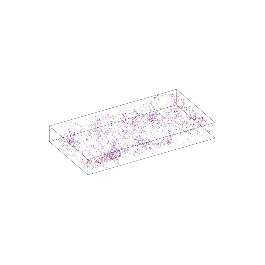
We characterized the galaxies in the sample using the spectral classification parameter $\eta$ (Madgwick et al. 2002). Lower values of $\eta$ correspond to more passive or ‘early-type’ galaxies, while larger values correspond to active or ‘late-type’ ones. In order to avoid negative values of the marks, we defined the mark used as $m=\eta+10$. This shift does not affect our conclusions. Based on this $\eta$ parameter, we divided our sample in two populations, following Madgwick et al. (2003): population ‘1’ (passive galaxies) with $\eta\leq-1.4$, and population ‘2’ (active galaxies) with $\eta>-1.4$. These subsamples contain $N_{1}=3828$ and $N_{2}=3913$ galaxies, respectively. We show the sample used in Fig. 1.

Figure 1: Tridimensional plot of the galaxy sample used. Red dots correspond to early-type galaxies (population ‘1’), and blue dots to late-type galaxies (population ‘2’). The parallelepiped dimensions are $254\times 133\times 31$ $h^{-1}$ Mpc.

In order to test the existence of mark segregation, we compared the results obtained for the different statistics with random relabelling simulations. In these, we keep the original positions of galaxies, but redistribute the marks randomly among them. This corresponds to a model in which clustering is independent of the mark, or spectral type, of the galaxies. We simulated $n=200$ realizations using the random relabelling method, and obtained their maximum and minimum values as function of distance $r$ for each statistic. Deviations of the observed statistics from this range of values correspond to rejection of the mark-independent clustering model at a pointwise significance of $1-\frac{2}{n+1}\simeq 99\%$ (Illian et al. 2008).

3 Clustering analysis methods

Recently, the clustering dependence on luminosity, colour or morphology has been analysed by means of the marked clustering statistics, that allow to study the galaxy clustering as a function of their properties, and moreover this approach provides us with different measures of the correlation between the galaxy properties and the environment (Skibba et al. 2009). The galaxy distribution is interpreted as a realisation of a marked point process $X^{M}=\{(\@vec{x}_{i},m_{i})\}$, where the mark $m_{i}$ denotes an intrinsic property of the galaxy at position $\@vec{x}_{i}$. The mark can be the luminosity, the spectral type, the colour, etc. In general, today galaxy catalogues provide quantitative marks ranging in a continuous interval rather than just a discrete characteristic like a galaxy being spiral or elliptical. In any case, we shall also show how to use interesting second-order measures to disentangle clustering dependent characteristics of two populations by dividing the sample in two parts using a significant value of the mark as threshold $m_{\rm thres}$ and separating the two populations according to the value of the mark: population ‘1’ with $m_{i}\leq m_{\rm thres}$ and population ‘2’ with $m_{i}\geq m_{\rm thres}$.

We describe below the different methods we used to obtain information about galaxy clustering segregation. They are the classical partial correlation functions (for two discrete populations), the normalized mark correlation function and the mark variogram (based on the use of continuous marks), and finally the mark connection function (based on the use of discrete marks).

We computed the different statistics based on the estimation of the second-order intensity function for the unmarked point process ($\lambda_{2}(r)$) presented in Stoyan & Stoyan (1994), Pons-Bordería et al. (1999), and Illian et al. (2008),

$$\hat{\lambda}_{2}(r)=\frac{1}{4\pi r^{2}}\sum_{i=1}^{N}\sum\limits_{j=1\atop j\neq i}^{N}\frac{k(r-|\@vec{x}_{i}-\@vec{x}_{j}|)}{V(W\cap W_{\@vec{x}_{i}-\@vec{x}_{j}})}\,,$$ (1)

where $\@vec{x}_{i}$ are the positions of the points, $k(\cdot)$ is a kernel function, and $V(W\cap W_{\@vec{r}})$ is the volume of the window (the parallelepiped in our case) intersected with a version of itself shifted by the vector $\@vec{r}$ (see Fig. 1 in Pons-Bordería et al. 1999).

In all our calculations we used the Epanechnikov kernel,

$$k(x)=\left\{\begin{array}[]{ll}\frac{3}{4w}\left(1-\frac{x^{2}}{w^{2}}\right)&\mbox{for}\,-w\leq x\leq w\\ 0&\mbox{otherwise}\end{array}\right.$$

with width $w=1$ $h^{-1}$ Mpc, and sampled the different functions with a step in $r$ of 0.5 $h^{-1}$ Mpc. This compact kernel is very well suited for correlation analysis (Pons-Bordería et al. 1999). We note, however, that the choice of a given kernel is not crucial, while the choice of the bandwith, $w$, is more important and plays the role of the binning in the standard calculation of correlation functions, where a top-hat kernel is typically used as default.

3.1 Partial two-point correlation functions

In the standard clustering analysis of the galaxy distribution, the two-point correlation function, $\xi(r)$, measures the clustering in excess ($\xi(r)>0$) or in defect ($\xi(r)<0$) relative to a Poisson distribution, for which $\xi(r)=0$. Whenever we want to compare the clustering properties of different populations of galaxies encapsulated by their spatial correlations, we can consider the correlation function restricted to a given population, which are called partial correlation functions. In fact, for two populations of interest, one can consider three partial two-point correlation functions, namely $\xi_{11}(r)$, $\xi_{22}(r)$, and $\xi_{12}(r)$. The first two are those mentioned above for types 1 and 2, while the cross-correlation function (Peebles 1980) $\xi_{12}(r)$ measures the excess probability of finding a neighbour of type ‘1’ at distance $r$ from a given galaxy of type ‘2’, or vice versa.

Based on equation (1), the partial two-point correlation functions were estimated as

$$\hat{\xi}_{ij}(r)=\frac{1}{4\pi r^{2}\hat{n}_{i}\hat{n}_{j}}\sum_{k=1}^{N_{i}}\sum\limits_{l=1}^{N_{j}}\frac{k(r-|\@vec{x}_{k}^{(i)}-\@vec{x}_{l}^{(j)}|)}{V(W\cap W_{\@vec{x}_{k}^{(i)}-\@vec{x}_{l}^{(j)}})}-1\,,$$ (2)

where $\@vec{x}_{k}^{(i)}$ are the positions of galaxies of population $i$, and $\hat{n}_{i}=N_{i}/V$.

We estimated the error of the measured correlation functions using the jackknife method (Norberg et al. 2009). We divided the data volume in 32 equal, nearly cubic, sub-volumes. We generated the corresponding ‘mock’ datasets omitting one of these sub-volumes at a time, and calculated the correlation functions for these. The jackknife errors for each scale, $\sigma_{ij}(r)$, are then obtained as

$$\sigma_{ij}^{2}(r)=\frac{N_{k}-1}{N_{k}}\sum_{k=1}^{N_{k}}\left(\xi_{ij}^{k}(r)-\bar{\xi}_{ij}(r)\right)^{2}\,,$$

where $\xi_{ij}^{k}(r)$ is the partial correlation function $\xi_{ij}(r)$ of the ‘mock’ dataset $k$, $\bar{\xi}_{ij}(r)$ is the value averaged over these datasets, and $N_{k}=32$.

3.2 Normalized mark correlation function

Stoyan & Stoyan (1994) introduced the normalized mark correlation function. To define this function let us first define the quantity

$$\lambda_{2}^{M}[(\@vec{x}_{1},m_{1}),(\@vec{x}_{2},m_{2})]dV_{1}dm_{1}dV_{2}dm_{2}$$ (3)

as the joint probability that in the volume element $dV_{1}$ lies a galaxy with the mark in the range $[m_{1},m_{1}+dm_{1}]$ and that another galaxy lies in $dV_{2}$ with the mark in $[m_{2},m_{2}+dm_{2}]$ (Martínez & Saar 2002). The normalized mark correlation function is

$$k_{mm}(r)=\frac{1}{\bar{m}^{2}\lambda_{2}(r)}\int\int m_{1}m_{2}\lambda_{2}^{M}((\@vec{x}_{1},m_{1}),(\@vec{x}_{2},m_{2}))dm_{1}dm_{2},$$ (4)

for $\lambda_{2}(r)\neq 0$, where $\bar{m}$ is the mean of the marks.

Despite its name the mark correlation function is not a strict correlation function (Schlather 2001), but it describes important aspects of the spatial correlations of marks. A true mark correlation is a function given by Eq. (4), but replacing the product $m_{1}m_{2}$ by the product of the differences $(m_{1}-\bar{m})(m_{2}-\bar{m})$. The normalizing denominator $\bar{m}^{2}$ must then be replaced by $\sigma^{2}$, the variance of the marks. In any case, $k_{mm}(r)<1$ represents inhibition of the marks at the scale $r$. For example, in forests it is typically found that trees with larger stem diameter (mark) tend to be isolated, since they make use of much more ground and sun-light resources than smaller trees. Using luminosity as the mark, the opposite effect has been found for the galaxy distribution, i.e., $k_{mm}(r)>1$ at small scales (Beisbart & Kerscher 2000), implying stronger clustering of brighter galaxies at small separations, in agreement with previous results showing this kind of segregation (Hamilton 1988).

We estimated the normalized mark correlation function as

$$\hat{k}_{mm}(r)=\frac{1}{4\pi r^{2}{\bar{m}}^{2}\hat{\lambda}_{2}(r)}\sum_{i=1}^{N}\sum\limits_{j=1\atop j\neq i}^{N}\frac{m_{i}m_{j}k(r-|\@vec{x}_{i}-\@vec{x}_{j}|)}{V(W\cap W_{\@vec{x}_{i}-\@vec{x}_{j}})}\,.$$ (5)

3.3 Mark variogram

The mark variogram, $\gamma(r)$ (Wälder & Stoyan 1996; Beisbart & Kerscher 2000), is a measure of the similarity of the marks depending on the distance between galaxies. It is defined as

$$\gamma(r)=\frac{1}{2\lambda_{2}(r)}\int\int(m_{1}-m_{2})^{2}\lambda_{2}^{M}((\@vec{x}_{1},m_{1}),(\@vec{x}_{2},m_{2}))dm_{1}dm_{2}\,.$$ (6)

When the clustering properties of a marked point pattern are independent of the marks, then the mark variogram $\gamma(r)$ is constant and takes, naturally, the value of the variance, $\sigma_{m}^{2}$, of the mark distribution. In the presence of segregation, the fact that $\gamma(r)>\sigma_{m}^{2}$ indicates that galaxy pairs at distance $r$ tend to have different marks, while the contrary, $\gamma(r)<\sigma_{m}^{2}$, is an indication that these galaxy pairs tend to have similar marks.

We estimated the mark variogram as

$$\hat{\gamma}(r)=\frac{1}{8\pi r^{2}\hat{\lambda}_{2}(r)}\sum_{i=1}^{N}\sum\limits_{j=1\atop j\neq i}^{N}\frac{(m_{i}-m_{j})^{2}k(r-|\@vec{x}_{i}-\@vec{x}_{j}|)}{V(W\cap W_{\@vec{x}_{i}-\@vec{x}_{j}})}\,.$$ (7)

3.4 Mark connection function

A statistical tool to characterize the spatial correlation between the marks of a point pattern with discrete marks is the mark connection function $p_{ij}(r)$, which represents the conditional probability to find two galaxies of type $i$ and $j$ at positions separated by a distance $r$, under the condition that at these positions there are indeed galaxies. This function yields information different to that from the partial correlation functions, $\xi_{ij}(r)$, as shown, for example, in Illian et al. (2008). By its definition it gives the relative frequencies of mark pairs $(i,j)$ of distance $r$. While $\xi_{ij}(r)$ takes large values if there are many $(i,j)$-pairs at distance $r$, $p_{ij}(r)$ is large if the proportion of $(i,j)$-pairs in all pairs at distance $r$ is large. So it may happen that for some $r$, $\xi_{ij}(r)$ has a minimum, but $p_{ij}(r)$ has a maximum, if there is only a small number of point pairs at distance $r$ in the whole pattern, but many of them are exactly $(i,j)$-pairs. Experience shows that often $p_{ij}(r)$ is able to find finer structures in point patterns than $\xi_{ij}(r)$, because of the nature of $p_{ij}(r)$ as a conditional probability.

If the marking is independent of clustering, then $p_{ij}(r)$ are constant,

$$p_{ij}(r)=\left\{\begin{array}[]{lcl}2p_{i}p_{j}&\mathrm{if}&i\neq j\\ p_{i}^{2}&\mathrm{if}&i=j\end{array}\right.\,.$$ (8)

Here $p_{i}$ is the probability that a randomly chosen galaxy is of type $i$. The $p_{i}$ are estimated as

$$\hat{p}_{i}=\frac{N_{i}}{N}\,.$$

We calculated $p_{ij}(r)$ based on the estimation of the partial correlation functions as

$$\hat{p}_{ij}(r)=\hat{p}_{i}\hat{p}_{j}\frac{\hat{\xi}_{ij}(r)+1}{\hat{\xi}(r)+1}\,,$$

where $\hat{\xi(r)}$ is the two-point correlation function of the full sample.

4 Results

4.1 Partial two-point correlation functions

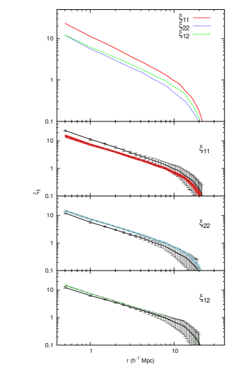
Fig. 2 shows the three corresponding partial two-point correlation functions, estimated according to Eq. (2). All three show clearly the high degree of clustering within the pattern of galaxies. It is obvious that the correlation function for the type ‘1’ passive galaxies is steeper than for the type ‘2’ active galaxies as well as for the (1,2) pairs. This result corroborates the spectral segregation detected by Madgwick et al. (2003) for the 2dFGRS.

Figure 2: The partial two-point correlation functions, $\xi_{ij}(r)$, estimated for population ‘1’ (early-type) and population ‘2’ (late-type) galaxies in our sample. The top panel shows the three functions together. The three lower panels show each of them separately (solid lines with error bars estimated using the jackknife method), together with a shaded band showing the minimum and maximum values for the 200 realizations of the random relabelling simulation. The dot-dashed lines correspond to $\xi(r)$ for the full sample, which is the expected value of all $\xi_{ij}(r)$ in the absence of segregation.

4.2 The normalized mark correlation function

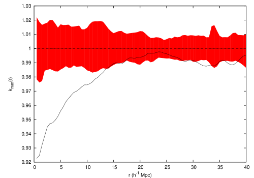
The $k_{mm}(r)$ for our sample, estimated according to Eq. (5), is shown in Fig. 3. The curve for $k_{mm}(r)$ shows a weak negative correlation or spatial inhibition: $k_{mm}(r)<1$. The range of correlation is about 20 $h^{-1}$ Mpc, where $k_{mm}(r)$ gets values close to 1. It is interesting to compare this result with the $k_{mm}(r)$-function shown in Beisbart & Kerscher (2000) using the galaxy absolute luminosity $L$ as the mark. They obtain an increasing behaviour of $k_{mm}(r)$ at small scales with $k_{mm}(r)>1$ for $r<12\,h^{-1}$ Mpc, showing that bright galaxies are stronger correlated than faint ones. In our case, the tendency of the values of $k_{mm}(r)$ to be smaller than 1 at short scales indicates that the price galaxies have to pay for being close together is to have reduced values of the marks, i.e., being more passive.

Figure 3: Normalized mark correlation function, $k_{mm}(r)$, for our sample (solid line). The shaded band shows the minimum and maximum values for the 200 realizations of the random relabelling simulation, while the dot-dashed line correspond to the value for the case with no segregation, $k_{mm}(r)=1$.

4.3 The mark variogram

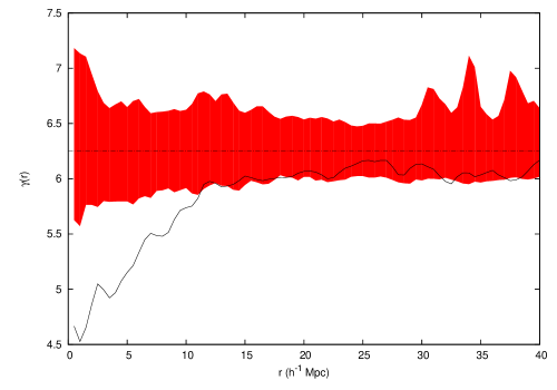
In Fig. 4, we show the mark variogram for our sample, obtained according to Eq. (7). This function is monotonously increasing. In this case the interpretation is straightforward: $\gamma(r)$ shows that, for separations $r\lesssim 10$ $h^{-1}$ Mpc, galaxy pairs tend to have similar marks, that is, similar spectral type.

This result is partially explained with the previous one shown by the $k_{mm}$ function: galaxies close together exhibit smaller values of the attached mark (spectral type).

Figure 4: Mark variogram, $\gamma(r)$, for our sample (solid line). The shaded band shows the minimum and maximum values for the 200 realizations of the random relabelling simulation, while the dot-dashed line corresponds to the value for the case with no segregation, $\gamma(r)=\sigma_{m}^{2}=6.25$.

4.4 The mark connection function

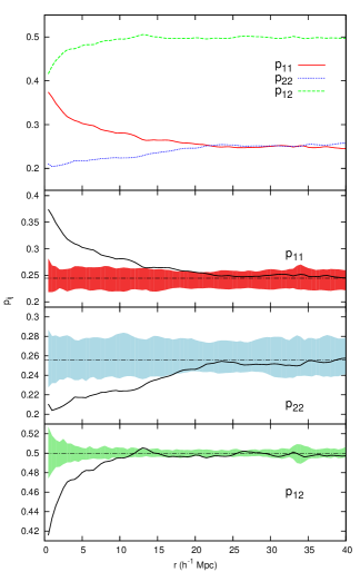
We show the $p_{ij}(r)$ obtained for the 2dFGRS galaxies, together with the results of our random relabelling simulations, in Fig. 5. The first panel shows very neatly that, for scales $r\lesssim 20$ $h^{-1}$ Mpc, the clustering of early-type galaxies is stronger than the clustering of late-type galaxies. The three bottom panels show that the deviation of the observed $p_{ij}(r)$ from the case of random labelling is significant at these scales.

Moreover, the figure shows clear differences in the spatial correlations of galaxies of the two types. In an overall clustering of all galaxies, we can outline that:

1. Galaxies of type ‘1’ (passive or early-type) are strongly clustered up to distances of 20 $h^{-1}$ Mpc.

2. The conditional probability to find two galaxies of type ‘2’ (active or late-type) at two positions separated by a distance $r$ (under the condition that at these locations are galaxies) is smaller than the same probability for random labelling of the marks for scales $r\lesssim 20$ $h^{-1}$ Mpc.

3. Galaxy pairs having one member of type ‘1’ and the other member of type ‘2’ are less frequent than for random labelling up to distances of 10 $h^{-1}$ Mpc.

In summary, all galaxies form a highly clustered pattern. In this pattern, the passive galaxies tend to be close to other passive galaxies, while positioning of active galaxies is less affected by other active galaxies. However, they tend to avoid positions close to passive galaxies.

This shows clearly the power of the mark connection function as an analytical tool in comparison to the partial pair correlation function. While, for the untrained eye, the curves in Fig. 2 are quite similar and show little structure, the curves in Fig. 5 give valuable information about the inner structure of the mark distribution. Obviously, the idea to consider characteristics of the nature of conditional probabilities helps to divulge structural details which would be otherwise overlooked.

The problem are the mutual positions, given the positions of all galaxies without mark information. Since the three partial two-point correlation functions, shown in Fig. 2, are different for a large range of scales, the marking with marks 1 and 2 can not be an independent marking, where every galaxy obtains its mark randomly, independent of the other galaxies. In contrast, there must exist a spatial correlation between the marks. As it has been shown in Fig. 5, the mark connection function is the appropriate tool to measure this correlation.

Figure 5: Mark connection functions, $p_{ij}(r)$ obtained for ‘early-type’ (population ‘1’) and ‘late-type’ (population ‘2’) galaxies in our sample. The top panel shows the three functions together. The three bottom panels show $p_{11}(r)$, $p_{22}(r)$, and $p_{12}(r)$ separately (solid lines), together with the shaded band showing the minimum and maximum values for the 200 realizations of the random relabelling simulation. The dot-dashed lines correspond to the expected values for the random labels case, according to Eq. 8.

5 Conclusions

We have used a volume-limited galaxy sample from the 2dFGRS to test different statistical measures used to disentangle mark segregation in the distribution of the galaxies. The mark attached to each galaxy of the sample was its spectral type $\eta$. For some of the statistics, the value of the mark enters directly into the functions used for measuring segregation: the normalized mark correlation function $k_{mm}(r)$ and the mark variogram $\gamma(r)$. For other functions, as the partial correlation functions or the mark connection function, the sample has been split into two populations corresponding to passive or early-type galaxies with $\eta\leq-1.4$ and active or late-type galaxies with $\eta>-1.4$. We summarise our results as follows:

1. The partial correlation functions, including the cross-correlation function, inform us about the degree of clustering of each population separately. It shows that passive galaxies exhibit stronger clustering at small separation. Nevertheless, there is no information about the spatial correlation between the marks.

2. The normalized mark correlation function shows that having smaller values of the marks, i.e., smaller values of spectral type (being more passive), is a clear condition for galaxies being close to each other in the overall clustering pattern.

3. The mark variogram, in addition, shows that at small separations galaxy pairs tend to have similar marks.

4. The mark connection function has been introduced here for the first time in the analysis of the marked galaxy distribution. The function $p_{ij}(r)$ measures the conditional probability to find at two positions, separated by a distance $r$, a galaxy of type ‘i’ and a galaxy of type ‘j’ under the condition that at these positions there are indeed galaxies. This function yields information different from that of the partial correlation functions $\xi_{ij}(r)$. This more sophisticated measure, having a nature of conditional quantities, is an efficient statistical tool to characterize the spatial correlation between the marks, filtering out the relative frequencies of the mark pairs $(i,j)$ at distance $r$.

   Applied on the 2dFGRS volume-limited sample, the mark connection function clearly shows that passive galaxies are clustered up to distances of 20 $h^{-1}$ Mpc, while active galaxies exhibit weak spatial anticorrelation of the mark up to distances of 20 $h^{-1}$ Mpc. Mixed pairs are less frequent up to distances of 10 $h^{-1}$ Mpc.