Information Asymmetries in Pay-Per-Bid Auctions
How Swoopo Makes Bank

Abstract

Innovative auction methods can be exploited to increase profits, with Shubik’s famous “dollar auction” [12] perhaps being the most widely known example. Recently, some mainstream e-commerce web sites have apparently achieved the same end on a much broader scale, by using “pay-per-bid” auctions to sell items, from video games to bars of gold. In these auctions, bidders incur a cost for placing each bid in addition to (or sometimes in lieu of) the winner’s final purchase cost. Thus even when a winner’s purchase cost is a small fraction of the item’s intrinsic value, the auctioneer can still profit handsomely from the bid fees. Our work provides novel analyses for these auctions, based on both modeling and datasets derived from auctions at Swoopo.com, the leading pay-per-bid auction site. While previous modeling work predicts profit-free equilibria, we analyze the impact of information asymmetry broadly, as well as Swoopo features such as bidpacks and the Swoop It Now option specifically, to quantify the effects of imperfect information in these auctions. We find that even small asymmetries across players (cheaper bids, better estimates of other players’ intent, different valuations of items, committed players willing to play “chicken”) can increase the auction duration well beyond that predicted by previous work and thus skew the auctioneer’s profit disproportionately. Finally, we discuss our findings in the context of a dataset of thousands of live auctions we observed on Swoopo, which enables us also to examine behavioral factors, such as the power of aggressive bidding. Ultimately, our findings show that even with fully rational players, if players overlook or are unaware any of these factors, the result is outsized profits for pay-per-bid auctioneers.

1 Introduction

One of the more interesting commercial web sites to appear recently from the standpoint of computational economics is Swoopo. Swoopo runs an auction website, using a nontraditional “pay-per-bid” auction format. Although we provide a more formal description later, the basic framework is easy to describe. As with standard eBay auctions, pay-per-bid auctions for items begin at a reserve price (generally 0), and have an associated countdown clock. When a player places a bid, the current auction price is incremented by a fixed amount, and some additional time is added to the clock. When the clock expires, the last bidder must purchase the item at the final auction price. The pay-per-bid enhancement is that each time a player increments the price and becomes the current leader of the auction, they must pay a bid fee. At Swoopo.com, the price increment typically ranges from 1 cent to 24 cents, and placing a bid typically costs 60 cents. An important variation is a fixed-price auction, where the winner obtains the right to buy the item at a fixed price $p$. When $p=0$, such an auction is referred to as a 100% off auction; in this case Swoopo derives all of its revenue from the bids.

While there are other web sites using similar auctions, Swoopo has become the leader in this area, and recently has inspired multiple papers that attempt to analyze the characteristics of the Swoopo auction [2, 4, 9]. These models share the same basic framework, based on assuming players decide whether or not to bid in a risk-neutral fashion, which we explain in detail in Section 2. Some of these papers then go further, and attempt to justify their model by analyzing data from monitoring Swoopo auctions.

One of the most interesting things about the nearly identical analyses undertaken thus far is that the simple versions of the model predict negligible profits for Swoopo, in that the expected revenue matches the value of the item sold. This fails to match the results from datasets studied in these papers, other anecdotal evidence [14, 15], as well as hard evidence we compiled from a dataset comprising over one hundred thousand auction outcomes that we collected, which show Swoopo making dramatic profits (see Figure 1). Some suggestions in previous work have been made to account for this, including the relaxation of the assumption that players are risk-neutral [9], or the addition of a regret cost to model the impact of sunk costs [2].

In this paper, we take the previous analysis as a starting point, but we focus on whether there are intrinsic aspects of the pay-per-bid auction framework that can derive profit from even rational, risk-neutral players who correctly model sunk costs. Specifically, previous work has modeled the game as inherently symmetric, with all players adopting identical randomized strategies. However, there are natural asymmetries that can arise in the Swoopo auction, particularly asymmetries in information. A rational player’s strategy revolves around his assessment of the probability of winning the auction outright by bidding, based on the current bid, the number of bidders, the bid fee, and the value of the item. Let us focus on one of these parameters, the number of players $n$. Although previous models assume that $n$ is known to all players in advance, in practice, there is no way to know exactly how many players are actively participating or monitoring the auction at any time. In Section 3, we show that even small asymmetries in beliefs about the number of active players can lead to dramatic changes in overall auction revenue, and these changes can grow sharply as the estimates vary from the true number of players. We also quantify a similar effect due to uncertain beliefs, as opposed to asymmetry across beliefs.

Figure 1: Empirical estimate of profit margins for 114,628 Swoopo ascending-price auctions. The overall profit margin is computed by summing the profit across all auctions and dividing it by the total cost.

As a related example, previous analyses assume that all players both pay the same fee to place a bid in an auction and ascribe an identical value to an item. The latter is clearly not the case, and we discuss the implications in Section 6. Less obviously, not all bidders on Swoopo are paying the same price per bid, since one item available for auction at Swoopo is a bidpack, which is effectively an option to make a fixed number of bids in future auctions for free (“freebids”). Players that win bidpacks at a discount on face value therefore have the power to make bids at a cheaper price than other players. As many players may not factor in this effect (and are unlikely in any case to be able to accurately estimate either the number of players using freebids, or the nominal bid fee those players pay), this again creates an information gap that tends to lead to increased profits for Swoopo. In this case, players using less expensive bids have a decided advantage, as we show in Section 5. Pushing this to the extreme, we have the case of shill bidders, who bid on behalf of the auctioneer, and can be modeled as bidders who incur no cost to bid (but also never claim an item). While we do not suggest shill bidders are present in online pay-per-bid auctions, our analysis in Section 7.2 nevertheless shows that they would have a striking impact on profitability.

Previous analyses also assume that no players have any available side information that they can exploit. However, two ways in which this side information may be present are when coalitions of bidders form, a case we address in Section 7.1, and the setting in which a Swoopo bidder is determined to buy the item, which we analyze in Section 8. This interesting second case is facilitated by Swoopo’s Swoop It Now feature, introduced in the US around July 2009, which enables any bidder to use all of their bid fees in an auction as a down payment for the item from Swoopo at full retail value, up until one hour after the auction concludes. Auctions containing one or more committed players who will use the Swoop It Now feature if needed ultimately reduce to games of chicken [10], an exceptionally profitable outcome for Swoopo that closely resembles auctions involving shill bidders.

Finally, our framework allows us to examine other interesting aspects of these types of auctions that are difficult to model analytically, but which can be studied via empirical observations. One question that we are particularly interested in is whether certain bidder behavior, such as aggressive bidding and bullying, is effective, as earlier work speculates [2]. In Section 8.2, we formulate a new definition of bidder aggression, and demonstrate that bidders range widely across the aggression spectrum. While aggressive bidders win more often, analysis of our dataset shows that the most aggressive bidders contribute the lion’s share of profits to Swoopo, and successful strategies are most frequently associated with below-average aggression.

We believe that modeling and analyzing these information asymmetries are interesting in their own right, although we also argue that they provide a more realistic framework and possible explanation for Swoopo profits than previous work. Indeed, our work reveals the previously hidden complexity of this auction process in the real-world setting.

We emphasize that while we provide data in an attempt to justify these additions to the model, in contrast to previous work, we eschew efforts to fit existing data to our model to parameterize and validate it. At a high level, we feel that at this stage validation attempts based on data fitting are unwarranted. Indeed, the attempt is reminiscent of similar attempts in the area of power laws in computer networks, where after many initial works attempted to justify their model of power law growth by showing it fit the data, it has been widely argued that fitting data is an improper approach for validation, as many models with very different characteristics lead to power law behaviors [6, 7, 16].

1.1 Related Work

Several recent working papers have studied pay-per-bid auctions [2, 4, 9]. While there are some differences among the papers, they all utilize the same basic framework, which is based on finding an equilibrium behavior for the players of the auction. We describe this framework in Section 2, and use it as a starting point. The key feature of this framework from our standpoint is that it treats the players as behaving symmetrically, with full information. Unsurprisingly, in such a setting the expected profit for Swoopo is theoretically zero.

Our key deviation from past work is to consider asymmetries inherent in such auctions, with a particular focus on information asymmetry. Information asymmetry broadly refers to situations where one party has better information than the others, and has become a key concept in economics, with thousands of papers on the topic. The pioneering work of Akerlof [1], Spence [13], and Stiglitz [11], for which the authors received a Nobel Prize in 2001, established the area. Typical examples of information asymmetry include insider trading, used-car sales, and insurance. Interestingly, the study of information asymmetry in auctions appears significantly less studied. We believe that our analysis of Swoopo auctions provides a simple, natural example of the potential effects of information asymmetry (as well as other asymmetries) in an auction setting, and as such may be valuable beyond the analysis itself. Indeed, our first example shows how information asymmetry about a basic parameter of an auction – the number of participants – can significantly affect its profitability.

1.2 Datasets

Where appropriate, we motivate our work or provide evidence for our results via data from Swoopo auctions. We have collected two datasets. One dataset is based on information published directly by Swoopo, which contains limited information about an auction. Information provided includes basic features such as the product description, the retail price, the final auction price, the bid fee, the price increment, and so on. This dataset covers over 121,419 auctions. We refer to this as the Outcomes dataset.

Our second dataset is based on traces of live auctions that we have ourselves recorded using our own recording infrastructure. Our traces include the same information from the Swoopo auctions as well as detailed bidding information for each auction, specifically the time and the player associated with each bid. This dataset spans 7,353 auctions and 2,541,332 bids. We refer to this as the Trace dataset. Our methodology to collect bidding information entailed continuous monitoring of Swoopo auctions. We probe Swoopo according to a varying probing interval that is described in detail in Appendix B; in particular, when the auction clock is at less than 2 minutes, we probe at least once a second. Swoopo responds with a list of up to ten tuples of the form $(username,bidnumber)$ indicating the players that placed a bid since our previous probe and the order in which they did so. Often this list would include more than one tuple. In these cases we ascribe the same timestamp to all of these bids; given the high probing frequency, this is a reasonable approximation. A more significant limitation from our methodology arises when more then ten players bid between successive probes. In these cases, Swoopo responded with just the ten latest bids. In particular this happened when more than ten players were using BidButlers, automatic bidding agents provided by the Swoopo interface, to bid at a given level. Overall, we captured every bid from 4,328 auctions. The remaining 3,025 auctions had a total of 491,360 missing bids; we did not consider these in our study.

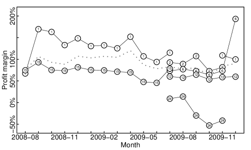
As two examples of the kind of information that can be derived from our dataset we present Figures 2 and 3, derived from the Outcomes dataset. The former presents Swoopo’s monthly profit margin for a set of what we refer to as regular auctions, grouped by price increment. Regular auctions exclude “NailBiter” auctions which do not allow the use of BidButlers, beginner auctions which are for players who have not won an auction previously, and fixed-price auctions. The latter figure displays Swoopo’s profit margin by item, for items that have been auctioned off at least 200 times in regular auctions.

Figure 2: Swoopo monthly profit margins by price increment for regular auctions from the Outcomes dataset. The dotted line represents the profit margin across all price increments.

Figure 3: Profit margin for items that have been auctioned off at least 200 times in regular auctions from the Outcomes dataset.

More details regarding the datasets can be found in Appendix B. These datasets are publicly available.

2 A Symmetric Pay-Per-Bid Model

We start with a basic model and analysis of Swoopo auctions from previous work, following the notation and framework of [9], although we note that essentially equivalent analyses have also appeared in other work [2, 4]. This serves to provide background and context for our work.

We consider an auction for an item with an objective value of $v$ to all players. There are $n$ players throughout the auction. The initial price of the item is 0. In the ascending-price version of the auction, when a player places a bid, he pays an up-front cost of $b$ dollars, and the price is incremented by $s$ dollars. The auction has an associated countdown clock; time is added to the clock when a player bids to allow other players the opportunity to bid again. When an auction terminates, the last bidder pays the current price of the item and receives the item. In a variant called a fixed-price auction, the winner buys the item for a fixed price $p$; bids still cost $b$ dollars but there is no price increment. When $p=0$, this is called a 100%-off auction. In our analysis, we simplify players’ strategies by removing the impact of timing. Instead of bidding at a given time, players choose to bid based on the current price; if multiple players choose to bid based on the current price, we generally break ties by assuming a random bidder bids first. A player that chooses not to bid at some price may bid later at a higher price.

The basic formulation for analyzing this game is that a player who makes the $q$th bid is betting $b$ than no future player will bid. Let $\mu_{j}$ be the probability that somebody makes the $j$th bid (given that $j-1$ previous bids have been made). Then the expected payoff for the player that makes the $q$th bid is $(v-sq)(1-\mu_{q+1})$; a player will only bid if this payoff is non-negative. Note that when $q>Q\equiv\lfloor\frac{v-b}{s}\rfloor$ it is clear that no rational player will bid, as the item price plus bid fee exceeds the value. For convenience in the analysis we will assume that $\frac{v-b}{s}$ is an integer, to avoid technical issues when this does not hold (see [2] for a discussion); this assumption ensures that a player that makes the $Q$th bid is indifferent to the outcome (the expected payoff is 0). In the fixed-price variant, the payoff is $(v-p)(1-\mu_{q+1})$; as long as $v>p$, bidding may occur.

The equilibrium behavior is found by determining the probability that a player should bid so that the expected payoff is zero whenever $q\leq Q$, leaving the players indifferent as to the choice of whether to bid or not to bid. (Alternative equilibria that are not germane to our analyses are discussed in [2].) Hence the indifference condition is given by

$$b=(v-sq)(1-\mu_{q+1}),$$

or

$$\mu_{q+1}=1-\frac{b}{v-sq}$$

in the ascending-price auction, and

$$\mu_{q}=1-\frac{b}{v-p}$$

at all steps in the fixed-price auction.

In what follows it is helpful to let $\beta_{q}$ be the probability that each player chooses to make the $q$th bid given that the $(q-1)$st bid has been made and that the player is not the current leader. Note that by symmetry each player bids with the same probability. Hence, for $q>1$, for ascending-price auctions we must have

$$1-\mu_{q} = (1-\beta_{q})^{n-1}$$

$$\beta_{q} = 1-(1-\mu_{q})^{1/(n-1)}$$

$$\beta_{q} = 1-\left(\frac{b}{v-s(q-1)}\right)^{1/(n-1)}.$$

Similarly, we have

$$\beta_{q}=1-\left(\frac{b}{v-p}\right)^{1/(n-1)}$$

for the fixed-price auction.

We point out that the first bid is a special case, since at that point there is no leader. To maintain consistency, we want the indifference condition to hold for the first bid; that is, players still bid such that their expected profit is zero. This requires a simple change, since at the first bid there are $n$ players who might bid instead of $n-1$, giving for the ascending-price auction

$$\beta_{q} =\begin{cases}1-\left(\frac{b}{v}\right)^{\frac{1}{n}}&\quad\textrm{for $q=1$,}\\ 1-\left(\frac{b}{v-s(q-1)}\right)^{\frac{1}{n-1}}&\quad\textrm{for $q>1$.}\end{cases}$$ (1)

Similar equations hold for the fixed-price variant:

$$\beta_{q} =\begin{cases}1-\left(\frac{b}{v-p}\right)^{\frac{1}{n}}&\quad\textrm{for $q=1$,}\\ 1-\left(\frac{b}{v-p}\right)^{\frac{1}{n-1}}&\quad\textrm{for $q>1$.}\end{cases}$$ (2)

The expected revenue for the auction can easily be calculated directly using the above quantities. However, we suggest a simple argument (that can be formalized in various ways, such as by defining an appropriate martingale) that demonstrates that Swoopo’s expected revenue is $v$ if there is at least one bid, and zero if no player bids. (A similar argument appears in [2].) First note that in auctions where there is at least one bid, an item of value $v$ is transferred to some player at the end of the auction. Also, by the indifference condition, the expected gain to the player that places any bid is zero. (Think of a bid $b$ as counterbalanced by the auctioneer putting an expected value $b$ at risk.) Therefore, by linearity of expectations, the auctioneer recoups a sum of payments equal to $v$ in expectation over the course of the auction, conditioned on there being at least one bid. The probability that no player bids is $(1-\beta_{1})^{n}$ by definition of $\beta_{1}$, and thus the expected revenue is $v(1-(1-\beta_{1})^{n})=v-b$.

To be clear, in what follows, we will always consider revenue conditioned on the auction having had at least one bid, since otherwise, the auction is essentially a non-operation for the auctioneer. We call such auctions successful.

As we noted earlier, in practice the revenue Swoopo earns per auction is much larger than $v$ on average. To help explain this, we consider the assumptions behind this model. This model assumes that the key parameters $n$, $v$, and $b$ are the same for each player and known to all. These assumptions seem hard to justify in practice: players may misestimate the total population, some may have access to cheaper bids, or they may each value the auctioned object differently. We provide some general extensions to the model for these types of variations in Section 4, but before that, we motivate our general considerations by considering the specific example where the number of players $n$ is not known.

3 Asymmetries in the Perceived Number of Bidders

3.1 Motivation

The analysis of Section 2 makes the assumption that the number of players is fixed and known throughout. This assumption has been questioned in previous work; for example, in [9], they propose a simple alternative to the standard model where participants enter and leave the auction over time. However, even in this variation, the expected number of players at each time step is known and the distribution is assumed to be Poisson, so that the end result is a small variation on the previous analysis. Here we take a different approach and consider the original model but without the assumption that every player has the same estimate of $n$, the number of players in the game.

Before diving into the analysis, we provide some motivating data from our datasets. During an auction, Swoopo provides some limited information regarding the number of players participating in the auction. Specifically, it provides a list of the bidders that have been active over the last 15 minute period. Analysis of our Trace dataset suggests this is insufficient information for determining the number of players in the auction, and in fact we suspect it can lead players to significantly underestimate the number of other players in the auction. This will prove to have dramatic impact on the analysis, and in particular on the expected revenue to Swoopo.

Figure 4: Percentage of active bidders using a 15-minute sliding window. The $x$-axis is in log scale.

Following Swoopo, we define an active bidder as someone who has bid in the last fifteen minutes. Using our Trace dataset, we observed each auction at one minute intervals, and at each time instant we computed the number of active bidders as a percentage of the total number of players who ultimately participated in the auction. The points on the curve in our plot of these values in Figure 4 can be interpreted as the percentage of all participants accounted for in Swoopo’s active bidder list as a function of time. Our plot shows that auction participation builds to a crescendo at the end of the auction, so a typical report ten minutes from the end of the auction only reports 20% of all bidders, and when that number doubles in a five minute span, it still reflects only 40% of the population. Also, note that due to the nature of the auction, there is no fixed time at which the auction ends, so even bidders making predictions based on past observations are using a certain degree of guesswork. We therefore suggest that players relying on active bidder information may well be misguided about the size of the playing field. In the following sections we analytically quantify the effect such a misestimation has on Swoopo’s expected revenues.

3.2 Analysis for Fixed-Price Auctions

For simplicity we begin with the case of fixed-price auctions. To initially frame the analysis, we further assume that the true number of players is $n$, but all players perceive the number of players as $n-k$ for some $k$ in the range $[1,n-2]$. In this case, there is still symmetry among the players, but they choose to bid based on incorrect information. Following the previous analysis, to maintain the indifference condition that the expected revenue for a player that bids at each point should be equal to their bid fee, we have $(v-p)(1-\nu_{q})=b$, where now $\nu_{q}$ is the perceived probability that someone else will place the $q$th bid. As before,

$$\nu_{q}=1-\frac{b}{v-p}.$$ (3)

Again we let $\beta_{q}$ be the probability that a player chooses to make the $q$th bid. For $q>1$ we have $(1-\nu_{q})=(1-\beta_{q})^{n-k-1}$, or $\beta_{q}=1-(1-\nu_{q})^{\frac{1}{n-k-1}}.$

Crucially, $\nu_{q}$ is not equal to $\mu_{q}$, the true probability that will make the $q$th bid. Since $(1-\mu_{q})$ equals the probability that nobody makes the $q$th bid, we have

$$1-\mu_{q} =(1-\beta_{q})^{n-1}$$

$$\mu_{q} =1-\left((1-\nu_{q})^{\frac{1}{n-k-1}}\right)^{n-1}$$

$$\mu_{q} =1-\left(\frac{b}{v-p}\right)^{\frac{n-1}{n-k-1}}.$$ (4)

Remember that the above holds for $q>1$, as for the first bid the bidding probabilities are slightly different, as explained in Section 2. To simplify the math, as an unsuccessful auction with zero bids is uninteresting, we assume the first bid has been placed. Then $\mu_{q}$ is the same at all points, so we simply call the value $\mu$. The probability that the auction lasts another $r$ bids, after the first, is given by $\mu^{r}(1-\mu)$. If we let $R$ be the revenue from a successful auction, we calculate Swoopo’s expected revenue as:

$$E[R] =b+p+b\sum_{r=0}^{\infty}r\mu^{r}(1-\mu).$$ (5)

In the simple case where $p=0$ the expected revenue is:

$$E[R]=b\left(\frac{v}{b}\right)^{\frac{n-1}{n-k-1}}.$$ (6)

Notice that when $k=0$, the expected revenue from a successful auction is indeed $v$ as had been demonstrated in previous works. Also, as $k$ appears in the exponent of the $v/b$ term, even small values of $k$ can have a significant effect on the revenue. This dramatic impact on revenue as $k$ varies is depicted for a representative auction for $100 in cash with a bid fee of $1 and 50 players in Figure 5(a). These will be our default parameters for fixed-price auctions throughout this work.

Conversely, one could consider what happens when players overestimate the population, that is to say $k<0$. As expected, the revenue for Swoopo then shrinks, incurring an overall loss as demonstrated in the left half of Figure 5(a). From our standpoint, the key feature of this graph is the asymmetry: underestimates of the player population size have significantly larger revenue effects than overestimates. If players tend to underestimate the number of players, as our empirical evidence suggests is likely, auction revenues increase dramatically.

(a) All players underestimate the population by $k$. Negative values of $k$ stand for overestimates.

(b) Half the players underestimate the population by $k$ and half overestimate it by an equal amount.

Figure 5: Expected revenue for Swoopo in a successful 100% off auction for two different population misestimation settings; $n=50$, $v=100$ and $b=1$.

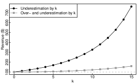
Indeed, even if the average estimated number of players is correct, when there is variation across estimates, Swoopo gains. For example, we can consider a simple case where half the players underestimate the population by $k$ and half overestimate it by the same amount. Denote by $\beta_{q,-k}$ the probability with which the former bid and similarly by $\beta_{q,+k}$ the probability with which the latter do. Then we have:

$$\beta_{q,-k} =1-(1-\nu_{q})^{\frac{1}{n-k-1}},$$ (7)

$$\beta_{q,+k} =1-(1-\nu_{q})^{\frac{1}{n+k-1}}.$$ (8)

Computing the revenue for this mixed case involves more complicated machinery which we describe in detail in Section 4. For now, we observe that even though Swoopo has far more to gain by pure underestimation of the player population, a mix of overestimation and underestimation in equal measures still yields markedly increased revenues, as depicted in Figure 5(b). (This can also be seen as a consequence of convexity of the revenue curve as the estimate of the number of players varies.)

Similar analyses can be made for different settings.

3.3 Analysis for Ascending-Price Auctions

Recall that in an ascending-price auction an auction lasts at most $Q=\lfloor\frac{v-b}{s}\rfloor$ bids subsequent to the first. Following reasoning similar to that for fixed-price auctions, we can express the expected revenue of a successful ascending-price auction where the population is underestimated by $k$ by

$$E[R]=(b+s)+\sum_{q=1}^{Q}(b+s)q(1-\mu_{q+1})\prod_{j=1}^{q}\mu_{j}$$ (9)

where $\mu_{j}=1-\left(\frac{b}{v-s(j-1)}\right)^{\frac{n-1}{n-k-1}}$. Following the same steps as [9], Equation 9 can be simplified to yield:

$$E[R] =(b+s)+\sum_{q=0}^{Q-1}\left((b+s)\prod_{j=1}^{q+1}\mu_{j}\right).$$ (10)

In an ascending-price auction, the revenue is trivially upper bounded by $(Q+1)(b+s)$, regardless of $k$. Figure 6 displays the expected revenue for Swoopo in successful auctions as the population estimation error $k$ varies. Here our auction is for $100 in cash with a bid fee of $1, 50 players, and a price increment of $0.25. Again, these will be our default parameters for ascending-price auctions throughout this work. The two dashed lines correspond to the true value of the auctioned item and the trivial upper bound on revenue of $(Q+1)(b+s)$. The plot confirms that for large enough $n$ and $k$, when $\mu_{q}\approx 1$ throughout most of the auction, this upper bound is nearly tight. Therefore, despite the asymptotic leveling off of revenues, Swoopo can still capitalize significantly from misinformed players.

Figure 6: Expected revenue as the underestimation error $k$ varies in an ascending price auction; $n=50$, $v=100$, $b=1$, and $s=0.25$.

3.4 Incorporating Uncertainty Into Population Estimates

Throughout the paper, we focus on the case where players have fixed beliefs about relevant quantities, such as the number of players participating in the game. However, it is also straightforward to extend our techniques to settings where there is underlying uncertainty within beliefs, either instead of or in addition to asymmetry across beliefs. As a concrete example, we consider the case where players are symmetric and all perceive the population size as being drawn from a distribution such that there are $i$ players with probability $p_{i}$. We do not focus on beliefs governed by distributions in the rest of the paper, because our main thematic points can be made using simpler point beliefs. Moreover, beliefs governed by distributions also raise challenging questions, such as how players determine an initial belief distribution and whether they can update their beliefs as the auction proceeds, that we do not consider in this work. However, it should intutitively be clear that uncertainty, as well as asymmmetry, can lead to situations that benefit the auctioneer. We formalize one such situation now.

Consider a fixed-price auction auction with $n$ players, where the players are symmetric and believe that the auction population size is governed by a distribution where the number of players is $i$ with probability $z_{i}$ such that $\sum_{i}iz_{i}=n$. In other words, the expectation of players’ estimates is correct, but they do not know the exact number of players. We demonstrate that players bid more frequently because of this uncertainty, leading to extra revenue for the auctioneer.

If all players think that there are $n$ players, we have the indifference condition

$$b=(v-p)(1-\nu_{q}),$$

where here $\nu_{q}$ is the the perceived probability that any other player bids. Let $\beta_{1}$ be the probability that a specific player who is not the leader bids. As $1-\nu_{q}=(1-\beta_{1})^{n-1}$, we have $\beta_{1}$ is the solution to

$$(1-\beta_{1})^{n-1}=\frac{b}{v-p}.$$

In the setting where players believe the number of players is governed by a distribution, we have the same indifference condition. However, because of the uncertainty, if we let $\beta_{2}$ be the probability that a specific player who is not the leader bids, we find

$$1-\nu_{q}=\sum_{i}z_{i}(1-\beta_{2})^{i-1},$$

since the probability that no other player bids is now given by a mixture based on the probability distribution. Hence in this setting

$$\sum_{i}z_{i}(1-\beta_{2})^{i-1}=\frac{b}{v-p}.$$

We now give a convexity argument to show that $\beta_{2}\geq\beta_{1}$; that is, there is more bidding with uncertainty. Consider

$$f(\beta)=\sum_{i}z_{i}(1-\beta)^{i-1}.$$

and

$$g(\beta)=(1-\beta)^{n-1}.$$

Note that both $f$ and $g$ are decreasing in $\beta$. Furthermore, $(1-\beta)^{x}$ is a convex function in $x$ for $\beta\in[0,1]$. Hence

$$f(\beta)=\sum_{i}z_{i}(1-\beta)^{i-1}\geq(1-\beta)^{\sum_{i}z_{i}(i-1)}=(1-\beta)^{n-1}=g(\beta).$$

Now by definition of $\beta_{2}$ and $\beta_{1}$, $f(\beta_{2})=b/(v-p)=g(\beta_{1})\leq f(\beta_{1})$. As $f$ is decreasing in $\beta$, from $f(\beta_{2})\leq f(\beta_{1})$, we have $\beta_{2}\geq\beta_{1}$, as desired.

Figure 7: Expected revenue for Swoopo when players are uncertain about the population.

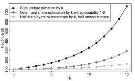
Figure 7 provides a comparison of three settings, where in all cases the number of players is $n=50$: 1) all players underestimate the number of players by $k$; 2) with probability $1/2$, all players believe that there are $n-k$ players, otherwise all believe that there are $n+k$ players; and 3) half the players believe there are $n-k$ players and half believe there are $n+k$ players. We see that for large misestimates in this setting, uncertainty provides more benefit for the auctioneer than asymmetry.

4 Extended Models for Asymmetries

We now consider a general framework in which full information is not available to all players and there are asymmetries. We describe the underlying model in Section 4.1, and in Section 4.2, we describe the analysis approach based on Markov chains that we utilize throughout the paper. We briefly discuss a full information model as an issue for future work in the conclusion.

4.1 Modeling Information Asymmetries

We now consider variations of the auction where there are asymmetries in information. For this we need to extend the symmetric model and make a crucial distinction between the true values of the game’s parameters – $v$, $b$ and $n$ – and the way players perceive them. (We motivate the misperception of each these parameters in the appropriate sections.) For simplicity, we will assume henceforth that there are two groups of players: $A$, of size $k$, and $B$, of size $n-k$. We can extend our approach to a larger number of groups naturally, but with increased complexity.

Players in group $A$ perceive the value of the item as $v^{A}$, the bid fee as $b^{A}$, and the number of participants in the game as $n^{A}$. Define $v^{B}$, $b^{B}$ and $n^{B}$ similarly. Initially, we assume that each player is asymmetry-unaware, i.e. each player assumes all players have identical parameters and thus the groups are not aware of each other. We will be also interested in cases where one group is aware of the split and therefore has an advantage over the other group. That setting will utilize the same basic structure; we develop it in later sections. In both settings, except in the special case of collusion (studied in Section 7.1), members of the groups are not aware of the identities of individuals in either group.

The parameters determine both the perceived and the true probability of the $q$th bid being placed. So, for group $A$, let $\nu_{q}^{A}$ be the perceived probability that anyone – in either group – will place the $q^{th}$ bid. In other words, $\nu_{q}^{A}$ is an estimate of $\mu_{q}$ from the perspective of players in group $A$. Also, define $\mu_{q}^{A}$ as the true probability that one or more players in group $A$ places the $q$th bid and similarly define $\nu_{q}^{B}$ and $\mu_{q}^{B}$ for group $B$. If $\mu_{q}$ is the true probability of the $q$th bid being placed then we have $1-\mu_{q}=(1-\mu_{q}^{A})(1-\mu_{q}^{B})$.

Players in group $A$ will bid according to their perceived indifference condition, which for ascending-price auctions is now $(v^{A}-s(q-1))(1-\nu_{q}^{A})=b^{A}$, and similarly for group $B$. (Similar derivations hold for fixed-price auctions.) Using the fact that $1-\nu_{q}^{A}=(1-\beta_{q}^{A})^{n-1}$ we can easily derive the individual bidding probability for group $A$ players:

$$\beta_{q}^{A}=1-\left(\frac{b^{A}}{v^{A}-s(q-1)}\right)^{\frac{1}{n^{A}-1}}.$$ (11)

The derivation for group $B$ players is identical. Using the individual bidding probabilities we can compute the probability of a bid being placed by anyone in group $A$ as

$$1-\mu_{q}^{A} =(1-\beta_{q}^{A})^{k}$$ (12)

$$\mu_{q}^{A} =1-\left(\frac{b^{A}}{v^{A}-s(q-1)}\right)^{\frac{k}{n^{A}-1}}.$$ (13)

Note that generally $\mu_{q}\neq\nu_{q}^{A}\neq\nu_{q}^{B}$.

4.2 A Markov Chain Approach for Analyzing Asymmetries

To compute various quantities of interest when we have asymmetric behaviors requires a bit of work, primarily because the probability of a bid at any given time depends in part on what group the current auction leader belongs to. In the models we have described, however, the auction itself is memoryless, in that, given the leader and the current number of bids, the history to reach the current state is unimportant to the future of the auction. Essentially all of our models have this form. Hence, we can place these auctions in the setting of Markov chains in order to efficiently calculate the distribution of auction outcomes.

Specifically, the general case for two groups of players can be captured by an absorbing, time-inhomogeneous Markov chain as shown in Figure 8. (Recall that in a time-inhomogeneous Markov chain, the transition probabilities can depend on the current time as well as the state, but not on the history of the chain.) The chain contains four states: in state $A$ a member of the first group is leading the auction, while in state $W_{A}$ the auction has been won by a member of the first group. We define states $B$ and $W_{B}$ similarly. Observe that $W_{A}$ and $W_{B}$ are absorbing states. Also observe we overload the notation $A$ and $B$ to refer both to the sets of players and a state of the Markov chain; this should not cause confusion as the meaning will be clear by context. Finally, note that there is no state corresponding to the initial setting prior to the first bid. While we could have a special initial state, we instead choose the starting state probabilistically from $A$ or $B$ according to the appropriate probabilities for the first bid, recalling that we assume our auction is successful.

Figure 8: A state-machine for an asymmetric game with two groups of players.

We use $p_{AB}(q)$ to denote the transition probability of going from state $A$ to state $B$ after the $q$th bid, and similarly we can define $p_{BA}(q)$, $p_{AA}(q)$, and so on. For example, $p_{AB}(1)$ is the transition probability from state $A$ to state $B$ when one bid has already been placed. When considering fixed-price auctions, the bidding probabilities, and hence the state transition probabilities, are invariant from bid to bid. In this special case the Markov chain becomes time-homogeneous, and given the distribution on the initial state we can derive analytical expressions for the probability of terminating in state $A$ or $B$. A good description of this approach can be found in many standard texts; we provide a summary based on [3] in Appendix A.

For ascending-price auctions, which are time-inhomogeneous, we resort to numerical methods employing simple recurrence relations. This can also be useful to obtain more specific information in the case of fixed-price auctions (or as an alternative approach for calculating various quantities). For example, let $P_{A}(q)$ be the probability of being in state $A$ after $q$ bids; here $P_{W_{A}}(q)$ represents the probability that a player from $A$ has won the auction at some point up to bid $q$, so that $P_{W_{A}}(q)+P_{W_{B}}(q)$ becomes 1 for an ascending-price auction when $q$ is sufficiently large and converges to 1 for a fixed-price auction in the limit as $q$ goes to infinity. Then we have

$$P_{A}(q+1)=P_{A}(q)p_{AA}(q)+P_{B}(q)p_{BA}(q),$$ (14)

and other similar recurrences, including

$$P_{W_{A}}(q+1)=P_{A}(q)p_{AW_{A}}(q)+P_{W_{A}}(q).$$ (15)

Given these various equations, it is easy to compute quantities such as the expected revenue. For example, in an ascending-price auction, assuming all players have a bid fee of $b$, every time $A$ is in the lead, he has paid a bid of $b$ for this, and the price has gone up by $s$. Letting $R$ be the revenue, we easily find

$$E[R]=(b+s)\left(1+\sum_{i=1}^{Q}P_{A}(i)+\sum_{i=1}^{Q}P_{B}(i)\right).$$ (16)

Notice that the simple nature of the Markov chain framework allows us to derive all the important quantities, such as the expected revenue for Swoopo, directly from the appropriate transition probabilities. Hence, in the rest of the paper, we focus on finding these probabilities. Where suitable, we explicitly derive corresponding quantities, but in other cases we implicitly use this Markov chain characterization and leave the details to the reader.

5 Asymmetries in Bid Fees

5.1 Motivation

(a) Winners’ total cost of bidpacks as a percentage of retail price (Outcomes dataset).

(b) Winners’ total cost of bidpacks as a percentage of retail price when accounting also for lost auctions (Trace dataset).

Figure 9: Measuring the acquisition cost of bidpacks

We now consider asymmetries that arise when players have different bid fees. While it seems clear that in pay-per-bid auctions players may fail to properly estimate the population of bidders, it is less clear why the cost per bid may vary among players, so we now motivate this direction.

Among other items offered on auction at Swoopo are bidpacks. A bidpack, as its name suggests, is a set of prepaid bids. As of this writing they come in five sizes: 40, 75, 150, 400, and 1000 bids. Their corresponding retail values are $24, $45, $90, $240 and $600, but if won in an auction they can potentially be had for a substantial discount. Players who win bidpack auctions and participate in later auctions can effectively enjoy lower bidding fees compared to other participants, generally without the other participants’ knowledge.

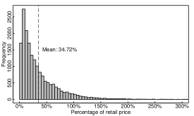
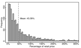
To provide evidence that bidpacks can lead to varying bid fees, we look to our data. Based on our Outcomes dataset, we derive the average cost of a bidpack as a percentage of the nominal retail cost for winners of bidpack auctions in Figure 9(a); this includes the winners’ bid costs and the price they paid. As can be seen, bids can be had at a substantial discount, with the winner’s total cost at just over $1/3$ of the retail cost on average. With the Outcomes dataset, however, we can only determine the cost of bids made by the auction winners; this clearly underestimates the costs to players who may also lose auctions for bidpacks, raising their average cost per bid. To attempt to account for this, we similarly examine our Trace dataset, and compute the average cost for any winner of a bidpack auction, including the cost for bidpack auctions where the player has lost. These results appear in Figure 9(b). Naturally, this leads to a smaller estimated average discount, although the discount is still over $1/2$ of the retail cost. While this may still be an underestimate of bidpack costs (as we cannot take into account auctions we have not captured, and our results are biased towards winners) it strongly suggests that winners of bidpack auctions enjoy a substantial discount in bid fees when applying those bids to other auctions.

Cheaper bids are also available through seasonal promotions that Swoopo conducts. For example, Swoopo has had promotions offering more bids for the same price. A screenshot showing such a promotion is given in Figure 10. A further cause for variation in bid fees relates to the remarkable fact that Swoopo auctions take place with bidders bidding in different currencies. An example of this is shown in Section 6.

Figure 10: A recent seasonal bidpack promotion.

Between bidpack auctions, seasonal promotions, and currency differences, the possibility that players are paying varying bid fees becomes reality. In the following we analyze and quantify the impact this has on Swoopo auctions.

5.2 Fixed-Price Auctions

We first consider the simpler case of fixed-price auctions with price $p$. We assume that the $n$ bidders are divided in two groups $A$ and $B$, of size $k$ and $n-k$ respectively. We will assume that $k\geq 2$; the case where $k=1$ can be handled similarly but the case structure of the analysis is slightly different. Group $A$ incurs a bid fee of $b^{A}$ while group $B$ incurs a bid fee of $b^{B}$ with $b^{A}<b^{B}$. In context, we may presume that group $A$ is the set of bidders who are bidding at a discount whereas group $B$ is the set of players who are charged regular bid fees. In what follows we also assume $A$ players are aware of the two groups while $B$ players perceive everyone as belonging to the same group as themselves. This creates an information asymmetry. We believe this choice of model is natural; we suspect many (less sophisticated) players may not recognize that others are obtaining cheaper bids. It also provides an example of how our Markov chain approach of Section 4.2 applies to such a setting.

Intuitively, players in $A$, having access to lowered bid fees, would outlast players in group $B$ in expectation. Much less obviously, it also turns out that the expected length of the auction has no dependence on the bid fee of the $B$ players – the auction length is solely determined by the bid fees incurred by the $A$ players.

Let $\mu_{q}^{A}$ be the collective probability that some player in group $A$ makes the $q$th bid, and similarly define $\mu_{q}^{B}$. Then the probability that no player makes the $q$th bid is:

$$(1-\mu_{q})=(1-\mu_{q}^{A})(1-\mu_{q}^{B})$$ (17)

where $\mu_{q}$ is defined to be the true collective probability that anyone, in either group, bids.

Next, consider the game from the point of view of $B$ players. Remember that, according to them, everyone belongs to a single group incurring the same bid fee. Define $\nu_{q}^{B}$ as the perceived probability that anyone, in either group, makes the $q$th bid according to the information available to $B$ players. From the indifference condition for $B$ players we have:

$$(v-p)(1-\nu_{q}^{B}) =b^{B}$$

$$\nu_{q}^{B} =1-\frac{b^{B}}{v-p}.$$ (18)

We derive the true probability $\beta_{q}^{B}$ that a $B$ player bids as:

$$(1-\nu_{q}^{B}) =(1-\beta_{q}^{B})^{n-1}$$

$$\beta_{q}^{B} =1-(1-\nu_{q}^{B})^{\frac{1}{n-1}}$$

$$\beta_{q}^{B} =1-\left(\frac{b^{B}}{v-p}\right)^{\frac{1}{n-1}}.$$ (19)

We can then write the probability of group $B$ bidding as:

$$1-\mu_{q}^{B}=\begin{cases}(1-\beta_{q}^{B})^{n-k}&\quad\textrm{if group $A$ is leading,}\\ (1-\beta_{q}^{B})^{n-k-1}&\quad\textrm{if group $B$ is leading},\end{cases}$$

which after manipulation becomes:

$$\mu_{q}^{B}=\begin{cases}1-\left(\frac{b^{B}}{v-p}\right)^{\frac{n-k}{n-1}}&\quad\textrm{if group $A$ is leading,}\\ 1-\left(\frac{b^{B}}{v-p}\right)^{\frac{n-k-1}{n-1}}&\quad\textrm{if group $B$ is leading.}\\ \end{cases}$$ (20)

Remember that $\mu_{q}^{B}$ is the true collective probability with which group $B$ players bid. Furthermore, notice that players in group $A$ are aware of this probability.

(a) Revenue as the price of cheap bids varies.

(b) Relative likelihood of a specific player in group $A$ winning the auction when compared with a specific player in group $B$.

Figure 11: A fixed-priced auction with $k$ players provisioned with cheap bids; $n=50$, $v=100$ and $b^{B}=1$.

Assuming the leader before the $q$th bid was from group $B$ and using the indifference condition for group $A$ we can derive an expression for $\mu_{q}^{A}$:

$$(v-p)(1-\mu_{q}^{A})(1-\mu_{q}^{B}) =b^{A}$$ (21)

$$\mu_{q}^{A} =1-\frac{b^{A}}{(v-p)(1-\mu_{q}^{B})}$$ (22)

$$\mu_{q}^{A} =1-\frac{b^{A}}{v-p}\left(\frac{v-p}{b^{B}}\right)^{\frac{n-k-1}{n-1}}$$ (23)

$$\mu_{q}^{A} =1-\frac{b^{A}}{b^{B}}\left(\frac{b^{B}}{v-p}\right)^{\frac{k}{n-1}}.$$ (24)

The derivation for group $A$ leading is similar, leading to:

$$\mu_{q}^{A}=\begin{cases}1-\frac{b^{A}}{b^{B}}\left(\frac{b^{B}}{v-p}\right)^{\frac{k-1}{n-1}}&\quad\textrm{if group $A$ is leading,}\\ 1-\frac{b^{A}}{b^{B}}\left(\frac{b^{B}}{v-p}\right)^{\frac{k}{n-1}}&\quad\textrm{if group $B$ is leading.}\\ \end{cases}$$ (25)

Next, using Equation 17 we can derive an expression for $\mu_{q}$, the true probability that a $q$th bid is placed:

$$\mu_{q}=1-\frac{b^{A}}{v-p},$$ (26)

which holds irrespectively of who is the current leader. It seems counterintuitive that neither the number of $B$ players nor their bid fee play any role in determining the probability $\mu_{q}$. However, this is similar to the original setting where all players pay the same bid fee, and $\mu_{q}$ was independent of $n$.

We can also write an expression for $\beta_{q}^{A}$:

$$\beta_{q}^{A}=\begin{cases}1-\left(\frac{b^{A}}{b^{B}}\right)^{\frac{1}{k-1}}\left(\frac{b^{B}}{v-p}\right)^{\frac{1}{n-1}}&\quad\textrm{if group $A$ is leading,}\\ 1-\left(\frac{b^{A}}{b^{B}}\right)^{\frac{1}{k}}\left(\frac{b^{B}}{v-p}\right)^{\frac{1}{n-1}}&\quad\textrm{if group $B$ is leading.}\\ \end{cases}$$ (27)

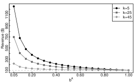
Having computed the individual bid probabilities for each player we can compute Swoopo’s expected revenue in successful auctions using the framework we developed in Section 4.2. Consider our usual fixed-price auction with $n=50$, $b=1$ and $p=0$. Some bidders have access to a discounted bid fee $b^{A}$, while the rest pay the regular rate of $1 per bid. Figure 11(a) displays Swoopo’s excepted revenue as the fee $b^{A}$ charged to group $A$ bidders for bidding varies.

The expected revenue per successful Swoopo auction actually increases, superlinearly, in the gap between bid fees. This is somewhat surprising, given that the amount of revenue from each bid from group $A$ is decreasing. We provide a high-level explanation of what appears to be happening. Group $B$ bidders not only pay full price for their bids, but are also participating in an auction that tends to last substantially longer than they expect. Furthermore, they bid with higher probability than they would if they had complete information. Consequently Swoopo’s revenues explode. Of course our analysis hinges on the assumption that group $B$ bidders never realize that they have been dealt a losing hand; recall for fixed-price auctions the underlying bidding behavior is memoryless. But, during an actual auction, Swoopo does not reveal whether a player makes a discounted bid, making it hard for players to assess how level the playing field is, and thus also making our model plausible. (We leave extensions to a setting where players change their beliefs about other auction players as the auction proceeds, and change their strategy accordingly, as future work.)

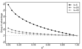
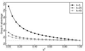
Also of interest is the advantage gained by a specific player having access to cheap bids. Using the same example as above, Figure 11(b) displays the relative likelihood of a specific $A$ player winning the auction compared to a specific $B$ player winning the auction as a function of the discounted bid fee. Observe that there is a clear synergy here: provisioning of cheaper bids helps the players who receive them and the auctioneer alike.

5.3 A Single Player with Access to Cheap Bids $(k=1)$

The analysis above depends on the size of the $A$ group of bidders being larger than one. If $k=1$, then Equations 20 and 25 do not hold any more. For completeness we provide the details for this case. (The uninterested reader may skip ahead.) In this case we have:

$$\mu_{q}^{B}=\begin{cases}1-\left(\frac{b^{B}}{v-p}\right)&\quad\textrm{if group $A$ is leading,}\\ 1-\left(\frac{b^{B}}{v-p}\right)^{\frac{n-2}{n-1}}&\quad\textrm{if group $B$ is leading,}\\ \end{cases}$$ (28)

and

$$\mu_{q}^{A}=\begin{cases}0&\quad\textrm{if group $A$ is leading,}\\ 1-\frac{b^{A}}{b^{B}}\left(\frac{b^{B}}{v-p}\right)^{\frac{1}{n-1}}&\quad\textrm{if group $B$ is leading.}\\ \end{cases}$$ (29)

Using equation 17 we can calculate the probability that a bid is placed as:

$$\mu_{q}=\begin{cases}1-\frac{b^{B}}{v-p}&\quad\textrm{if group $A$ is leading,}\\ 1-\frac{b^{A}}{v-p}&\quad\textrm{if group $B$ is leading.}\\ \end{cases}$$ (30)

Notice that, unlike the case where $k>1$, the probability of the auction ending depends on which group is currently leading the auction. This affects the duration of the auction and consequently Swoopo’s revenues. Auctions are substantially shorter when there is only one player with access to cheap bids, and similarly yield much less revenue. Figure 12(a) displays Swoopo’s revenue when $k=1$, all other parameters being unchanged. The relative advantage of a sole player with cheap bids increases dramatically, however, an effect demonstrated in Figure 12(b).

(a) Swoopo’s revenue as the price of cheap bids varies.

(b) Relative likelihood of the single player in group $A$ winning the auction when compared with a specific player in group $B$.

Figure 12: A fixed-priced auction with a single player provisioned with cheap bids; $n=50$, $v=100$ and $b^{B}=1$.

5.4 Ascending-Price Auctions

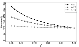
Using the methods of Section 4.1, we can also compute the expected revenue of an ascending-price auction with varying bid fees. Sample results using a price increment of $s=0.25$ are shown in Figure 13(a). Figure 13(b) displays the relative likelihood of a specific player in group $A$ winning the auction compared to a specific player in group $B$ as the price of the cheaper bid varies. The results are similar, although as one might expect, the gains to Swoopo are smaller in this setting.

(a) Swoopo’s revenue as the price of cheap bids varies.

(b) Relative likelihood of a specific player in group $A$ winning the auction when compared with a specific player in group $B$.

Figure 13: Ascending-price auctions with varying bid fees; $n=50$, $v=100$, $b^{B}=1$ and $s=0.25$.

6 Varying Object Valuations

We now consider the impact of varying the perceived value $v$ of the auctioned item among the players. There are multiple motivations for this consideration. A first motivation is that people may simply value the item differently. In particular, Swoopo provides a nominal retail value for the auction item, which is generally significantly higher than the purchase price one could easily obtain elsewhere (such as on Amazon). There may therefore be naïve players who base their valuation on the nominal retail price and more sophisticated players who know the actual retail price of an item. (This motivation is touched on briefly in [2], although our analysis is markedly different.)

Another more surprising motivation is that Swoopo runs its auctions simultaneously in multiple countries. That is, the participants in an auction often correspond to players in different countries, bidding on the local version of the Swoopo site. This necessarily introduces small inconsistencies due to the use of different currencies, so bids as well as valuations are likely to differ in some small degree. (One dollar is not a fixed whole number of euros.) But larger variations often occur because the auction corresponds to different items in different countries. This is not without justification – a certain type of TV, or monitor, or other electronic device generally would only work in its country of origin, so close substitutes have to be found for different countries. Figure 14 shows an actual example, with screenshots of an auction with the same auction ID and the same bidders at the US and German Swoopo sites, with different currencies and different items with different valuations up for auction. This strongly suggests that the case of different valuations is present in real auctions.

(a) US auction.

(b) German auction.

Figure 14: The same auction as seen from the US and German versions of the Swoopo website.

6.1 Fixed-Price Auctions

Motivated by the example of the same auction in different countries, we consider the following model. There are two groups of bidders. Group $A$ of size $k$ values the auctioned object at $\alpha v$ where $\alpha\in(0,\infty)$. Group $B$ of size $n-k$ values the same object at $v$. Furthermore, the members of each group perceive everyone as having the same valuation as themselves. The number of players, $n$, is globally known.

The indifference condition for group $A$ is $(1-\nu^{A}_{q})(\alpha v-p)=b$ where $\nu_{q}^{A}$ is again the perceived probability that anyone makes the $q$th bid according to players in group $A$. This implies that

$$\nu_{q}^{A}=1-\frac{b}{\alpha v-p}.$$ (31)

Similarly, for group $B$ we have

$$\nu_{q}^{B}=1-\frac{b}{v-p}.$$ (32)

We know that $(1-\nu^{A}_{q})=(1-\beta_{q}^{A})^{n-1}$, and similarly for group $B$. This implies that the true probabilities with which individual players in the two groups bid are

$$\beta^{A}_{q} =1-\left(\frac{b}{\alpha v-p}\right)^{\frac{1}{n-1}},$$ (33)

$$\beta^{B}_{q} =1-\left(\frac{b}{v-p}\right)^{\frac{1}{n-1}}.$$ (34)

Furthermore, the true collective probabilities of a bid being placed by either group are

$$\mu^{A}_{q} =\begin{cases}1-(\frac{b}{\alpha v-p})^{\frac{k}{n-1}}&\quad\textrm{if the current leader is in group $A$,}\\ 1-(\frac{b}{\alpha v-p})^{\frac{k-1}{n-1}}&\quad\textrm{if the current leader is in group $B$,}\\ \end{cases}$$ (35)

$$\mu^{B}_{q} =\begin{cases}1-(\frac{b}{v-p})^{\frac{n-k-1}{n-1}}&\quad\textrm{if the current leader is in group $A$,}\\ 1-(\frac{b}{v-p})^{\frac{n-k}{n-1}}&\quad\textrm{if the current leader is in group $B$,}\\ \end{cases}$$ (36)

Then the auction termination probability is $(1-\mu_{q})=(1-\mu_{q}^{A})(1-\mu_{q}^{B})$.

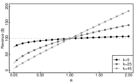
Figure 15 displays Swoopo’s revenue as the valuation parameter $\alpha$ varies from $5\%$ to $200\%$ for three different values of $k$ with $n=50$ and $b=1$. The results are natural; the more players that overvalue an item, the better for Swoopo. Unlike some of the other variations we have studied, the effects on the revenue are naturally bounded: if the maximum valuation of an item among all players is $2v$, the expected revenue in this model will not exceed $2v$. Similar results hold for ascending-price auctions.

Figure 15: Revenue for Swoopo as the valuation parameter $\alpha$ varies. Shown for three different values of $k$ and $n=50$, $v=100$, $b=1$ in a fixed-price auction.

7 Hidden Information: Collusion and Shill Bidders

The analysis for varying the number of players gives us a simple framework for analyzing two other standard situations with information asymmetry, namely where certain players have hidden information. In the first setting, we consider the case where a subset of players collude to form a bidding coalition. In the second, we consider shill bidders, or bidders in the employ of the auctioneer.

7.1 Collusion

In the setting of collusion, the natural approach is for the members of the coalition to agree to not bid against each other, so that if one of them is currently leading the auction the others bid with zero probability. The agents can either behave independently, or we can think of the coalition as a single player or agent acting on behalf of the coalition members. A benefit of colluding here is that the coalition can potentially intimidate other players from bidding, by making it appear that there are more players in the auction than there actually are, thereby reducing the probability that other players bid. We wish to quantify the advantage gained by this form of collusion in terms of the size of the coalition.

7.1.1 Fixed-Price Auctions

For our analysis, we assume that there is a group $A$ of $k$ players in a coalition, and a group $B$ of $n-k$ other players not in the coalition. To these $n-k$ players, there appear to be $n$ identical players in the auction. Again, the coalition players bid as usual, provided a coalition member is not the leader. Proceeds and expenses are shared equally between coalition members.

Non-coalition members bid according to their perceived indifference condition:

$$\nu_{q}^{B}=1-\frac{b}{v-p}.$$ (37)

This yields

$$1-\nu_{q}^{B} =(1-\beta_{q}^{B})^{n-1}$$ (38)

$$\beta_{q}^{B} =1-\left(\frac{b}{v-p}\right)^{\frac{1}{n-1}}.$$ (39)

From this we can derive the true probability of a bid by group $B$:

$$\mu_{q}^{B}=\begin{cases}1-\left(\frac{b}{v-p}\right)^{\frac{n-k}{n-1}}&\quad\textrm{if group $A$ is leading,}\\ 1-\left(\frac{b}{v-p}\right)^{\frac{n-k-1}{n-1}}&\quad\textrm{if group $B$ is leading.}\\ \end{cases}$$ (40)

We observe that players in group $B$, just as a consequence of overestimating the total population, bid less frequently than they should. This fact alone is enough for the coalition of players in group $A$ to gain an edge in winning the auction.

Next, we look at the indifference condition for a player in group $A$ when someone from group $B$ is leading the auction, as otherwise group $A$ players do not bid. Remember that both costs and proceeds are shared and that players in $A$ have full information:

$$\frac{1}{k}b =\frac{1}{k}(v-p)(1-\mu_{q})$$ (41)

$$b =(v-p)(1-\mu_{q})$$ (42)

$$b =(v-p)(1-\mu_{q}^{A})(1-\mu_{q}^{B})$$ (43)

$$\mu_{q}^{A} =1-\frac{b}{(v-p)(1-\mu_{q}^{B})}$$ (44)

$$\mu_{q}^{A} =1-\left(\frac{b}{v-p}\right)^{\frac{k}{n-1}}.$$ (45)

We can derive the individual bidding probabilities for coalition members at equilibrium. Recall as we stated earlier when group $B$ is leading the auction group $A$ players act independently. Hence

$$\beta_{q}^{A}=\begin{cases}0&\quad\textrm{if group $A$ is leading,}\\ 1-\left(\frac{b}{v-p}\right)^{\frac{1}{n-1}}&\quad\textrm{if group $B$ is leading.}\end{cases}$$ (46)

Finally, using the fact that $1-\mu_{q}=(1-\mu_{q}^{A})(1-\mu_{q}^{B})$, we can derive the following expression for the probability of a bid being placed by either group:

$$\mu_{q}=\begin{cases}1-\left(\frac{b}{v-p}\right)^{\frac{n-k}{n-1}}&\quad\textrm{if group $A$ is leading,}\\ 1-\frac{b}{v-p}&\quad\textrm{if group $B$ is leading.}\end{cases}$$ (47)

The increased chances of group $A$ winning the auction are apparent, as the auction is more likely to end when $A$ leads.

Equations 39 and 46 are nearly sufficient to determine the probabilities for our Markov chain analysis. The only remaining issue regards our choice of tie-breaking rule. In our description thus far, members of the coalition behave independently when bidding, and hence if several members of the coalition bid, we would expect each to have a chance to become the leader. We refer to this as the coalition having many bidders. We could instead imagine the coalition acting essentially as a single player controlling many identities and only selecting a single one to use at each opportunity to bid (albeit with an upwards adjusted probability of bidding, i.e., $\mu_{q}^{A}$ instead of $\beta_{q}^{A}$). In this case, the coalition would be less likely to win in case of ties.

One would expect two consequences of collusion. First, a coalition of $k$ bidders should have more than $k$ times the probability of a non-colluding bidder to win. Second, the overestimation of the actual player population should negatively impact Swoopo’s revenues. We confirm both of these consequences empirically.

(a) Revenue for Swoopo when collusion occurs.

(b) Relative likelihood of the colluding group winning the auction vs. any specific outsider.

Figure 16: Fixed-price auctions with a coalition of size $k$; $n=50$, $v=100$ and $b=1$.

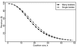
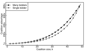
Figure 16(a) displays the revenue Swoopo can expect in the presence of a coalition of size $k$ for both tie-breaking rules. As can be seen, revenue declines significantly when large coalitions are present. Figure 16(b) displays the relative likelihood of the coalition winning the auction compared to any particular outsider. Even small groups of colluding players can gain a very large advantage in winning the auction, superlinear in the size of the coalition, offering a significant incentive to collude.

7.1.2 Ascending-Price Auctions

When considering ascending-price auctions we are faced with a time-inhomogeneous Markov chain as the bid probabilities vary in the price of the item. A closed-form solution is not as easily attainable as for time-homogeneous, fixed-price auctions. Instead we resort to the numerical evaluation methods we have described in Section 4.1. We consider our usual auction for $100 in cash with a bid fee of $1 and a price increment of 25 cents. Figures 17(a) and 17(b) respectively display the the revenue for Swoopo and the relative likelihood of a colluding bidder winning as the size of the coalition grows. The results are quite similar in this setting to the fixed-price case; a coalition can dramatically lower profits, and have a competitive advantage that grows superlinearly in their size.

(a) Revenue for Swoopo as the size $k$ of the coalition grows in an ascending price auction.

(b) Relative likelihood of the colluding group winning the auction vs. any specific outsider.

Figure 17: Ascending-price auctions with a coalition of size $k$; $n=50$, $v=100$, $b=1$ and $s=0.25$.

7.2 Shill Bidding

A further consideration is the effect of shill bidders, or bidders under the employ of the auction site who attempt to drive up revenue by bidding in order to prevent auctions from terminating early. This is not a theoretical problem; pay-per-bid auction sites other than Swoopo have been accused of using shill bidding [8]. In the working paper [9], shill bidders were considered, but it was assumed that they would behave equivalently to other players in the auction. This assumption was necessary to maintain the symmetry of the analysis, and was justified by the argument that if shill bidders behave exactly as other players, they would be more difficult to detect. We argue that sites employing shill bidding may be willing to shoulder the increased detection risk associated with increased shill bidding as long as it is accompanied by increased profit.

There are several possible ways of introducing shill bidders. Here we focus on the following natural one: we define a $(\rho,L)$-shill as one that enters the auction with probability $\rho$ and bids with probability one at each opportunity when they are not the leader until $L$ bids have been made (in total, by all players), at which stage he drops out of the auction. Such an approach provides useful tradeoffs; increasing $\rho$ or $L$ increases the probability of detection, but offers the potential for increased profit.

To analyze shill bidding we employ our usual framework. When there is no shill (with probability $1-\rho$), we assume we have a standard auction with $n$ players; with probability $\rho$ the shill enters and the auction has $n+1$ players. To analyze auctions with a shill, we separate the bidders into two groups: group $A$ consists of the lone shill, and group $B$ consists of the $n$ legitimate players who are not informed of the shill’s presence.

This information is sufficient to determine the transition probabilities in order to use our Markov chain analysis. Recall that shill bidders produce no revenue for the auctioneer, so the expected revenue is determined by the expected number of times a legitimate player is the leader. For convenience we adopt our usual tie-breaking rule, so the leader is picked uniformly at random from the players, including the shill, who decide to make a bid at each step. (One could imagine other rules – such as the shill is never picked in case of a tie, to maximize bid fees obtained.)

Before presenting some example data, we provide some intuition. We first consider a fixed-price auction with a shill bidder. The auction can be thought of as proceeding in two stages: in the first stage that lasts for up to $L$ bids the shill participates, and in the second stage the shill abstains. It should be clear that if the auction reaches the second stage the expected revenue is nearly $v$; the only issue is that there are only $n$ legitimate players, but they each behave as though there are $n+1$ players. For large enough $n$ the revenue remains close to $v$ in the second stage, and the auctioneer’s marginal profit from using a shill is therefore essentially equal to the bid fees from other players in the first stage of the auction. The case of ascending-price auctions is slightly more interesting due to the fact that legitimate players bid with decreasing probability as the price of the item goes up. As a consequence, it is more likely for the shill to win the item as $L$ increases, in which case the auctioneer only earns revenue from the bid fees.

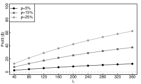
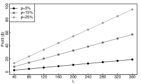
In order to see the effect of shills more clearly, rather than plot the per-auction revenue with shill bidders, we instead plot the per-auction profit. We do this for two reasons. First, since a symmetric, full-information auction results in zero expected profit for the auctioneer in our model, all profit in our plots can be attributed to the presence of the shill. Second, in this setting, there is some chance that the shill will win the auction, in which case the auctioneer’s revenue is all profit, a fact not well captured by a revenue plot. Figures 18(a) and 18(b) display the expected profit for Swoopo in the presence of a $(\rho,L)$-shill for fixed and ascending-price auctions respectively. Shill participation in ascending-price auctions has diminishing returns with $L$, which is to be expected; even though the shill is forcibly extending the expected length of the auction, as the price of the item goes up, legitimate players become less willing to participate.

(a) Fixed-price auction, $p=0$.

(b) Ascending-price auction.

Figure 18: Expected profit for Swoopo in the presence of a single-identity $(\rho,L)$-shill; $n=50$, $v=100$, $b=1$ and $s=0.25$.

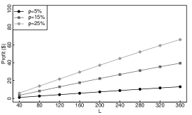
As an example of another possible shill model, we have also considered a variation where the shill player uses two distinct identities, so that he can bid with a second identity when his first identity is the leader, and vice versa. In this way, the shill can guarantee that $L$ bids will occur before dropping out of the auction, at the expense of introducing another perceived player. This approach seems riskier in terms of likelihood of detection, but leads to additional revenue, since it prevents the auction from ending early with the shill winning and thereby effectively provides more opportunities for other players to bid.

While the results for the double-identity shill plotted in Figure 19 are similar to those depicted for the single-identity shill, the profit gains due to extra bids are more substantial and the plots exhibit only minimal diminishing returns.

(a) Fixed-price auction, $p=0$.

(b) Ascending-price auction.

Figure 19: Expected profit for Swoopo in the presence of a double-identity $(\rho,L)$-shill; $n=50$, $v=100$, $b=1$ and $s=0.25$.

8 Playing Chicken and the Impact of Aggression

In this section we address a recently added feature to Swoopo’s interface, Swoop It Now, that appears to have not been analyzed previously. This feature has the potential to significantly change the dynamics of Swoopo auctions. Our suggestion is that this feature may lead to a subclass of players whose strategy makes some Swoopo auctions resemble the game of chicken [10], in contrast to the Markovian games we have modeled in previous sections. In games of chicken, it is generally understood that it can be useful for players to signal their intentions, explicitly or implicitly, to other players, in order to cause them to give up and allow the signaling player to win. A natural signaling approach in the timed auction context is to bid both frequently and quickly after another player bids. This bidding strategy has been noted previously, in the work of [2], where the author dubs this “bidding aggressively” and finds that aggressive bids have higher expected profit. Here we undertake an independent study, making several new contributions. Besides presenting how this behavior can be viewed as a signaling mechanism for a game of chicken embedded in Swoopo, we provide a novel and natural definition of aggression for pay-per-bid auctions. Then, using our trace data, we analyze auctions for signs of aggressiveness, and estimate how aggressiveness correlates with winning auctions and profitability for players. A surprising finding is that both too little and too much aggression appear to be losing strategies. We emphasize that here our analysis is based less on formal models of player behavior than in previous sections; our analysis is therefore necessarily more speculative and worthy of future study.

8.1 Swoop It Now and Chicken

Swoopo recently added the Swoop It Now option to auctions on its site, which gives each player the ability to purchase the item at a given price even if one loses the auction. That is, in many auctions, Swoopo provides a nominal retail value for the auction item, call it $r$. At the end of the auction, a player who has spent a total of $\delta$ on bids during the course of the auction can buy the item at a price of $r-\delta$; that is, the bids are transformed from otherwise unrecoverable sunk costs to a partial payment for the auction item. As argued in previous work [2, 9], the nominal retail price provided by Swoopo is generally significantly higher than the price for which one could buy the item online, and is surely well above Swoopo’s price for most items.

Unfortunately we do not currently know how often Swoop It Now is used; to our knowledge such information is neither given by Swoopo, nor derivable from any data Swoopo makes available. We suspect the feature is often overlooked, or that players are not interested, given the high nominal retail value. On the other hand, after a large losing investment in an auction, this option may become attractive to certain players.

Let us consider the behavior this additional feature introduces and its consequences in two settings: the case where only one committed player is willing to exercise this option, and the case where multiple players potentially are. Our assumption here is that $r=\alpha v$, where $v$ is a common value of the item for all players and $\alpha>1$. Our key finding is that when multiple players consider taking advantage of this option as a backstop, the game becomes a variant of chicken.

(a) Fixed-price auction.

(b) Ascending-price auction.

Figure 20: Profit for Swoopo and a committed player as $\alpha$ varies; $n=50$, $v=100$, $b=1$ and $s=0.25$.

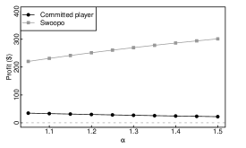
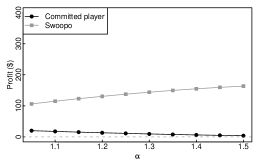
Let us first suppose that a single player has the opportunity to buy at the price $r$, including the amount they spend on bids. This player may believe the odds of winning the auction early are sufficient to keep bidding at every possible step, finding that the expected gain from winning early dominates the maximum possible loss of $(\alpha-1)v$. This player will therefore continue to bid until either winning the auction or spending enough so that it is cheaper to buy the item using Swoop It Now than to win it at the current auction price; the other $n-1$ players will play as usual. In effect, in this situation, the player is essentially equivalent to a shill bidder, except here the player keeps bidding until spending a certain amount, rather than until a certain number of bids have been made. The approach of Section 7.2 can be applied with minor variations. (In such settings, the Markov chain state space must be expanded, so this player can keep the amount spent thus far as part of the state; this is easy to accomplish.) Also, note in this case Swoopo always sells at least one copy of the item, as opposed to the setting with a shill bidder. The main outcome, naturally, is that having a player who intends to use the Swoop It Now feature increases Swoopo’s profit by prolonging the auction, assuming the presence of this player does not change other players’ strategies. Figure 20 displays the profit earned by the single committed participant as well as Swoopo. Here, as when studying shill bidders, it makes more sense to consider the profit for Swoopo. In the case where the player uses the Swoop It Now feature, if they have bid $\delta$ so far, they will have to pay an additional side payment of $r-\delta$ to complete the purchase. Also, we decrement Swoopo’s profit by an additional $v$ to account for the transfer of a second item to auction winner. The higher $\alpha$ is the longer the committed player stays in the game. As a result, profit for the committed player is decreasing in $\alpha$ while the reverse holds for Swoopo. As usual, for ascending-price auctions Swoopo’s profit is bounded - no one will bid after $Q+1$ rounds. On the other hand, if the player who is committed to the Swoop It Now purchase can signal their intention through aggressive bidding so that other players drop out of the auction, the end result is significantly less profit for Swoopo, as the auction will end early.

In the case of two (or more) players who are interested in using the Swoop It Now feature, the resulting game instead resembles the game-theoretic version of chicken. For convenience we consider a fixed-price auction with a price of $0$. Suppose that two players plan to continue to bid until either obtaining the item or spending $r$ in bids and then using the Swoop It Now feature. If both exhaust their bids, they will both lose $(\alpha-1)v$ in value. But if, instead, one of them backs off, allowing the other player to win, that player will lose only what they have bid so far – call this $\beta$ – and the other player will purchase the item at a discount – call their gain $\gamma v$, on average. Table 1 displays the chicken game in the standard payoff matrix notation.

Obviously, we have simplified things considerably in this description; there may be more than two players willing to use the Swoop It Now feature, there may be other players involved, and it may be unclear which players intend to treat the auction as a game of chicken. This is clearly a subject in need of further study. However, we do show that the Swoop It Now feature, by keeping individual losses bounded, does embed the potential for games of chicken to erupt within Swoopo auctions. As aggressive bidding is a natural way to signal intent in this setting, (and may be a sound tactic in its own right), we turn to a study of aggression, making use of our Trace dataset.

	Quit	Play Till End
Quit	$-\beta,-\beta$	$-\beta,\gamma v$
Play Till End	$\gamma v,-\beta$	$-\alpha v,-\alpha v$

Table 1: Payouts for chicken strategies

8.2 Aggression

In earlier work [2], Augenblick has suggested that aggressive bidding, including bidding immediately after another player has bid and bidding frequently in the same auction, leads to higher expected value for a player. His analysis is based on individual bids rather than bidders; that is, he considers for each bid how the time since the previous bid and the number of bids by the bidder for that item correlate to the expected profit, using regression techniques.

We adopt a different approach, by looking instead at how aggressive bidding affects the profitability of a player within an auction, and by providing a single aggression metric to measure the aggressiveness of a strategy. As a bidder may vary his strategy across auctions, we define aggressiveness in the context of a given auction. We believe that considering the effects of aggressiveness at the level of player profitability offers important insights as it views the merits of an aggressive strategy holistically. (Also, it is clear that having bid many times previously will affect the expected profit of a single bid, simply because having bid many times means the auction has gone on longer, which affects the current probability the auction terminates.)

We define an aggressive strategy as one which consists of placing many bids in rapid succession to preceding bids. Specifically, let the response time for a bid be the number of seconds since the preceding bid. Aggression should be inversely proportional to response time and proportional to the number of bids a bidder places within an auction. Hence we define the aggression of a bidder in a given auction as:

$${\mbox{Aggression}}=\frac{{\mbox{Number of bids}}}{{\mbox{Average response time (seconds/bid)}}}.$$ (48)

(a) Empirical CCDF of aggression.

(b) Cumulative profit vs. aggression rank.

Figure 21: Characterizing he profitability of aggressive strategies.

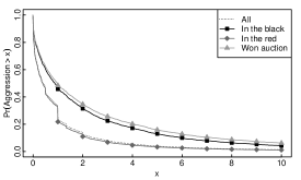
To investigate whether aggressive bidding is a successful strategy we look at the traces of 3,026 complete (no missing bids) “NailBiter” auctions (Swoopo auctions which do not permit the use of automated bids by a “BidButler”) in our Trace dataset. Figure 21(a) displays the empirical CCDF of aggression across all bidders and for three classes of strategies:

• “Won auction”: strategies that resulted in winning the auction.

• “In the black”: strategies which resulted in winning the auction profitably.

• “In the red”: strategies which resulted in losing money irrespective of whether the auction was won or lost.

(For Figure 21(a), when calculating the profit of a bidder, we assume a fixed bid cost of 60 cents, as we cannot determine the true cost. This could affect our interpretation of the results.)

Our first observation is that aggression follows a highly skewed distribution: the majority of players display little aggression, while a small number of players are highly aggressive. Also, not surprisingly, those players winning the auction were bidding much more aggressively than others. More interestingly, we see that successful players, i.e., those who not only won the auction, but did so profitably, are more aggressive than average, but less aggressive than those who win auctions. Arguably, aggression is successful in moderation.

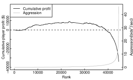
Figure 21(b) provides more insight into this latter point. For all bidder-auction pairs in our dataset, we compute the aggression and profitability of each outcome, and rank these outcomes by aggression (least aggressive first). We then plot the cumulative profit for all outcomes through a given rank with dark shading. For reference, we also plot the aggression of bidders at a given rank using light shading and the scale depicted on the right-hand side of the plot. We see that successful strategies are mostly concentrated at aggression ranks lower than average. More interestingly, a fact not evident in Figure 21(a), the highly aggressive players are responsible for most of Swoopo’s profits.

Aggressive	Number of	Auction revenue	Mean winner
bidders	auctions	(as % of retail price)	profit margin
$0$	1,699	62%	77%
$1$	493	135%	51%
$\geq 2$	834	246%	26%

Table 2: Evidence of chicken

In Table 2, we give empirical evidence that Swoopo profits are strongly and positively impacted by the presence of multiple aggressive players, defined as players with an aggression level of at least 3 bids²/sec. Strikingly, when two or more aggressive players are present, Swoopo’s per-auction revenues are in excess of 2.4 times the stated retail price of the good. At the same time, and as expected, as the number of aggressive players in an auction increases the profit margin of the auction winner decreases. The fourth column of Table 2 displays the mean of winner profit margins.

Finally, having provided empirical evidence regarding aggressive behavior, we now revisit the question of whether games of chicken are also taking place within Swoopo. To do that we turn to the Trace dataset and look at the 3,026 “NailBiter” auctions for evidence of duels: auctions culminating in long sequences of back-and-forth bidding between two opponents. We find that 9% of all auctions culminated in a duel lasting at least 10 bids, 5% lasted at least 20 bids, and 1% lasted at least 50 bids. The longest duel we observed was 201 bids long and somewhat humorously took place between users Cikcik and Thedduell. We believe this provides further evidence that at least some auctions are becoming essentially games of chicken, and reiterate our supposition that aggressive bidding is used as a signaling method in such settings.

9 Conclusions and Future Work

Swoopo provides a fascinating case study in how new, non-trivial auction mechanisms perform in real-world situations, and it also provides a focal point for developing the theory of auction mechanisms in the context of human behaviors. Here we have focused on the key issue of asymmetry, and in particular, how various manifestations of information asymmetry may be responsible in large part for the significant profits Swoopo appears to enjoy today. At the same time, we have also shown that the profitability of these auctions is potentially fragile, especially in cases where signaling by committed players willing to play a game of chicken or collusion between players can end the auction early. In these settings, information asymmetry can potentially reduce the profits enjoyed by the auctioneer.

There are clearly many interesting directions to follow from here. One area we have started to examine is asymmetric models of pay-per-bid auctions with full information. For example, players could have differing bid fees or valuations of the item, but with these fees and valuations known in advance to all players. Although a full information setting may not be as immediately practical as that considered in our work, asymmetries expose a richer set of issues than the symmetric, full information case, and have not yet been considered in any depth in previous work.

Let us consider what such a model might look like. For convenience, let us consider a fixed-price auction. Suppose that there are players $A_{1},A_{2},\ldots,A_{n}$, with player $A_{i}$ having bid fee $b^{A_{i}}$ and value $v^{A_{i}}$. Let $\beta_{A_{i}}$ be the probability that $A_{i}$ should bid when $A_{i}$ is not in the lead in equilibrium. The indifference condition for player $A_{i}$ is now given simply by:

$$b^{A_{i}}=(v^{A_{i}}-p)\left(1-\prod_{j\neq i}\beta_{A_{j}}\right),$$

or

$$\prod_{j\neq i}\beta_{A_{j}}=1-\frac{b^{A_{i}}}{(v^{A_{i}}-p)}.$$

It is helpful to substitute $\eta_{i}=\ln\beta_{A_{i}}$ and $\zeta_{i}=\ln\left(1-\frac{b^{A_{i}}}{(v^{A_{i}}-p)}\right)$. Then we can readily solve the family of simple linear equations:

$$\sum_{j\neq i}\eta_{A_{j}}=\zeta_{i}.$$

This assumes an equilibrium based on the indifference condition (and, for example, that $\beta_{A_{i}}\neq 0$). It would be interesting to consider under what conditions such equilibria exist, as well as if they are the only equilibria. In some cases, the auction might for example reduce to a game of chicken, in which case there may be multiple equilibria. For the case of ascending-price auctions, the calculations are more challenging: one can use backward induction, finding the probabilities for the $Q$th bid and then calculating downward.

It is worth noting that with varying bids, in a full information auction where all players ascribe the same value $v$ to an item and use a strategy based on the indifference condition, Swoopo’s expected revenue for successful auctions remains $v$ following the same argument as given in Section 2. This highlights the key role of information asymmetry in our result showing that varying bids can lead to large profits for Swoopo. Further comparisons with a full information model should be similarly enlightening.

Another broad topic for future work regards more extensive study of user behavior on Swoopo. While our study considers the impact of one natural tactic, aggression, in Swoopo auctions, there are many others that could also be considered. The impact of timing has generally been abstracted away, but it is probably important to user behavior, as our study of aggression suggests. More understanding of the impact of timing considerations appears important for further study. In particular, perhaps there are timing-based or other active signaling mechanisms that a strategic player could leverage to maximize expected return in these auctions. A possible direction related to signaling is the issue of learning. Can players dynamically change their beliefs about underlying auction parameters, such as the bid fee other players are charged or the intentions of other players, based on how the auction proceeds in order to improve their performance? As another example, one feature that we have not yet studied is the impact of bidders who use automatic bidding agents, such as BidButlers: how do they influence the auction, and can such bidders be detected? And finally, there remains the thorny problem of attempting to quantify the impact of how specific auction characteristics we have considered – misestimates of the number of players, varying bid fees, varying valuations of items, the ability for players to use the BidButler and the Swoop It Now features – on real-world profitability. Such an effort would likely require more detailed information regarding bids currently available only to Swoopo, and better models of user behavior.

10 Acknowledgments

Michael Mitzenmacher would like to thank Maher Said for several helpful discussions regarding Swoopo. Georgios Zervas would like to thank Azer Bestavros for helpful discussions regarding collusion.

Appendix A Computing the Steady State of a Markov Chain

Let $f(k;n,p)$ be the probability mass function of the binomial distribution where $n$ is the number of trials, $k$ is the number of successes and $p$ it the probability of success. The transition probabilities in Figure 8, presented in Section 4.2, are given by:

$$p_{AA} =\sum_{i=1}^{k-1}\sum_{j=0}^{n-k}f(i;k-1,\beta_{q}^{A})f(j;n-k,\beta_{q}^{B})\frac{i}{i+j}$$ (49)

$$p_{AB} =\sum_{i=0}^{k-1}\sum_{j=1}^{n-k}f(i;k-1,\beta_{q}^{A})f(j;k-1,\beta_{q}^{B})\frac{j}{i+j}$$ (50)

$$p_{BB} =\sum_{i=0}^{k}\sum_{j=1}^{n-k-1}f(i;k,\beta_{q}^{A})f(j;n-k-1,\beta_{q}^{B})\frac{j}{i+j}$$ (51)

$$p_{BA} =\sum_{i=1}^{k}\sum_{j=0}^{n-k-1}f(i;k,\beta_{q}^{A})f(j;n-k-1,\beta_{q}^{B})\frac{i}{i+j}$$ (52)

where $\beta_{q}^{A}$ and $\beta_{q}^{B}$ are the individual bidding probabilities of players in group $A$ and group $B$ respectively. Their exact values will depend on the specific asymmetry we are considering.

We will be interested in computing the steady state probability distribution of the Markov chain. The goal of finding closed-form solutions for time-inhomogeneous Markov chains for ascending price auctions is beyond the scope of our work; hence for these chains we resort to numerical methods, simply calculating the probability of being in each state in each stage, as described in Section 4.2. But for fixed-price auctions the analysis is far more straightforward and we present it here following the framework of [3]. First define the labeled transition matrix $P$ as:

$$P=\left(\begin{array}[]{ccccc}&\mathbf{A}&\mathbf{B}&\mathbf{W_{A}}&\mathbf{W_{B}}\\ \mathbf{A}&p_{AA}&p_{AB}&1-p_{AA}-p_{AB}&0\\ \mathbf{B}&p_{BA}&p_{BB}&0&1-p_{BB}-p_{BA}\\ \mathbf{W_{A}}&0&0&1&0\\ \mathbf{W_{B}}&0&0&0&1\\ \end{array}\right)$$ (53)

$P$ is in canonical form with the transient states coming before the absorbing ones. Let $Q$ be the submatrix of $P$ containing solely the transient states $A$ and $B$. For an absorbing Markov chain $P$ the matrix $N=(I-Q)^{-1}$ is called its fundamental matrix. The entry $n_{ij}$ of $N$ gives the expected number of times the process is in state $j$ given that it started in state $i$. Notice that $N$ exists and is equal to $I+Q^{2}+Q^{3}+\cdots$. We can express $N$ in terms of the transition probabilities:

$$N=\left(\begin{array}[]{cc}\frac{1-p_{BB}}{p_{BB}p_{AA}-p_{AA}-p_{BB}-p_{AB}p_{BA}+1}&\frac{p_{AB}}{p_{BB}p_{AA}-p_{AA}-p_{BB}-p_{AB}p_{BA}+1}\\ \frac{p_{BA}}{p_{BB}p_{AA}-p_{AA}-p_{BB}-p_{AB}p_{BA}+1}&\frac{1-p_{AA}}{p_{BB}p_{AA}-p_{AA}-p_{BB}-p_{AB}p_{BA}+1}\end{array}\right).$$ (54)

For any given starting state we can compute the time to absorption by computing the vector $t=Nc$, where $c$ is a column vector whose entries are $1$. Effectively, by adding together the elements of $N$ row-wise we are summing up the time spent in each of the transient states. In particular we have

$$t=\left(\begin{array}[]{c}\frac{-p_{AB}+p_{BB}-1}{p_{AA}(-p_{BB})+p_{AA}+p_{AB}p_{BA}+p_{BB}-1}\\ \frac{-p_{AA}+p_{BA}+1}{(p_{AA}-1)(p_{BB}-1)-p_{AB}p_{BA}}\end{array}\right).$$ (55)

Let $p_{A}$ and $p_{B}$ be the probabilities of the game starting in states $A$ and $B$ respectively and let $p_{0}$ be a vector containing them. It is worth highlighting here that $p_{A}+p_{B}<1$ as there is always the probability that nobody will place the first bid. We can compute the expected number of bids the game will last by calculating $tp_{0}$. Alternatively, as we often do, if we wish to assume that first bid always occurs $p_{0}$ has to be scaled by $1/(p_{A}+p_{B})$ so that $p_{A}+p_{B}=1$.

We will also be interested in computing the revenue of the auction. When players are charged a single bid fee the revenue can be easily obtained from expected number of bids. If the two groups of players are charged differently the revenue of is given by $p_{0}Nb$ where $b$ is a vector of bid fees.

Next, define $R$ as the upper-right, two-by-two submatrix of $P$. Let $S$ be a matrix whose $(i,j)^{th}$ element is the probability that the chain will be absorbed in state $j$ given that it started in state $i$. Then

$$S=NR=\left(\begin{array}[]{cc}\frac{\left(p_{AA}+p_{AB}-1\right)\left(p_{BB}-1\right)}{\left(p_{AA}-1\right)\left(p_{BB}-1\right)-p_{AB}p_{BA}}&\frac{p_{AB}\left(p_{BB}+p_{BA}-1\right)}{p_{AB}p_{BA}-\left(p_{AA}-1\right)\left(p_{BB}-1\right)}\\ -\frac{\left(p_{AA}+p_{AB}-1\right)p_{BA}}{\left(p_{AA}-1\right)\left(p_{BB}-1\right)-p_{AB}p_{BA}}&\frac{\left(p_{AA}-1\right)\left(p_{BB}+p_{BA}-1\right)}{\left(p_{AA}-1\right)\left(p_{BB}-1\right)-p_{AB}p_{BA}}\end{array}\right).$$ (56)

We can also compute the unconditional probabilities $w$ of the chain being absorbed in each of the sink states assuming the first bid is placed (using the scaled version of $p_{0}$):

$$w=p_{0}S=\left(\begin{array}[]{c}\frac{\left(p_{AA}+p_{AB}-1\right)\left(p_{BB}-1\right)p_{A}-p_{AB}\left(p_{BB}+p_{BA}-1\right)p_{B}}{\left(p_{AA}-1\right)\left(p_{BB}-1\right)-p_{AB}p_{BA}}\\ \frac{\left(p_{AA}-1\right)\left(p_{BB}+p_{BA}-1\right)p_{B}-\left(p_{AA}+p_{AB}-1\right)p_{BA}p_{A}}{\left(p_{AA}-1\right)\left(p_{BB}-1\right)-p_{AB}p_{BA}}\end{array}\right)^{\prime}.$$ (57)

This framework will allow us to characterize a series of asymmetries by computing the vectors $t$ and $w$, analytically where possible and computationally otherwise.

Appendix B Dataset Description

In this section we provide more information about the two datasets we collected and used throughout this paper. The dataset is publicly available at http://cs-people.bu.edu/zg/swoopo-dataset.tar.gz.

B.1 Outcomes Dataset

Our Outcomes dataset comprises 121,419 auctions conducted between September 8, 2008 and December 12, 2009. For each auction we collected the following information:

Field name	Description	Example value
auction_id	A unique numerical id for the auction.	259070
product_id	A unique product id.	10011706
item	A text string describing the product.	300-bids-voucher
desc	More information about the product.	300 Bids Voucher
retail	The stated retail value of the item, in dollars.	180
price	The price the auction reached, in dollars.	31.26
finalprice	The price charged to the winner in dollars.	31.26
bidincrement	The price increment of a bid, in cents.	6
bidfee	The cost incurred to make a bid, in cents.	60
winner	The winner’s username.	Schonmir1500
placedbids	The number of paid bids placed by the winner.	106
freebids	The number of free bids place by the winner.	0
endtime_str	The auction’s end time.	13:29 PDT 12-12-2009
flg_click_only	A binary flag indicating a “NailBiter” auction.	1
flg_beginnerauction	A binary flag indicating a beginner auction.	0
flg_fixedprice	A binary flag indicating a fixed-price auction.	0
flg_endprice	A binary flag indicating a 100%-off auction.	0

B.2 Trace Dataset

Our Trace dataset comprises 7,352 auctions conducted between October 1, 2009 and December 12, 2009. In addition to the information contained in the Outcomes dataset, our Trace dataset also contains information about the actual bids that were placed during the auction. We probed Swoopo at semi-regular time-intervals - more frequently near the end of the auction when bids are placed in rapid succession, less frequently near the beginning of the auction when bidding is sparse. Specifically, to avoid inundating Swoopo with useless requests we implemented the following back-off procedure. Our initial probing interval is set to one second. When the countdown clock had more than 10 minutes left on it, and there were no bids reported in our last request, we would increase our probing interval by half a second, up to a maximum of a minute. A new request including at least one bid would reset the probing interval to one second. When the countdown clock had at least 2 and less than 10 minutes left on it, our maximum probing interval was 10 seconds. Finally, when the countdown clock had fewer than 2 minutes left on it we probed at the rate Swoopo suggested but at least once every second (every probe response was associated with a Swoopo defined update-interval that Swoopo uses to instruct the user’s browser when to next update). Swoopo would respond with a line of the following format:

ct=15|cs=1|ra=0|cw=Schonmir1500|cp=3126|bh=521:Schonmir1500:1:3126:0:#|lui=4#1#0#0

Each line was timestamped on our end to provide the actual time of the bid(s). In plain English the above line tells us that the 521st bid of the auction was placed by user Schonmir1500. It raised the price of the item to $31.26 and it was not placed by a BidButler. Finally, when the bid was placed another 4 seconds were added to countdown clock to reset it to its current value of 15. Specifically, the fields, which are separated using vertical bars, carry the following information:

Field name	Description
ct	Current time on the countdown clock.
cs	Current state, 1 means the auction is still active, 20 that is has ended. Swoopo defines more status codes which we did not encounter.
ra	Technical use. When set to 1 forces the browser to reload the page, irrelevant to the auction.
cw	Username of current winner.
cp	Current price in cents.
bh	Bid history, #-separated tuples of the form: bidnumber:username:bidtype: price:yourbid. A bidtype of 1 indicates a player bid whereas a bidtype of 2 indicates a BidButler bid. The field yourbid is set to 1 when the observer has placed the corresponding bid.
lui	Last update index, four #-separated numbers: seconds added to clock from player bids, number of player bids, seconds added to clock by BidButler bids, number of BidButler bids.

References

- [1] G. A. Akerlof. The market for “lemons”: Quality uncertainty and the market mechanism. The Quarterly Journal of Economics, 84(3):488–500, 1970.
- [2] N. Augenblick. Consumer and Producer Behavior in the Market for Penny Auctions: A Theoretical and Empirical Analysis. Unpublished manuscript. Available at www.stanford.edu/~ned789, 2009.
- [3] C. M. Grinstead and J. L. Snell. Introduction to Probability. American Mathematical Society, 1997.
- [4] T. Hinnosaar. Penny Auctions. Unpublished manuscript at http://toomas.hinnosaar.net/, 2009.
- [5] V. Krishna and J. Morgan. An analysis of the war of attrition and the all-pay auction. Journal of Economic Theory, 72(2):343–362, 1997.
- [6] M. Mitzenmacher. A brief history of generative models for power law and lognormal distributions. Internet mathematics, 1(2):226–251, 2004.
- [7] M. Mitzenmacher. Editorial: The future of power law research. Internet Mathematics, 2(4):525–534, 2005.
- [8] http://www.pennyauctionwatch.com/tag/shills/.
- [9] B. C. Platt, J. Price, and H. Tappen. Pay-to-Bid Auctions. Unpublished manuscript. Available at http://econ.byu.edu/Faculty/Platt, 2009.
- [10] A. Rapoport and A. Chammah. The game of chicken. American Behavioral Scientist, 10, 1966.
- [11] M. Rothschild and J. Stiglitz. Equilibrium in competitive insurance markets: An essay on the economics of imperfect information. The Quarterly Journal of Economics, 90(4):629–649, 1976.
- [12] M. Shubik. The dollar auction game: a paradox in noncooperative behavior and escalation. Journal of Conflict Resolution, 15(1):109–111, March 1971.
- [13] M. Spence. Job market signaling. The Quarterly Journal of Economics, 87(3):355–374, 1973.
- [14] B. Stone. Sites ask users to spend to save. New York Times, August 17, 2009.
- [15] R. H. Thaler. Paying a price for the thrill of the hunt. New York Times, November 15, 2009.
- [16] W. Willinger, D. Alderson, and J. Doyle. Mathematics and the internet: A source of enormous confusion and great potential. Notices of the American Mathematical Society, 56(5):586–599, 2009.