Learning the Structure of Deep Sparse Graphical Models

Abstract

Deep belief networks are a powerful way to model complex probability distributions. However, learning the structure of a belief network, particularly one with hidden units, is difficult. The Indian buffet process has been used as a nonparametric Bayesian prior on the directed structure of a belief network with a single infinitely wide hidden layer. In this paper, we introduce the cascading Indian buffet process (CIBP), which provides a nonparametric prior on the structure of a layered, directed belief network that is unbounded in both depth and width, yet allows tractable inference. We use the CIBP prior with the nonlinear Gaussian belief network so each unit can additionally vary its behavior between discrete and continuous representations. We provide Markov chain Monte Carlo algorithms for inference in these belief networks and explore the structures learned on several image data sets.

journalname , and

t1http://www.cs.toronto.edu/~rpa

1 Introduction

The belief network or directed probabilistic graphical model (Pearl, 1988) is a popular and useful way to represent complex probability distributions. Methods for learning the parameters of such networks are well-established. Learning network structure, however, is more difficult, particularly when the network includes unobserved hidden units. Then, not only must the structure (edges) be determined, but the number of hidden units must also be inferred. This paper contributes a novel nonparametric Bayesian perspective on the general problem of learning graphical models with hidden variables. Nonparametric Bayesian approaches to this problem are appealing because they can avoid the difficult computations required for selecting the appropriate a posteriori dimensionality of the model. Instead, they introduce an infinite number of parameters into the model a priori and inference determines the subset of these that actually contributed to the observations. The Indian buffet process (IBP) (Griffiths and Ghahramani, 2006; Ghahramani et al., 2007) is one example of a nonparametric Bayesian prior and it has previously been used to introduce an infinite number of hidden units into a belief network with a single hidden layer (Wood et al., 2006).

This paper unites two important areas of research: nonparametric Baye-sian methods and deep belief networks. To date, work on deep belief networks has not addressed the general structure-learning problem. We therefore present a unifying framework for solving this problem using nonparametric Bayesian methods. We first propose a novel extension to the Indian buffet process — the cascading Indian buffet process (CIBP) — and use the Foster-Lyapunov criterion to prove convergence properties that make it tractable with finite computation. We then use the CIBP to generalize the single-layered, IBP-based, directed belief network to construct multi-layered networks that are both infinitely wide and infinitely deep, and discuss useful properties of such networks including expected in-degree and out-degree for individual units. Finally, we combine this framework with the powerful continuous sigmoidal belief network framework (Frey, 1997). This allows us to infer the type (i.e., discrete or continuous) of individual hidden units—an important property that is not widely discussed in previous work. To summarize, we present a flexible, nonparametric framework for directed deep belief networks that permits inference of the number of hidden units, the directed edge structure between units, the depth of the network and the most appropriate type for each unit.

2 Finite Belief Networks

We consider belief networks that are layered directed acyclic graphs with both visible and hidden units. Hidden units are random variables that appear in the joint distribution described by the belief network but are not observed. We index layers by $m$, increasing with depth up to $M$, and allow visible units (i.e., observed variables) only in layer ${m\!=\!0}$. We require that units in layer $m$ have parents only in layer ${m\!+\!1}$. Within layer $m$, we denote the number of units as $K^{(m)}$ and index the units with $k$ so that the $k$th unit in layer $m$ is denoted $u^{(m)}_{k}$. We use the notation $\boldsymbol{u}^{(m)}$ to refer to the vector of all $K^{(m)}$ units for layer $m$ together. A binary ${K^{(m-1)}\!\times\!K^{(m)}}$ matrix $\boldsymbol{Z}^{(m)}$ specifies the edges from layer $m$ to layer ${m\!-\!1}$, so that element ${Z^{(m)}_{k,k^{\prime}}\!=\!1}$ iff there is an edge from unit $u^{(m)}_{k^{\prime}}$ to unit $u^{(m-1)}_{k}$.

A unit’s activation is determined by a weighted sum of its parent units. The weights for layer $m$ are denoted by a ${K^{(m-1)}\!\times\!K^{(m)}}$ real-valued matrix $\boldsymbol{W}^{(m)}$, so that the activations for the units in layer $m$ can be written as ${\boldsymbol{y}^{(m)}\!=\!(\boldsymbol{W}^{(m+1)}\!\odot\!\boldsymbol{Z}^{(m+1)})\boldsymbol{u}^{(m+1)}\!+\!\boldsymbol{\gamma}^{(m)}}$, where $\boldsymbol{\gamma}^{(m)}$ is a $K^{(m)}$-dimen-sional vector of bias weights and the binary operator $\odot$ indicates the Hada-mard (elementwise) product.

To achieve a wide range of possible behaviors for the units, we use the nonlinear Gaussian belief network (NLGBN) (Frey, 1997; Frey and Hinton, 1999) framework. In the NLGBN, the distribution on $u^{(m)}_{k}$ arises from adding zero mean Gaussian noise with precision $\nu^{(m)}_{k}$ to the activation sum $y^{(m)}_{k}$. This noisy sum is then transformed with a sigmoid function $\sigma(\cdot)$ to arrive at the value of the unit. We modify the NLGBN slightly so that the sigmoid function is from the real line to $(-1,1)$, i.e. ${\sigma:\mathbb{R}\!\to\!(-1,1)}$, via ${\sigma(x)=2/(1+\exp\{x\})-1}$. The distribution of $u^{(m)}_{k}$ given its parents is then

$$p(u^{(m)}_{k}|y^{(m)}_{k},\nu^{(m)}_{k})=\frac{\exp\left\{\!-\frac{\nu^{(m)}_{k}}{2}\!\left[\sigma^{-1}(u^{(m)}_{k})\!-\!y^{(m)}_{k}\right]^{2}\right\}}{\sigma^{\prime}(\sigma^{-1}(u^{(m)}_{k}))\sqrt{2\pi/\nu^{(m)}_{k}}}$$

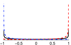
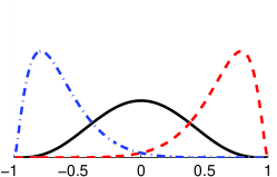
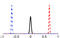
where $\sigma^{\prime}(x)\!=\!\frac{\mathrm{d}}{\mathrm{d}x}\sigma(x)$. As discussed in Frey (1997) and shown in Figure 1, different choices of $\nu^{(m)}_{k}$ yield different belief unit behaviors from effectively discrete binary units to nonlinear continuous units. In the multilayered construction we have described here, the joint distribution over the units in a NLGBN is

$$p(\{\boldsymbol{u}^{(m)}\}^{M}_{m=0}\,|\,\{\boldsymbol{Z}^{(m)},\boldsymbol{W}^{(m)}\}^{M}_{m=1},\{\boldsymbol{\gamma}^{(m)},\{\nu^{(m)}_{k}\}^{K^{(m)}}_{k=1}\}^{M}_{m=0},)=\\ \left[\prod^{K^{(M)}}_{k=1}p(u^{(M)}\,|\,\gamma^{(M)}_{k},\nu^{(M)}_{k})\right]\prod^{M-1}_{m=0}\prod^{K^{(m)}}_{k=1}p(u^{(m)}_{k}\,|\,y^{(m)}_{k},\nu^{(m)}_{k}).$$ (1)

3 Infinite Belief Networks

Conditioned on the number of layers $M$, the layer widths $K^{(m)}$ and the network structures $\boldsymbol{Z}^{(m)}$, inference in belief networks can be straightforwardly implemented using Markov chain Monte Carlo (Neal, 1992). Learning the depth, width and structure, however, presents significant computational challenges. In this section, we present a novel nonparametric prior, the cascading Indian buffet process, for multi-layered belief networks that are both infinitely wide and infinitely deep. By using an infinite prior we avoid the need for the complex dimensionality-altering proposals that would otherwise be required during inference.

(a) $\nu=\frac{1}{2}$

(b) $\nu=5$

(c) $\nu=1000$

Figure 1: Three modes of operation for the NLGBN unit. The black solid line shows the zero mean distribution (i.e. $y\!=\!0$), the red dashed line shows a pre-sigmoid mean of $+1$ and the blue dash-dot line shows a pre-sigmoid mean of $-1$. (a) Binary behavior from small precision. (b) Roughly Gaussian behavior from medium precision. (c) Deterministic behavior from large precision.

3.1 The Indian buffet process

Section 2 used the binary matrix $\boldsymbol{Z}^{(m)}$ as a convenient way to represent the edges connecting layer $m$ to layer ${m\!-\!1}$. We stated that $\boldsymbol{Z}^{(m)}$ was a finite ${K^{(m-1)}\!\times\!K^{(m)}}$ matrix. We can use the Indian buffet process (IBP) (Griffiths and Ghahramani, 2006) to allow this matrix to have an infinite number of columns. We assume the two-parameter IBP (Ghahramani et al., 2007), and use ${\boldsymbol{Z}^{(m)}\!\sim\!{\sf IBP}(\alpha,\beta)}$ to indicate that the matrix $\boldsymbol{Z}^{(m)}\!\in\!\{0,1\}^{K^{(m-1)}\times\infty}$ is drawn from an IBP with parameters $\alpha,\beta>0$. The eponymous metaphor for the IBP is a restaurant with an infinite number of dishes available. Each customer chooses a finite set of dishes to taste. The rows of the binary matrix correspond to customers and the columns correspond to dishes. If the $j$th customer tastes the $k$th dish, then ${Z_{j,k}\!=\!1}$, otherwise ${Z_{j,k}\!=\!0}$. The first customer into the restaurant samples a number of dishes that is Poisson distributed with parameter $\alpha$. After that, when the $j$th customer enters the restaurant, she selects dish $k$ with probability $\eta_{k}/(j\!+\!\beta\!-\!1)$, where $\eta_{k}$ is the number of previous customers that have tried the $k$th dish. She then chooses a number of additional dishes to taste that is Poisson distributed with parameter $\alpha\beta/(j\!+\!\beta\!-\!1)$. Even though each customer chooses dishes based on their popularity with previous customers, the rows and columns of the resulting matrix $\boldsymbol{Z}^{(m)}$ are infinitely exchangeable.

As in Wood et al. (2006), if the model of Section 2 had only a single hidden layer, i.e. $M\!=\!1$, then the IBP could be used to make that layer infinitely wide. While a belief network with an infinitely-wide hidden layer can represent any probability distribution arbitrarily closely (Le Roux and Bengio, 2008), it is not necessarily a useful prior on such distributions. Without intra-layer connections, the the hidden units are independent a priori. This “shallowness” is a strong assumption that weakens the model in practice and the explosion of recent literature on deep belief networks (see, e.g. Hinton et al. (2006); Hinton and Salakhutdinov (2006)) speaks to the empirical success of belief networks with more hidden structure.

3.2 The cascading Indian buffet process

To build a prior on belief networks that are unbounded in both width and depth, we use an IBP-like object that provides an infinite sequence of binary matrices ${\boldsymbol{Z}^{(0)},\boldsymbol{Z}^{(1)},\boldsymbol{Z}^{(2)},\cdots}$. We require the matrices in this sequence to inherit the useful sparsity properties of the IBP, with the constraint that the columns from $\boldsymbol{Z}^{(m-1)}$ correspond to the rows in $\boldsymbol{Z}^{(m)}$. We interpret each matrix $\boldsymbol{Z}^{(m)}$ as specifying the directed edge structure from layer $m$ to layer ${m\!-\!1}$, where both layers have a potentially-unbounded width.

We propose the cascading Indian buffet process to provide a prior with these properties. The CIBP extends the vanilla IBP in the following way: each of the “dishes” in the restaurant are also “customers” in another Indian buffet process. The columns in one binary matrix correspond to the rows in another binary matrix. The CIBP is infinitely exchangeable in the rows of matrix $\boldsymbol{Z}^{(0)}$. Each of the IBPs in the recursion is exchangeable in its rows and columns, so it does not change the probability of the data to propagate a permutation back through the matrices.

If there are $K^{(0)}$ customers in the first restaurant, a surprising result is that, for finite $K^{(0)}$, $\alpha$, and $\beta$, the CIBP recursion terminates with probability one. By “terminate” we mean that at some point the customers do not taste any dishes and all deeper restaurants have neither dishes nor customers. Here we only sketch the intuition behind this result. A proof is provided in Appendix A.

The matrices in the CIBP are constructed in a sequence, starting with ${m\!=\!0}$. The number of nonzero columns in matrix $\boldsymbol{Z}^{(m+1)}$, $K^{(m+1)}$, is determined entirely by $K^{(m)}$, the number of active nonzero columns in $\boldsymbol{Z}^{(m)}$. We require that for some matrix $\boldsymbol{Z}^{(m)}$, there are no nonzero columns. For this purpose, we can disregard the fact that it is a matrix-valued stochastic process and instead consider the Markov chain that results on the number of nonzero columns. Figure 2a shows three traces of such a Markov chain on $K^{(m)}$. If we define ${\lambda(K;\alpha,\beta)=\alpha\sum^{K}_{k^{\prime}=1}\frac{\beta}{k^{\prime}+\beta-1}}$, then the Markov chain has the transition distribution

$$p(K^{(m+1)}=k\,|\,K^{(m)},\alpha,\beta) =\frac{1}{k!}\exp\left\{-\lambda(K^{(m)};\alpha,\beta)\right\}\lambda(K^{(m)};\alpha,\beta)^{k},$$ (2)

which is simply a Poisson distribution with mean $\lambda(K^{(m)};\alpha,\beta)$. Clearly, ${K^{(m)}=0}$ is an absorbing state, however, the state space of the Markov chain is countably-infinite and to know that it will reach the absorbing state with probability one, we must know that $K^{(m)}$ does not blow up to infinity.

(a) Example traces with ${K^{(0)}=50}$

(b) Expected $K^{(m+1)}$

(c) Drift

Figure 2: Properties of the Markov chain on layer width for the CIBP, with ${\alpha=3}$, ${\beta=1}$. Note that these values are illustrative and are not necessarily appropriate for a network structure. a) Example traces of a Markov chain on layer width, indexed by depth $m$. b) Expected $K^{(m+1)}$ as a function of $K^{(m)}$ is shown in blue. The Lyapunov function $\mathcal{L}(\cdot)$ is shown in green. c) The drift as a function of the current width $K^{(m)}$. This corresponds to the difference between the two lines in (a). Note that it goes negative when the layer width is greater than eight.

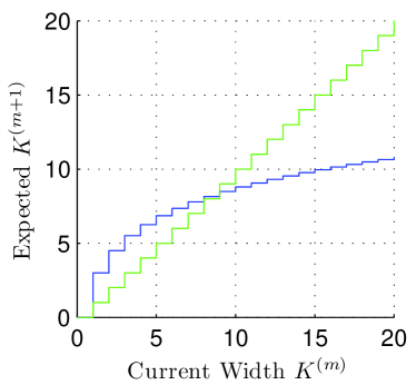
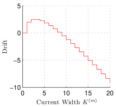
In such a Markov chain, this requirement is equivalent to the statement that the chain has an equilibrium distribution when conditioned on nonabsorption (has a quasi-stationary distribution) (Seneta and Vere-Jones, 1966). For countably-infinite state spaces, a Markov chain has a (quasi-) stationary distribution if it is positive-recurrent, which is the property that there is a finite expected time between consecutive visits to any state. Positive recurrency can be shown by proving the Foster–Lyapunov stability criterion (FLSC) (Fayolle et al., 2008). Taken together, satisfying the FLSC for the Markov chain with transition probabilities given by Eqn 2 demonstrates that eventually the CIBP will reach a restaurant in which the customers try no new dishes. We do this by showing that if $K^{(m)}$ is large enough, the expected $K^{(m+1)}$ is smaller than $K^{(m)}$.

The FLSC requires a Lyapunov function ${\mathcal{L}(k):\mathbb{N}^{+}\to\mathbb{R}\geq 0}$, with which we define the drift function:

$$\mathbb{E}_{k|K^{(m)}}[\mathcal{L}(k)-\mathcal{L}(K^{(m)})] =\sum^{\infty}_{k=1}p(K^{(m+1)}=k\,|\,K^{(m)})(\mathcal{L}(k)-\mathcal{L}(K^{(m)})).$$

The drift is the expected change in $\mathcal{L}(k)$. If there is a $K^{(m)}$ above which all drifts are negative, then the Markov chain satisfies the FLSC and is positive-recurrent. In the CIBP, this is satisfied for ${\mathcal{L}(k)=k}$. That the drift eventually becomes negative can be seen by the fact that

$$\mathbb{E}_{k|K^{(m)}}[\mathcal{L}(k)] =\lambda(K^{(m)}\,;\,\alpha,\beta)$$

is $O(\ln K^{(m)})$ and ${\mathbb{E}_{k|K^{(m)}}[\mathcal{L}(K^{(m)})]=K^{(m)}}$ is $O(K^{(m)})$. Figures 2b and 2c show a schematic of this idea.

(a) $\alpha=1$, $\beta=1$

(b) $\alpha=1$, $\beta=\frac{1}{2}$

(c) $\alpha=\frac{1}{2}$, $\beta=1$

(d) $\alpha=1$, $\beta=2$

(e) $\alpha=\frac{3}{2}$, $\beta=1$

Figure 3: Samples from the CIBP-based prior on network structures, with five visible units.

3.3 The CIBP as a prior on the structure of an infinite belief network

The CIBP can be used as a prior on the sequence ${\boldsymbol{Z}^{(0)},\boldsymbol{Z}^{(1)},\boldsymbol{Z}^{(2)},\cdots}$ from Section 2, to allow an infinite sequence of infinitely-wide hidden layers. As before, there are $K^{(0)}$ visible units. The edges between the first hidden layer and the visible layer are drawn according to the restaurant metaphor. This yields a finite number of units in the first hidden layer, denoted $K^{(1)}$ as before. These units are now treated as the visible units in another IBP-based network. While this recurses infinitely deep, only a finite number of units are ancestors of the visible units. Figure 3 shows several samples from the prior for different parameterizations. Only connected units are shown in the figure.

The parameters $\alpha$ and $\beta$ govern the expected width and sparsity of the network at each level. The expected in-degree of each unit (number of parents) is $\alpha$ and the expected out-degree (number of children) is ${K/\sum^{K}_{k=1}\frac{\beta}{\beta+k-1}}$, for $K$ units used in the layer below. For clarity, we have presented the CIBP results with $\alpha$ and $\beta$ fixed at all depths; however, this may be overly restrictive. For example, in an image recognition problem we would not expect the sparsity of edges mapping low-level features to pixels to be the same as that for high-level features to low-level features. To address this, we allow $\alpha$ and $\beta$ to vary with depth, writing $\alpha^{(m)}$ and $\beta^{(m)}$. The CIBP terminates with probability one as long as there exists some finite upper bound for $\alpha^{(m)}$ and $\beta^{(m)}$ for all $m$.

3.4 Priors on other parameters

Other parameters in the model also require prior distributions and we use these priors to tie parameters together according to layer. We assume that the weights in layer $m$ are drawn independently from Gaussian distributions with mean $\mu^{(m)}_{w}$ and precision $\rho^{(m)}_{m}$. We assume a similar layer-wise prior for biases with parameters $\mu^{(m)}_{\gamma}$ and $\rho^{(m)}_{\gamma}$. We use layer-wise gamma priors on the $\nu^{(m)}_{k}$, with parameters $a^{(m)}$ and $b^{(m)}$. We tie these prior parameters together with global normal-gamma hyperpriors for the weight and bias parameters, and gamma hyperpriors for the precision parameters.

4 Inference

We have so far described a prior on belief network structure and parameters, along with likelihood functions for unit activation. The inference task in this model is to find the posterior distribution over the structure and the parameters of the network, having seen $N$ $K^{(0)}$-dimensional vectors ${\{\boldsymbol{x}_{n}\in(-1,1)^{K^{(0)}}\}^{N}_{n=1}}$. This posterior distribution is complex, so we use Markov chain Monte Carlo (MCMC) to draw samples from ${p(\{\boldsymbol{Z}^{(m)},\boldsymbol{W}^{(m)}\}^{\infty}_{m},\{\boldsymbol{\gamma}^{(m)},\boldsymbol{\nu}^{(m)}\}^{\infty}_{m},\{\boldsymbol{x}_{n}\}^{N}_{n})}$, which, for fixed $\{\boldsymbol{x}_{n}\}^{N}_{n}$, is proportional to the posterior distribution. This joint distribution requires marginalizing over the states of the hidden units that led to each of the $N$ observations. The values of these hidden units are denoted $\{\{\boldsymbol{u}^{(m)}_{n}\}^{\infty}_{m=1}\}^{N}_{n=1}$, and we augment the Markov chain to include these as well.

In general, one would not expect that a distribution on infinite networks would yield tractable inference. However, in our construction, conditioned on the sequence ${\boldsymbol{Z}^{(1)},\boldsymbol{Z}^{(2)},\cdots}$, almost all of the infinite number of units are independent. Due to this independence, they trivially marginalize out of the model’s joint distribution and we can restrict inference only to those units that are ancestors of the visible units. Of course, since this trivial marginalization only arises from the $\boldsymbol{Z}^{(m)}$ matrices, we must also have a distribution on infinite binary matrices that allows exact marginalization of all the uninstantiated edges. The row-wise and column-wise exchangeability properties of the IBP are what allows the use of infinite matrices. The bottom-up conditional structure of the CIBP allows an infinite number of these matrices.

To simplify notation, we will use $\boldsymbol{\Omega}$ for the aggregated state of the model variables, i.e. ${\boldsymbol{\Omega}\!=\!(\{\boldsymbol{Z}^{(m)},\boldsymbol{W}^{(m)},\{\boldsymbol{u}^{(m)}_{n}\}^{N}_{n=1}\}^{\infty}_{m=1},\{\boldsymbol{\gamma}^{(m)},\boldsymbol{\nu}^{(m)}\}^{\infty}_{m=0},\{\boldsymbol{x}_{n}\}^{N}_{n=1})}$. Given the hyperparameters, we can then write the joint distribution as

$$p(\boldsymbol{\Omega})=\left(p(\boldsymbol{\gamma}^{(0)})\,p(\boldsymbol{\nu}^{(0)})\prod^{K^{(0)}}_{k=1}\prod^{N}_{n=1}p(x_{k,n}\,|\,y^{(0)}_{k,n},\nu^{(0)}_{k})\right)\\ \times\left(\prod^{\infty}_{m=1}p(\boldsymbol{W}^{(m)})\,p(\boldsymbol{\gamma}^{(m)})\,p(\boldsymbol{\nu}^{(m)})\prod^{K^{(m)}}_{k=1}\prod^{N}_{n=1}p(u^{(m)}_{k,n}\,|\,y^{(m)}_{k,n},\nu^{(m)}_{k})\right).$$ (3)

Although this distribution involves several infinite sets, it is possible to sample from the relevant parts of the posterior. We do this by MCMC, updating part of the model, while conditioning on the rest. In particular, conditioning on the binary matrices ${\{\boldsymbol{Z}^{(m)}\}^{\infty}_{m=1}}$, which define the structure of the network, inference becomes exactly as it would be in a finite belief network.

4.1 Sampling from the hidden unit states

Since we cannot easily integrate out the hidden units, it is necessary to explicitly represent them and sample from them as part of the Markov chain. As we are conditioning on the network structure, it is only necessary to sample the units that are ancestors of the visible units. Frey (1997) proposed a slice sampling scheme for the hidden unit states but we have been more successful with a specialized independence-chain variant of multiple-try Metropolis–Hastings (Liu et al., 2000). Our method proposes several ($\approx 5$) possible new unit states from the activation distribution and selects from among them (or rejects them all) according to the likelihood imposed by its children. As this operation can be executed in parallel by tools such as Matlab, we have seen significantly better mixing performance by wall-clock time than the slice sampler.

4.2 Sampling from the weights and biases

Given that a directed edge exists, we sample the posterior distribution over its weight. Conditioning on the rest of the model, the NLGBN results in a convenient Gaussian form for the distribution on weights so that we can Gibbs update them using a Gaussian with parameters

$$\mu^{\sf{w-post}}_{m,k,k^{\prime}} \!=\!\frac{\rho^{(m)}_{w}\!\mu^{(m)}_{w}\!\!+\!\nu^{(m\!-\!1)}_{k}\!\sum_{n}\!\!u^{(m)}_{n,k^{\prime}}(\sigma^{-\!1}(u^{(m\!-\!1)}_{k})\!-\!\xi^{(m)}_{n,k,k^{\prime}})}{\rho^{(m)}_{w}+\nu^{(m-1)}_{k}\sum_{n}(u^{(m)}_{n,k^{\prime}})^{2}}$$ (4)

$$\rho^{\sf{w-post}}_{m,k,k^{\prime}} \!=\!\rho^{(m)}_{w}+\nu^{(m-1)}_{k}\sum_{n}(u^{(m)}_{n,k^{\prime}})^{2},$$ (5)

where

$$\xi^{(m)}_{n,k,k^{\prime}} =\gamma^{(m-1)}_{k}+\sum_{k^{\prime\prime}\neq k^{\prime}}Z^{(m)}_{k,k^{\prime\prime}}W^{(m)}_{k,k^{\prime\prime}}u^{(m)}_{n,k^{\prime\prime}}.$$ (6)

The bias $\gamma^{(m)}_{k}$ can be similarly sampled from a Gaussian distribution with parameters

$$\mu^{\gamma\sf{-post}}_{m,k} =\frac{\rho^{(m)}_{\gamma}\mu^{(m)}_{\gamma}+\nu^{(m)}_{k}\sum^{N}_{n=1}(\sigma^{-1}(u^{(m)}_{n,k})-\chi^{(m)}_{n,k})}{\rho^{(m)}_{\gamma}+N\nu^{(m)}_{k}}$$ (7)

$$\rho^{\gamma\sf{-post}}_{m,k} =\rho^{(m)}_{\gamma}+N\nu^{(m)}_{k}$$ (8)

where

$$\chi^{(m)}_{n,k} =\sum^{K^{(m+1)}}_{k^{\prime}=1}Z^{(m+1)}_{k,k^{\prime}}W^{(m+1)}_{k,k^{\prime}}u^{(m+1)}_{n,k^{\prime}}.$$ (9)

4.3 Sampling from the activation variances

We use the NLGBN model to gain the ability to change the mode of unit behaviors between discrete and continuous representations. This corresponds to sampling from the posterior distributions over the $\nu^{(m)}_{k}$. With a conjugate prior, the new value can be sampled from a gamma distribution with parameters

$$a^{\nu\sf{-post}}_{m,k} =a^{(m)}_{\nu}+N/2$$ (10)

$$b^{\nu\sf{-post}}_{m,k} =b^{(m)}_{\nu}+\frac{1}{2}\sum^{N}_{n=1}(\sigma^{-1}(u^{(m)}_{n,k})-y^{(m)}_{k})^{2}.$$ (11)

4.4 Sampling from the structure

A model for infinite belief networks is only useful if it is possible to perform inference. The appeal of the CIBP prior is that it enables construction of a tractable Markov chain for inference. To do this sampling, we must add and remove edges from the network, consistent with the posterior equilibrium distribution. When adding a layer, we must sample additional layerwise model components. When introducing an edge, we must draw a weight for it from the prior. If this new edge introduces a previously-unseen hidden unit, we must draw a bias for it and also draw its deeper cascading connections from the prior. Finally, we must sample the $N$ new hidden unit states from any new unit we introduce.

We iterate over each layer that connects to the visible units. Within each layer ${m\geq 0}$, we iterate over the connected units. Sampling the edges incident to the $k$th unit in layer $m$ has two phases. First, we iterate over each connected unit in layer ${m+1}$, indexed by $k^{\prime}$. We calculate $\eta^{(m)}_{-k,k^{\prime}}$, which is the number of nonzero entries in the $k^{\prime}$th column of $\boldsymbol{Z}^{(m+1)}$, excluding any entry in the $k$th row. If $\eta^{(m)}_{-k,k^{\prime}}$ is zero, we call the unit $k^{\prime}$ a singleton parent, to be dealt with in the second phase. If $\eta^{(m)}_{-k,k^{\prime}}$ is nonzero, we introduce (or keep) the edge from unit $u^{(m+1)}_{k^{\prime}}$ to $u^{(m)}_{k}$ with Bernoulli probability

$$p(Z^{(m+1)}_{k,k^{\prime}}=1\,|\,\boldsymbol{\Omega}\backslash Z^{(m+1)}_{k,k^{\prime}})=\frac{1}{\mathcal{Z}}\left(\!\frac{\eta^{(m)}_{-k,k^{\prime}}}{K^{(m)}\!+\!\beta^{(m)}\!-\!1}\!\right)\\ \times\prod^{N}_{n=1}p(u^{(m)}_{n,k}\,|\,Z^{(m+1)}_{k,k^{\prime}}=1,\boldsymbol{\Omega}\backslash Z^{(m)}_{k,k^{\prime}})$$

$$p(Z^{(m+1)}_{k,k^{\prime}}=0\,|\,\boldsymbol{\Omega}\backslash Z^{(m+1)}_{k,k^{\prime}})=\frac{1}{\mathcal{Z}}\left(\!1\!-\!\frac{\eta^{(m)}_{-k,k^{\prime}}}{K^{(m)}\!+\!\beta^{(m)}\!-\!1}\!\right)\\ \times\prod^{N}_{n=1}p(u^{(m)}_{n,k}\,|\,Z^{(m+1)}_{k,k^{\prime}}=0,\boldsymbol{\Omega}\backslash Z^{(m+1)}_{k,k^{\prime}}),$$

where $\mathcal{Z}$ is the appropriate normalization constant.

In the second phase, we consider deleting connections to singleton parents of unit $k$, or adding new singleton parents. We do this via a Metropolis–Hastings operator using a birth/death process. If there are currently $K_{\circ}$ singleton parents, then with probability $1/2$ we propose adding a new one by drawing it recursively from deeper layers, as above. We accept the proposal to insert a connection to this new parent unit with M–H acceptance ratio

$$a_{\sf{mh-insert}} =\frac{\alpha^{(m)}\beta^{(m)}}{(K_{\circ}\!+\!1)^{2}(\beta^{(m)}\!+\!K^{(m)}\!-\!1)}\prod^{N}_{n=1}\frac{p(u^{(m)}_{n,k}\,|\,Z^{(m+1)}_{k,j}\!\!=\!1,\boldsymbol{\Omega}\backslash Z^{(m+1)}_{k,j})}{p(u^{(m)}_{n,k}\,|\,Z^{(m+1)}_{k,j}\!\!=\!0,\boldsymbol{\Omega}\backslash Z^{(m+1)}_{k,j})}.$$

If we do not propose to insert a unit and ${K_{\circ}\geq 0}$, then with probability $1/2$ we select uniformly from among the singleton parents of unit $k$ and propose removing the connection to it. We accept the proposal to remove the $j$th one with M–H acceptance ratio

$$a_{\sf{mh-remove}} =\frac{K_{\circ}^{2}(\beta^{(m)}\!+\!K^{(m)}\!-\!1)}{\alpha^{(m)}\beta^{(m)}}\prod^{N}_{n=1}\frac{p(u^{(m)}_{n,k}\,|\,Z^{(m+1)}_{k,j}\!\!=\!0,\boldsymbol{\Omega}\backslash Z^{(m+1)}_{k,j})}{p(u^{(m)}_{n,k}\,|\,Z^{(m+1)}_{k,j}\!\!=\!1,\boldsymbol{\Omega}\backslash Z^{(m+1)}_{k,j})}.$$

After these phases, chains of units that are not ancestors of the visible units can be discarded. Notably, this birth/death operator samples from the IBP posterior with a non-truncated equilibrium distribution, even without conjugacy. Unlike the stick-breaking approach of Teh et al. (2007), it allows use of the two-parameter IBP, which is important to this model.

4.5 Sampling From CIBP Hyperparameters

When applying this model to data, it is infrequently the case that we would have a good a priori idea of what the appropriate IBP parameters should be. These control the width and sparsity of the network and while we might have good initial guesses for the lowest layer, in general we would like to infer $\{\alpha^{(m)},\beta^{(m)}\}$ as part of the larger inference procedure. This is straightforward in the fully-Bayesian MCMC procedure we have constructed, and it does not differ markedly from hyperparameter inference in standard IBP models when conditioning on $\boldsymbol{Z}^{(m)}$. As in some other nonparametric models (e.g. Tokdar (2006) and Rasmussen and Williams (2006)), we have found that light-tailed priors on the hyperparameters helps ensure that the model stays in reasonable states.

(a)

(b)

(c)

(d)

Figure 4: Olivetti faces a) Test images on the left, with reconstructed bottom halves on the right. b) Sixty features learned in the bottom layer, where black shows absence of an edge. Note the learning of sparse features corresponding to specific facial structures such as mouth shapes, noses and eyebrows. c) Raw predictive fantasies. d) Feature activations from individual units in the second hidden layer.

5 Reconstructing Images

We applied the model and MCMC-based inference procedure to three image data sets: the Olivetti faces, the MNIST digits and the Frey faces. We used these data to analyze the structures and sparsity that arise in the model posterior. To get a sense of the utility of the model, we constructed a missing-data problem using held-out images from each set. We removed the bottom halves of the test images and asked the model to reconstruct the missing data, conditioned on the top half. The prediction itself was done by integrating out the parameters and structure via MCMC.

Olivetti Faces

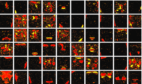
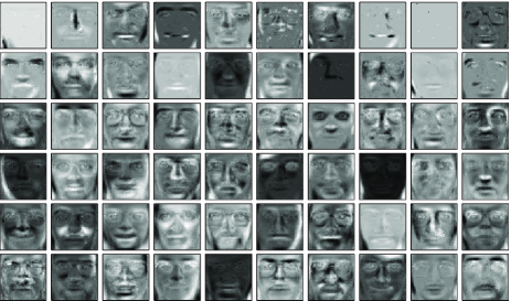
The Olivetti faces data (Samaria and Harter, 1994) consists of 400 ${64\times 64}$ grayscale images of the faces of 40 distinct subjects. We divided these into 350 test data and 50 training data, selected randomly. This data set is an appealing test because it has few examples, but many dimensions. Figure 4a shows six bottom-half test set reconstructions on the right, compared to the ground truth on the left. Figure 4b shows a subset of sixty weight patterns from a posterior sample of the structure, with black indicating that no edge is present from that hidden unit to the visible unit (pixel). The algorithm is clearly assigning hidden units to specific and interpretable features, such as mouth shapes, the presence of glasses or facial hair, and skin tone, while largely ignoring the rest of the image. Figure 4c shows ten pure fantasies from the model, easily generated in a directed acyclic belief network. Figure 4d shows the result of activating individual units in the second hidden layer, while keeping the rest unactivated, and propagating the activations down to the visible pixels. This provides an idea of the image space spanned by the principal components of these deeper units. A typical posterior network had three hidden layers, with about 70 units in each layer.

(a)

(b)

(c)

(d)

Figure 5: MNIST Digits a) Eight pairs of test reconstructions, with the bottom half of each digit missing. The truth is the left image in each pair. b) 120 features learned in the bottom layer, where black indicates that no edge exists. c) Activations in pixel space resulting from activating individual units in the deepest layer. d) Samples from the posterior of $\boldsymbol{Z}^{(0)}$, $\boldsymbol{Z}^{(1)}$ and $\boldsymbol{Z}^{(2)}$ (transposed).

MNIST Digit Data

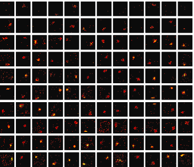
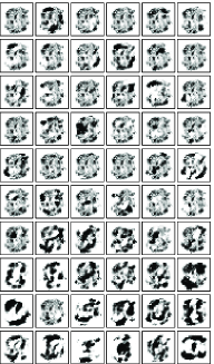
We used a subset of the MNIST handwritten digit data (LeCun et al., 1998) for training, consisting of 50 ${28\times 28}$ examples of each of the ten digits. We used an additional ten examples of each digit for test data. In this case, the lower-level features are extremely sparse, as shown in Figure 5b, and the deeper units are simply activating sets of blobs at the pixel level. This is shown also by activating individual units at the deepest layer, as shown in Figure 5c. Test reconstructions are shown in Figure 5a. A typical network had three hidden layers, with approximately 120 in the first, 100 in the second and 70 in the third. The binary matrices $\boldsymbol{Z}^{(0)}$, $\boldsymbol{Z}^{(1)}$, and $\boldsymbol{Z}^{(2)}$ are shown in Figure 5d.

Frey Faces

The Frey faces data are 1965 ${20\times 28}$ grayscale video frames of a single face with different expressions. We divided these into 1865 training data and 100 test data, selected randomly. While typical posterior samples of the network again typically used three hidden layers, the networks for these data tended to be much wider and more densely connected. In the bottom layer, as shown in Figure 6b, a typical hidden unit would connect to many pixels. We attribute this to global correlation effects from every image only coming from a single person. Typical widths were 260 units, 120 units in the second hidden layer, and 35 units in the deepest layer.

(a)

(b)

Figure 6: Frey faces a) Eight pairs of test reconstructions, with the bottom half of each face missing. The truth is the left image in each pair. b) 260 features learned in the bottom layer, where black indicates that no edge exists.

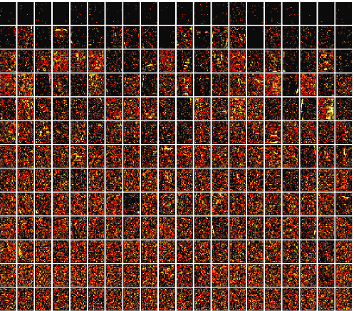
In all three experiments, our MCMC sampler appeared to mix well and begins to find reasonable reconstructions after a few hours of CPU time. It is interesting to note that the learned sparse connection patterns in $\boldsymbol{Z}^{(0)}$ varied from local (MNIST), through intermediate (Olivetti) to global (Frey), despite identical hyperpriors on the IBP parameters. This strongly suggests that flexible priors on structures are needed to adequately capture the statistics of different data sets.

6 Discussion

This paper unites two areas of research—nonparametric Bayesian methods and deep belief networks—to provide a novel nonparametric perspective on the general problem of learning the structure of directed deep belief networks with hidden units.

We addressed three outstanding issues that surround deep belief networks. First, we allowed the units to have different operating regimes and infer appropriate local representations that range from discrete binary behavior to nonlinear continuous behavior. Second, we provided a way for a deep belief network to contain an arbitrary number of hidden units arranged in an arbitrary number of layers. This structure enables the hidden units to have nontrivial joint distributions. Third, we presented a method for inferring the appropriate directed graph structure of deep belief network. To address these issues, we introduced a novel cascading extension to the Indian buffet process—the cascading Indian buffet process (CIBP)—and proved convergence properties that make it useful as a Bayesian prior distribution for a sequence of infinite binary matrices.

This work can be viewed as an infinite multilayer generalization of the density network (MacKay, 1995), and also as part of a more general literature of learning structure in probabilistic networks. With a few exceptions (e.g., Ramachandran and Mooney (1998); Friedman (1998); Elidan et al. (2000); Beal and Ghahramani (2006)), most previous work on learning the structure of belief networks has focused on the case where all units are observed (Buntine, 1991; Heckerman et al., 1995; Friedman and Koller, 2003; Koivisto and Sood, 2004). The framework presented in this paper not only allows for an unbounded number of hidden units, but fundamentally couples the model for the number and behavior of the units with the nonparametric model for the structure of the infinite directed graph. Rather than comparing structures by evaluating marginal likelihoods of different models, our nonparametric approach makes it possible to do inference in a single model with an unbounded number of units and layers, thereby learning effective model complexity. This approach is more appealing both computationally and philosophically.

There are a variety of future research paths that can potentially stem from the model we have presented here. As we have presented it, we do not expect that our MCMC-based unsupervised inference scheme will be competitive on supervised tasks with extensively-tuned discriminative models based on variants of maximum-likelihood learning. However, we believe that this model can inform choices for network depth, layer size and edge structure in such networks and will inspire further research into flexible nonparametric network models.

Acknowledgements

The authors wish to thank Brendan Frey, David MacKay, Iain Murray and Radford Neal for valuable discussions. RPA is funded by the Canadian Institute for Advanced Research.

Appendix A Proof of General CIBP Termination

In the main paper, we discussed that the cascading Indian buffet process for fixed and finite $\alpha$ and $\beta$ eventually reaches a restaurant in which the customers choose no dishes. Every deeper restaurant also has no dishes. Here we show a more general result, for IBP parameters that vary with depth, written $\alpha^{(m)}$ and $\beta^{(m)}$.

Let there be an inhomogeneous Markov chain $\mathcal{M}$ with state space $\mathbb{N}$. Let $m$ index time and let the state at time $m$ be denoted $K^{(m)}$. The initial state $K^{(0)}$ is finite. The probability mass function describing the transition distribution for $\mathcal{M}$ at time $m$ is given by

$$p(K^{(m+1)}=k\,|\,K^{(m)},\alpha^{(m)},\beta^{(m)})=\\ \frac{1}{k!}\exp\left\{-\alpha^{(m)}\sum^{K^{(m)}}_{k^{\prime}=1}\frac{\beta^{(m)}}{k^{\prime}+\beta^{(m)}-1}\right\}\left(\alpha^{(m)}\sum^{K^{(m)}}_{k^{\prime}=1}\frac{\beta^{(m)}}{k^{\prime}+\beta^{(m)}-1}\right).$$ (12)

Theorem A.1.

If there exists some ${\bar{\alpha}<\infty}$ and ${\bar{\beta}<\infty}$ such that $\forall m$, ${\alpha^{(m)}<\bar{\alpha}}$ and ${\beta^{(m)}<\bar{\beta}}$, then ${\lim_{m\to\infty}p(K^{(m)}=0)=1}$.

Proof.

Let $\mathbb{N}^{+}$ be the positive integers. The $\mathbb{N}^{+}$ are a communicating class for the Markov chain (it is possible to eventually reach any member of the class from any other member) and each $K^{(m)}\in\mathbb{N}^{+}$ has a nonzero probability of transitioning to the absorbing state ${K^{(m+1)}=0}$, i.e. ${p(K^{(m+1)}=0\,|\,K^{(m)})>0}$, $\forall K^{(m)}$. If, conditioned on nonabsorption, the Markov chain has a stationary distribution (is quasi-stationary), then it reaches absorption in finite time with probability one. Heuristically, this is the requirement that, conditioned on having not yet reached a restaurant with no dishes, the number of dishes in deeper restaurants will not explode.

The quasi-stationary condition can be met by showing that $\mathbb{N}^{+}$ are positive recurrent states. We use the Foster–Lyapunov stability criterion (FLSC) to show positive-recurrency of $\mathbb{N}^{+}$. The FLSC is met if there exists some function ${\mathcal{L}(\cdot):\mathbb{N}^{+}\to\mathbb{R}^{+}}$ such that for some $\epsilon>0$ and some finite $B\in\mathbb{N}^{+}$,

$$\sum^{\infty}_{k=1}p(K^{(m+1)}=k\,|\,K^{(m)})\,\left(\mathcal{L}(k)-\mathcal{L}(K^{(m)})\right) <-\epsilon\text{ for }K^{(m)}>B$$ (13)

$$\sum^{\infty}_{k=1}p(K^{(m+1)}=k\,|\,K^{(m)})\,\mathcal{L}(k) <\infty\text{ for }K^{(m)}\leq B.$$ (14)

For Lyapunov function $\mathcal{L}(k)=k$, the first condition is equivalent to

$$\left(\alpha^{(m)}\sum^{K^{(m)}}_{k=1}\frac{\beta^{(m)}}{k+\beta^{(m)}-1}\right)-K^{(m)}<-\epsilon.$$ (15)

We observe that

$$\alpha^{(m)}\sum^{K^{(m)}}_{k=1}\frac{\beta^{(m)}}{k+\beta^{(m)}-1} <\bar{\alpha}\sum^{K^{(m)}}_{k=1}\frac{\bar{\beta}}{k+\bar{\beta}-1},$$ (16)

for all $K^{(m)}>0$. Thus, the first condition is satisfied for any $B$ that satisfies the condition for $\bar{\alpha}$ and $\bar{\beta}$. That such a $B$ exists for any finite $\bar{\alpha}$ and $\bar{\beta}$ can be seen by the equivalent condition

$$\left(\bar{\alpha}\sum^{K^{(m)}}_{k=1}\frac{\bar{\beta}}{k+\bar{\beta}-1}\right)-K^{(m)}<-\epsilon\text{ for }K^{(m)}>B.$$ (17)

As the first term is roughly logarithmic in $K^{(m)}$, there exists some finite $B$ that satisfies this inequality. The second FLSC condition is trivially satisfied by the observation that Poisson distributions have a finite mean. ∎

References

- Beal and Ghahramani [2006] M. J. Beal and Z. Ghahramani. Variational Bayesian learning of directed graphical models with hidden variables. Bayesian Analysis, 1(4):793–832, 2006.
- Buntine [1991] W. Buntine. Theory refinement on Bayesian networks. In Proc. of the 7th Annual Conference on Uncertainty in Artificial Intelligence, pages 52–60, 1991.
- Elidan et al. [2000] G. Elidan, N. Lotner, N. Friedman, and D. Koller. Discovering hidden variables: A structure-based approach. In Advances in Neural Information Processing Systems 13, 2000.
- Fayolle et al. [2008] G. Fayolle, V. A. Malyshev, and M. V. Menshikov. Topics in the Constructive Theory of Countable Markov Chains. Cambridge University Press, Cambridge, UK, 2008.
- Frey [1997] B. J. Frey. Continuous sigmoidal belief networks trained using slice sampling. In Adv. in Neural Information Processing Systems 9, 1997.
- Frey and Hinton [1999] B. J. Frey and G. E. Hinton. Variational learning in nonlinear Gaussian belief networks. Neural Computation, 11(1):193–213, 1999.
- Friedman [1998] N. Friedman. The Bayesian structural EM algorithm. In Proceedings of the 14th Annual Conference on Uncertainty in Artificial Intelligence, 1998.
- Friedman and Koller [2003] N. Friedman and D. Koller. Being Bayesian about network structure: A Bayesian approach to structure discovery in Bayesian networks. Machine Learning, 50(1-2):95–125, 2003.
- Ghahramani et al. [2007] Z. Ghahramani, T. L. Griffiths, and P. Sollich. Bayesian nonparametric latent feature models. In Bayesian Statistics 8, pages 201–226. Oxford University Press, Oxford, 2007.
- Griffiths and Ghahramani [2006] T. L. Griffiths and Z. Ghahramani. Infinite latent feature models and the Indian buffet process. In Advances in Neural Information Processing Systems 18, pages 475–482, 2006.
- Heckerman et al. [1995] D. Heckerman, D. Geiger, and D. M. Chickering. Learning Bayesian networks: The combination of knowledge and statistical data. Machine Learning, 20(3):197–243, 1995.
- Hinton and Salakhutdinov [2006] G. E. Hinton and R. Salakhutdinov. Reducing the dimensionality of data with neural networks. Science, 313(5786):504–507, 2006.
- Hinton et al. [2006] G. E. Hinton, S. Osindero, and Y.-W. Teh. A fast learning algorithm for deep belief nets. Neural Computation, 18(7):1527–1554, July 2006.
- Koivisto and Sood [2004] M. Koivisto and K. Sood. Exact Bayesian structure discovery in Bayesian networks. Journal of Machine Learning Research, 5:549–573, 2004.
- Le Roux and Bengio [2008] N. Le Roux and Y. Bengio. Representational power of restricted Boltzmann machines and deep belief networks. Neural Computation, 20(6):1631–1649, 2008.
- LeCun et al. [1998] Y. LeCun, L. Bottou, Y. Bengio, and P. Haffner. Gradient-based learning applied to document recognition. Proc. of the IEEE, 86(11):2278–2324, 1998.
- Liu et al. [2000] J. S. Liu, F. Liang, and W. H. Wong. The use of multiple-try method and local optimization in Metropolis sampling. Journal of the American Statistical Association, 95(449):121–134, 2000.
- MacKay [1995] D. J. C. MacKay. Bayesian neural networks and density networks. Nuclear Instruments and Methods in Physics Research, Section A, 354(1):73–80, 1995.
- Neal [1992] R. M. Neal. Connectionist learning in belief networks. Artificial Intelligence, 56:71–113, July 1992.
- Pearl [1988] J. Pearl. Probabalistic Reasoning in Intelligent Systems: Networks of Plausible Inference. Morgan Kaufmann, San Mateo, CA, 1988.
- Ramachandran and Mooney [1998] S. Ramachandran and R. J. Mooney. Theory refinement of Bayesian networks with hidden variables. In Proceedings of the 15th International Conference on Machine Learning, pages 454–462, 1998.
- Rasmussen and Williams [2006] C. E. Rasmussen and C. K. I. Williams. Gaussian Processes for Machine Learning. MIT Press, Cambridge, MA, 2006.
- Samaria and Harter [1994] F. S. Samaria and A. C. Harter. Parameterisation of a stochastic model for human face identification. In Proceedings of the 2nd IEEE workshop on Applications of Computer Vision, 1994.
- Seneta and Vere-Jones [1966] E. Seneta and D. Vere-Jones. On quasi-stationary distributions in discrete-time Markov chains with a denumerable infinity of states. Journal of Applied Probability, 3(2):403–434, December 1966.
- Teh et al. [2007] Y.-W. Teh, D. Görür, and Z. Ghahramani. Stick-breaking construction for the Indian buffet process. In Proc. of the International Conference on Artificial Intelligence and Statistics, volume 11, 2007.
- Tokdar [2006] S. T. Tokdar. Exploring Dirichlet Mixture and Logistic Gaussian Process Priors in Density Estimation, Regression and Sufficient Dimension Reduction. PhD thesis, Purdue University, August 2006.
- Wood et al. [2006] F. Wood, T. L. Griffiths, and Z. Ghahramani. A non-parametric Bayesian method for inferring hidden causes. In Proceedings of the 22nd Conference in Uncertainty in Artificial Intelligence, 2006.