Inferring Multiple Graphical Structures

Abstract

Gaussian Graphical Models provide a convenient framework for representing dependencies between variables. Recently, this tool has received a high interest for the discovery of biological networks. The literature focuses on the case where a single network is inferred from a set of measurements, but, as wetlab data is typically scarce, several assays, where the experimental conditions affect interactions, are usually merged to infer a single network. In this paper, we propose two approaches for estimating multiple related graphs, by rendering the closeness assumption into an empirical prior or group penalties. We provide quantitative results demonstrating the benefits of the proposed approaches. The methods presented in this paper are embeded in the R package simone from version 1.0-0 and later.

, , . label=e1][julien.chiquet,christophe.ambroise]@genopole.cnrs.fr label=e3]yves.grandvalet@utc.fr label=u]http://stat.genopole.cnrs.fr

1 Motivations

Systems biology provides a large amount of data sets that aim to understand the complex relationships existing between the molecular entities that drive any biological process. Depending on the molecule of interest, various networks can be inferred, e.g., gene-to-gene regulation networks or protein-protein interaction networks. The basic idea is to consider that if two molecules interact, a statistical dependency between their expression should be observed.

A convenient model of multivariate dependence patterns is Gaussian Graphical Modeling (GGM). In this framework, a multidimensional Gaussian variable is characterized by the so-called concentration matrix, where conditional independence between pairs of variables is characterized by a zero entry. This matrix may be represented by an undirected graph, where each vertex represents a variable, and an edge connects two vertices if the corresponding pair of random variables are dependent, conditional on the remaining variables.

Merging different experimental conditions from wetlab data is a common practice in GGM-based inference methods (Toh and Horimoto 2002, Schäfer and Strimmer 2005). This process enlarges the number of observations available for inferring interactions. However, GGMs assume that the observed data form an independent and identically distributed (i.i.d.) sample. In the aforementioned paradigm, assuming that the merged data is drawn from a single Gaussian component is obviously wrong, and is likely to have detrimental side effects in the estimation process.

In this paper, we propose to remedy this problem by estimating multiple GGMs, each of whom matching different modalities of the same set of variables, which correspond here to the different experimental conditions. As the distributions of these modes have strong commonalities, we propose to estimate these graphs jointly. Considering several tasks at a time has been attracting much attention in the machine learning literature, where the generic problem is usually referred to as “multi-task learning” (Caruana 1997). Efron (2009) used the terms “indirect evidence” and “learning from the experience of others” for similar ideas. The principle is to learn an inductive bias, whose role is to stabilize the estimation process, hopefully enabling more accurate predictions in small sample size regimes (Baxter 2000). The techniques comprise the empirical and hierarchical Bayes methodologies and regularization schemes (see Argyriou et al. 2008, for example), which may be interpreted as approximations to the latter. Here, we will mainly follow the penalty-based approach to leverage the inference of several related graphs towards a common pattern.

A typical example of this problem arises when inferring gene interactions from data measured on slightly different stem cells, such as wild and mutant. It is reasonable to assume that most, though not all, interactions will be common to both types of cells. The line of attack we propose alleviates the difficulties arising from the scarcity of data in each experimental condition by coupling the estimation problems. Our first proposal biases the estimation of the concentration matrices towards a common value. Our second proposition focuses on the similarities in the sparsity pattern that are more directly related to the graph itself. We propose the Cooperative-LASSO, which builds on the Group-LASSO (Yuan and Lin 2006) to favor solutions with a common sparsity pattern, but encodes a further preference towards solutions with similar sign patterns, thus preserving the type of co-regulation (positive or negative) across assays.

To our knowledge, the present work is the first to exploit the multi-task learning framework for learning GGMs. However, coupling the estimation of several networks has recently been investigated for Markov random fields, in the context of time-varying networks. Kolar et al. (2009) propose two specific constraints, one for smooth variations over time, the other one for abrupt changes. Their penalties are closer to the Fused-LASSO and total variations penalties than to the group penalties proposed here.

2 Network Inference with GGM

In the GGM framework, we aim to infer the graph of conditional dependencies among the $p$ variables of a vector $X$ from independent observations $(X^{1},\dots,X^{n})$. We assume that $X$ is a $p$-dimensional Gaussian random variable $X\sim\mathcal{N}(\mathbf{0}_{p},{\boldsymbol{\Sigma}})$. Let $\mathbf{K}={\boldsymbol{\Sigma}}^{-1}$ be the concentration matrix of the model; the non-zero entries of $K_{ij}$ indicate a conditional dependency between the variables $X_{i}$ and $X_{j}$, and thus define the graph $\mathcal{G}$ of conditional dependencies of $X$.

The GGM approach produces the graph $\mathcal{G}$ from an inferred $\mathbf{K}$. The latter cannot be obtained by maximum likelihood estimation that would typically return a full matrix, and hence a useless fully connected graph. To produce sparse networks, Banerjee et al. (2008) propose to penalize the entries of $\mathbf{K}$ by an $\ell_{1}$-norm. Friedman et al. (2008) latter addressed the very same problem with an elegant algorithm named the graphical-LASSO. Their well-motivated approach produces a sparse, symmetric and positive-definite estimate of the concentration matrix. However, a cruder though more direct approach has been reported to be more accurate in terms of edge detection (Villers et al. 2008, Rocha et al. 2008). This approach, proposed by Meinshausen and Bühlmann (2006) and known as neighborhood selection, determines $\mathcal{G}$ via an iterative estimation of the neighborhood of its nodes. For this purpose, it considers $p$ independent $\ell_{1}$-penalized regression problems. Let $\mathbf{X}$ be the $n\times p$ matrix of stacked observations, whose $k$th row contains $(X^{k})^{\intercal}$. The vertices adjacent to vertex $i$ are estimated by the non-zero elements of $\boldsymbol{\beta}$ solving

$$\min_{\boldsymbol{\beta}\in\mathbb{R}^{p-1}}\frac{1}{n}\left\|\mathbf{X}_{i}-\mathbf{X}_{\backslash i}\boldsymbol{\beta}\right\|_{2}^{2}+\lambda\|\boldsymbol{\beta}\|_{1}\enspace,$$ (1)

where $\mathbf{X}_{i}$ is the $i$th column of $\mathbf{X}$ and $\mathbf{X}_{\backslash i}$ is $\mathbf{X}$ deprived of its $i$th column: the $i$th variable is “explained” by the remaining ones. As the neighborhood of the $p$ variables are selected separately, a post-symmetrization must be applied to manage inconsistencies between edge selections; Meinshausen and Bühlmann suggest AND or OR rules, which are both asymptotically consistent (as $n$ goes to infinity).

Solving the $p$ regression problems (1) may be interpreted as inferring the concentration matrix in a penalized, pseudo maximum likelihood framework, where the joint distribution of $X$ is approximated by the product of the $p$ distributions of each variable conditional on the other ones (Rocha et al. 2008, Ambroise et al. 2009, Ravikumar et al. 2010), that is

$$\mathcal{L}(\mathbf{K}|\mathbf{X})=\sum_{i=1}^{p}\left(\sum_{k=1}^{n}\log\mathbb{P}(X_{i}^{k}|X^{k}_{\backslash i};\mathbf{K}_{i})\right)\enspace,$$

where $X_{\backslash i}^{k}$ is the $k$th realization of the vector $X$ deprived of the $i$th coordinate. Considering the Gaussian assumption on the generation of the data $\mathbf{X}$, the pseudo-log-likelihood admits a compact and simple expression (see derivation in Appendix A.1):

$$\mathcal{L}(\mathbf{K}|\mathbf{X})=\frac{n}{2}\log\det(\mathbf{D})-\frac{n}{2}\mathrm{Tr}\left(\mathbf{D}^{-\frac{1}{2}}\mathbf{K}\mathbf{S}\mathbf{K}\mathbf{D}^{-\frac{1}{2}}\right)\\ -\frac{np}{2}\log(2\pi)\enspace,$$ (2)

where $\mathbf{S}=n^{-1}\mathbf{X}^{\intercal}\mathbf{X}$ is the empirical covariance matrix, and $\mathbf{D}$ is a $p\times p$ diagonal matrix with elements $D_{ii}=K_{ii}$. In the sequel, it will be convenient to use the sufficiency of $\mathbf{S}$ for $\mathbf{K}$, and, by a slight abuse of notations, write $\mathcal{L}(\mathbf{K}|\mathbf{X})=\mathcal{L}(\mathbf{K}|\mathbf{S})$.

Following Banerjee et al. (2008), an $\ell_{1}$ penalty may be added to obtain a sparse estimate of $\mathbf{K}$. Nevertheless, our approach to maximizing the pseudo-log-likelihood is much simpler than the optimization of the log-likelihood proposed by Banerjee et al. (2008). Indeed, as stated formally in the following proposition, maximizing the penalized pseudo-log-likelihood on the set of arbitrary matrices (not constrained to be either symmetric or positive definite) boils down to solving $p$ independent LASSO problems of size $p-1$. Furthermore, for the purpose of discovering the graph structure, additional computational savings are achieved by remarking that $\mathbf{D}$ needs not to be estimated. We thus avoid the iterative scheme of Rocha et al. (2008) alternating optimization with respect to $\mathbf{D}$ and to the off-diagonal elements of $\mathbf{D}^{-1}\mathbf{K}$.

Proposition 1.

Consider the following reordering of the rows and columns of $\mathbf{K}$ and $\mathbf{S}$:

$$\begin{bmatrix}\mathbf{K}_{\backslash i\backslash i}&\mathbf{K}_{i\backslash i}\\ \mathbf{K}_{i\backslash i}^{\intercal}&K_{ii}\\ \end{bmatrix},\quad\begin{bmatrix}\mathbf{S}_{\backslash i\backslash i}&\mathbf{S}_{i\backslash i}\\ \mathbf{S}_{i\backslash i}^{\intercal}&S_{ii}\\ \end{bmatrix}\enspace,$$ (3)

where $\mathbf{K}_{\backslash i\backslash i}$ is matrix $\mathbf{K}$ deprived of its $i$th column and its $i$th line, and where $\mathbf{K}_{i\backslash i}$ is the $i$th column of $\mathbf{K}$ deprived of its $i$th element. The problem

$$\max_{\{K_{ij}:i\neq j\}}\;\;\mathcal{L}(\mathbf{K}|\mathbf{S})-\lambda\|\mathbf{K}\|_{1}\enspace,$$ (4)

where $\|\mathbf{K}\|_{1}$ is the componentwise $\ell_{1}$-norm, can be solved column-wisely by considering $p$ LASSO problems in form

$$\min_{\boldsymbol{\beta}\in\mathbb{R}^{p-1}}\frac{1}{2}\left\|\mathbf{S}_{\backslash i\backslash i}^{1/2}\boldsymbol{\beta}+\mathbf{S}_{\backslash i\backslash i}^{-1/2}\mathbf{S}_{i\backslash i}\right\|_{2}^{2}+\frac{\lambda}{n}\left\|\boldsymbol{\beta}\right\|_{1}\enspace,$$ (5)

where the optimal $\boldsymbol{\beta}$ is the maximizer of (4) with respect to $K_{ii}^{-1}\mathbf{K}_{i\backslash i}$ as defined in (3). Hence, Problem (4) may be decomposed into the $p$ Problems (5) of size ${p-1}$ generated by the $p$ possible permutations in (3).

The full solution to Problem (4), in $\{K_{ij}:i\neq j\}$, also requires $K_{ii}$ (see Rocha et al. 2008). However, since our interest is to unveil the graph structure, the sparsity pattern of the penalized maximum likelihood estimate of $\mathbf{K}$ is sufficient, and the latter is directly recovered from $\boldsymbol{\beta}$.

Proof.

See appendix A.2. ∎

From the definition of the covariance matrix $\mathbf{S}$, it is clear that Problem (1) is a slight reparameterization of Problem (5). Hence, the graph produced by the approach of Meinshausen and Bühlmann (2006) is identical to the one obtained by maximizing the penalized pseudo likelihood (Ambroise et al. 2009, Proposition 8).

3 Inferring Multiple GGMs

In transcriptomics, it is a common practice to conduct several assays where the experimental conditions differ, resulting in $T$ samples measuring the expression of the same molecules. From a statistical viewpoint, we have $T$ samples belonging to different sub-populations, hence with different distributions. Assuming that each sample was drawn independently from a Gaussian distribution $X^{(t)}\sim\mathcal{N}(\mathbf{0}_{p},{\boldsymbol{\Sigma}}^{(t)})$, the $T$ samples may be processed separately by following the approach described in Section 2. The objective function is expressed compactly as a sum:

$$\max_{\{K_{ij}^{(t)}:i\neq j\}_{t=1}^{T}}\;\sum_{t=1}^{T}\left(\mathcal{L}(\mathbf{K}^{(t)}|\mathbf{S}^{(t)})-\lambda\|\mathbf{K}^{(t)}\|_{1}\right)\enspace.$$ (6)

Note that it is sensible to apply the same penalty parameter $\lambda$ for all samples provided that the $T$ samples have similar sizes and originate from similar distributions, in particular regarding scaling and sparseness.

Problem (6) ignores the relationships between regulation networks. When the tasks are known to have strong commonalities, the multi-task learning framework is well adapted, especially for small sample sizes, where sharing information may considerably improve estimation accuracy. To couple the estimation problems, we have to break the separability in $\mathbf{K}^{(1)},\dots,\mathbf{K}^{(T)}$ in Problem (6). This may be achieved either modifying the data-fitting term or the penalizer. These two options result respectively in the graphical Intertwined-LASSO and the graphical Cooperative-LASSO presented below.

3.1 Intertwined Estimation

In the Maximum A Posteriori framework, the estimation of a concentration matrix can be biased towards a specific value, say $\mathbf{S}_{0}^{-1}$. From a practical viewpoint, this is usually done by considering a conjugate prior on $\mathbf{K}$ , that is, a Wishart distribution ${\cal W}(\mathbf{S}_{0}^{-1},n)$. The MAP estimate is then computed as if we had observed additional observations of empirical covariance matrix $\mathbf{S}_{0}$.

Here, we would like to bias each estimation problem towards the same concentration matrix, whose value is unknown. An empirical Bayes solution would be to set $\mathbf{S}_{0}=\bar{\mathbf{S}}$, where $\bar{\mathbf{S}}$ is the weighted average of the $T$ empirical covariance matrices. As in the maximum likelihood framework, this approach would lead to a full concentration matrix. Hence, we will consider here a penalized criterion, which does not exactly fit the penalized maximum likelihood nor the MAP frameworks, but that will perform the desired coupling between the estimates of $\mathbf{K}^{(1)},\dots,\mathbf{K}^{(T)}$ while pursuing the original sparseness goal.

Formally, let $n_{1},\dots,n_{T}$ be the sizes of the respective samples, whose empirical covariance matrices are denoted by $\mathbf{S}^{(1)},\dots,\mathbf{S}^{(T)}$. Also denote $n=\sum n_{t}$, we consider the following problem:

$$\max_{\{K_{ij}^{(t)}:i\neq j\}_{t=1}^{T}}\;\sum_{t=1}^{T}\left(\mathcal{L}(\mathbf{K}^{(t)}|\tilde{\mathbf{S}}^{(t)})-\lambda\|\mathbf{K}^{(t)}\|_{1}\right)\enspace,$$ (7)

where $\tilde{\mathbf{S}}^{(t)}=\alpha\mathbf{S}^{(t)}+(1-\alpha)\bar{\mathbf{S}}$ and $\bar{\mathbf{S}}=n^{-1}\sum_{t=1}^{T}n_{t}\mathbf{S}^{(t)}$. As this criterion amounts to consider that we observed a blend of the actual data for task $t$ and data from the other tasks, we will refer to this approach as intertwined estimation. The idea is reminiscent of the compromise between linear discriminant analysis and its quadratic counterpart performed by the regularized discriminant analysis of Friedman (1989). Although the tools are similar, the primary goals differ: Friedman (1989) aims at getting a control on the number of effective parameters, we want to bias empirical distributions towards a common model.

In order to avoid multiple hyper-parameter tuning, the results shown in the experimental section were obtained with $\alpha$ arbitrarily set to $1/2$. More refined strategies are left for future work.

3.2 Graphical Cooperative-LASSO

The second approach consists in devising penalties that encourage similar sparsity patterns across tasks, such as the Group-LASSO (Yuan and Lin 2006), which has already inspired some multi-task learning strategies (Argyriou et al. 2008), but was never considered for learning graph models. We shortly describe how Group-LASSO may be used for inferring multiple graphs before introducing a slightly more complex penalty that was inspired by the application to biological interactions, but should be relevant in many other applications.

As in the single task case, sparsity of the concentration matrices is obtained via an $\ell_{1}$ penalization of their entries. An additional constraint imposes the similarity between the two concentration matrices. Each interaction is considered as a group.

The Group-LASSO is a mixed norm that encourages sparse solutions with respect to groups, where groups form a pre-defined partition of variables. In the GGM framework, by grouping the partial correlations between variables across the $T$ tasks, such a penalty will favor graphs $\mathcal{G}_{1},\ldots,\mathcal{G}_{T}$ with common edges. The learning problem is then

$$\max_{\{K_{ij}^{(t)}:i\neq j\}_{t=1}^{T}}\;\sum_{t=1}^{T}\mathcal{L}(\mathbf{K}^{(t)}|\mathbf{S}^{(t)})-\lambda\sum_{i\neq j}\bigg{(}\sum_{t=1}^{T}\left(K_{ij}^{(t)}\right)^{2}\bigg{)}^{1/2}.$$ (8)

Though this formalization expresses some of our expectations regarding the commonalities between tasks, it is not really satisfying here since we aim at inferring the support of the solution (that is, the set of non-zero entries of $\mathbf{K}^{(t)}$). To enable the inference of different networks $(t,u)$, we must have some $(i,j)$ such that $K_{ij}^{(t)}=0$ and $K_{ij}^{(u)}\neq 0$. This event occurs with probability zero with the Group-LASSO, whose variables enter or leave the support group-wise (Yuan and Lin 2006). However, we may cure this problem by considering a regularization term that better suits our needs. Namely, when the graphs represent the regulation networks of the same set of molecules across experimental conditions, we expect a stronger similarity pattern than the one expressed in (8). Specifically, the co-regulation encompasses up-regulation and down-regulation and the type of regulation is not likely to be inverted across assays: in terms of partial correlations, sign swaps are very unlikely. This additional constraint is formalized in the following learning problem:

$$\max_{\{K_{ij}^{(t)}:i\neq j\}_{t=1}^{T}}\;\sum_{t=1}^{T}\mathcal{L}(\mathbf{K}^{(t)}|\mathbf{S}^{(t)})\\[-3.22916pt] -\lambda\sum_{i\neq j}\left(\bigg{(}\sum_{t=1}^{T}\left(K_{ij}^{(t)}\right)_{\!+}^{2}\bigg{)}^{1/2}+\bigg{(}\sum_{t=1}^{T}\left(-K_{ij}^{(t)}\right)_{\!+}^{2}\bigg{)}^{1/2}\right)\enspace,$$ (9)

where $\left(u\right)_{\!\!+}=\max(0,u)$.

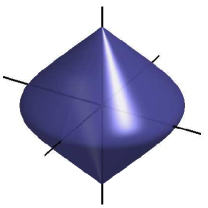
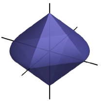
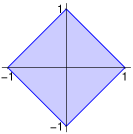
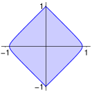
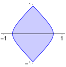
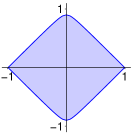
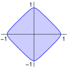
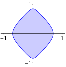
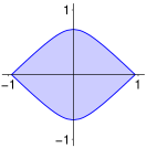
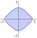
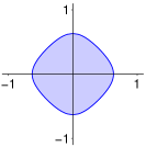
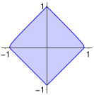
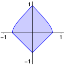
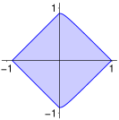
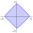
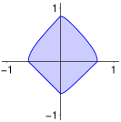
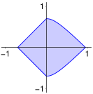
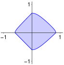
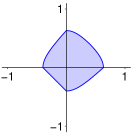
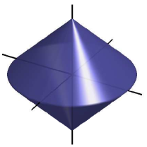
Figures 1 and 2 illustrate the role of each penalty on a problem with $T=2$ tasks and $p=2$ variables. They represent several views of the unit balls

$$\sum_{i=1}^{2}\bigg{(}\sum_{t=1}^{2}{\beta_{i}^{(t)}}^{2}\bigg{)}^{1/2}\leq 1\enspace,\,\text{and}\enspace\\ \sum_{i=1}^{2}\bigg{(}\sum_{t=1}^{2}\left(\beta_{i}^{(t)}\right)_{\!+}^{2}\bigg{)}^{1/2}+\bigg{(}\sum_{t=1}^{2}\left(-\beta_{i}^{(t)}\right)_{\!+}^{2}\bigg{)}^{1/2}\leq 1\enspace,$$

that is, the admissible set for a penalty for a problem with two tasks and two features.

These plots also provide some insight on the sparsity pattern that originate from the penalty, since sparsity is related to the singularities at the boundary of the admissible set (Nikolova 2000). In particular, the first column illustrates that, when $\beta_{2}^{(2)}$ is null, $\beta_{2}^{(1)}$ may also be exactly zero, while the second column shows that this event is improbable when $\beta_{2}^{(2)}$ differs from zero. The second row illustrates the same type of relationship between $\beta_{1}^{(2)}$ and $\beta_{1}^{(1)}$ that are expected due to the symmetries of the unit ball.

	$\beta_{2}^{(2)}=0$	$\beta_{2}^{(2)}=0.1$	$\beta_{2}^{(2)}=0.3$
$\beta_{1}^{(2)}=0$	$\beta_{2}^{(1)}$ $\beta_{1}^{(1)}$	$\beta_{2}^{(1)}$ $\beta_{1}^{(1)}$	$\beta_{2}^{(1)}$ $\beta_{1}^{(1)}$
$\beta_{1}^{(2)}=0.1$	$\beta_{2}^{(1)}$ $\beta_{1}^{(1)}$	$\beta_{2}^{(1)}$ $\beta_{1}^{(1)}$	$\beta_{2}^{(1)}$ $\beta_{1}^{(1)}$
$\beta_{1}^{(2)}=0.3$	$\beta_{2}^{(1)}$ $\beta_{1}^{(1)}$	$\beta_{2}^{(1)}$ $\beta_{1}^{(1)}$	$\beta_{2}^{(1)}$ $\beta_{1}^{(1)}$

Figure 1: Admissible set for the Group-LASSO penalty for a problem with two tasks and two features. Top row: cuts of the unit ball through $(\beta_{1}^{(1)},\beta_{1}^{(2)},\beta_{2}^{(1)})$ for various values of $\beta_{2}^{(2)}$, where $(\beta_{1}^{(1)},\beta_{1}^{(2)})$ span the horizontal plane, and $\beta_{2}^{(1)}$ is on the vertical axis; bottom rows: cuts through $(\beta_{1}^{(1)},\beta_{2}^{(1)})$ for various values of $(\beta_{1}^{(2)}$ and $\beta_{2}^{(2)})$.

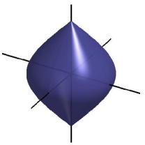
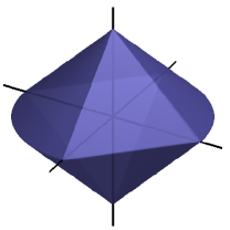
Figure 2 corresponds to a Cooperative-LASSO penalty. These plots should be compared with their Group-LASSO counterpart in Figure 1. We see that there are additional discontinuities in the unit ball resulting in new vertices on the 3-D plots. As before, we have that, when $\beta_{2}^{(2)}$ is null, $\beta_{2}^{(1)}$ may also be exactly zero, but in addition, we may also have $\beta_{1}^{(1)}$ or $\beta_{1}^{(2)}$ exactly null. Accordingly, in the second and third row, we see that we may have $\beta_{2}^{(1)}$ null when $\beta_{2}^{(2)}$ is non-zero. These new edges will result in some new zeroes when the Group-LASSO would have allowed a solution with opposite signs between tasks.

The second main striking difference with Group-LASSO is the loss of the axial symmetry of the Cooperative-LASSO when some variables are non-zero. These plots illustrate that the decoupling of the positive and negative parts of the regression coefficients in the penalty favors solutions where these coefficients are of same sign across tasks. The penalties are identical in the positive and negative orthant, but the Cooperative-LASSO penalization is more stringent elsewhere, when there are some sign mismatches between tasks. The most extreme situation occurs when there is no sign agreement across tasks for all variables. In the setup represented here, with only two tasks, the effective penalty then reduces to the LASSO.

	$\beta_{2}^{(2)}=0$	$\beta_{2}^{(2)}=0.1$	$\beta_{2}^{(2)}=0.3$
$\beta_{1}^{(2)}=0$	$\beta_{2}^{(1)}$ $\beta_{1}^{(1)}$	$\beta_{2}^{(1)}$ $\beta_{1}^{(1)}$	$\beta_{2}^{(1)}$ $\beta_{1}^{(1)}$
$\beta_{1}^{(2)}=0.1$	$\beta_{2}^{(1)}$ $\beta_{1}^{(1)}$	$\beta_{2}^{(1)}$ $\beta_{1}^{(1)}$	$\beta_{2}^{(1)}$ $\beta_{1}^{(1)}$
$\beta_{1}^{(2)}=0.3$	$\beta_{2}^{(1)}$ $\beta_{1}^{(1)}$	$\beta_{2}^{(1)}$ $\beta_{1}^{(1)}$	$\beta_{2}^{(1)}$ $\beta_{1}^{(1)}$

Figure 2: Admissible set for the Cooperative-LASSO penalty for a problem with two tasks and two features. Top row: cuts of the unit ball through $(\beta_{1}^{(1)},\beta_{1}^{(2)},\beta_{2}^{(1)})$ for various values of $\beta_{2}^{(2)}$, where $(\beta_{1}^{(1)},\beta_{1}^{(2)})$ span the horizontal plane, and $\beta_{2}^{(1)}$ is on the vertical axis; bottom rows: cuts through $(\beta_{1}^{(1)},\beta_{2}^{(1)})$ for various values of $(\beta_{1}^{(2)}$ and $\beta_{2}^{(2)})$.

4 Algorithms

In this section, we describe the strategy proposed for solving the three optimization problems introduced above, based upon the proposal of Osborne et al. (2000a) for solving the LASSO. This part also draws its inspiration from Osborne et al. (2000b), Kim et al. (2006), Roth and Fischer (2008).

4.1 Problem Decomposition

The multiple independent tasks Problem (6) can be solved by considering either $T$ single tasks like (4) of size $(p-1)\times p$ (each one possibly decomposed in $p$ LASSO sub-problems of size $p-1$), or a single large problem of size $T\times(p-1)\times p$, which can be decomposed into $p$ LASSO sub-problems of size $(p-1)\times T$, through Proposition 1. This line of attack is not computationally efficient here, but it will become advantageous when considering the penalties presented in Section 3.2. It is introduced at this point to provide a unified conceptual view of all algorithms.

Consider the $(p\,T)\times(p\,T)$ block-diagonal matrix $\mathbf{C}$ composed by the empirical covariance matrices of each tasks

$$\mathbf{C}=\begin{pmatrix}\mathbf{S}^{(1)}&&\text{\Large$0$}\\ &\ddots&\\ \text{\Large 0}&&\mathbf{S}^{(T)}\\ \end{pmatrix},$$

and define

$$\mathbf{C}_{\backslash i\backslash i}=\begin{pmatrix}\mathbf{S}_{\backslash i\backslash i}^{(1)}&&\text{\Large$0$}\\ &\ddots&\\ \text{\Large 0}&&\mathbf{S}_{\backslash i\backslash i}^{(T)}\\ \end{pmatrix},\ \mathbf{C}_{i\backslash i}=\begin{pmatrix}\mathbf{S}_{i\backslash i}^{(1)}\\ \vdots\\ \mathbf{S}_{i\backslash i}^{(T)}\\ \end{pmatrix}.$$ (10)

The $(p-1)\,T\times(p-1)\,T$ matrix $\mathbf{C}_{\backslash i\backslash i}$ is the matrix $\mathbf{C}$ where we removed each line and each column pertaining to variable $i$. We define $\tilde{\mathbf{C}},\tilde{\mathbf{C}}_{\backslash i\backslash i}$ and $\tilde{\mathbf{C}}_{i\backslash i}$ similarly, with $\mathbf{S}^{(t)}$ being replaced by $\tilde{\mathbf{S}}^{(t)}$ for each $t=1,\dots,T$ in the above definitions.

Let ${\boldsymbol{\beta}}^{(t)}\in\mathbb{R}^{(p-1)}$ denote the vector estimating $\mathbf{K}_{i\backslash i}^{(t)}$, defined from $\mathbf{K}^{(t)}$ as in (3), and let $\boldsymbol{\beta}\in\mathbb{R}^{T\times(p-1)}$ be the vector of the concatenated estimates $\boldsymbol{\beta}^{\intercal}=({{\boldsymbol{\beta}}^{(1)}}^{\intercal},\cdots,{{\boldsymbol{\beta}}^{(T)}}^{\intercal})$. The optimization of (6) is achieved by solving $p$ sub-problems in form:

$$\min_{\boldsymbol{\beta}\in\mathbb{R}^{T\times(p-1)}}\frac{1}{2}\left\|\mathbf{C}_{\backslash i\backslash i}^{1/2}\boldsymbol{\beta}+\mathbf{C}_{\backslash i\backslash i}^{-1/2}\mathbf{C}_{i\backslash i}\right\|_{2}^{2}+\lambda\sum_{t=1}^{T}\frac{1}{n_{t}}\left\|\boldsymbol{\beta}\right\|_{1}\enspace.$$ (11)

Note that we do not need to perform the costly matrix operations that are expressed in the the first term of the objective function of Problem (11). In practice, we compute

$$f({\boldsymbol{\beta}};\mathbf{C})=\frac{1}{2}{\boldsymbol{\beta}}^{\intercal}\mathbf{C}_{\backslash i\backslash i}{\boldsymbol{\beta}}+{\boldsymbol{\beta}}^{\intercal}\mathbf{C}_{i\backslash i}\enspace,$$

which only differs from the squared $\ell_{2}$ norm in (11) by a constant that is irrelevant for the optimization process.

Accordingly, Problems (7), (8) and (9) can be decomposed into $p$ minimization sub-problems whose objective functions may be decomposed as

$$L_{k}(\boldsymbol{\beta})=f(\boldsymbol{\beta})+\lambda g_{k}(\boldsymbol{\beta})\enspace,$$ (12)

where, with a slight abuse of notation, $f(\boldsymbol{\beta})$ is either $f({\boldsymbol{\beta}};\tilde{\mathbf{C}})$ for Problem (7) or $f({\boldsymbol{\beta}};\mathbf{C})$ for Problems (8) and (9), and where $g_{k}(\boldsymbol{\beta})$ stands for the penalty functions respectively defined below:

• for the graphical Intertwined LASSO

  $$g_{1}({\boldsymbol{\beta}})=\sum_{t=1}^{T}\frac{1}{n_{t}}\left\|\boldsymbol{\beta}^{(t)}\right\|_{1}\enspace;$$

• for the graphical Group-LASSO

  $$g_{2}({\boldsymbol{\beta}})=\sum_{i=1}^{p-1}\left\|\boldsymbol{\beta}_{i}^{[1:T]}\right\|_{2}\enspace,$$

  where ${\boldsymbol{\beta}_{i}^{[1:T]}}=\left(\beta_{i}^{(1)},\ldots,\beta_{i}^{(T)}\right)^{\intercal}\in\mathbb{R}^{T}$ is the vector of the $i$th component across tasks;

• for the graphical Cooperative-LASSO

  $$g_{3}({\boldsymbol{\beta}})=\sum_{i=1}^{p-1}\left(\left\|\left(\boldsymbol{\beta}_{i}^{[1:T]}\right)_{+}\right\|_{2}+\left\|\left(-\boldsymbol{\beta}_{i}^{[1:T]}\right)_{+}\right\|_{2}\right)\,.$$

Since $f$ is convex with respect to $\boldsymbol{\beta}$, and all penalties are norms, all these objective functions are convex and thus easily amenable to optimization. They are non-differentiable at zero, due to the penalty terms, which all favor zero coefficients. Bearing in mind the typical problems in biological data, where graphs have a few tens or hundreds nodes, and where connectivity is very weak, we need convex optimization tools that are efficient for medium-size problems with extremely sparse solutions. We thus chose a greedy strategy that aims at solving a series of small-size sub-problems, and will offer a simple monitoring of convergence.

4.2 Solving the Sub-Problems

The minimizers $\boldsymbol{\beta}$ of the objective functions (12) are assumed to have many zero coefficients. The approach developed for the LASSO by Osborne et al. (2000a) takes advantage of this sparsity by solving a series of small linear systems, whose size is incrementally increased/decreased, similarly to a column generation algorithm. The master problem is the original problem, but solved only with respect to the subset of variables currently identified as non-zero $\boldsymbol{\beta}$ coefficients. The subproblem of identifying new non-zero variables simply consists in detecting the violations of the first-order optimality conditions with respect to all variables. When there are no more such violations, the current solution is optimal.

The objective functions $L_{k}(\boldsymbol{\beta})$ are convex and smooth except at some locations with zero coefficients. Thus, the minimizer is such that the null vector $\mathbf{0}\in\mathbb{R}^{p-1}$ is an element of the subdifferential $\partial_{\boldsymbol{\beta}}L_{k}(\boldsymbol{\beta})$. In our problems, the subdifferential is given by

$$\partial_{\boldsymbol{\beta}}L_{k}(\boldsymbol{\beta})=\nabla_{\boldsymbol{\beta}}f(\boldsymbol{\beta})+\lambda\partial_{\boldsymbol{\beta}}g_{k}({\boldsymbol{\beta}})\enspace,$$ (13)

where $\nabla_{\boldsymbol{\beta}}f(\boldsymbol{\beta})=\mathbf{C}_{\backslash i\backslash i}\boldsymbol{\beta}+\mathbf{C}_{i\backslash i}$ and where the form of $\partial_{\boldsymbol{\beta}}g_{k}(\boldsymbol{\beta})$ differs for the three problems and will be detailed below.

The algorithm is started from a sparse initial guess, that is, $\boldsymbol{\beta}=\mathbf{0}$ or, if available, the solution obtained on a more constrained problem with a larger penalization parameter $\lambda$. Then, one converges to the global solution iteratively, by managing the index $\mathcal{A}$ of the non-zero coefficients of $\boldsymbol{\beta}$ and solving the master problem over $\mathcal{A}$, where the problem is continuously differentiable. The management of $\mathcal{A}$ requires two steps: the first one removes from $\mathcal{A}$ the coefficients that have been zeroed when solving the previous master problem, ensuring its differentiability at the next iteration, and the second one examines the candidate non-zero coefficients that could enter $\mathcal{A}$. In this process, summarized in Algorithm 1, the size of the bigger master problems is typically of the order of magnitude of the number of non-zero entries in the solution. Solving the master problem with respect to the non-zero coefficients $\boldsymbol{\beta}_{\mathcal{A}}$ can be formalized as solving $\min_{\mathbf{h}}L_{k}(\boldsymbol{\beta}_{\mathcal{A}}+\mathbf{h})$, where $\mathbf{h}\in\mathbb{R}^{|\mathcal{A}|}$ is optimal if $\mathbf{0}\in\partial_{\mathbf{h}}L_{k}(\boldsymbol{\beta}_{\mathcal{A}}+\mathbf{h})$.

// 0. INITIALIZATION

$\boldsymbol{\beta}\leftarrow\mathbf{0}$

$\mathcal{A}\leftarrow\emptyset$

while $\mathbf{0}\notin\partial_{\boldsymbol{\beta}}L(\boldsymbol{\beta})$ do 

// 1. MASTER PROBLEM: OPTIMIZATION WITH RESPECT TO $\boldsymbol{\beta}_{\mathcal{A}}$

Find a (approximate) solution $\mathbf{h}$ to the smooth problem

$$\nabla_{\mathbf{h}}f(\boldsymbol{\beta}_{\mathcal{A}}+\mathbf{h})+\lambda\partial_{\mathbf{h}}g_{k}(\boldsymbol{\beta}_{\mathcal{A}}+\mathbf{h})=0\enspace.$$

// where $\partial_{\mathbf{h}}g_{k}=\left\{\nabla_{\mathbf{h}}g_{k}\right\}$

$\boldsymbol{\beta}_{\mathcal{A}}\leftarrow\boldsymbol{\beta}_{\mathcal{A}}+\mathbf{h}$

// 2. IDENTIFY NEWLY ZEROED VARIABLES

while $\exists i\in\mathcal{A}:\beta_{i}=0$ and ${\displaystyle\min_{\theta\in\partial_{\beta_{i}}g_{k}}}\left|\frac{\partial f(\boldsymbol{\beta})}{\partial\beta_{i}}+\lambda\theta\right|=0$ do  $\mathcal{A}\leftarrow\mathcal{A}\backslash\{i\}$

 

// 3. IDENTIFY NEW NON-ZERO VARIABLES

// Select $i\in\mathcal{A}^{c}$ such that an infinitesimal change of $\beta_{i}$ provides the highest reduction of $L_{k}$

${\displaystyle i\leftarrow\mathop{\mathrm{arg\ max}}_{j\in\mathcal{A}^{c}}v_{j}}$, where ${\displaystyle v_{j}=\min_{\theta\in\partial_{\beta_{j}}g_{k}}}\left|\frac{\partial f(\boldsymbol{\beta})}{\partial\beta_{j}}+\lambda\theta\right|$

if $v_{i}\neq 0$ then  $\mathcal{A}\leftarrow\mathcal{A}\cup\left\{i\right\}$

else  Stop and return $\boldsymbol{\beta}$, which is optimal

   

Algorithm 1 General optimization algorithm

4.3 Implementation Details

We provide below the implementation details that are specific to each optimization problem. Specificity of each problem relies on $\partial_{\boldsymbol{\beta}}g_{k}({\boldsymbol{\beta}})$, denoted ${\boldsymbol{\theta}}$ herein.

Intertwined LASSO –

This LASSO problem is solved as proposed by Osborne et al. (2000a), except that we consider here the Lagrangian formulation with $\lambda$ fixed.

The components of $\boldsymbol{\theta}$ in the subdifferential (13) read

$$\text{if}\enspace\beta_{i}=0\enspace\text{then}\enspace\theta_{i}\in[-1,1]\enspace\enspace,\ \text{else}\enspace\theta_{i}=\mathrm{sign}({\beta}_{i})\enspace.$$

Solving the master problem on $\mathcal{A}$ requires an estimate of $\boldsymbol{\theta}_{\mathcal{A}}$ at $\boldsymbol{\beta}_{\mathcal{A}}+\mathbf{h}$ . It is computed based on a local approximation, where the components of $\mathrm{sign}(\boldsymbol{\beta}_{\mathcal{A}}+\mathbf{h})$ are replaced by $\mathrm{sign}(\boldsymbol{\beta}_{\mathcal{A}})$.  This leads to the following descent direction $\mathbf{h}$:

$$\mathbf{h}=-\boldsymbol{\beta}_{\mathcal{A}}-\tilde{\mathbf{C}}_{\backslash i\backslash i}^{-1}(\mathcal{A},\mathcal{A})(\tilde{\mathbf{C}}_{i\backslash i}(\mathcal{A})+\lambda\boldsymbol{\theta}_{\mathcal{A}})\enspace,$$

where, in order to avoid double subscripts, we use the notation $\mathbf{M}(\mathcal{A},\mathcal{A})$ for the square submatrix of $\mathbf{M}$ formed by the rows and columns indexed by $\mathcal{A}$, and $\mathbf{v}(\mathcal{A})$ for the subvector formed by the columns of $\mathbf{v}$ indexed by $\mathcal{A}$.

Then, before updating $\boldsymbol{\beta}_{\mathcal{A}}$, one checks whether the local approximation used to compute $\mathbf{h}$ is consistent with the sign of the new solution. If not the case, one looks for the largest step size $\rho$ in direction $\mathbf{h}$ such that $\boldsymbol{\beta}_{\mathcal{A}}^{+}=\boldsymbol{\beta}_{\mathcal{A}}+\rho\mathbf{h}$ is sign-consistent with $\boldsymbol{\beta}_{\mathcal{A}}$. This amounts to zero a coefficient, say $\beta_{i}$, and $i$ is removed from $\mathcal{A}$ if $|\partial f(\boldsymbol{\beta}^{+})/\partial\beta_{i}|<\lambda$ , otherwise, the corresponding $\theta_{i}$ is set to $-\mathrm{sign}(\partial f(\boldsymbol{\beta}^{+})/\partial\beta_{i})$ . In any case, a new direction $\mathbf{h}$ is computed as above, and $\boldsymbol{\beta}_{\mathcal{A}}$ is updated until the optimality conditions are reached within $\mathcal{A}$.

Finally, the global optimum is attained if the first-order optimality conditions are met for all the components of $\boldsymbol{\beta}$, that is, if $\widehat{\boldsymbol{\beta}}$ verifies

$$\mathbf{0}\in\widetilde{\mathbf{C}}_{\backslash i\backslash i}\widehat{\boldsymbol{\beta}}+\widetilde{\mathbf{C}}_{i\backslash i}+\lambda\boldsymbol{\theta}\enspace,$$

where ${\boldsymbol{\theta}}$ is such

$$\boldsymbol{\theta}_{\mathcal{A}}=\mathrm{sign}(\widehat{\boldsymbol{\beta}}_{\mathcal{A}})\quad\text{and}\quad\left\|\boldsymbol{\theta}_{\mathcal{A}^{c}}\right\|_{\infty}\leq 1\enspace.$$

Graphical Group-LASSO –

In this problem, the subdifferential (13) is conditioned on the norm of $\boldsymbol{\beta}_{i}^{[1:T]}$, the vector of the $i$th component across tasks. Let $\boldsymbol{\theta}_{i}^{[1:T]}=\left(\theta_{i}^{(1)},\ldots,\theta_{i}^{(T)}\right)^{\intercal}\in\mathbb{R}^{T}$ be defined similarly to $\boldsymbol{\beta}_{i}^{[1:T]}$, we have that,

$$\text{if}\enspace\left\|\boldsymbol{\beta}_{i}^{[1:T]}\right\|_{2}=0\enspace\text{then}\enspace\left\|\boldsymbol{\theta}_{i}^{[1:T]}\right\|_{2}\leq 1\enspace\enspace,\ \\ \text{else}\enspace\boldsymbol{\theta}_{i}^{[1:T]}=\left\|\boldsymbol{\beta}_{i}^{[1:T]}\right\|_{2}^{-1}\boldsymbol{\beta}_{i}^{[1:T]}\enspace,$$

where, here and in what follows, $0/0$ is defined by continuation as $0/0=0$. As the subgradient w.r.t. $\boldsymbol{\beta}_{i}^{[1:T]}$ reduces to a gradient whenever one component of $\boldsymbol{\beta}_{i}^{[1:T]}$ is non-zero, the management of the null variables is done here by subsets of $T$ variables, according to $\left\|\nabla_{\boldsymbol{\beta}_{i}^{[1:T]}}f(\boldsymbol{\beta})\right\|_{2}$, instead of the one by one basis of the LASSO. Hence, we only need to index the groups $i\in\{1,\ldots,p-1\}$ in $\mathcal{A}$.

Here also, solving the master problem on $\mathcal{A}$ requires an estimate of $\boldsymbol{\theta}_{\mathcal{A}}^{[1:T]}$ at $\boldsymbol{\beta}_{\mathcal{A}}^{[1:T]}+\mathbf{h}$ . Provided that $\left\|\boldsymbol{\beta}_{i}^{[1:T]}\right\|_{2}\neq 0$ for all $i\in\mathcal{A}$, $\boldsymbol{\theta}_{\mathcal{A}}^{[1:T]}$ is differentiable w.r.t. $\boldsymbol{\beta}_{\mathcal{A}}^{[1:T]}$. It will thus be approximated by a first-order Taylor expansion, resulting in a Newton-Raphson or quasi-Newton step. Here, we used quasi-Newton with BFGS updates. Note that, whenever $\boldsymbol{\beta}_{i}^{[1:T]}=\mathbf{0}$, that is, when a new group of variables has just been activated or is about to be deactivated, the corresponding $\boldsymbol{\theta}_{i}^{[1:T]}$ is set so that

$$\left\|\nabla_{\boldsymbol{\beta}_{i}^{[1:T]}}f(\boldsymbol{\beta})+\lambda\boldsymbol{\theta}_{i}^{[1:T]}\right\|_{2}$$ (14)

is minimum (that is, with $\boldsymbol{\theta}_{i}^{[1:T]}$ proportional to $\nabla_{\boldsymbol{\beta}_{i}^{[1:T]}}f$). The updates of $\mathcal{A}$ are also based on the minimal value of (14).

Graphical Cooperative-LASSO –

As the Group-LASSO, the Cooperative-LASSO considers a group structure, but its implementation differs considerably from the former in the management of $\mathcal{A}$. Though several variables are usually activated or deactivated at the same time, they typically correspond to subsets of $\boldsymbol{\beta}_{i}^{[1:T]}$, and these subsets are context-dependent; they are not defined beforehand. As a result, the index of non-zero $\boldsymbol{\beta}_{i}^{[1:T]}$ is better handled by considering two sets: the index of $\boldsymbol{\beta}_{i}^{[1:T]}$ with positive and negative components:

$$\begin{array}[]{rl@{\hfill}}&\mathcal{A}_{+}=\left\{i\in\left\{1,\ldots,p-1\right\}:\left\|\left(\boldsymbol{\beta}_{i}^{[1:T]}\right)_{+}\right\|_{2}>0\right\}\enspace,\\[10.76385pt] \text{and}&\mathcal{A}_{-}=\left\{i\in\left\{1,\ldots,p-1\right\}:\left\|\left(-\boldsymbol{\beta}_{i}^{[1:T]}\right)_{+}\right\|_{2}>0\right\}\enspace.\end{array}$$

Let $\mathcal{T}$ denote the index of non-zero entries of $\boldsymbol{\beta}_{i}^{[1:T]}$, with complement $\mathcal{T}^{c}$; the subdifferential at the current solution is such that:

• if $i\in\mathcal{A}_{+}^{c}\cap\mathcal{A}_{-}^{c}$, then

  $$\max\left(\left\|\left(\boldsymbol{\theta}_{i}^{[1:T]}\right)_{+}\right\|_{2},\left\|\left(-\boldsymbol{\theta}_{i}^{[1:T]}\right)_{+}\right\|_{2}\right)\leq 1\,;$$

• if $i\in\mathcal{A}_{+}^{c}\cap\mathcal{A}_{-}$ then

  $$\boldsymbol{\theta}_{i}^{\mathcal{T}}=\left\|\left(-\boldsymbol{\beta}_{i}^{\mathcal{T}}\right)_{+}\right\|_{2}^{-1}\boldsymbol{\beta}_{i}^{\mathcal{T}}\,,$$

  $$\boldsymbol{\theta}_{i}^{\mathcal{T}^{c}}:\left\|\left(\boldsymbol{\theta}_{i}^{\mathcal{T}^{c}}\right)_{+}\right\|_{2}\leq 1\ \text{and}\ \left\|\left(-\boldsymbol{\theta}_{i}^{\mathcal{T}^{c}}\right)_{+}\right\|_{2}=0\,;$$

• $i\in\mathcal{A}_{+}\cap\mathcal{A}_{-}^{c}$, then

  $$\boldsymbol{\theta}_{i}^{\mathcal{T}}=\left\|\left(\boldsymbol{\beta}_{i}^{\mathcal{T}}\right)_{+}\right\|_{2}^{-1}\boldsymbol{\beta}_{i}^{\mathcal{T}}\,,$$

  $$\boldsymbol{\theta}_{i}^{\mathcal{T}^{c}}:\left\|\left(-\boldsymbol{\theta}_{i}^{\mathcal{T}^{c}}\right)_{+}\right\|_{2}\leq 1\ \text{and}\ \left\|\left(\boldsymbol{\theta}_{i}^{\mathcal{T}^{c}}\right)_{+}\right\|_{2}=0\,;$$

• if $i\in\mathcal{A}_{+}\cap\mathcal{A}_{-}$, then

  $$\theta_{i}^{(t)}=\left\|\left(\mathrm{sign}\big{(}{\beta}_{i}^{(t)}\big{)}\boldsymbol{\beta}_{i}^{[1:T]}\right)_{+}\right\|_{2}^{-1}\beta_{i}^{(t)}\enspace,\ t=1,\ldots,T\,.$$

Once $\mathcal{A}^{+}$ and $\mathcal{A}^{-}$ are determined, the master problem is solved as for the Group-LASSO, with BFGS updates, with box constraints to ensure sign feasible $\boldsymbol{\beta}_{i}^{[1:T]}$ for $i$ such that $i\in\mathcal{A}_{+}^{c}\cap\mathcal{A}_{-}$ or $i\in\mathcal{A}_{+}\cap\mathcal{A}_{-}^{c}$. When a new variable has just been activated or is about to be deactivated, the corresponding $\boldsymbol{\theta}_{i}^{[1:T]}$ is set so that

$$\left\|\left(\nabla_{\boldsymbol{\beta}_{i}^{[1:T]}}f(\boldsymbol{\beta})+\lambda\boldsymbol{\theta}_{i}^{[1:T]}\right)_{+}\right\|_{2}\\ +\left\|\left(-\nabla_{\boldsymbol{\beta}_{i}^{[1:T]}}f(\boldsymbol{\beta})-\lambda\boldsymbol{\theta}_{i}^{[1:T]}\right)_{+}\right\|_{2}$$ (15)

is minimum. The updates of $\mathcal{A}$ are also based on the minimal value of (15).

5 Experiments

In most real-life applications, the major part of the inferred graphs are unknown, with little available information on the presence/absence of edges. We essentially face an unsupervised learning problem, where there is no objective criterion allowing to compare different solutions. As a result, setting the hyper-parameters is particularly troublesome, alike, say, choosing the number of components in a mixture model, and it is a common practice to visualize several networks corresponding to a series of penalties.

Regarding the first issue, we chose to present here synthetic and well-known real data that allow for an objective quantitative evaluation. Regarding the second issue, the problem of choosing penalty parameters can be guided by theoretical results that provide a bound on the rate of false edge discovery (Meinshausen and Bühlmann 2006, Banerjee et al. 2008, Ambroise et al. 2009), or by more traditional information criteria targeting the estimation of $\mathbf{K}$ (Yuan and Lin 2007, Rocha et al. 2008). However, these proposals tend to behave poorly, and it is a usual practice to compare the performance of learning algorithms by providing a series of results, such as precision-recall plots or ROC-curves, letting the choice of penalty parameters as a mostly open question for future research. Although the shortcomings of this type of comparison are well-known (Drummond and Holte 2006, Bengio et al. 2005), we will use precision vs. recall plots, which can be considered as valuable exploratory tools.

Precision is the ratio of the number of true selected edges to the total number of selected edges in the inferred graphs. Recall is the ratio of the number of true selected edges in the inferred graphs to the total number of edges in the true graphs. In a statistical framework, the recall is equivalent to the power and the precision is equivalent to one minus the false discovery proportion.

5.1 Synthetic Data

5.1.1 Simulation Protocol

To generate $T$ samples stemming from a similar graph, we first draw an “ancestor” graph with $p$ nodes and $k$ edges according to the Erdős-Rényi model. Here, we consider a simple setting with $T=4$ and a network with $p=20$ nodes and $k=20$ edges, as illustrated in Figure 3.

Figure 3: Set of simulated graphs: ancestor (top) and two children (bottom) engendered by a $\delta=2$ perturbation.

Then, $T$ children graphs are produced by random addition and deletion of $\delta$ edges in the ancestor graph. The $T$ concentration matrices are built from the normalized graph Laplacians, whose off-diagonal elements are slightly deflated to produce strictly diagonally dominant matrices. To allow for positively and negatively correlated variables, we generate a strictly triangular matrix of random signs drawn from a Rademacher distribution. This matrix is symmetrized, complemented with ones on the diagonal, and its component-wise multiplication with the deflated Laplacians produces the ground-truth for the concentration matrices $\mathbf{K}^{(1)},\dots,\mathbf{K}^{(T)}$. Each $\mathbf{K}^{(t)}$ is finally used to generate $n$ Gaussian vectors with zero mean and covariance ${\mathbf{K}^{(t)}}^{-1}$.

5.1.2 Experimental Setup

The precision-recall plots are computed by considering the cumulative number of true and false edge detections among the $T=4$ children networks. Let ${\cal E}^{(t)}$ be the set of edges for children network $t$, precision and recall are respectively formaly defined as:

$$\frac{\displaystyle\sum_{t=1}^{T}\sum_{(i,j)\in{\cal E}^{(t)}}\mathbf{1}(\widehat{K}_{ij}^{(t)})}{\displaystyle\sum_{t=1}^{T}\sum_{i>j}\mathbf{1}(\widehat{K}_{ij}^{(t)})}\enspace\mbox{and}\enspace\frac{\displaystyle\sum_{t=1}^{T}\sum_{(i,j)\in{\cal E}^{(t)}}\mathbf{1}(\widehat{K}_{ij}^{(t)})}{\displaystyle\sum_{t=1}^{T}\left|{\cal E}^{(t)}\right|}\enspace,$$

where $\widehat{K}_{ij}^{(t)}$ is the estimated partial correlation between variables $i$ and $j$ for network $t$, $\mathbf{1}(u)$ returns $1$ if $u\neq 0$ and $0$ otherwise, and $\left|{\cal E}\right|$ is the cardinal of ${\cal E}$.

To ensure representativeness, the precision-recall figures are averaged over 100 random draws of the ancestor graph, the averaging being performed for fixed values of the penalization parameter $\lambda$. That is, each point in the (precision,recall) plane is the average of the 100 points obtained for each random draw of the ancestor graph, for a given estimation method and for a given value of the penalization parameter. We compare our proposals, namely the Graphical Intertwined ($\alpha=1/2$), Cooperative and Group LASSO to two baselines: the original neighborhood selection of Meinshausen and Bühlmann (2006), either applied separately to each graph (annotated “independent”), or computed on the data set merging the data originating from all graphs (annotated “pooled”).

5.1.3 Results

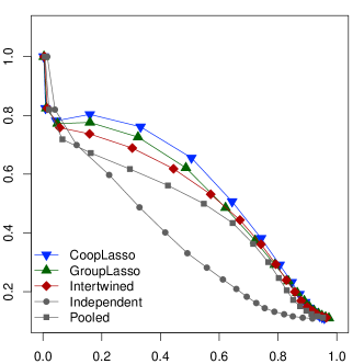
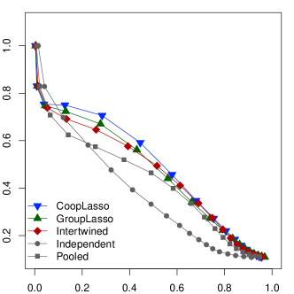
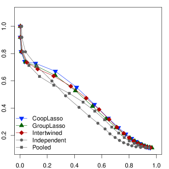
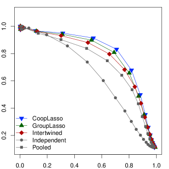
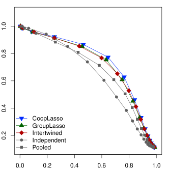
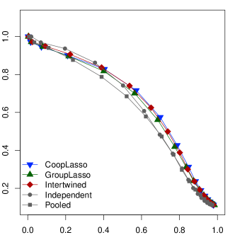
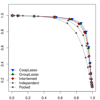
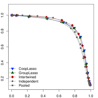
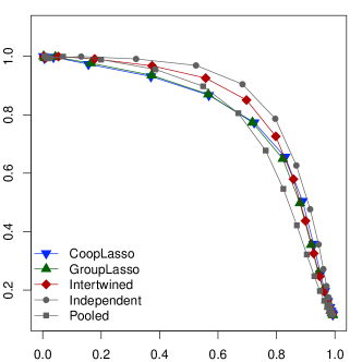
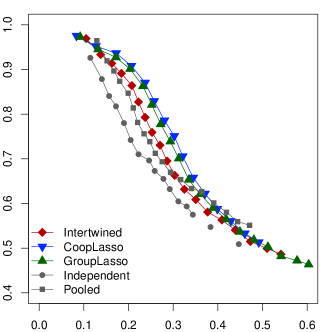
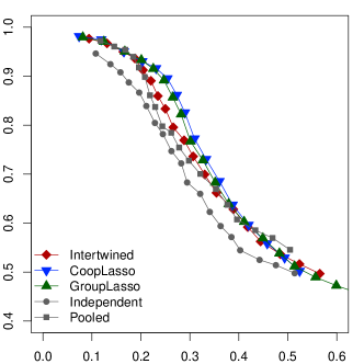
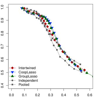
Figures 4, 5 and 6 display precision-recall plots for nine prototypical situations.

$\delta=1$	Precision
		Recall
$\delta=3$	Precision
		Recall
$\delta=5$	Precision
		Recall

Figure 4: Precision-recall curves for the Intertwined, Cooperative, Group and the two baseline LASSO, for inferring four graphs (each with $p=20$ nodes, $k=20$ edges and a perturbation $\delta$ from the ancestor graph) from four samples of size $n_{t}=25$.

$\delta=1$	Precision
		Recall
$\delta=3$	Precision
		Recall
$\delta=5$	Precision
		Recall

Figure 5: Precision-recall curves for the Intertwined, Cooperative, Group and the two baseline LASSO, for inferring four graphs (each with $p=20$ nodes, $k=20$ edges and a perturbation $\delta$ from the ancestor graph) from four samples of size $n_{t}=50$.

$\delta=1$	Precision
		Recall
$\delta=3$	Precision
		Recall
$\delta=5$	Precision
		Recall

Figure 6: Precision-recall curves for the Intertwined, Cooperative, Group and the two baseline LASSO, for inferring four graphs (each with $p=20$ nodes, $k=20$ edges and a perturbation $\delta$ from the ancestor graph) from four samples of size $n_{t}=100$.

From Figure 4 to 6, the sample size increases, and from top to bottom, the differentiation between networks increases. First, note that the independent strategy is not influenced by the level of perturbation, yet only by the sub-sample size, as expected.

The top graph in Figure 4 represents the small-sample low-perturbation situation, where merging data sets is a good strategy, leveraging the independent analysis. The latter performs poorly, and our multi-task approaches dominate the pooled strategy, the Cooperative-LASSO being superior to the Group-LASSO, which has the advantage on the Intertwined LASSO. The medium/large-sized-sample low-perturbation (top graph in Figures 5 and 6), small/medium-sized-sample medium-perturbation (middle graph in Figures 4 and 5) and small-sized-sample large-perturbation (bottom graph in Figure 4) are qualitatively similar, with less differences between all competitors. For the large-sample medium-perturbation (middle graph in Figure 6) and medium-sized-sample low-perturbation (bottom graph in Figure 5) cases, all methods perform similarly. There is a slight advantage for the multi-task strategies for high recalls, and a slight advantage for the independent analysis for low recalls (that is, for high penalization, where there is less effective degrees of freedom to determine). The bottom graph in Figure 6 represents the large-sample high-perturbation situation, where merging data is a bad strategy, since the networks differ significantly and there is enough data to estimate each network independently. The independent strategy works best, closely followed by the Intertwined LASSO. The Cooperative and Group-LASSO behave equally well for high recalls (low penalization parameters), but for highly penalized solutions (low recalls), they eventually become slightly worse than the pooled estimation.

These experiments show that our proposals are valuable, especially in the most common situation where data are scarce. Among the baselines, the usual pooled sample strategy is good in the small-sample low-perturbation, and the opposite independent strategy is better in the large-sample high-perturbation case. The intertwined LASSO is very robust, in the sense that it always performs favorably compared to the best baseline method over the whole spectrum of situations. Furthermore, except for the large-sample high-perturbation case, the Group-LASSO performs even better, and the Cooperative-LASSO improves further the supremacy of the multiple graph inference approach.

5.2 Protein Signaling Network

Only a few real data sets come with a reliable and exhaustive ground-truth allowing quantitative assessments. We make use of a multivariate flow cytometry data set pertaining to a well-studied human T-cell signaling pathway (Sachs et al. 2005). The latter involves 11 signaling molecules (phospholipids and phosphorylated proteins) and 20 interactions described in the literature. The signaling network is perturbed by activating or inhibiting the production of a given molecule. Fourteen assays have been conducted, aiming to reveal different part of the network. Here, we used only four assays (inhibition of PKC, activation of PKC, inhibition of AKT, activation of PKA).

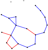
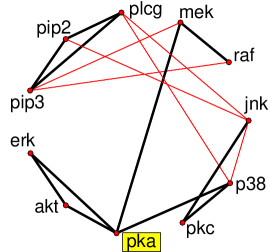
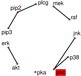
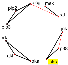
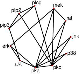
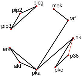
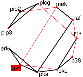
Graphs inferred using only one assay at a time show that each assay really focus on different part of the network (see Figure 7).

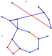
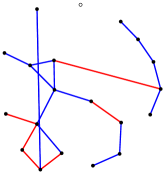
Figure 7: Four graphs inferred from single assay. From left to right, top to bottom, we have respectively graphs inferred from an assay: inhibiting akt, activating pka, inhibiting pkc, activating pkc. Thick black lines represent true positive and thin red lines are false positive.

Figure 8: Ground-truth pathway (left) and graph sum of the four graphs estimated by Intertwined LASSO using all data (right). Thick black lines represent true positive and thin red lines are false positive.

When considering a strategy based on inference from multiple assays, the first false positive inferred by the Intertwined Graphical LASSO occurs when 11 true interactions out of 20 are detected (see Figure 8). This edge, between p38 and Jnk, is in fact due to an indirect connection via unmeasured MAP kinase kinases (Sachs et al. 2005), which is a typical problem of confounding arising in this context. Considering partial correlations within the subset of available variables, the edge is correctly detected, but it is a false positive with respect to the biological ground truth. Furthermore, in larger biological networks, the absence of edge in the ground truth pathway often merely means that there is yet no evidence that the co-regulation exists. As a result, most real data evaluation of graph inference methods are based on qualitative subjective assessments by experts.

This caveat being, the various inference algorithms behave here as in the synthetic experiments: all inference methods perform about equally well for large samples (each assay consists here of about 1000 repeated measurements).

$n_{t}=7$	Precision
		Recall
$n_{t}=10$	Precision
		Recall
$n_{t}=20$	Precision
		Recall

Figure 9: Precision-recall curves for the Intertwined, Cooperative, Group and the two baseline LASSO, for inferring the graphs on four assays of Sachs’ data from four samples of size $n_{t}=7,10$ and $20$.

Figure 9 displays the results obtained for small sample sizes. Here also, the precision-recall plots are averaged over 100 independent random draws of samples of size $n_{t}$, that is $n=4n_{t}$ observations over the four considered assays. It is worth noticing that the large sample size limit is almost obtained for $n_{t}=20$. As for the synthetic experiments, the averaging is performed for fixed values of the penalization parameter $\lambda$. In this situation, our proposals dominate the best baseline strategy, which is pooled estimation. Again, the Intertwined LASSO is very robust, but the Group-LASSO, and to a greater extent the Cooperative-LASSO perform better in the small-sample-size regime.

6 Conclusion

This paper presents the first methods dedicated to the inference of multiple graphs in the Gaussian Graphical Model framework. In this setup, the two baseline approaches consist in either handling the inference problems separately or as a single one by merging the available data sets. Our proposals, motivated by bioinformatics applications, were devised to describe the dependencies between pairs of variables in analogous operating conditions, such as measurements recorded in different assays. This situation occurs routinely with omics data.

Our approaches are based on the neighborhood selection of Meinshausen and Bühlmann (2006). The first one, the Intertwined Graphical LASSO, relaxes the uniqueness constraint that is implicit when the tasks are processed as a single one, merely biasing the results towards a common answer. Our second approach, the Graphical Cooperative-LASSO, is based on a group-penalty that favors similar graphs, with homogeneous dependencies between the same pairs of variables. Homogeneity is quantified here by the magnitude and sign of partial correlations. The Cooperative-LASSO contrasts the Group-LASSO in being able to infer differing graph structures across tasks. Our experimental results show that our proposals are valuable and robust, consistently performing at least as well as the best of the two baseline solutions.

The algorithms developed in this paper are made available within the R-package simone from version 1.0-0 and later. This package also embeds extension of the multi-task framework to time-course data, that is, when transcriptomics data are collected by considering the same individual across time. This implementation builds on the $\ell_{1}$-penalized VAR(1) model described in Charbonnier et al. (2010).

As future work, we will provide a theoretical analysis of the Cooperative-LASSO regarding uniqueness of the solution and selection consistency, or sparsistence, that corresponds here to the asymptotic convergence of the set of detected edges towards the set of true edges.

Appendix A Proofs

A.1 Derivation of the pseudo-log-likelihood

We show here that the pseudo-log-likelihood

$$\mathcal{L}(\mathbf{K}|\mathbf{X})=\sum_{i=1}^{p}\left(\sum_{k=1}^{n}\log\mathbb{P}(X_{i}^{k}|X^{k}_{\backslash i};\mathbf{K}_{i})\right)\enspace,$$ (16)

associated to a sample of size $n$ drawn independently from the multivariate Gaussian vector $X\sim\mathcal{N}(\mathbf{0}_{p},{\boldsymbol{\Sigma}})$ reads

$$\mathcal{L}(\mathbf{K}|\mathbf{X})=\frac{n}{2}\log\det(\mathbf{D})-\frac{n}{2}\mathrm{Tr}\left(\mathbf{D}^{-\frac{1}{2}}\mathbf{K}\mathbf{S}\mathbf{K}\mathbf{D}^{-\frac{1}{2}}\right)-\frac{np}{2}\log(2\pi)\enspace,$$

where $\mathbf{S}=n^{-1}\mathbf{X}^{\intercal}\mathbf{X}$ is the empirical variance-covariance matrix and $\mathbf{D}$ is the diagonal matrix such that $D_{ii}=K_{ii}$, for $i=1,\dots,p$.

Proof.

Since the joint distribution of $X^{k}$ is Gaussian, the distributions of $X_{i}^{k}$ conditioned on the remaining variables $X_{\backslash i}^{k}$ are also Gaussian. Their parameters $(\mu_{i}^{k},\sigma_{i})$ are given by

$$\mu_{i}^{k}={\boldsymbol{\Sigma}}_{i\backslash i}^{\intercal}{\boldsymbol{\Sigma}}^{-1}_{\backslash i\backslash i}X_{\backslash i}^{k}\enspace,\qquad\sigma_{i}={\Sigma}_{ii}-{\boldsymbol{\Sigma}}_{i\backslash i}^{\intercal}{\boldsymbol{\Sigma}}^{-1}_{\backslash i\backslash i}{\boldsymbol{\Sigma}}_{i\backslash i}\enspace.$$ (17)

where ${\boldsymbol{\Sigma}}_{\backslash i\backslash i}$ is matrix ${\boldsymbol{\Sigma}}$ deprived of its $i$th column and its $i$th line, ${\boldsymbol{\Sigma}}_{i\backslash i}$ is the $i$th column of matrix ${\boldsymbol{\Sigma}}$ deprived of its $i$th element.

As $\mathbf{K}=\mathbf{{\boldsymbol{\Sigma}}}^{-1}$, reordering the rows and columns of the matrices yields

$$\begin{bmatrix}{\boldsymbol{\Sigma}}_{\backslash i\backslash i}&{\boldsymbol{\Sigma}}_{i\backslash i}\\ {\boldsymbol{\Sigma}}_{i\backslash i}^{\intercal}&{\Sigma}_{ii}\\ \end{bmatrix}\times\begin{bmatrix}\mathbf{K}_{\backslash i\backslash i}&\mathbf{K}_{i\backslash i}\\ \mathbf{K}_{i\backslash i}^{\intercal}&K_{ii}\\ \end{bmatrix}=\begin{bmatrix}I_{p-1}&0\\ 0&1\\ \end{bmatrix},$$

where $\mathbf{K}_{\backslash i\backslash i}$ is matrix $\mathbf{K}$ deprived of its $i$th column and its $i$th line, $\mathbf{K}_{i\backslash i}$ is the $i$th column of matrix $\mathbf{K}$ deprived of its $i$th element, and $I_{p-1}$ is the identity matrix of size $p-1$. Two of these blockwise equalities are rewritten as follows:

$$\Sigma_{ii}=(1-{\boldsymbol{\Sigma}}_{i\backslash i}^{\intercal}\mathbf{K}_{i\backslash i})/K_{ii}\enspace,$$

$${\boldsymbol{\Sigma}}_{\backslash i\backslash i}^{-1}{\boldsymbol{\Sigma}}_{i\backslash i}=-\mathbf{K}_{i\backslash i}/K_{ii}\enspace.$$

Using the above identities in (17), we obtain

$$\sigma_{i}=(1-{\boldsymbol{\Sigma}}_{i\backslash i}^{\intercal}\mathbf{K}_{i\backslash i})/K_{ii}+{\boldsymbol{\Sigma}}_{i\backslash i}^{\intercal}\mathbf{K}_{i\backslash i}/K_{ii}=1/K_{ii}\enspace,$$

$${\boldsymbol{\mu}}_{i}=-\mathbf{K}_{i\backslash i}^{\intercal}{\mathbf{X}}_{\backslash i}^{\intercal}/K_{ii}.$$

where ${\boldsymbol{\mu}}_{i}=(\mu_{i}^{1},\dots,\mu_{i}^{n})^{\intercal}$.

Using these notations and the corresponding blockwise notations for $\mathbf{S}$ ($S_{ii}=n^{-1}{\mathbf{X}}_{i}^{\intercal}{\mathbf{X}}_{i}$, $\mathbf{S}_{i\backslash i}=n^{-1}{\mathbf{X}}_{\backslash i}^{\intercal}{\mathbf{X}}_{i}$ and $\mathbf{S}_{\backslash i\backslash i}=n^{-1}{\mathbf{X}}_{\backslash i}^{\intercal}{\mathbf{X}}_{\backslash i}$), Equation (16) reads

$$\mathcal{L}(\mathbf{K}|{\mathbf{X}}) =-\frac{n}{2}\sum_{i=1}^{p}\log\sigma_{i}-\sum_{i=1}^{p}\frac{1}{2\sigma_{i}}({\mathbf{X}}_{i}-{\boldsymbol{\mu}}_{i})^{\intercal}({\mathbf{X}}_{i}-{\boldsymbol{\mu}}_{i})-\frac{np}{2}\log(2\pi)$$

$$=\ \frac{n}{2}\sum_{i=1}^{p}\log K_{ii}-\frac{np}{2}\log(2\pi)$$

$$\hskip 30.00005pt-\frac{n}{2}\sum_{i=1}^{p}K_{ii}\left(S_{ii}+\frac{2}{K_{ii}}\mathbf{S}_{i\backslash i}^{\intercal}\mathbf{K}_{i\backslash i}+\frac{1}{K_{ii}^{2}}\mathbf{K}_{i\backslash i}^{\intercal}\mathbf{S}_{\backslash i\backslash i}\mathbf{K}_{i\backslash i}\right)$$ (18)

$$=\ \frac{n}{2}\log\det\mathbf{D}-\frac{np}{2}\log(2\pi)-\frac{n}{2}\sum_{i=1}^{p}\frac{1}{K_{ii}}\left(\mathbf{K}_{i}^{\intercal}\mathbf{S}\mathbf{K}_{i}\right),$$

where $\mathbf{K}_{i}$ is the $i$th column of $\mathbf{K}$ and $\mathbf{D}$ is the diagonal matrix such that $D_{ii}=K_{ii}$. Finally, we use that $\sum_{i=1}^{p}\frac{1}{K_{ii}}\left(\mathbf{K}_{i}^{\intercal}\mathbf{S}\mathbf{K}_{i}\right)=\mathrm{Tr}(\mathbf{D}^{-\frac{1}{2}}\mathbf{K}\mathbf{S}\mathbf{K}\mathbf{D}^{-\frac{1}{2}})$ to conclude the proof. ∎

A.2 Blockwise Optimization of the pseudo-log-likelihood

Proof of Proposition 1.

From (18), we have

$$\mathcal{L}(\mathbf{K}|\mathbf{S})=-\frac{n}{2}\sum_{i=1}^{p}\left(2\mathbf{S}_{i\backslash i}^{\intercal}\mathbf{K}_{i\backslash i}+\frac{1}{K_{ii}}\mathbf{K}_{i\backslash i}^{\intercal}\mathbf{S}_{\backslash i\backslash i}\mathbf{K}_{i\backslash i}\right)+c,$$ (19)

where $c$ does not depend on $K_{ij}$ with $j\neq i$. Thus, if we discard the symmetry constraint on $\mathbf{K}$, maximizing the pseudo-likelihood (19) with respect to the non-diagonal entries of $\mathbf{K}$ amounts to solve $p$ independent maximization problems with respect to $\mathbf{K}_{i\backslash i}$ , $i=1,\ldots,p$. The summands of (19) can be rewritten as

$$-\frac{n}{2K_{ii}}\left(2K_{ii}\mathbf{S}_{i\backslash i}^{\intercal}\mathbf{K}_{i\backslash i}+\mathbf{K}_{i\backslash i}^{\intercal}\mathbf{S}_{\backslash i\backslash i}\mathbf{K}_{i\backslash i}\right)\\ =-\frac{nK_{ii}}{2}\left\|K_{ii}^{-1}\mathbf{S}_{\backslash i\backslash i}^{1/2}\mathbf{K}_{i\backslash i}+\mathbf{S}_{\backslash i\backslash i}^{-1/2}\mathbf{S}_{i\backslash i}\right\|_{2}^{2}+c^{\prime},$$

where $c^{\prime}={n}/{2}\,K_{ii}\mathbf{S}_{i\backslash i}^{\intercal}\mathbf{S}_{\backslash i\backslash i}\mathbf{S}_{i\backslash i}$ does not depend on $K_{ij}$ with $j\neq i$. Adding an $\ell_{1}$ penalty term on $\mathbf{K}_{i\backslash i}$ and defining $\boldsymbol{\beta}=K_{ii}^{-1}\mathbf{K}_{i\backslash i}$ leads to the objective function of Problem (5), which concludes the proof. ∎

A.3 Subdifferential for the Cooperative-LASSO

By definition, for a convex function $g$, the subdifferential is

$$\left.\partial g\right|_{\boldsymbol{\beta}_{0}}=\left\{\boldsymbol{\theta}:\forall\boldsymbol{\beta}\,,\ g(\boldsymbol{\beta})-g(\boldsymbol{\beta}_{0})\geq\boldsymbol{\theta}^{\top}(\boldsymbol{\beta}-\boldsymbol{\beta}_{0})\right\}$$

The function $g(\boldsymbol{\beta})=\left\|\left(\boldsymbol{\beta}\right)_{+}\right\|_{2}+\left\|\left(-\boldsymbol{\beta}\right)_{+}\right\|_{2}$ has kinks whenever $\boldsymbol{\beta}$ has at least one zero component and that it has either no positive or no negative component. There are thus three situations where the subdifferential does not reduce to the gradient :

1. $\left\|\left(\boldsymbol{\beta}_{0}\right)_{+}\right\|_{2}=0$ and $\left\|\left(-\boldsymbol{\beta}_{0}\right)_{+}\right\|_{2}\neq 0$,

2. $\left\|\left(\boldsymbol{\beta}_{0}\right)_{+}\right\|_{2}\neq 0$ and $\left\|\left(-\boldsymbol{\beta}_{0}\right)_{+}\right\|_{2}=0$,

3. $\left\|\left(\boldsymbol{\beta}_{0}\right)_{+}\right\|_{2}=0$ and $\left\|\left(-\boldsymbol{\beta}_{0}\right)_{+}\right\|_{2}=0$, i.e. $\boldsymbol{\beta}_{0}=0$.

For the first situation, denoting $\mathcal{A}$ the index of non-zero entries of $\boldsymbol{\beta}_{0}$ and $\mathcal{A}^{c}$ its complement, the subdifferential is defined as

$$\Big{\{}\left\|\left(-\boldsymbol{\beta}_{0}\right)_{+}\right\|_{2}^{-1}\boldsymbol{\beta}_{0}+\boldsymbol{\theta}:\boldsymbol{\theta}_{\mathcal{A}}=\boldmath{0}\\ \text{and}\ \forall\boldsymbol{\beta}_{\mathcal{A}^{c}}\,,\ \left\|\left(\boldsymbol{\beta}_{\mathcal{A}^{c}}\right)_{+}\right\|_{2}\geq\boldsymbol{\theta}_{\mathcal{A}^{c}}^{\top}\boldsymbol{\beta}_{\mathcal{A}^{c}}\Big{\}}\enspace.$$ (20)

The set of admissible $\boldsymbol{\theta}$ is explicitly given by

$$\left\{\boldsymbol{\theta}:\boldsymbol{\theta}_{\mathcal{A}}=\boldmath{0}\,,\ \left\|\left(\boldsymbol{\theta}_{\mathcal{A}^{c}}\right)_{+}\right\|_{2}\leq 1\enspace\text{and}\enspace\left\|\left(-\boldsymbol{\theta}_{\mathcal{A}^{c}}\right)_{+}\right\|_{2}=0\right\}\enspace.$$ (21)

Proof.

We first show that, for any $\boldsymbol{\theta}$ in the set defined in (21), the inequality in definition (20) always holds. Dropping the subscript $\mathcal{A}^{c}$ for readability, we have:

$$\boldsymbol{\theta}^{\top}\boldsymbol{\beta} = \left(\boldsymbol{\theta}\right)_{+}^{\top}\boldsymbol{\beta}-\left(-\boldsymbol{\theta}\right)_{+}^{\top}\boldsymbol{\beta}$$

$$= \left(\boldsymbol{\theta}\right)_{+}^{\top}\boldsymbol{\beta}$$

$$= \left(\boldsymbol{\theta}\right)_{+}^{\top}\left(\boldsymbol{\beta}\right)_{+}-\left(\boldsymbol{\theta}\right)_{+}^{\top}\left(-\boldsymbol{\beta}\right)_{+}$$

$$\leq \left(\boldsymbol{\theta}\right)_{+}^{\top}\left(\boldsymbol{\beta}\right)_{+}\leq\left\|\left(\boldsymbol{\theta}\right)_{+}\right\|_{2}\left\|\left(\boldsymbol{\beta}\right)_{+}\right\|_{2}\leq\left\|\left(\boldsymbol{\beta}\right)_{+}\right\|_{2}\enspace.$$

To finish the proof, it is sufficient to exhibit some $\boldsymbol{\beta}$ such that the inequality in definition (20) does not hold when $\left\|\left(\boldsymbol{\theta}\right)_{+}\right\|_{2}>1$ or when $\left\|\left(-\boldsymbol{\theta}\right)_{+}\right\|_{2}>0$. For $\left\|\left(\boldsymbol{\theta}\right)_{+}\right\|_{2}>1$, we choose $\boldsymbol{\beta}=\left(\boldsymbol{\theta}\right)_{+}$, yielding $\boldsymbol{\theta}^{\top}\boldsymbol{\beta}=\left\|\left(\boldsymbol{\theta}\right)_{+}\right\|_{2}^{2}$, and $\left\|\left(\boldsymbol{\beta}\right)_{+}\right\|_{2}=\left\|\left(\boldsymbol{\theta}\right)_{+}\right\|_{2}<\left\|\left(\boldsymbol{\theta}\right)_{+}\right\|_{2}^{2}$, hence $\left\|\left(\boldsymbol{\beta}\right)_{+}\right\|_{2}<\boldsymbol{\theta}^{\top}\boldsymbol{\beta}$; for $\left\|\left(-\boldsymbol{\theta}\right)_{+}\right\|_{2}>0$, we choose $\boldsymbol{\beta}=-\left(-\boldsymbol{\theta}\right)_{+}$, yielding $\boldsymbol{\theta}^{\top}\boldsymbol{\beta}=\left\|\left(-\boldsymbol{\theta}\right)_{+}\right\|_{2}^{2}>0$, and $\left\|\left(\boldsymbol{\beta}\right)_{+}\right\|_{2}=0$, hence $\left\|\left(\boldsymbol{\beta}\right)_{+}\right\|_{2}<\boldsymbol{\theta}^{\top}\boldsymbol{\beta}$. ∎

The second situation is treated as the first one, yielding

$$\left.\partial g\right|_{\boldsymbol{\beta}_{0}}=\Big{\{}\left\|\left(\boldsymbol{\beta}_{0}\right)_{+}\right\|_{2}^{-1}\boldsymbol{\beta}_{0}+\boldsymbol{\theta}:\boldsymbol{\theta}_{\mathcal{A}}=\boldmath{0}\,,\ \left\|\left(-\boldsymbol{\theta}_{\mathcal{A}^{c}}\right)_{+}\right\|_{2}\leq 1\\ \text{and}\ \left\|\left(\boldsymbol{\theta}_{\mathcal{A}^{c}}\right)_{+}\right\|_{2}=0\Big{\}}\ .$$

For the last situation, the subdifferential, defined as

$$\left.\partial g\right|_{\boldsymbol{\beta}_{0}}=\left\{\boldsymbol{\theta}:\forall\boldsymbol{\beta}\,,\ \left\|\left(\boldsymbol{\beta}\right)_{+}\right\|_{2}+\left\|\left(-\boldsymbol{\beta}\right)_{+}\right\|_{2}\geq\boldsymbol{\theta}^{\top}\boldsymbol{\beta}\right\}\enspace,$$ (22)

reads

$$\left.\partial g\right|_{\boldsymbol{\beta}_{0}}=\left\{\boldsymbol{\theta}:\max\left(\left\|\left(\boldsymbol{\theta}\right)_{+}\right\|_{2},\left\|\left(-\boldsymbol{\theta}\right)_{+}\right\|_{2}\right)\leq 1\right\}\enspace,$$ (23)

Proof.

We first show that, for all the elements of $\partial g$ as explicitly defined in (23), the inequality in definition (22) always holds:

$$\boldsymbol{\theta}^{\top}\boldsymbol{\beta} = \left(\boldsymbol{\theta}\right)_{+}^{\top}\boldsymbol{\beta}-\left(-\boldsymbol{\theta}\right)_{+}^{\top}\boldsymbol{\beta}$$

$$\leq \left(\boldsymbol{\theta}\right)_{+}^{\top}\left(\boldsymbol{\beta}\right)_{+}+\left(-\boldsymbol{\theta}\right)_{+}^{\top}\left(-\boldsymbol{\beta}\right)_{+}$$

$$\leq \left\|\left(\boldsymbol{\theta}\right)_{+}\right\|_{2}\left\|\left(\boldsymbol{\beta}\right)_{+}\right\|_{2}+\left\|\left(-\boldsymbol{\theta}\right)_{+}\right\|_{2}\left\|\left(-\boldsymbol{\beta}\right)_{+}\right\|_{2}$$

$$\leq \max\left(\left\|\left(\boldsymbol{\theta}\right)_{+}\right\|_{2},\left\|\left(-\boldsymbol{\theta}\right)_{+}\right\|_{2}\right)\left(\left\|\left(\boldsymbol{\beta}\right)_{+}\right\|_{2}+\left\|\left(-\boldsymbol{\beta}\right)_{+}\right\|_{2}\right)\enspace.$$

To finish the proof, it is sufficient to exhibit some $\boldsymbol{\beta}$ such that the inequality in definition (22) does not hold for $\max\left(\left\|\left(\boldsymbol{\theta}\right)_{+}\right\|_{2},\left\|\left(-\boldsymbol{\theta}\right)_{+}\right\|_{2}\right)>1$. Without loss of generality, we assume $\left\|\left(\boldsymbol{\theta}\right)_{+}\right\|_{2}>1$, and choose $\boldsymbol{\beta}=\left(\boldsymbol{\theta}\right)_{+}$, yielding $\boldsymbol{\theta}^{\top}\boldsymbol{\beta}=\left\|\left(\boldsymbol{\theta}\right)_{+}\right\|_{2}^{2}$, and $\left\|\left(\boldsymbol{\beta}\right)_{+}\right\|_{2}+\left\|\left(-\boldsymbol{\beta}\right)_{+}\right\|_{2}=\left\|\left(\boldsymbol{\beta}\right)_{+}\right\|_{2}=\left\|\left(\boldsymbol{\theta}\right)_{+}\right\|_{2}<\left\|\left(\boldsymbol{\theta}\right)_{+}\right\|_{2}^{2}$, hence $\left\|\left(\boldsymbol{\beta}\right)_{+}\right\|_{2}+\left\|\left(-\boldsymbol{\beta}\right)_{+}\right\|_{2}<\boldsymbol{\theta}^{\top}\boldsymbol{\beta}$. ∎

References

• Ambroise et al. (2009) C. Ambroise, J. Chiquet, and C. Matias. Inferring sparse Gaussian graphical models with latent structure. Electron. J. Stat., 3:205–238, 2009.
• Argyriou et al. (2008) A. Argyriou, T. Evgeniou, and M. Pontil. Convex multi-task feature learning. Mach. Learn., 73(3):243–272, 2008.
• Banerjee et al. (2008) O. Banerjee, L. El Ghaoui, and A. d’Aspremont. Model selection through sparse maximum likelihood estimation for multivariate Gaussian or binary data. J. Mach. Learn. Res., 9:485–516, 2008.
• Baxter (2000) J. Baxter. A model of inductive bias learning. J. Artif. Int. Res., 12(1):149–198, 2000.
• Bengio et al. (2005) S. Bengio, J. Mariéthoz, and M. Keller. The expected performance curve. In In ICML Workshop on ROC Analysis in Machine Learning, 2005.
• Caruana (1997) R. Caruana. Multitask learning. Mach. Learn., 28(1):41–75, 1997.
• Charbonnier et al. (2010) C. Charbonnier, J. Chiquet, and C. Ambroise. Weighted-lasso for structured network inference from time course data. Statistical Applications in Genetics and Molecular Biology, 9(1), 2010.
• Drummond and Holte (2006) C. Drummond and R. C. Holte. Cost curves: An improved method for visualizing classifier performance. Mach. Learn., 65(1):95–130, 2006.
• Efron (2009) B. Efron. The future of indirect evidence. Technical Report 250, Division of Biostatistics, Stanford University, 2009.
• Friedman et al. (2008) J. Friedman, T. Hastie, and R. Tibshirani. Sparse inverse covariance estimation with the graphical lasso. Biostatistics, 9(3):432–441, 2008.
• Friedman (1989) J. H. Friedman. Regularized discriminant analysis. J. Amer. Statist. Assoc., 84(405):165–175, 1989.
• Kim et al. (2006) Y. Kim, J. Kim, and Y. Kim. Blockwise sparse regression. Statistica Sinica, 16:375–390, 2006.
• Kolar et al. (2009) M. K. Kolar, A. A. Le Song, and E. P. Xing. Estimating time-varying networks. Ann. Appl. Stat., 2009.
• Meinshausen and Bühlmann (2006) N. Meinshausen and P. Bühlmann. High-dimensional graphs and variable selection with the lasso. Ann. Statist., 34(3):1436–1462, 2006.
• Nikolova (2000) M. Nikolova. Local strong homogeneity of a regularized estimator. SIAM J. Appl. Math., 61(2):633–658, 2000.
• Osborne et al. (2000a) M. R. Osborne, B. Presnell, and B. A. Turlach. On the LASSO and its dual. J. Comput. Graph. Statist., 9(2):319–337, 2000a.
• Osborne et al. (2000b) M. R. Osborne, B. Presnell, and B. A. Turlach. A new approach to variable selection in least squares problems. IMA J. Numer. Anal., 20(3):389–403, 2000b.
• Ravikumar et al. (2010) P. Ravikumar, M. J. Wainwright, and J. Lafferty. High-dimensional Ising model selection using 1subscript1\ell_{1}-regularized logistic regression. Ann. Statist., 38:1287–1319, 2010.
• Rocha et al. (2008) G. V. Rocha, P. Zhao, and B. Yu. A path following algorithm for sparse pseudo-likelihood inverse covariance estimation (splice), 2008.
• Roth and Fischer (2008) V. Roth and B. Fischer. The group-lasso for generalized linear models: uniqueness of solutions and efficent algorithms. In International Conference on Machine Learning, 2008.
• Sachs et al. (2005) K. Sachs, O. Perez, D. Pe’er, D.A. Lauffenburger, and G.P. Nolan. Causal protein-signaling networks derived from multiparameter single-cell data. Science, 308:523–529, 2005.
• Schäfer and Strimmer (2005) J. Schäfer and K. Strimmer. A shrinkage approach to large-scale covariance matrix estimation and implications for functional genomics. Stat. Appl. Genet. Mol. Biol., 4(1), 2005.
• Toh and Horimoto (2002) H. Toh and K. Horimoto. Inference of a genetic network by a combined approach of cluster analysis and graphical gaussian modeling. Bioinformatics, 18:287–297, 2002.
• Villers et al. (2008) F. Villers, B. Schaeffer, C. Bertin, and S. Huet. Assessing the validity domains of graphical Gaussian models in order to infer relationships among components of complex biological systems. Stat. Appl. Genet. Mol. Biol., 7(2), 2008.
• Yuan and Lin (2006) M. Yuan and Y. Lin. Model selection and estimation in regression with grouped variables. J. R. Stat. Soc. Ser. B Stat. Methodol., 68(1):49–67, 2006.
• Yuan and Lin (2007) M. Yuan and Y. Lin. Model selection and estimation in the Gaussian graphical model. Biometrika, 94(1):19–35, 2007.