Numerical study of the localization length critical index in a network model of plateau-plateau transitions in the quantum Hall effect

Abstract

We calculate numerically the localization length critical index within the Chalker-Coddington (CC) model for plateau-plateau transitions in the quantum Hall effect. Lyapunov exponents have been calculated with relative errors on the order $10^{-3}$. Such high precision was obtained by considering the distribution of Lyapunov exponents for large ensembles of relatively short chains and calculating the ensemble average values. We analyze thoroughly finite size effects and find the localization length critical index $\nu=2.517\pm 0.018$.

Plateau-plateau transitions in the quantum Hall effect have been one of the most challenging problems in condensed matter physics during the last two decades. It is a interesting example of the localization-delocalization transition in two-dimensional disordered systems where a quantum critical point appears due to the breaking of time reversal symmetry. The most important problem in this area of research is the formulation of a quantum field theory describing the transition. The first suggestion in this respect appeared in Ref. LLP, , where the authors noticed that the presence of the topological term in the nonlinear sigma model formulation of the problem can result in the occurrence of delocalized states in strong magnetic fields.

Later, Chalker and Coddington CC formulated a phenomenological model of quantum percolation based on a transfer matrix approach (refered to as the CC model hereafter). The numerical value $2.5\pm 0.5$ of the critical index of the Lyapunov exponent calculated within the CC model (see Ref. BH, for a review) was in good agreement with the experimentally measured correlation length index $\nu=2.4$ in the quantum Hall effect.Wei94 This success motivated considerable interest in the CC model and stimulated its further investigation until present days. LWK ; DHL1 ; DHL2 ; ChoF1 ; Zirn1 ; AS ; Tsvelik ; LC ; SO In early studies LWK ; DHL1 ; DHL2 the continuum limit of the CC model was related to supersymmetric spin chains, which was further developed by Zirnbauer. Zirn1 In Refs. Tsvelik, and LC, the continuum limit was also related to the conformal field theory of Wess-Zumino-Witten-Novikov (WZWN) type. Analyzing the representations of the $\mathrm{PSL}(2|2)$ conformal field theory, they found one which gives a reasonable value of $16/7\simeq 2.286$ for the correlation length index. Moreover, multi-critical scaling indices of the CC model were predicted to depend quadratically on the level $q$ of multi-criticality within the WZWN model approach.

Most intriguing developments in the plateau-plateau transition problem were reported later, Gruzberg ; Evers where the multi-critical behavior of the CC model was investigated. In both papers quartic dependence of the multi-critical indices of the parameter $q$ was observed, in contrast to earlier predictions. Tsvelik ; LC The latter suggested that the validity of the supersymmetric WZWN approach to plateau-plateau transitions in the quantum Hall effect is questionable. On the other hand, since the plateau-plateau transitions are of the second order, there is a conformal symmetry at the transition point and there should exist a conformal field theory describing it. Candidate theories could be tested against the experimental data by comparing critical indices. Unfortunately, the precision of the available experimental indices is too low and does not enable us to identify the correct theory. Therefore, comparison to numerically calculated values can be more feasible for this task. However, reliable calculation of the localization length critical index with good precision has been known to be a very challenging task and there is still little consensus on the obtained values and especially their error bars. This paper is largely motivated by the demand of such an accurate calculation.

We have carried out numerical calculations of the Lyapunov exponent and the corresponding critical index in the CC model taking finite size effects into account. Our calculation strategy can be summarized as follows. Instead of finding the eigenvalues of the product $T=\prod_{j=1}^{L}T_{j}$ of a large number of transfer matrices $T_{j}$, we form a large ensemble of $L_{r}$ shorter products and obtain the distribution function of the smallest Lyapunov exponent $\gamma=(1/2L)\ln\lambda$, where $\lambda$ is the eigenvalue of the matrix $S=T^{\dagger}T$ closest to the unity from above. Then we calculate the mean value and the standard deviation of the distribution. According to the central limit theorem the distribution of the mean value is normal Tut . This procedure allows us to effectively increase the product length up to $L_{\textrm{eff}}=L_{r}\times L$ and reduce the error, which is on the order of $\sqrt{\gamma/L_{\textrm{eff}}}$. The error can therefore be reduced by collecting the statistics of eigenvalues. In finding the correct value of the critical exponent we take into account the finite size of matrices $T$ and do the standard finite size scaling (FSS) analysis according to Refs. Kramer, ; Ohtsuki, ; Roemer, . The result we found for the correlation length index is $\nu=2.517\pm 0.018$.

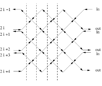
The transfer matrix of the CC model consists of local $2\times 2$ matrices of the form

$$\left(\begin{array}[]{c}w_{1R}\\ w_{2R}\end{array}\right)=\left(\begin{array}[]{cc}1/t&r/t\\ r/t&1/t\\ \end{array}\right)\left(\begin{array}[]{cc}e^{i\alpha_{1}}&0\\ 0&e^{i\alpha_{2}}\\ \end{array}\right)\left(\begin{array}[]{c}w_{1L}\\ w_{2L}\end{array}\right)\ ,$$ (9)

where $t=1/\sqrt{1+e^{2x}}$ is the tunneling amplitude of electronic states and $r=\sqrt{1-t^{2}}$ is the rotation at each node of the regular lattice shown in Fig. 1. The model parameter $x$ corresponds to the Fermi energy while phases $\alpha_{i}$ ($i=1,2$) are random variables from $0$ to $2\pi$, arising from the randomness of the potential landscape. $N$ of such local transfer matrices correspond to a vertical strip in Fig. 1 that forms $2N\times 2N$ transfer matrices $W_{1}U_{1}$ and $W_{2}U_{2}$ for neighboring columns. The parameterization of transfer matrices $W_{1}$ and $W_{2}$ in neighboring columns is such that it is invariant under the rotation by $\pi/2$, the symmetry which is obvious from Fig. 1. We therefore have two parameters $x$ and $x^{\prime}$ corresponding to neighboring columns related as follows

$$t=r^{\prime}=\frac{1}{\sqrt{1+e^{2x}}},\;\;r=t^{\prime}=\frac{1}{\sqrt{1+e^{2x^{\prime}}}}\ .$$ (10)

Figure 1: Schematic view of the CC model network structure.

The transition point $x_{c}$ is equal to $0$. As the result, matrix elements of $W_{1}$ and $W_{2}$ are defined as follows:

$$\left[W_{1}\right]_{2n+1\,2n+1}=\left[W_{1}\right]_{2n\,2n} =1/t\ ,$$

$$\left[W_{1}\right]_{2n+1\,2n}=\left[W_{1}\right]_{2n\,2n+1} =r/t\ ,$$

$$\left[W_{2}\right]_{2n-1\,2n-1}=\left[W_{2}\right]_{2n\,2n} =1/t^{\prime}\ ,$$

$$\left[W_{2}\right]_{2n-1\,2n}=\left[W_{2}\right]_{2n\,2n-1} =r^{\prime}/t^{\prime}\ ,$$

$$\left[W_{2}\right]_{1\,N}=\left[W_{2}\right]_{N\,1} =r^{\prime}/t^{\prime}\ ,$$

where $n=1\dots N$ and periodic boundary conditions are imposed on $W_{2}$. Matrices $U$ have a simple diagonal form $\left[U_{1,2}\right]_{nm}=\exp{(i\alpha_{n})}\,\delta_{nm}$. The final transfer matrix $T$ can then be represented as a product $\prod_{j=1}^{L}W_{1}U_{1j}W_{2}U_{2j}$.

The largest matrix element of the transfer matrix $T$ is of the order of $\eta\sim(1+e^{2x})^{L}$, growing exponentially with the system length $L$. Because we are looking for eigenvalues of $S=TT^{\dagger}$ which are closest to unity, we need to compute $S$ with the precision of about $2\log_{10}\eta$, otherwise numbers of the order of unity are unreliable due to round-off errors. We used arbitrary precision calculations with adaptive precison increasing it gradually for each matrix product. We calculated the transfer matrix $T$ of the system of length $L$ on a grid $\{N,x\}$ using a graph-like algorithm. Instead of computing product of local transfer matrices sequentially, we calculate it on a full $k$-way tree with adaptive precision. At each node we estimated the required precision and set the involved matrices to it before multiplying them. In all calculation we used $k=7$, which allowed us to perform the vast majority of the matrix multiplications (at the leaf node level) with the machine precision. When the matrix $S=TT^{\dagger}$ was computed we used the shift-and-invert Lanczos algorithm to calculate a set of selected eigenvalues of $S$ which are closest to unity. Typically, we calculated six eigenvalues with the accuracy of $10^{-5}$, checking that these eigenvalues appeared in pairs and satisfied $\log{\lambda_{2i}}=-\log{\lambda_{2i+1}}$ (where $i=0,1,2$ and $\lambda_{1}$ is the eigenvalue closest to unity from above, i. e. $\lambda_{1}>1$). We then calculated Lyapunov exponents $-(1/2N)\log[\lambda_{i}(N,x)]$. Hereafter, we only focus on the smallest Lyapunov exponent $\gamma_{N}(x)$.

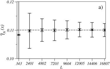
The tree-like algorithm provides access to partial transfer matrices and allows us to calculate Lyapunov exponents at different node levels, not only at the root node. The latter offers the possibility to collect and study the statistics of Lyapunov exponents. We analyzed distributions of $\gamma_{N}(x)$ for different system lengths $L$. Figure 2(a) displays the mean value $\bar{\gamma}_{N}(x)$ of the distribution and its estimated standard errors calculated for $N=60$, $x=0.404$, and $L=343,2401,\ldots,16807$. Larger error bars show the standard deviation $\sigma_{N}(x)$ of the distribution at each node (i.e., at each $L$). Smaller error bars represent the standard error of the mean value itself, estimated as

$$\bar{\sigma}_{N}(x)=\sigma_{N}(x)/\sqrt{L_{r}}\ ,$$ (11)

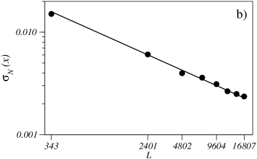
where $L_{r}$ is the size of the Lyapunov exponent ensemble at each node. Figure 2(b) demonstrates that the standard deviation $\sigma_{N}(x)$ varies as $1/\sqrt{L}$ with the system length, confirming the applicability of the central limit theorem and, hence, the definition (11).

Figure 2 shows that values of the disorder-averaged mean Lyapunov exponent for $N\geq 2401$ are the same within their error bars. We calculated these quantities for different sets of $N$ and $x$, as well as for longer chains, and found the same result. Therefore, rather than calculating the exponent for a very long chain, we can calculate the mean Lyapunov exponent for a large number $L_{r}$ of relatively short chains, which is more efficient. Varying $L_{r}$ we can achieve any given target accuracy; in our calculation we used $L=4802$ with the typical ensemble size of $N_{r}\approx 2000$.

Figure 2: a) Mean values of the $\gamma_{N}(x)$-distribution and estimated error bars calculated for $N=60$, $x=0.404$ at different node levels ($L=343,2401,\ldots,16807$). The horizontal dashed line is a guide for the eye, showing the mean value for $L=16807$. Larger error bars show the standard deviation of the distributions $\sigma_{N}(x)$, while smaller error bars are equal to $\bar{\sigma}_{N}(x)$ and estimate the error of the mean value. b) Full circles show the standard deviation $\sigma_{N}(x)$ as a function of the system length $L$ and the solid line is the best $1/\sqrt{L}$ fit to the data.

Having calculated disorder-averaged Lyapunov exponents, we use the standard FSS analysis of the data, formulated in Ref. Kramer, and extended in the Refs. Ohtsuki, ; Roemer, ; Eilmes, , in order to obtain the localization length index $\nu$. The Lyapunov exponent is believed to have scaling behavior (see for example Refs. Ohtsuki, and SO, and references therein), and finite size effects can be accounted for by the following formula for the scaling function $\Gamma(N,x)$ which approximates $N\bar{\gamma}_{N}(x)$ in the vicinity of the critical point

$$\Gamma(N,x)=F_{0}(N^{1/\nu}u_{0})+F_{1}(N^{1/\nu}u_{0})N^{y}\,u_{1}$$ (12)

where $F_{0}(\cdot)$, $F_{1}(\cdot)$, $u_{0}(\cdot)$ and $u_{1}(\cdot)$ are universal, independent of $L$ functions. The first function $F_{0}(\cdot)$ is the contribution of the main operator in the corresponding conformal field theory, which defines the correlation length. The second function $F_{1}(\cdot)$ results from the operator with the anomalous dimension which is close to that of the main one. We used the following formula to fit to the dataEilmes ; SO :

$$\Gamma(N,x)=\sum_{n=0}^{3}a_{0\,2n}\left[u_{0}(x)\,N^{1/\nu}\right]^{2n}+a_{10}\,u_{1}(x)\,N^{y}$$ (13)

where $u_{0}(x)=x+b_{3}x^{3}$ and $u_{1}(x)=1+c_{2}x^{2}$, so the series for $F_{0}$, $F_{1}$, $u_{0}$, and $u_{1}$ were truncated at orders 6, 0, 3 and 2, respectively. Further increase of these orders turned up to be impractical as it deteriorated the result.

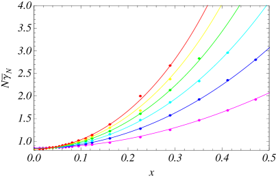
Because all mean Lyapunov exponents have different error bars we used a weighted fit with $[N\bar{\sigma}_{L}(x)]^{-2}$ as weights. We also put the following constraints on the parameters: $0.5<a_{00}<1$, $|a_{0\,2n}|,|a_{10}|,|b_{3}|,|c_{2}|\leq 2$, $2.1\leq\nu\leq 2.7$ and $-0.5\geq y\geq 0$. We checked that the result is not affected by the constraints while they stabilize the procedure and improve the convergence of the nonlinear fit. All fits which converged to a constraint boundary were discarded. Global optimization methods such as the simulated annealing were used to find the best fit. The result of such a fit is presented in Fig. 3. All curves intersect at $x\approx 0.025$; note that the ordering of the curves at $x=0$ suggests an additional constraint, namely $a_{10}>0$.

In order to estimate error bars of the parameters we used the standard resampling technique.NR Up to $1000$ generated synthetic data sets of mean Lyapunov exponents were drawn from the corresponding normal distributions centered at $\bar{\gamma}_{N}(x)$ and having the standard deviation $\bar{\sigma}_{N}(x)$. Fitting to these data we obtained distributions of the parameters and calculated their mean values and standard errors. The following parameter values were found: for the case $c_{1}\neq 0$ we obtained $\nu=2.519\pm 0.023$, $y=-0.32$ and the typical goodness of fit parameter was $\chi^{2}=864.5$ for $107$ points. For $c_{1}=0$, $\nu=2.517\pm 0.018$, $y\approx-0.24$ and $\chi^{2}=848.2$. We note that the parameter $y$ is always small, which suggests that finite size effects are very pronounced in the CC model.

The curves for Lyapunov exponents for different sizes $N$ are intersecting in a region close to $x=0$. The crossing point of a pair of such curves corresponding to consecutive values of $N$ shifts towards the origin on increasing $N$. The latter is the consequence of the condition $a_{10}>0$, which increases the role of the next to the leading operator in the problem for small $N$. This fact stresses the importance of the second operator together with the main one in the analysis of possible candidate conformal field theories which describe plateau-plateau transitions in the quantum Hall effect.

Figure 3: Simpulated data and the fit of Eq. 13 to them ($c_{1}=0$). From bottom to top (for $x>0.2$): $N=10,20,\dots,60$.

The obtained value of the critical index $\nu=2.517\pm 0.018$ disagrees with early results,BH ; Raikh ; RC which could be attributed to the quality of the data, system sizes reached, and finite size effects. Those effects prooved to be extremely important for accurate calculation of the critical exponent even in the standard Anderson model,Ohtsuki in which case the irrelevant exponent $y\sim-3$ is much larger than in the CC model (finite size effects are therefore less pronounced). On the other hand, our critical exponent is smaller than the one calculated by Slevin and Ohtsuki,SO who obtained $\nu=2.593\pm 0.006$. However, both high precision numerical results are considerably above the experimental value of $\nu=2.38\pm 0.06$ measured recently in GaAs-AlGaAs heterostructures. Li1 ; Li2 The latter fact emphasizes the necessity to investigate the validity of the CC model further.

In summary, the obtained critical exponent $\nu>2.5$ suggests that the rational value $7/3$ which is in agreement with some early calculations, could be questioned. Our technique is based on the calculation of the product of transfer matrices preserving the required precision during iterations and collecting large statistics to achieve a given target precision. Finite-size effects turn out to be very pronounced within the framework of the CC model and should be taken into account properly in order to obtain reliable results. In particular, the calculated value of the critical exponent suggests that some WZWN-type models based on the conformal field theory should be reconsidered, which demands new developments and approaches in the formulation of the continuum limit of the CC model as well as further studies and more accurate calculations of Lyapunov indices.

AS acknowledges discussions with I. Gruzberg, V. Kagalovsky and thanks for hospitality the Universidad Complutense de Madrid where the major part of the work has been done. AVM and FD-A thank K. Slevin for fruitful discussions. Part of the calculations were performed at the Aula Sun Cluster and the Clúster de Cálculo de Alta Capacidad para Técnicas Físicas, funded by the UCM and the UE under FEDER programme. Work in Madrid was supported by EC (project MOSAICO) and BSCH-UCM (project PR34/07-15916).

References

- (1) H. Levine, S. B. Libby, A. M. M. Pruisken, Phys. Rev. Lett. 51, 1915 (1983); Nucl. Phys. B 240, 30 (1984); ibid. 240, 49 (1984); ibid. 240, 71 (1984).
- (2) J. Chalker and P. Coddington, J. Phys. C 21 2665 (1988).
- (3) B. Huckenstein, Rev. Mod. Phys. 67 357 (1995).
- (4) H. P. Wei, L. W. Engel, and D. C. Tsui, Phys. Rev. B 50, 14609 (1994).
- (5) D.-H. Lee, Z. Wang, and S. Kivelson, Phys. Rev. Lett. 70, 4130 (1993).
- (6) D.-H. Lee, Phys. Rev. B 50, 10788 (1994).
- (7) D.-H. Lee and Z. Wang, Phil. Mag. Lett. 73, 145 (1996).
- (8) S. Cho and M. P. A. Fisher, Phys. Rev. B 55, 1025 (1997).
- (9) M. R. Zirnbauer, J. Math. Phys. 38 2007 (1997).
- (10) A. Sedrakyan, Phys. Rev. B68, 235329 (2003).
- (11) M. J. Bhaseen I. I. Kogan, O. A. Soloviev, N. Taniguchi, and A.M. Tsvelik, Nucl. Phys. B580, 688 (2000); A. M. Tsvelik, Phys. Rev. B 75, 184201 (2007).
- (12) A. LeClair, Phys. Rev. B 64, 045329 (2001).
- (13) H. Obuse, A. R. Subramaniam, A. Furusaki, I. A. Gruzberg, and A. W. W. Ludwig, Phys. Rev. Lett. 101, 116802 (2008).
- (14) F. Evers, A. Mildenberger, and A. D. Mirlin, Phys. Rev. Lett. 101, 116803 (2008).
- (15) V. N. Tutubalin, Theor. Proba. Appl. 10, 21 (1965).
- (16) A. MacKinnon and B. Kramer, Phys. Rev. Lett. 47, 1546 (1981).
- (17) K. Slevin, T. Ohtsuki, Phys. Rev. Lett. 78 4083, (1997); Phys. Rev. Lett. 82, 382 (1999).
- (18) F. Mildea , R.A. Römer, M. Schreiber, and V. Uski, Eur. Phys. J. B 15, 685690 (2000).
- (19) A. Eilmes, M. A. Fisher, and R. Römer, Phys. Rev. B 77, 245117 (2008)
- (20) K. Slevin and T. Ohtsuki, Phys. Rev. B 80, 041304(R) (2009).
- (21) W. Press, B. Flannery, and S. Teukolsky, Numerical Recipes in Fortran (Cambridge University Press, Cambridge, 1992), Chap. 15.
- (22) A. G. Galstyan and M. E. Raikh, Phys. Rev. B 56, 1422 (1997).
- (23) P. Cain, R. Römer, and M. E. Raikh, Phys. Rev. B. 67, 075307 (2003).
- (24) W. Li, G. A. Csathy, D. C. Tsui, L. N. Pfeiffer, and K. W. West, Phys. Rev. Lett. 94, 206807 (2005).
- (25) W. Li, C. L. Vicente, J. S. Xia, W. Pan, D. C. Tsui, L. N. Pfeiffer, and K. W. West, Phys. Rev. Lett. 102, 216801 (2009).