Temperature dependence of uniform static magnetic susceptibility in a two-dimensional quantum Heisenberg antiferromagnetic model

Abstract

A perturbation spin-wave theory for the quantum Heisenberg antiferromagnets on a square lattice is proposed to calculate the uniform static magnetic susceptibility at finite temperatures, where a divergence in the previous theories due to an artificial phase transition has been removed. To the zeroth order, the main features of the uniform static susceptibility are produced: a linear temperature dependence at low temperatures and a smooth crossover in the intermediate range and the Curie law at high temperatures. When the leading corrections from the spin-wave interactions are included, the resulting spin susceptibility in the full temperature range is in agreement with the numerical quantum Monte Carlo simulations and high-temperature series expansions.

I Introduction

The quantum Heisenberg antiferromagnet (QHAFM) is a prototype model to describe the magnetic properties in the parent compounds of high temperature superconducting cuprates.Manousakis (1991) Non-linear sigma model is shown that its ground state has long-range order and its low energy excitations are in a renormalized classical state.Chakravarty et al. (1988, 1989); Chubukov et al. (1994) These results are confirmed by the quantum Monte Carlo methodsMakivić and Ding (1991); Makivić and Jarrell (1992) and are consistent with experimental data.Chakravarty et al. (1988) Moreover, the Schwinger boson mean field theoryAuerbach and Arovas (1988); Arovas and Auerbach (1988) and the variational spin-wave theoryTakahashi (1989) have also been developed for the two-dimensional QHAFM, leading to similar conclusions. Previous theoretical studies have concentrated in the low temperature region. However, the low-energy interesting physics of the two-dimensional QHAFM can persist up to the temperature region $T\simeq J$. Moreover, the anomalous normal state in the charged doped QHAFM in the cupratesTimusk and Statt (1999) relies on a theory for the magnetic fluctuations in the intermediate temperature range. Therefore, a theory is needed to be well defined in the full temperature range.

Although the Schwinger boson mean field theoryAuerbach and Arovas (1988); Arovas and Auerbach (1988) and Takahashi’s variational spin-wave theoryTakahashi (1989) for a QHAFM in square lattices can be extended to the finite temperature range, the mean field ansatz results in a finite temperature phase transition at $T_{c}=0.91J$, which explicitly violates the Mermin-Wagner theoremMermin and Wagner (1966). To overcome this artificial mean filed divergence of the magnetic susceptibility, we will propose a perturbation spin-wave theory.

In the Takahashi’s variational spin-wave theory, the Dyson-Maleev spin-boson representation is used for the QHAFM on a square lattice with a Néel ordered ground state:

$$S_{i}^{-}=a_{i}^{{\dagger}},S_{i}^{+}=(2S-a_{i}^{{\dagger}}a_{i})a_{i},S_{i}^{z}=S-a_{i}^{{\dagger}}a_{i},$$ (1)

for the spins in the spin-up sublattice, and

$$S_{j}^{-}=b_{j},S_{j}^{+}=b_{j}^{{\dagger}}(2S-b_{j}^{{\dagger}}b_{j}),S_{j}^{z}=-S+b_{j}^{{\dagger}}b_{j},$$ (2)

for the spin-down sublattice. The Dyson-Maleev or the Holstein-Primakoff spin-wave theory works well for the ground state. The corresponding results, such as the spin-wave velocity, the spin stiffness constant, the sublattice magnetization, and the perpendicular susceptibility,Igarashi (1992); Canali et al. (1992); Weihong and Hamer (1993) agree well to the quantum Monte Carlo simulations.Sandvik (1997)

To develop a finite temperature spin-wave theory, Takahashi introduced a constraint for the vanishing local magnetization, i.e.,

$$\langle S_{l}^{z}\rangle=0$$ (3)

at the $l$’th lattice site, which automatically fulfills the Mermin-Wagner theorem. Takahashi also introduced a mean field order parameter $\langle a_{i}b_{j}\rangle=\langle a_{i}^{{\dagger}}b_{j}^{{\dagger}}\rangle$ to account for the spin-wave interaction in mean field level. This mean field ansatz can describe reliably the low temperature physics, but fails at high temperatures, where it produces an artificial phase transition.

In this paper, we present a perturbation spin-wave theory with the constraint Eq. (3). The spin-wave interactions are considered within a many-body perturbation method. The mean field divergence in the previous variational spin-wave theory is removed. To verify our perturbation spin-wave theory, we calculate the uniform static susceptibility. Its temperature dependence in the zeroth order can catch most features given by the quantum Monte Carlo simulations and high temperature series expansion. It shows a linear temperature dependence at low temperatures, a smooth crossover in the intermediate range and the Curie law at high temperatures. By including the first order corrections from the spin wave interactions, our perturbation spin-wave theory agrees quantitatively well with the numerical simulations.

This paper is organized as follows. In Sec. II, we present the linearized spin wave results up to the zeroth order. In Sec. III, a perturbation theory with the first order corrections from the spin-wave interactions are developed. We also give the comparison of the static magnetic susceptibility with the results of quantum Monte Carlo simulations and high-temperature series expansions. In Sec. IV, we give the discussion and summary.

II Linearized spin-wave theory

In this paper we mainly discuss a QHAFM on a quare lattice with Hamiltonian defined by

$$H=J\sum_{\langle ij\rangle}\mathbf{S}_{i}\cdot\mathbf{S}_{j},$$ (4)

where $J>0$ and $\langle ij\rangle$ denotes nearest-neighbor sites. Since the ground state of this QHAFM Hamiltonian is an Néel ordered state, we separate the square lattice with $2N$ sites into sublattice $A$ for the up spins and sublattice $B$ for the down spins.

The Dyson-Maleev spin representation given by Eq.(1) and (2) are defined upon the Néel ordered state. In terms of boson operators, the model can be divided into

$$H=H_{l}+H_{I},$$ (5)

where $H_{l}$ contains the classical energy and the quadratic terms,

$$H_{l} = 2JS\sum_{\langle ij\rangle}\left(a_{i}^{{\dagger}}a_{i}+b_{j}^{{\dagger}}b_{j}+a_{i}b_{j}+a_{i}^{{\dagger}}b_{j}^{{\dagger}}\right)$$ (6)

$$-NJzS^{2},$$

and $H_{I}$ contains the quartic terms, describing the spin-wave interactions,

$$H_{I}=-J\sum_{\langle ij\rangle}a_{i}^{{\dagger}}\left(a_{i}+b_{j}^{{\dagger}}\right)^{2}b_{j}.$$ (7)

In this section, we neglect the spin-wave interactions and focus on the Hamiltonian $H_{l}$. We refer this approximate to a linearized spin-wave theory (LSW). The spin-wave interaction in the Hamiltonian $H_{I}$ will be studied in Sec. III.

The constraint Eq. (3), from the Dyson-Maleev representation, can be described by introducing a Lagrangian Hamiltonian asTakahashi (1989)

$$H_{\lambda}=-\sum_{i\in A}u_{i}(S-a_{i}^{{\dagger}}a_{i})-\sum_{j\in B}u_{j}(S-b_{j}^{{\dagger}}b_{j}),$$ (8)

where the Lagrangian multipliers $\mu_{i}$ and $\mu_{j}$ are assumed to be site independent, i.e. $\mu_{i}=\mu_{j}=\mu$. Physically the Lagrangian multiplier $\mu$ plays a role of an effective chemical potential for the spin waves and leads to a finite gap, thus an effective mass, for these bosonic excitations at finite temperatures. For convenience in our following discussion, we define $\mu\equiv JzS(\lambda-1)$ with the coordinate number $z=4$.

By using the Fourier transformations and performing the Bogoliubov transformations, the Hamiltonian $H_{0}=H_{l}+H_{\lambda}$ can be expressed as

$$H_{0} = \sum_{\mathbf{k}}\varepsilon_{\mathbf{k}}\left(\alpha_{\mathbf{k}}^{{\dagger}}\alpha_{\mathbf{k}}+\beta_{\mathbf{k}}^{{\dagger}}\beta_{\mathbf{k}}\right)+\sum_{\mathbf{k}}\varepsilon_{\mathbf{k}}$$ (9)

$$-NJz\lambda S(1+2S)+NJzS^{2},$$

where $\varepsilon_{\mathbf{k}}=JzS\sqrt{\lambda^{2}-\gamma_{\mathbf{k}}^{2}}$ and $\gamma_{\mathbf{k}}=\cos\frac{1}{2}k_{x}\cos\frac{1}{2}k_{y}$. Here $\left(\alpha_{\mathbf{k}}^{{\dagger}},\alpha_{\mathbf{k}}\right)$ and $\left(\beta_{\mathbf{k}}^{{\dagger}},\beta_{\mathbf{k}}\right)$ are operators describing two branches of Bogoliubov excitations. The free energy per site is given by

$$f = \frac{T}{N}\sum_{\mathbf{k}}\ln\left(2\sinh\left(\frac{\varepsilon_{\mathbf{k}}}{2T}\right)\right)-\frac{Jz}{2}\lambda S(1+2S)$$ (10)

$$+\frac{JzS^{2}}{2},$$

Minimizing the free energy with respect to $\lambda$ leads to a self-consistent equation

$$S+\frac{1}{2}=\frac{1}{2N}\sum_{\mathbf{k}}\frac{\lambda}{\sqrt{\lambda^{2}-\gamma_{\mathbf{k}}^{2}}}\coth\left(\frac{\varepsilon_{\mathbf{k}}}{2T}\right),$$ (11)

as a consequence of the constraint Eq. (3).

The uniform static susceptibility per site can be calculated from the static spin-spin correlation function,

$$\chi(T)=\frac{1}{6NT}\sum_{lr}\langle\mathbf{S}_{l}\cdot\mathbf{S}_{l+r}\rangle_{l}.$$ (12)

Here the thermal average is defined in the zeroth order linearized spin-wave approximation as $\langle\hat{O}\rangle_{l}\equiv\frac{Tr\left(e^{-H_{0}/T}\hat{O}\right)}{Tr\left(e^{-H_{0}/T}\right)}$. It can be easily shown that the transverse spin-spin correlation function $\chi_{\perp}=\frac{1}{12NT}\sum_{lr}\langle S_{l}^{+}S_{l+r}^{-}+S_{l}^{-}S_{l+r}^{+}\rangle=0$. Therefore, only the longitudinal spin-spin correlation function $\chi_{z}=\frac{1}{6NT}\sum_{lr}\langle S_{l}^{z}S_{l+r}^{z}\rangle$ has a finite value. The vanishing transverse spin-spin correlation function can also be shown in the Takahashi’s variational spin-wave theory.Takahashi (1989) Physically it stems from the local constraint given in Eq. (3).

The longitudinal spin-spin correlation function can be calculated by introducing a weak external magnetic field $B\mathbf{e}_{z}$ along $z$-axis which introduces an additional term $H_{B}=-B\left(\sum_{i\in A}S_{i}^{z}+\sum_{j\in B}S_{j}^{z}\right)$ to the model Hamiltonian. The longitudinal static susceptibility thus reads $\chi_{z}=-\frac{\partial^{2}f(B)}{\partial B^{2}}$, where the free energy $f(B)$ includes the contribution from the external field $H_{B}$. Then the uniform static susceptibility within the linearized spin-wave theory has the form:

$$\chi_{l}(T)=\frac{1}{12NT}\sum_{\mathbf{k}}\sinh^{-2}\left(\frac{\varepsilon_{\mathbf{k}}}{2T}\right).$$ (13)

A similar expression has also been obtained by Takahashi in his variational spin-wave theory.Takahashi (1989)

II.0.1 Antiferromagnetic ordered state at zero temperature

The ground state of the QHAFM on a square lattice has a long-range orderTakahashi (1989); Hirsch and Tang (1989) due to the presence of Bose-Einstein condensation (BEC) at the momentum $\mathbf{k}=(0,0)$. Since $\lambda=1+O\left(N^{-1}\right)$ at zero temperature, the spin-wave spectrum is given by

$$\varepsilon_{\mathbf{k}}=JzS\sqrt{1-\gamma_{\mathbf{k}}^{2}}.$$ (14)

Comparing to the Takahashi’s spin wave spectrumTakahashi (1989) $\varepsilon_{MT,\mathbf{k}}=Jzm_{1}\sqrt{1-\gamma_{\mathbf{k}}^{2}}$ with $m_{1}=S+0.078974$, we find that it can be obtained by rescaling our spin-wave result as

$$\varepsilon_{MT,\mathbf{k}}=a\varepsilon_{\mathbf{k}},a=\frac{m_{1}}{S}.$$ (15)

The additional factor $a$ is the main difference at low temperatures between our linearized spin-wave theory and Takahashi’s variational theory .

The spin-spin correlation function in the long distant limit can be derived as

$$\langle\mathbf{S}_{l}\cdot\mathbf{S}_{l+\mathbf{r}}\rangle=c(\mathbf{r})\left(m_{0}+\frac{1}{2\pi r}\right)^{2},$$ (16)

where $c(\mathbf{r})=1$ if $l,l+\mathbf{r}$ are in the same sublattice, and $-1$ if $l,l+\mathbf{r}$ belong to different sublattices. $m_{0}=S-0.19660$ is the magnetization at zero temperature, which is the same as that in the Schwinger boson mean field theoryHirsch and Tang (1989). Both the spin-spin correlation function and the local spontaneous magnetization $m_{0}$ in our linearized spin-wave theory agree with those of the variational spin-wave theory.Takahashi (1989) These results imply that, to the order of $O(S^{-1})$, the spin-wave interactions have no contributions to the spontaneous magnetization and static spin-spin correlation at $T=0$K, consistent to the previous results.Castilla and Chakravarty (1991); Igarashi (1992); Weihong and Hamer (1993)

II.0.2 Paramagnetic state at finite temperatures

Figure 1: The Lagrangian multiplier $\lambda(T)$ in the linearized spin-wave theory for the QHAFM on a square lattice with different spin magnitude $S=1/2,1$ and $3/2$.

Figure 2: The uniform static magnetic susceptibility $\chi_{l}(T)$ for $S=1/2,1$ and $3/2$ in our linearized spin wave theory of the QHAFM on a square lattice.

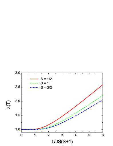
At finite temperatures, according to the Mermin-Wagner theorem, the long-range order is destroyed in the QHAFM model by quantum fluctuations.Mermin and Wagner (1966) Fig. 1 shows the temperature dependence of the Lagrangian multiplier $\lambda(T)$ with different quantum spins $S=1/2,1,3/2$. At low temperatures $T\ll JzS$, we follow the Takahashi’s method and show analytically that $\lambda$ approaches exponentially to its BEC value $1$ as

$$\lambda=1+\frac{1}{2}\left(\frac{T}{JzS}\right)^{2}\exp\left(-\frac{\pi JzSm_{0}}{T}\right).$$ (17)

The uniform static spin susceptibility in this low temperature region can also be derived analytically, leading to a linear-temperature dependence,

$$\chi_{l}(T)=\frac{m_{0}}{3JzS}+\frac{2T}{3\pi\left(JzS\right)^{2}}.$$ (18)

The first term gives a finite spin susceptibility at zero temperature. The linear term results from the linear density of states of the spin-wave excitations in the low energy limit. The low-energy spin-wave excitations at low temperatures have an approximate dispersion

$$\varepsilon_{\mathbf{k}}=JzS\sqrt{\Delta^{2}+\frac{1}{4}\mathbf{k}^{2}},$$ (19)

where a dimensionless bosonic gap is defined by $\Delta\equiv\sqrt{\lambda^{2}-1}$. At low temperatures, $\lambda$ decays exponentially to $1$ as Eq.(17), therefore the energy spectrum Eq.(19) is approximately as $\varepsilon_{\mathbf{k}}=\frac{JzS}{2}k$. The density of states $\rho(\omega)$ of the spin-wave excitations is $\rho(\omega)=\frac{1}{(2\pi)^{2}}\int d^{2}\mathbf{k}\delta\left(\omega-\varepsilon_{\mathbf{k}}\right)=\frac{2\omega}{\pi\left(JzS\right)^{2}}$. It is this linear density of states that leads to the linear-temperature dependence of the static magnetic susceptibility at low temperatures. Note that by scaling the linear temperature susceptibility $\chi_{l}(T)$ by the factor $a$, we can obtain the low-temperature susceptibility given by Takahashi,Takahashi (1989) $\chi_{MT}(T)=\frac{1}{a}\chi_{l}\left(\frac{T}{a}\right)$.

At low temperatures, the spin-spin correlation function follows

$$\langle\mathbf{S}_{i}\cdot\mathbf{S}_{i+\mathbf{r}}\rangle=c(\mathbf{r})\frac{4}{\pi}\left(\frac{T}{JzS}\right)^{2}\frac{\xi}{r}e^{-r/\xi},$$ (20)

where $c(\mathbf{r})$ is defined in Eq.(16) and $\xi$ is the correlation length defined by $\xi\equiv\frac{1}{4\sqrt{\lambda^{2}-1}}$. From Eq.(17), it can be easily shown that

$$\xi(T)=\frac{JzS}{4T}\exp\left(\frac{\pi JzSm_{0}}{2T}\right).$$ (21)

Takahashi’s result for the spin-spin correlation length $\xi_{MT}(T)$ can be obtained by rescaling with the factor $a$ defined in Eq.(15), $\xi_{MT}(T)=\xi\left(\frac{T}{a}\right)$. This exponential temperature dependence of the spin correlation length agrees with that obtained from one-loop renormalization group approach of the non-linear sigma model.Kopietz and Chakravarty (1989); Manousakis (1991) Compared to the experimental data and the numerical simulations, the two-loop approximation is necessary to convert the $1/T$ prefactor of the exponential into a constant.Chakravarty et al. (1988, 1989)

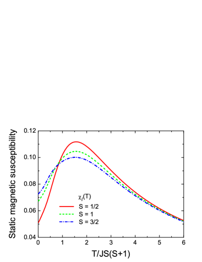
When increasing the temperature, the Lagrangian multiplier $\lambda(T)$ in Fig. 1 evolves from the low-temperature exponential behavior to the linear temperature dependence at high temperatures. At the same time, the uniform susceptibility as shown in Fig. 2 increases firstly to a broad peak at the intermediate temperature $T_{c}\propto JS(S+1)$, and then decreases at high temperatures.

At high temperatures $T\gg JzS$, the dispersion of the energy spectrum becomes relatively weak and $\lambda\gg 1$. The self-consistent equation Eq.(11) gives rise to

$$\lambda(T)=\frac{T}{JzS}\ln\left(1+\frac{1}{S}\right).$$ (22)

In the high-temperature region, the uniform static magnetic susceptibility obeys the Curie law,

$$\chi_{l}(T)=\frac{(S+1)S}{3T}.$$ (23)

Such a high-temperature Curie-law behavior in the linearized spin-wave theory is exactly the same as that in the Takahashi’s theory.Takahashi (1989) Why our linearized spin-wave theory can give rise to a Curie-law behavior, in contrast to the general spin-wave theory is a very interesting question. The basic reason is that there is an effective chemical potential introduced for our spin waves by the local constraint Eq.(3). This gives rise to a temperature dependent finite gap for the spin waves which behave as bosons with effective mass at finite temperatures.

It should be noted that in our numerical solution to the self-consistent equation Eq.(11) and in calculating the uniform magnetic susceptibility Eq.(13), there is a trick to include the contribution of the low-energy spin-wave excitations at low temperatures. Although no exact BEC occurs at finite temperatures, in the actual numerical calculation Eq.(17) shows us that the exponential decay of the bosonic gap $JzS\Delta$ at $\mathbf{k}=(0,0)$ will lead to a difficulty in numerically calculating the momentum integral from the low-energy region $\varepsilon_{\mathbf{k}}\ll T$. We call this difficulty as a BEC-like pseudo-singularity.

A trick to deal with the BEC-like pseudo-singularity is to separate the momentum space into two regions: Region (i) $\mathbf{k}\in\mathbf{k}_{BEC}+\delta_{\mathbf{k}}$ and Region (ii) is the rest part in the first Brillouin Zone. Here the momentum $\mathbf{k}\in\delta_{\mathbf{k}}$ satisfies $\left|\mathbf{k}\right|<k_{m}$. $k_{m}$ is an irrelevant parameter and we choose $k_{m}=0.01$ in our calculations. The momentum integral in Region (i) can be firstly calculated with an approximate spin-wave energy dispersion Eq.(19).

Figure 3: Comparison of the uniform static magnetic susceptibility with the $S=1/2$ linearized spin-wave theory (LSW) and the Takahashi’s variational theoryTakahashi (1989) for the QHAFM on a square lattice.

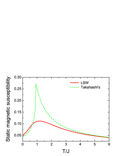
For comparison, the uniform static magnetic susceptibility from our linearized spin-wave theory and the Takahashi’s variational results are shown in Fig. 3. The sharp peak value at $T_{c}=0.91J$ in the Takahashi’s theory comes from an artificial phase transition due to vanishing of the mean-field ansatz. At low temperatures, the static magnetic susceptibility from our linearized spin-wave theory is slightly larger than the Takahashi’s result. At high temperatures, the Curie law occurs exactly in both theories. Clearly, the artificial phase transition has been removed in the linearized spin-wave theory.

One special feature in the uniform magnetic susceptibility shown in Fig. 2 is a kink structure around the temperature $T\approx 0.5JS$, where the slop of the susceptibility changes from a smaller value into a larger one. This special feature is also observed in the quantum Monte Carlo data. Kim and Troyer (1998) It was argued to originate from a crossover from a renormalized classical regime into a quantum critical regime. However, the Monte Carlo simulation shows that a similar abrupt change also appears in a classical Heisenberg model.Kim and Troyer (1998) Therefore, whether there is a crossover is still controversial. However, this kink structure implies obviously different scenarios occurring in these two temperature regions.

III First order corrections from the spin-wave interactions

In this section, we will go beyond the linearized approximation by including the first order corrections from the spin-wave interactions of the QHAFM model. The method is based on the many-body perturbation theory.

III.1 Formulation for first order corrections

After the Fourier and Bogoliubov transformations, the total Hamiltonian $H=H_{l}+H_{\lambda}+H_{I}$ can be approximated byOguchi (1960)

$$\mathcal{H} = \mathcal{H}_{0}+\mathcal{H}_{I}+E_{c},$$

$$\mathcal{H}_{0} = \sum_{\mathbf{k}}A_{\mathbf{k}}\left(n_{\mathbf{k}}+n_{\mathbf{k}}^{\prime}\right),$$

$$\mathcal{H}_{I} = \sum_{\mathbf{k}_{1},\mathbf{k}_{2}}\left[B^{\left(1\right)}\left(n_{\mathbf{k}_{1}}n_{\mathbf{k}_{2}}+n_{\mathbf{k}_{1}}^{\prime}n_{\mathbf{k}_{2}}^{\prime}\right)+B^{\left(2\right)}n_{\mathbf{k}_{1}}n_{\mathbf{k}_{2}}^{\prime}\right],$$

$$E_{c} = \sum_{\mathbf{k}}\varepsilon_{\mathbf{k}}+NJzS\left[S-\lambda\left(1+2S\right)\right]-\frac{NJz}{4}c_{1}^{2},$$ (24)

where $n_{\mathbf{k}}\equiv\alpha_{\mathbf{k}}^{{\dagger}}\alpha_{\mathbf{k}}$, $n_{\mathbf{k}}^{\prime}\equiv\beta_{\mathbf{k}}^{{\dagger}}\beta_{\mathbf{k}}$, $c_{1}(\lambda)=1-\frac{1}{N}\sum_{\mathbf{k}}\frac{\lambda-\gamma_{\mathbf{k}}^{2}}{\zeta_{\mathbf{k}}}$, $\zeta_{\mathbf{k}}=\sqrt{\lambda^{2}-\gamma_{\mathbf{k}}^{2}}$, and $A_{\mathbf{k}}=JzS\zeta_{\mathbf{k}}\left(1+c_{1}\frac{\lambda-\gamma_{\mathbf{k}}^{2}}{2S\zeta_{\mathbf{k}}^{2}}\right)$ represents the spin-wave energy spectrum with corrections from the normal ordering of $H_{I}$. At zero temperature, $\lambda=1+O\left(N^{-1}\right)$ and the spin-wave energy dispersion is given by $A_{\mathbf{k}}=JzS\zeta_{\mathbf{k}}\left(1+\frac{c_{1}\left(1\right)}{2S}\right)$ with $c_{1}\left(1\right)=0.15794$ for $S=1/2$. The parameters $B^{\left(1\right)}$ and $B^{\left(2\right)}$ are defined by

$$B^{\left(1\right)} = -\frac{Jz}{4N}\left(\frac{\left(\lambda-\gamma_{\mathbf{k}_{1}}^{2}\right)\left(\lambda-\gamma_{\mathbf{k}_{2}}^{2}\right)}{\zeta_{\mathbf{k}_{1}}\zeta_{\mathbf{k}_{2}}}-1\right),$$

$$B^{\left(2\right)} = -\frac{Jz}{2N}\left(\frac{\left(\lambda-\gamma_{\mathbf{k}_{1}}^{2}\right)\left(\lambda-\gamma_{\mathbf{k}_{2}}^{2}\right)}{\zeta_{\mathbf{k}_{1}}\zeta_{\mathbf{k}_{2}}}+1\right).$$

In the above approximation, we have ignored the off-diagonal parts in the Fock space and picked up all the terms of the two spin-wave interactions. This is enough when we only consider the first order corrections from the spin-wave interactions for the free energy, since the linked cluster theorem tells that $f=f_{0}+\langle\mathcal{H}_{I}\rangle_{0}$, where the thermal average is defined by $\langle\hat{O}\rangle_{0}\equiv\frac{Tr\left(e^{-\mathcal{H}_{0}/T}\hat{O}\right)}{Tr\left(e^{-\mathcal{H}_{0}/T}\right)}$ and $f_{0}$ is defined for the free bosons with energy spectrum $A_{\mathbf{k}}$.

The free energy per lattice site reads

$$f=\frac{T}{N}\sum_{\mathbf{k}}\ln\left[\left(1-e^{-A_{\mathbf{k}}/T}\right)\right]-\frac{Jz}{2}c_{2}^{2}+\frac{1}{2N}E_{c},$$ (25)

where $c_{2}(\lambda)=\frac{1}{N}\sum_{\mathbf{k}}\frac{\lambda-\gamma_{\mathbf{k}}^{2}}{\zeta_{\mathbf{k}}}\tilde{n}_{\mathbf{k}}$ and $\tilde{n}_{\mathbf{k}}=\left(e^{A_{\mathbf{k}}/T}-1\right)^{-1}$. Minimizing this free energy, we can obtain the following self-consistent equation for the Lagrangian multiplier $\lambda$,

$$S+\frac{1}{2} = \frac{1}{2N}\sum_{\mathbf{k}}\coth\left(\frac{A_{\mathbf{k}}}{2T}\right)\left(\frac{\lambda}{\zeta_{\mathbf{k}}}+\frac{\tilde{c}\left(\lambda-1\right)\gamma_{\mathbf{k}}^{2}}{2S\zeta_{\mathbf{k}}^{3}}\right)$$ (26)

$$+\frac{1}{N}c_{2}\sum_{\mathbf{k}}\frac{\left(\lambda-\gamma_{\mathbf{k}}^{2}\right)}{4T\sinh^{2}\left(\frac{A_{\mathbf{k}}}{2T}\right)S\zeta_{\mathbf{k}}}\frac{\partial A_{\mathbf{k}}}{\partial\lambda},$$

where $\tilde{c}(\lambda)=c_{1}(\lambda)-2c_{2}(\lambda)$ and

$$\frac{\partial A_{\mathbf{k}}}{\partial\lambda} = JzS\left(\frac{\lambda}{\zeta_{\mathbf{k}}}+c_{1}\frac{(\lambda-1)\gamma_{\mathbf{k}}^{2}}{2S\zeta_{\mathbf{k}}^{3}}\right)$$

$$-Jz\frac{\lambda-\gamma_{\mathbf{k}}^{2}}{2N\zeta_{\mathbf{k}}}\sum_{\mathbf{k}_{2}}\frac{(\lambda-1)\gamma_{\mathbf{k}_{2}}^{2}}{\zeta_{\mathbf{k}_{2}}^{3}}.$$

It should be noted that the self-consistent equation Eq.(26) is physically equivalent to the first order perturbation expansion for the constraint Eq.(3),

$$0=S-\langle a_{i}^{{\dagger}}a_{i}\rangle_{0}+\int_{0}^{1/T}d\tau\langle T_{\tau}\mathcal{H}_{I}(\tau)a_{i}^{{\dagger}}(0)a_{i}(0)\rangle_{0}.$$ (27)

The uniform static susceptibility can also be calculated from the spin-spin correlation function given in Eq.(12). When the first order corrections from the spin-wave interactions are included, the transverse static susceptibility has a small but finite contribution,

$$\chi_{\perp}\left(T\right) = \frac{2}{T}\chi_{F}^{2}\left(T\right),$$ (28)

$$\chi_{F}\left(T\right) = S+\frac{1}{2}+\frac{c_{2}}{2S}\sum_{\mathbf{k}}\frac{\left(\lambda-1\right)\gamma_{\mathbf{k}}^{2}}{\zeta_{\mathbf{k}_{2}}^{3}}$$

$$-\frac{1}{2N}\sum_{\mathbf{k}}\coth\left(\frac{A_{\mathbf{k}}}{2T}\right)\left(\frac{\lambda}{\zeta_{\mathbf{k}}}+\frac{c_{1}\left(\lambda-1\right)\gamma_{\mathbf{k}}^{2}}{2S\zeta_{\mathbf{k}}^{3}}\right).$$

In the derivation for $\chi_{\perp}$, we have used the perturbation constraint equation Eq.(27) and ignored the higher order terms of the spin-wave interactions.

The longitudinal static susceptibility can also be calculated from the free energy by introducing a weak external field Hamiltonian $H_{B}$, yielding

$$\chi_{z}\left(T\right)=\frac{1}{4NT}\sum_{\mathbf{k}}\sinh^{-2}\left(\frac{A_{\mathbf{k}}}{2T}\right)+Jz\left[c_{2}c_{4}-c_{3}^{2}\right],$$ (29)

where the second term comes from the two spin-wave interaction compared to the linearized spin-wave expression Eq.(13), and

$$c_{3}\left(\lambda\right) = \frac{1}{N}\sum_{\mathbf{k}}\frac{-\left(\lambda-\gamma_{\mathbf{k}}^{2}\right)}{4T\zeta_{\mathbf{k}}\sinh^{2}\left(\frac{A_{\mathbf{k}}}{2T}\right)},$$

$$c_{4}\left(\lambda\right) = \frac{1}{N}\sum_{\mathbf{k}}\frac{\left(\lambda-\gamma_{\mathbf{k}}^{2}\right)\coth\left(\frac{A_{\mathbf{k}}}{2T}\right)}{4T^{2}\zeta_{\mathbf{k}}\sinh^{2}\left(\frac{A_{\mathbf{k}}}{2T}\right)}.$$

The uniform static susceptibility is thus given by

$$\chi\left(T\right)=\frac{1}{3}\left[\chi_{\perp}\left(T\right)+\chi_{z}\left(T\right)\right].$$ (30)

III.2 Numerical results

The self-consistent equation Eq.(26) and the static magnetic susceptibility Eq.(30) have been numerically calculated. When the first order corrections of the spin-wave interactions are included, the temperature dependence of both the Lagrangian multiplier $\lambda$ and the uniform static magnetic susceptibility have similar behaviors to the linearized spin-wave theory.

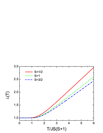
The Lagrangian multiplier $\lambda$ is shown in Fig. 4 for different spin $S=1/2,1$ and $3/2$. At low temperatures, it decays exponentially to its zero-temperature value $1$, indicating the gapless spin wave excitations. At high temperatures, $\lambda$ has a linear-temperature variation $\lambda(T)=\kappa_{0}+\kappa_{1}T$, where $\kappa_{0}$ and $\kappa_{1}$ have weak temperature dependence. For $S=1/2$, $\kappa_{0}=0.334$ and $\kappa_{1}=0.583$ in the temperature region $3J<T<10J$.

Figure 4: The Lagrangian multiplier in our perturbation spin-wave theory with the first order corrections from the spin-wave interactions.

The static magnetic susceptibility is displayed in Fig. 5. It has three main features: (i) the linear-temperature behavior at low temperatures, (ii) a broad peak at an intermediate characteristic temperature $T_{c}\propto JS(S+1)$, (iii) the Curie-Weiss law at high temperatures. For $S=1/2$, a low-temperature linear behavior can be fitted by $\chi(T)=\chi_{c}+bT$, with $\chi_{c}=0.0418$ and $b=0.0471$. Compared to the Takahashi’s theory where a similar linear behavior with $\chi_{c}=0.0437$ and $b=0.0396$,Takahashi (1989) our zero temperature susceptibility $\chi_{c}$ is slightly smaller than that of Takahashi’s. Also the slope $b$ is also slightly larger than that of the Takahashi’s.

Figure 5: The static magnetic susceptibility with different spin $S=1/2,1$ and $3/2$ in our perturbation spin-wave theory with the first order corrections from the spin-wave interactions.

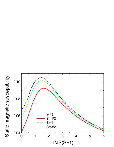
At high temperatures, the spin-wave interactions modify the exact Curie law of the static magnetic susceptibility Eq.(23) into a Curie-Weiss behavior. As shown in Fig. 6, it evolves into the behavior obtained from the numerical high-temperature series expansions. Physical origin of the high-temperature Curie-Weiss law also comes from the linear-temperature dependence of Lagrangian multiplier $\lambda$ in the energy spectrum of the spin waves.

It should be noted that the kink structure in the static magnetic susceptibility in the linearized spin-wave theory shown in Fig. 2 also occurs in the perturbation theory. This implies that the kink feature is a characteristic property in the QHAFM model.

Figure 6: Comparison of the uniform static susceptibilities from the linearized spin-wave theory (LSW) and the perturbation spin-wave theory (PSW) with first order correction for the QHAFM on a square lattice. We also show the result from the Takahashi’s modified spin-wave theory and numerical data from Quantum Monte Carlo and high-temperature series expansions (HTSE). The inset shows the comparison of PSW with HTSE in high temperature region. QMC^a comes from Ref. Kim and Troyer, 1998 and QMC^b comes from Ref. Makivić and Ding, 1991. HTSE comes from Eq.($34$) of Ref. Takahashi, 1989. For comparison, QMC^b have been multiplied by a factor $\frac{1}{3}$.

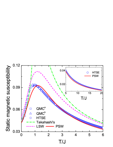
In Fig. 6, we compare the static magnetic susceptibility of our spin-wave theory to the quantum Monte Carlo dataKim and Troyer (1998); Makivić and Ding (1991) and the high-temperature series expansions. It shows that our linearized spin-wave theory can reproduce all the main features in the numerical simulations: the low temperature linear behavior, the smooth crossover in the intermediate temperature region and the Curie-Weiss law behavior at high temperature. This good agreement encourages us to study the frustrated $J_{1}-J_{2}$ model proposed to describe the magnetic fluctuation in the newly discovered iron-pnictide superconductors.Zhang et al. (2009) The first order correction from the spin-wave interactions makes the uniform static susceptibility both at low and high temperatures agrees quantitatively with the numerical quantum Monte Carlo and high temperature series expansions. This good fitting in Fig. 6 indicates that the physics of QHAFM model, at least to the static magnetic response, has been captured by our perturbation spin-wave theory in the full temperature region.

IV Discussions and Conclusions

The good agreement of our perturbation spin-wave theory with the numerical simulations shows the validity of our theory at finite temperatures. It seems surprising because the spin-wave theory developed in the pioneering papersBloch (1926); Holstein and Primakoff (1940); Anderson (1952); Kubo (1952) is generally thought to work well only at low temperatures in the ordered phase. The main difference of our finite temperature spin-wave theory is the requirement of the vanishing local magnetization. It is this local constraint that restricts the number of the spin wave excitations which thus behaves as bosons with an effective mass at finite temperatures.

The extension of the spin-wave theory to the low-dimensional spin systems have been shown to work well. In one-dimensional quantum magnets, no magnetic order can survive at zero temperature due to the strong quantum fluctuations. Although there is no long range order in the ground state, the free energy and the static magnetic susceptibility of the one-dimensional ferromagnet from a modified spin-wave theory show same behaviors to Bethe-Ansatz solutions.Takahashi (1987) The Haldane gap for the one-dimensional quantum antiferromagnet with $S=1$ from a spin-wave theory is $\Delta_{H}=0.3914J$ (Ref. Wang et al., 1994) which well agrees with the numerical density-matrix renormalization group ($0.4105J$ from Ref. White and Huse, 1993). The spin-wave theory for the one-dimensional quantum antiferromagnet with integral spin can reproduce the static magnetic susceptibility which agrees well with the quantum Monte Carlo simulations.Yamamoto and Hori (2003) These previous results, together with our study, indicate that the formulation of the spin-wave theory is a valid formalism to apply to the low-dimensional quantum magnets.

In summary, we have studied the QHAFM on a square lattice by using a perturbation spin-wave theory. The Lagrangian constraint for the absence of the local magnetization plays an important role and leads to an effective mass for the spin wave excitations at finite temperatures. In linearized spin-wave theory, the calculation of the uniform static magnetic susceptibility can reproduce almost all features obtained from the quantum Monte Carlo and the high-temperature series expansions. It has a linear-temperature dependence at low temperatures and a broad peak feature at an intermediate characteristic temperature $T_{c}\propto JS(S+1)$. At high temperatures, the uniform magnetic susceptibility follows a Curie-Weiss law. The static magnetic susceptibility from our perturbation theory with the first corrections from the spin-wave interactions agrees well with the numerical simulations.