Non-Gaussianity from Axion Monodromy Inflation

Steen Hannestad1***sth@phys.au.dk, Troels Haugbølle1,2,3haugboel@nbi.ku.dk, Philip R. Jarnhus1pjarn@phys.au.dk, and Martin S. Sloth4§§§martin.sloth@cern.ch 1 Department of Physics and Astronomy, University of Aarhus, DK-8000 Aarhus C, Denmark 2 Niels Bohr Institute, University of Copenhagen, Juliane Maries Vej 30, 2100 København Ø, Denmark 3 Niels Bohr International Academy, Blegedamsvej 17, 2100 København Ø, Denmark 4CERN, Physics Department, Theory Unit, CH-1211 Geneva 23, Switzerland
Abstract

We study the primordial non-Gaussinity predicted from simple models of inflation with a linear potential and superimposed oscillations. This generic form of the potential is predicted by the axion monodromy inflation model, that has recently been proposed as a possible realization of chaotic inflation in string theory, where the monodromy from wrapped branes extends the range of the closed string axions to beyond the Planck scale. The superimposed oscillations in the potential can lead to new signatures in the CMB spectrum and bispectrum. In particular the bispectrum will have a new distinct shape. We calculate the power spectrum and bispectrum of curvature perturbations in the model, as well as make analytic estimates in various limiting cases. From the numerical analysis we find that for a wide range of allowed parameters the model produces a feature in the bispectrum with fNL550similar-tosubscript𝑓NL550f_{\mathrm{NL}}\sim 5-50 or larger while the power spectrum is almost featureless. This model is therefore an example of a string-inspired inflationary model which is testable mainly through its non-Gaussian features. Finally we provide a simple analytic fitting formula for the bispectrum which is accurate to approximately 5 % in all cases, and easily implementable in codes designed to provide non-Gaussian templates for CMB analyses.

CERN-PH-TH/2009-253


1 Introduction

In recent years there has been an increasing interest in the primordial non-Gaussianity predicted from inflation. Single field slow-roll inflation generally predicts non-Gaussianities to be unobservably small with present day techniques [1, 2, 3, 4]. However, in non-minimal models of inflation the non-Gaussian signatures can be observable and non-Gaussianity is therefore an interesting observational window into the complexity of inflation.

Both from an observational and theoretical point of view the effective model of inflation is still uncertain. Since we do not know the microscopic origin of the effective theory of inflation, then the simplest theory of single field slow-roll inflation seems preferred from an Occam’s razor point of view. Thus, with no prejudice about the underlying microscopic theory of inflation, we do not expect large non-Gaussianities. On the other hand, when inflation is embedded into a fundamental theory like string theory, it typically carries with it more complicated structures, and therefore from a model building point of view more complicated models of inflation can be attractive.

The simplest possible model of inflation, which is a single field model of chaotic inflation with a monomial potential, requires the field values of the inflaton to be trans-Planckian. This means that higher dimensional operators has to be prohibited by some symmetry in order not to destroy the flatness of the potential. In Natural Inflation models [5, 6] this is achieved by introducing an approximate shift symmetry, and assuming that the inflaton is the pseudo-Nambu-Goldstone boson mode (axion) of the theory. It has generally been considered non-straightforward to realize this idea in string theory, because the field values would typically be restricted to sub-Plackian values. This has led to the proposal that one could extend the field range by having many axions [7]. Recently another proposal has appeared***Alternative proposals have also been promoted in [8, 9, 10], where the field range is extended by a so called monodromy mechanism [11, 12]. While not generic in this model, the model can have interesting oscillatory features embedded on top of the linear inflaton potential, depending on the details of the compactification [13].

Oscillatory features in the inflaton potential has already been studied by Chen, Easther and Lim as a way of generating large non-Gaussianity by a kind of resonance effect [14]. The axion monodromy inflation model is a concrete model, which could lead to an observational signature of this particular type of non-Gaussinity. Since the small oscillations in the potential will be very hard to detect directly in the power spectrum, the signature in the bispectrum may provide the best way of experimentally verify such a scenario.

Non-Gaussianity typically manifests itself through a non-vanishing three-point correlation function of the curvature perturbation, and is generally quantised in terms of fNLsubscript𝑓𝑁𝐿f_{NL}, which measures the deviation in the curvature perturbation ζ𝜁\zeta from a Gaussian distributed variable ζgsubscript𝜁𝑔\zeta_{g} through [2]

ζ=ζg35fNLζg2.𝜁subscript𝜁𝑔35subscript𝑓𝑁𝐿superscriptsubscript𝜁𝑔2\zeta=\zeta_{g}-\frac{3}{5}f_{NL}\zeta_{g}^{2}~{}. (1)

At present, there are only good observational constraints on a scale independent fNLsubscript𝑓𝑁𝐿f_{NL} (fNLlocalsuperscriptsubscript𝑓𝑁𝐿𝑙𝑜𝑐𝑎𝑙f_{NL}^{local}), which gives 10<fNLlocal<70superscriptsimilar-to10superscriptsubscript𝑓𝑁𝐿𝑙𝑜𝑐𝑎𝑙superscriptsimilar-to70-10~{}\mbox{\raisebox{-2.58334pt}{$\stackrel{{\scriptstyle<}}{{\sim}}$}}~{}f_{NL}^{local}~{}\mbox{\raisebox{-2.58334pt}{$\stackrel{{\scriptstyle<}}{{\sim}}$}}~{}70 at 95% C.L. [15, 16, 17, 18, 19] (note the preference for fNLlocal>0superscriptsubscript𝑓NLlocal0f_{\rm NL}^{\rm local}>0 which in some analyses is significant at more than 95% C.L.), but in the present model fNLsubscript𝑓𝑁𝐿f_{NL} will be scale dependent, and it is not clear how the bounds on fNLlocalsuperscriptsubscript𝑓𝑁𝐿𝑙𝑜𝑐𝑎𝑙f_{NL}^{local} translate into a bound on the fNLsubscript𝑓𝑁𝐿f_{NL} in the present model, but one presumingly loose some sensitivity by only constraining fNLlocalsuperscriptsubscript𝑓𝑁𝐿𝑙𝑜𝑐𝑎𝑙f_{NL}^{local} experimentially.

In the axion monodromy model, there are also non-trivial features in the power spectrum, and in the usual definition of fNLsubscript𝑓𝑁𝐿f_{NL} the power spectrum can therefore introduce some spurious scale dependence, which is not coming from the three-point function. Though this effect is at less than the per cent level for the specific models considered in this paper, we discuss a suitable alternative.

In order to calculate quantitatively the bispectrum in the axion monodromy inflation model, we have developed a code for computing non-Gaussianity in general models of single field inflation with a minimal kinetic term.

2 Bispectra in single field inflation

In the case of single field inflation with some generic potential, one can write the minimally coupled Einstein-Hilbert action as

S=d4xg[12R12(ϕ)2V(ϕ)].𝑆superscriptd4𝑥𝑔delimited-[]12𝑅12superscriptitalic-ϕ2𝑉italic-ϕS=\int\mathrm{d}^{4}x\sqrt{g}\left[\frac{1}{2}R-\frac{1}{2}(\partial\phi)^{2}-V(\phi)\right]~{}. (2)

At zeroth order, this leads to the ordinary background equation of motion for the scalar field

ϕ′′+2aaϕ+1a2dVdϕ=0superscriptitalic-ϕ′′2superscript𝑎𝑎superscriptitalic-ϕ1superscript𝑎2𝑑𝑉𝑑italic-ϕ0\phi^{\prime\prime}+2\frac{a^{\prime}}{a}\phi^{\prime}+\frac{1}{a^{2}}\frac{dV}{d\phi}=0 (3)

and the time evolution of the slow-roll background can typically be expanded in the small slow-roll parameters

ϵitalic-ϵ\displaystyle\epsilon H˙H2=12ϕ˙2H2absent˙𝐻superscript𝐻212superscript˙italic-ϕ2superscript𝐻2\displaystyle\equiv-\frac{\dot{H}}{H^{2}}=\frac{1}{2}\frac{\dot{\phi}^{2}}{H^{2}} (4)
η𝜂\displaystyle\eta ϵ˙ϵH=2ϕ¨Hϕ˙+2ϵabsent˙italic-ϵitalic-ϵ𝐻2¨italic-ϕ𝐻˙italic-ϕ2italic-ϵ\displaystyle\equiv\quad\!\!\frac{\dot{\epsilon}}{\epsilon H}=2\frac{\ddot{\phi}}{H\dot{\phi}}+2\epsilon (5)

where Ha˙/a𝐻˙𝑎𝑎H\equiv\dot{a}/a is the Hubble parameter.

Since we want to calculate correlation functions of fluctuations around this background, it is convenient to apply the ADM formalism [20]. Here the perturbed metric takes the form

ds2=N2dt2+hij(dxi+Nidt)(dxj+Njdt)𝑑superscript𝑠2superscript𝑁2𝑑superscript𝑡2subscript𝑖𝑗𝑑superscript𝑥𝑖superscript𝑁𝑖𝑑𝑡𝑑superscript𝑥𝑗superscript𝑁𝑗𝑑𝑡ds^{2}=-N^{2}dt^{2}+h_{ij}(dx^{i}+N^{i}dt)(dx^{j}+N^{j}dt) (6)

where the lapse and the shift N,Ni𝑁superscript𝑁𝑖N,N^{i} acts as Langrange multipliers when the perturbed metric is inserted into the action. Only ϕitalic-ϕ\phi and hijsubscript𝑖𝑗h_{ij} are dynamical variables, and in a convenient gauge that fix time and spatial reparametrizations, one can write

hij=a2(t)[e2ζδij+γij],subscript𝑖𝑗superscript𝑎2𝑡delimited-[]superscript𝑒2𝜁subscript𝛿𝑖𝑗subscript𝛾𝑖𝑗h_{ij}=a^{2}(t)\left[e^{2\zeta}\delta_{ij}+\gamma_{ij}\right]~{}, (7)

while having no fluctuations in the inflaton field. The physical degrees of freedom in this gauge are the scalar curvature perturbation ζ𝜁\zeta and the transverse and traceless tensor mode γijsubscript𝛾𝑖𝑗\gamma_{ij}. We can safely ignore tensor perturbation in this work, as any contribution from tensor perturbations to the scalar three-function only arise through loop diagrams.

Inserting the perturbed gauge fixed metric into the action, we can derive the action for the curvature perturbation iteratively to any order in perturbation theory. From the quadratic action of ζ𝜁\zeta

S=12dtd3xϕ˙2H2[a2ζ˙2a(ζ)2],𝑆12differential-d𝑡superscriptd3𝑥superscript˙italic-ϕ2superscript𝐻2delimited-[]superscript𝑎2superscript˙𝜁2𝑎superscript𝜁2S=\frac{1}{2}\int\mathrm{d}t\mathrm{d}^{3}x\frac{\dot{\phi}^{2}}{H^{2}}\left[a^{2}\dot{\zeta}^{2}-a(\partial\zeta)^{2}\right]~{}, (8)

upon quantizing the ζ𝜁\zeta field in the Bunch-Davies vacuum, one obtains the power spectrum, Pζ(k)subscript𝑃𝜁𝑘P_{\zeta}(k), of curvature perturbations

ζ𝐤1ζ𝐤2(2π)3δ3(𝐤1+𝐤2)Pζ(k),delimited-⟨⟩subscript𝜁subscript𝐤1subscript𝜁subscript𝐤2superscript2𝜋3superscript𝛿3subscript𝐤1subscript𝐤2subscript𝑃𝜁𝑘\left<\zeta_{{\bf k}_{1}}\zeta_{{\bf k}_{2}}\right>\equiv(2\pi)^{3}\delta^{3}({\bf{k}}_{1}+{\bf{k}}_{2})P_{\zeta}(k)~{}, (9)

which is related to the usual scale independent power spectrum by Pζ(k)=(2π2)/k3𝒫ζ(k)subscript𝑃𝜁𝑘2superscript𝜋2superscript𝑘3subscript𝒫𝜁𝑘P_{\zeta}(k)=(2\pi^{2})/k^{3}\mathcal{P}_{\zeta}(k).

Similarly one can define the bispectrum Bζsubscript𝐵𝜁B_{\zeta} by

ζ(𝐤1)ζ(𝐤2)ζ(𝐤3)(2π)3δ(a𝐤a)Bζ(𝐤1,𝐤2,𝐤3),delimited-⟨⟩𝜁subscript𝐤1𝜁subscript𝐤2𝜁subscript𝐤3superscript2𝜋3𝛿subscript𝑎subscript𝐤𝑎subscript𝐵𝜁subscript𝐤1subscript𝐤2subscript𝐤3\langle\zeta(\bm{\mathrm{{k}}}_{1})\zeta(\bm{\mathrm{{k}}}_{2})\zeta(\bm{\mathrm{{k}}}_{3})\rangle\equiv(2\pi)^{3}\delta(\sum_{a}\bm{\mathrm{{k}}}_{a})B_{\zeta}(\bm{\mathrm{{k}}}_{1},\bm{\mathrm{{k}}}_{2},\bm{\mathrm{{k}}}_{3})~{}, (10)

The strength of the non-Gaussian signal in the bispectrum can conveniently parameterised in terms of the scale independent non-linearity parameter fNLsubscript𝑓NLf_{\mathrm{NL}}, by defining

Bζ65fNL[Pζ(k1)Pζ(k2)+2 permutations].subscript𝐵𝜁65subscript𝑓NLdelimited-[]subscript𝑃𝜁subscript𝑘1subscript𝑃𝜁subscript𝑘22 permutationsB_{\zeta}\equiv\frac{6}{5}f_{\mathrm{NL}}[P_{\zeta}(k_{1})P_{\zeta}(k_{2})+\mbox{2 permutations}]\,. (11)

Now, in order to calculate the three-point function one calculates the action for the curvature perturbations, ζ𝜁\zeta, to third orderThe fourth order action has been calculated in [21], [3], [22]. , which, up to total derivatives, leads to the interaction Hamiltonian [2]

Hint(τ)subscript𝐻𝑖𝑛𝑡𝜏\displaystyle H_{int}(\tau) =\displaystyle= d3x[aϵ2ζζ2+aϵ2ζ(ζ)22ϵζ(ζ)(χ)\displaystyle-\int\mathrm{d}^{3}x\left[a\epsilon^{2}\zeta\zeta^{\prime 2}+a\epsilon^{2}\zeta(\partial\zeta)^{2}-2\epsilon\zeta^{\prime}(\partial\zeta)(\partial\chi)\right. (12)
+a2ϵηζ2ζ+ϵ2a(ζ)(χ)(2χ)+ϵ4a(2ζ)(χ)2],\displaystyle\left.+\frac{a}{2}\epsilon\eta^{\prime}\zeta^{2}\zeta^{\prime}+\frac{\epsilon}{2a}(\partial\zeta)(\partial\chi)(\partial^{2}\chi)+\frac{\epsilon}{4a}(\partial^{2}\zeta)(\partial\chi)^{2}\right]~{},

where 2χ=ϵζ˙superscript2𝜒italic-ϵ˙𝜁\partial^{2}\chi=\epsilon\dot{\zeta}.

One can, through this result, evaluate the three-point function of curvature perturbations after horizon exit, by means of the in-in formalism:

ζk1(τ)ζk2(τ)ζk3(τ)=iτ0τdτa[ζk1(τ)ζk2(τ)ζk3(τ),Hint(τ)],delimited-⟨⟩subscript𝜁subscript𝑘1𝜏subscript𝜁subscript𝑘2𝜏subscript𝜁subscript𝑘3𝜏𝑖superscriptsubscriptsubscript𝜏0𝜏differential-d𝜏𝑎delimited-⟨⟩subscript𝜁subscript𝑘1𝜏subscript𝜁subscript𝑘2𝜏subscript𝜁subscript𝑘3𝜏subscript𝐻𝑖𝑛𝑡superscript𝜏\left<\zeta_{k_{1}}(\tau)\zeta_{k_{2}}(\tau)\zeta_{k_{3}}(\tau)\right>=-i\int_{\tau_{0}}^{\tau}\mathrm{d}\tau a\left<[\zeta_{k_{1}}(\tau)\zeta_{k_{2}}(\tau)\zeta_{k_{3}}(\tau),H_{int}(\tau^{\prime})]\right>~{}, (13)

together with a field redefinition accounting for boundary terms that was neglected in eq. (12)

ζk1(τ)ζk2(τ)ζk3(τ)=ζ~k1(τ)ζ~k2(τ)ζ~k3(τ)+ηζ~k12(τ)ζ~k2(τ)ζ~k3(τ)+sym..delimited-⟨⟩subscript𝜁subscript𝑘1𝜏subscript𝜁subscript𝑘2𝜏subscript𝜁subscript𝑘3𝜏delimited-⟨⟩subscript~𝜁subscript𝑘1𝜏subscript~𝜁subscript𝑘2𝜏subscript~𝜁subscript𝑘3𝜏𝜂delimited-⟨⟩subscriptsuperscript~𝜁2subscript𝑘1𝜏subscript~𝜁subscript𝑘2𝜏subscript~𝜁subscript𝑘3𝜏sym.\left<\zeta_{k_{1}}(\tau)\zeta_{k_{2}}(\tau)\zeta_{k_{3}}(\tau)\right>=\left<\tilde{\zeta}_{k_{1}}(\tau)\tilde{\zeta}_{k_{2}}(\tau)\tilde{\zeta}_{k_{3}}(\tau)\right>+\eta\left<\tilde{\zeta}^{2}_{k_{1}}(\tau)\tilde{\zeta}_{k_{2}}(\tau)\tilde{\zeta}_{k_{3}}(\tau)\right>+\textrm{sym.}~{}. (14)

In a scenario where there are periodic ripples in the inflaton potential, the slow-roll parameters will generally oscillate. In such a scenario, it was demonstrated by Chen, Easther and Lim [14] that when the perturbations modes are inside the horizon and oscillate, they can interfere constructively with the oscillations in the couplings in the interaction Hamiltonian above, which are determined by the slow-roll parameters ϵitalic-ϵ\epsilon, ηsuperscript𝜂\eta^{\prime}. As a consequence there can be a resonant amplification of non-Gaussianity from the bispectrum.

3 The effective model of inflation from axion monodromy

It has been demonstrated that in the large field limit, which is valid during inflation, the axion monodromy model is described by a linear potential for the axion ϕitalic-ϕ\phi and an axion action of the form [12]

Sϕ=d4xg(12(ϕ)2μ3ϕ)+corrections.subscript𝑆italic-ϕsuperscriptd4𝑥𝑔12superscriptitalic-ϕ2superscript𝜇3italic-ϕcorrectionsS_{\phi}=\int\mathrm{d}^{4}x\sqrt{g}\left(\frac{1}{2}(\partial\phi)^{2}-\mu^{3}\phi\right)+{\rm corrections}~{}. (15)

One can show that in order to obtain 60 e-folds of inflation with the right level of curvature perturbations in the leading order linear potential, one should have

ϕitalic-ϕ\displaystyle\phi similar-to\displaystyle\sim 11Mpl11subscript𝑀pl\displaystyle 11M_{{\rm pl}} (16)
μ𝜇\displaystyle\mu similar-to\displaystyle\sim 6×10⁴Mpl6superscript104subscript𝑀pl\displaystyle 6\times 10^{-4}M_{{\rm pl}} (17)

as initial conditions. Though the brane-induced inflaton potential described above is the leading effect for breaking shift symmetries in the class of models considered here, there are other effect present as well. Among the more important is production of instantons, which, in this case, give rise to periodic corrections to the potential. One can therefore write down the effective potential containing these two contributions as [12]

Veff=μ3ϕ(1+α1cos(ϕ/f))+α2Ms4cos(ϕ/f),subscript𝑉𝑒𝑓𝑓superscript𝜇3italic-ϕ1subscript𝛼1italic-ϕ𝑓subscript𝛼2superscriptsubscript𝑀𝑠4italic-ϕ𝑓V_{eff}=\mu^{3}\phi(1+\alpha_{1}\cos(\phi/f))+\alpha_{2}M_{s}^{4}\cos(\phi/f)~{}, (18)

where Mssubscript𝑀𝑠M_{s} is the string scale and αisubscript𝛼𝑖\alpha_{i} are dimensionless parameters which are expected to be much smaller than one, αi1much-less-thansubscript𝛼𝑖1\alpha_{i}\ll 1, depending on the details of the string theory compactifications.

We will study the two cases α1α2much-less-thansubscript𝛼1subscript𝛼2\alpha_{1}\ll\alpha_{2} and α1α2much-greater-thansubscript𝛼1subscript𝛼2\alpha_{1}\gg\alpha_{2}, leading to two limiting potentials. For α1α2much-greater-thansubscript𝛼1subscript𝛼2\alpha_{1}\gg\alpha_{2}

Veff(1)=μ3ϕ(1+αcos(ϕ/f)),subscriptsuperscript𝑉1𝑒𝑓𝑓superscript𝜇3italic-ϕ1𝛼italic-ϕ𝑓V^{(1)}_{eff}=\mu^{3}\phi(1+\alpha\cos(\phi/f)), (19)

where we will assume αα1105𝛼subscript𝛼1similar-tosuperscript105\alpha\equiv\alpha_{1}\sim 10^{-5}, such that effect on the power spectrum is at the per cent level and not yet excluded by data. The other case is α1α2much-less-thansubscript𝛼1subscript𝛼2\alpha_{1}\ll\alpha_{2} where

Veff(2)=μ3ϕ+Λ4cos(ϕ/f),subscriptsuperscript𝑉2𝑒𝑓𝑓superscript𝜇3italic-ϕsuperscriptΛ4italic-ϕ𝑓V^{(2)}_{eff}=\mu^{3}\phi+\Lambda^{4}\cos(\phi/f), (20)

and where we will assume Λ4=α2Ms4superscriptΛ4subscript𝛼2superscriptsubscript𝑀𝑠4\Lambda^{4}=\alpha_{2}M_{s}^{4} is such that the effect on the power spectrum is at the per cent level.

The scalar power spectrum for the potential in the second model was computed analytically in [13]. We will return to this point later in Eq. (36).

3.1 Isosceles limit estimates of the bispectrum

As discussed in section two, one can write fNLsubscript𝑓𝑁𝐿f_{NL} as a combination of the three-point function of the Fourier transform of ζ𝜁\zeta and the power spectra of the curvature perturbations, yielding

fNL=103(k1k2k3)3𝒫(k1)𝒫(k2)k33+2perms.ζ𝒌1ζ𝒌2ζ𝒌3(2π)7δ(3)(𝒌1+𝒌2+𝒌3),f_{NL}=-\frac{10}{3}\frac{(k_{1}k_{2}k_{3})^{3}}{\mathcal{P}(k_{1})\mathcal{P}(k_{2})k_{3}^{3}+{\rm 2\,perms.}}\frac{\left<\zeta_{\bm{k}_{1}}\zeta_{\bm{k}_{2}}\zeta_{\bm{k}_{3}}\right>}{(2\pi)^{7}\delta^{(3)}\left(\bm{k}_{1}+\bm{k}_{2}+\bm{k}_{3}\right)}~{}, (21)

where kisubscript𝑘𝑖k_{i} is the magnitude of the momentum 𝒌isubscript𝒌𝑖\bm{k}_{i}. For the case of our models the fluctuations in the power spectrum is of the order one per cent. However if one should concern oneself with models with larger fluctuations in the power spectrum, one may benefit from using a similar definition, given by

f~NL=103(k1k2k3)3𝒫~2(k13+k23+k33)ζ𝒌1ζ𝒌2ζ𝒌3(2π)7δ(3)(𝒌1+𝒌2+𝒌3),subscript~𝑓𝑁𝐿103superscriptsubscript𝑘1subscript𝑘2subscript𝑘33superscript~𝒫2superscriptsubscript𝑘13superscriptsubscript𝑘23superscriptsubscript𝑘33delimited-⟨⟩subscript𝜁subscript𝒌1subscript𝜁subscript𝒌2subscript𝜁subscript𝒌3superscript2𝜋7superscript𝛿3subscript𝒌1subscript𝒌2subscript𝒌3\tilde{f}_{NL}=-\frac{10}{3}\frac{(k_{1}k_{2}k_{3})^{3}}{\tilde{\mathcal{P}}^{2}(k_{1}^{3}+k_{2}^{3}+k_{3}^{3})}\frac{\left<\zeta_{\bm{k}_{1}}\zeta_{\bm{k}_{2}}\zeta_{\bm{k}_{3}}\right>}{(2\pi)^{7}\delta^{(3)}\left(\bm{k}_{1}+\bm{k}_{2}+\bm{k}_{3}\right)}~{}, (22)

where 𝒫~~𝒫\tilde{\mathcal{P}} is approximately the amplitude of the power spectrum at the k𝑘k’s considered. It should be noted that this definition reduces to the 𝒢k1k2k3𝒢subscript𝑘1subscript𝑘2subscript𝑘3\frac{\mathcal{G}}{k_{1}k_{2}k_{3}} presented in [14] in the equilateral limit, but differs in the squeezed limit, where 𝒢k1k2k3𝒢subscript𝑘1subscript𝑘2subscript𝑘3\frac{\mathcal{G}}{k_{1}k_{2}k_{3}} grows as k1k3subscript𝑘1subscript𝑘3\frac{k_{1}}{k_{3}} for triangles of the type k1=k2k3subscript𝑘1subscript𝑘2much-greater-thansubscript𝑘3k_{1}=k_{2}\gg k_{3}.

We proceed to find an estimate for the case k1=k2k3subscript𝑘1subscript𝑘2subscript𝑘3k_{1}=k_{2}\geq k_{3}. Though such an estimate does not exist in general, we can obtain one by interpolating between the equilateral limit (k1=k2=k3subscript𝑘1subscript𝑘2subscript𝑘3k_{1}=k_{2}=k_{3}) and the squeezed limit (k1=k2k3subscript𝑘1subscript𝑘2much-greater-thansubscript𝑘3k_{1}=k_{2}\gg k_{3}).

3.1.1 Equilateral Limit

The model is essentially a linear slow-roll potential with a small oscillating perturbation. We can therefore follow the approach of Chen, Easther and Lim [14] and calculate the first order effect of the small oscillating term as a small correction. In this way one has ϵ=ϵ0+ϵoscitalic-ϵsubscriptitalic-ϵ0subscriptitalic-ϵ𝑜𝑠𝑐\epsilon=\epsilon_{0}+\epsilon_{osc}, η=η0+ηosc𝜂subscript𝜂0subscript𝜂𝑜𝑠𝑐\eta=\eta_{0}+\eta_{osc}. As the background solution (subscript 0), one can start from

3Hϕ˙+μ3=03𝐻˙italic-ϕsuperscript𝜇303H\dot{\phi}+\mu^{3}=0 (23)

to obtain

ϕ0=122/3(3μ3/2t+2ϕi3/2)2/3subscriptitalic-ϕ01superscript223superscript3superscript𝜇32𝑡2superscriptsubscriptitalic-ϕ𝑖3223\phi_{0}=\frac{1}{2^{2/3}}(-\sqrt{3}\mu^{3/2}t+2\phi_{i}^{3/2})^{2/3} (24)

and

ϵ0=12ϕ02,η0=2ϕ02.formulae-sequencesubscriptitalic-ϵ012superscriptsubscriptitalic-ϕ02subscript𝜂02superscriptsubscriptitalic-ϕ02\epsilon_{0}=\frac{1}{2\phi_{0}^{2}}~{},\qquad\eta_{0}=\frac{2}{\phi_{0}^{2}}~{}. (25)

As argued in [14] one can estimate fNLsubscript𝑓𝑁𝐿f_{NL} in the equilateral limit by

fNL(eq)fA(eq)sin(lnKϕf+phase)similar-tosuperscriptsubscript𝑓NL𝑒𝑞superscriptsubscript𝑓𝐴𝑒𝑞𝐾italic-ϕ𝑓phasef_{\mathrm{NL}}^{(eq)}\sim-f_{A}^{(eq)}\sin\left(\frac{\ln K}{\phi f}+\textrm{phase}\right) (26)

in the equilateral limit. Here K=k1+k2+k3𝐾subscript𝑘1subscript𝑘2subscript𝑘3K=k_{1}+k_{2}+k_{3}. The factor 2 missing, compared to [14], is due to the underlying linear potential here, as opposed to a quadratic in [14]. The resonance amplitude can be estimated as

fA(eq)109η˙AHfϕ,similar-tosuperscriptsubscript𝑓𝐴𝑒𝑞109subscript˙𝜂𝐴𝐻𝑓italic-ϕf_{A}^{(eq)}\sim\frac{10}{9}\frac{\dot{\eta}_{A}}{H\sqrt{f\phi}}~{}, (27)

where η˙Asubscript˙𝜂𝐴\dot{\eta}_{A} is the amplitude of η˙oscsubscript˙𝜂𝑜𝑠𝑐\dot{\eta}_{osc}, which can be found from
ϵoscsubscriptitalic-ϵ𝑜𝑠𝑐\displaystyle\epsilon_{osc} =\displaystyle= H˙oscH˙0ϵ0=3Λ4μ31ϕ0cos(ϕ0f)subscript˙𝐻𝑜𝑠𝑐subscript˙𝐻0subscriptitalic-ϵ03superscriptΛ4superscript𝜇31subscriptitalic-ϕ0subscriptitalic-ϕ0𝑓\displaystyle\frac{\dot{H}_{osc}}{\dot{H}_{0}}\epsilon_{0}=-3\frac{\Lambda^{4}}{\mu^{3}}\frac{1}{\phi_{0}}\cos\left(\frac{\phi_{0}}{f}\right) (28) ηoscsubscript𝜂𝑜𝑠𝑐\displaystyle\eta_{osc} =\displaystyle= ϵ˙oscϵ˙0η0=6Λ4μ3fsin(ϕ0f)subscript˙italic-ϵ𝑜𝑠𝑐subscript˙italic-ϵ0subscript𝜂06superscriptΛ4superscript𝜇3𝑓subscriptitalic-ϕ0𝑓\displaystyle\frac{\dot{\epsilon}_{osc}}{\dot{\epsilon}_{0}}\eta_{0}=-6\frac{\Lambda^{4}}{\mu^{3}f}\sin\left(\frac{\phi_{0}}{f}\right) (29) Λ4superscriptΛ4\Lambda^{4}-model   ϵoscsubscriptitalic-ϵ𝑜𝑠𝑐\displaystyle\epsilon_{osc} =\displaystyle= H˙oscH˙0ϵ0=3αcos(ϕ0f)subscript˙𝐻𝑜𝑠𝑐subscript˙𝐻0subscriptitalic-ϵ03𝛼subscriptitalic-ϕ0𝑓\displaystyle\frac{\dot{H}_{osc}}{\dot{H}_{0}}\epsilon_{0}=-3\alpha\cos\left(\frac{\phi_{0}}{f}\right) (30) ηoscsubscript𝜂𝑜𝑠𝑐\displaystyle\eta_{osc} =\displaystyle= ϵ˙oscϵ˙0η0=6αϕ0fsin(ϕ0f)subscript˙italic-ϵ𝑜𝑠𝑐subscript˙italic-ϵ0subscript𝜂06𝛼subscriptitalic-ϕ0𝑓subscriptitalic-ϕ0𝑓\displaystyle\frac{\dot{\epsilon}_{osc}}{\dot{\epsilon}_{0}}\eta_{0}=-6\frac{\alpha\phi_{0}}{f}\sin\left(\frac{\phi_{0}}{f}\right) (31) α𝛼\alpha-model
We therefore find the resonance amplitude to be
fA(eq)109Λ4ϕμ31f5/2ϕ1/2similar-tosuperscriptsubscript𝑓𝐴𝑒𝑞109superscriptΛ4italic-ϕsuperscript𝜇31superscript𝑓52superscriptitalic-ϕ12f_{A}^{(eq)}\sim\frac{10}{9}\frac{\Lambda^{4}}{\phi\mu^{3}}\frac{1}{f^{5/2}\phi^{1/2}} (32) Λ4superscriptΛ4\Lambda^{4}-model   fA(eq)109α1f5/2ϕ1/2similar-tosuperscriptsubscript𝑓𝐴𝑒𝑞109𝛼1superscript𝑓52superscriptitalic-ϕ12f_{A}^{(eq)}\sim\frac{10}{9}\alpha\frac{1}{f^{5/2}\phi^{1/2}} (33) α𝛼\alpha-model

3.1.2 Squeezed limit

Let us now consider the different limit k1=k2k3subscript𝑘1subscript𝑘2much-greater-thansubscript𝑘3k_{1}=k_{2}\gg k_{3} (for simplicity we define k1=k2=ksubscript𝑘1subscript𝑘2𝑘k_{1}=k_{2}=k and k3=msubscript𝑘3𝑚k_{3}=m). In this limit the long wavelength mode of ζ𝐤3subscript𝜁subscript𝐤3\zeta_{\bm{\mathrm{{k}}}_{3}}, will act as a constant rescaling of the background of the two shorter wavelength modes. As shown by Maldacena [2], one can thus calculate the three point correlation function in this limit by calculating the correlation of the long wavelength mode with the variation of the two-point function of the short wavelength modes on the background of the long wavelength mode [2, 23]

limk30ζ𝐤1ζ𝐤2ζ𝐤3=ζ𝐤3ζ𝐤1ζ𝐤2B.subscriptsubscript𝑘30delimited-⟨⟩subscript𝜁subscript𝐤1subscript𝜁subscript𝐤2subscript𝜁subscript𝐤3delimited-⟨⟩subscript𝜁subscript𝐤3subscriptdelimited-⟨⟩subscript𝜁subscript𝐤1subscript𝜁subscript𝐤2𝐵\lim_{k_{3}\to 0}\left<\zeta_{\bm{\mathrm{{k}}}_{1}}\zeta_{\bm{\mathrm{{k}}}_{2}}\zeta_{\bm{\mathrm{{k}}}_{3}}\right>=\left<\zeta_{\bm{\mathrm{{k}}}_{3}}\left<\zeta_{\bm{\mathrm{{k}}}_{1}}\zeta_{\bm{\mathrm{{k}}}_{2}}\right>_{B}\right>~{}. (34)

Then by a Taylor expansion of ζ𝐤1ζ𝐤2Bsubscriptdelimited-⟨⟩subscript𝜁subscript𝐤1subscript𝜁subscript𝐤2𝐵\left<\zeta_{\bm{\mathrm{{k}}}_{1}}\zeta_{\bm{\mathrm{{k}}}_{2}}\right>_{B} on the unperturbed background, and using /ζk/k𝜁𝑘𝑘\partial/\partial\zeta\to k\partial/\partial k (since the effect of ζ𝜁\zeta is to take kkkζ𝑘𝑘𝑘𝜁k\to k-k\zeta), one finds [2, 23]

limk30ζ𝐤1ζ𝐤2ζ𝐤3subscriptsubscript𝑘30delimited-⟨⟩subscript𝜁subscript𝐤1subscript𝜁subscript𝐤2subscript𝜁subscript𝐤3\displaystyle\lim_{k_{3}\to 0}\left<\zeta_{\bm{\mathrm{{k}}}_{1}}\zeta_{\bm{\mathrm{{k}}}_{2}}\zeta_{\bm{\mathrm{{k}}}_{3}}\right> =\displaystyle= (2π)3δ3(𝐤1+𝐤2+𝐤3)Pζ(k3)2π2k3ddln(k)𝒫ζ(k)superscript2𝜋3superscript𝛿3subscript𝐤1subscript𝐤2subscript𝐤3subscript𝑃𝜁subscript𝑘32superscript𝜋2superscript𝑘3𝑑𝑑𝑘subscript𝒫𝜁𝑘\displaystyle-(2\pi)^{3}\delta^{3}(\bm{\mathrm{{k}}}_{1}+\bm{\mathrm{{k}}}_{2}+\bm{\mathrm{{k}}}_{3})P_{\zeta}(k_{3})\frac{2\pi^{2}}{k^{3}}\frac{d}{d\ln(k)}\mathcal{P}_{\zeta}(k) (35)
=\displaystyle= (ns1)(2π)3δ3(𝐤1+𝐤2+𝐤3)Pζ(k3)Pζ(k)subscript𝑛𝑠1superscript2𝜋3superscript𝛿3subscript𝐤1subscript𝐤2subscript𝐤3subscript𝑃𝜁subscript𝑘3subscript𝑃𝜁𝑘\displaystyle-(n_{s}-1)(2\pi)^{3}\delta^{3}(\bm{\mathrm{{k}}}_{1}+\bm{\mathrm{{k}}}_{2}+\bm{\mathrm{{k}}}_{3})P_{\zeta}(k_{3})P_{\zeta}(k)

which can be compared to eq.(11), and one can read off fNL(sq)=(5/12)(ns1)superscriptsubscript𝑓𝑁𝐿𝑠𝑞512subscript𝑛𝑠1f_{NL}^{(sq)}=(5/12)(n_{s}-1). Here nssubscript𝑛𝑠n_{s} is the spectral index.

As it was shown in [13] the scalar power spectrum for the potential in the second model can be written in the form

𝒫ζ(k)=𝒫ζ(k)(kk)n~s1[1+δnscos(ϕkf)].subscript𝒫𝜁𝑘subscript𝒫𝜁subscript𝑘superscript𝑘subscript𝑘subscript~𝑛𝑠1delimited-[]1𝛿subscript𝑛𝑠subscriptitalic-ϕ𝑘𝑓\mathcal{P}_{\zeta}(k)=\mathcal{P}_{\zeta}(k_{*})\left(\frac{k}{k_{*}}\right)^{\tilde{n}_{s}-1}\left[1+\delta n_{s}\cos\left(\frac{\phi_{k}}{f}\right)\right]~{}. (36)

with the short hand notation of [13]:
δns=12Λ4fμ3π8coth(π2fϕ)fϕ1+(3fϕ)2𝛿subscript𝑛𝑠12superscriptΛ4𝑓superscript𝜇3𝜋8hyperbolic-cotangent𝜋2𝑓subscriptitalic-ϕ𝑓subscriptitalic-ϕ1superscript3𝑓subscriptitalic-ϕ2\delta n_{s}=\frac{12\Lambda^{4}}{f\mu^{3}}\frac{\sqrt{\frac{\pi}{8}\coth\left(\frac{\pi}{2f\phi_{*}}\right)f\phi_{*}}}{\sqrt{1+(3f\phi_{*})^{2}}} (37) Λ4superscriptΛ4\Lambda^{4}-model   δns=12αϕfπ8coth(π2fϕ)fϕ1+(3fϕ)2𝛿subscript𝑛𝑠12𝛼subscriptitalic-ϕ𝑓𝜋8hyperbolic-cotangent𝜋2𝑓subscriptitalic-ϕ𝑓subscriptitalic-ϕ1superscript3𝑓subscriptitalic-ϕ2\delta n_{s}=\frac{12\alpha\phi_{*}}{f}\frac{\sqrt{\frac{\pi}{8}\coth\left(\frac{\pi}{2f\phi_{*}}\right)f\phi_{*}}}{\sqrt{1+(3f\phi_{*})^{2}}} (38) α𝛼\alpha-model
The ϕksubscriptitalic-ϕ𝑘\phi_{k} is the field value, when the momentum k𝑘k crosses the horizon.

ϕk=ϕ22ln(kk)ϕln(kk)ϕ.subscriptitalic-ϕ𝑘superscriptsubscriptitalic-ϕ22𝑘subscript𝑘similar-to-or-equalssubscriptitalic-ϕ𝑘subscript𝑘subscriptitalic-ϕ\phi_{k}=\sqrt{\phi_{*}^{2}-2\ln\left(\frac{k}{k_{*}}\right)}\simeq\phi_{*}-\frac{\ln\left(\frac{k}{k_{*}}\right)}{\phi_{*}}~{}. (39)

The starred quantities are merely an arbitrarily chosen fix point, where ksubscript𝑘k_{*} is the momentum that crosses the horizon at ϕ=ϕitalic-ϕsubscriptitalic-ϕ\phi=\phi_{*}. Though complicated, the expression for δns𝛿subscript𝑛𝑠\delta n_{s} reduces to
δns6π2Λ4ϕ1/2f1/2μ3𝛿subscript𝑛𝑠6𝜋2superscriptΛ4superscriptsubscriptitalic-ϕ12superscript𝑓12superscript𝜇3\delta n_{s}\approx 6\frac{\sqrt{\frac{\pi}{2}}\Lambda^{4}\phi_{*}^{1/2}}{f^{1/2}\mu^{3}} (40) Λ4superscriptΛ4\Lambda^{4}-model   δns6π2αϕ3/2f1/2𝛿subscript𝑛𝑠6𝜋2𝛼superscriptsubscriptitalic-ϕ32superscript𝑓12\delta n_{s}\approx 6\frac{\sqrt{\frac{\pi}{2}}\alpha\phi_{*}^{3/2}}{f^{1/2}} (41) α𝛼\alpha-model
for f1much-less-than𝑓1f\ll 1. While the expression for δns𝛿subscript𝑛𝑠\delta n_{s} is very precise for f103greater-than-or-equivalent-to𝑓superscript103f\gtrsim 10^{-3} it overestimates significantly the correct value for f<104superscriptsimilar-to𝑓superscript104f~{}\mbox{\raisebox{-2.58334pt}{$\stackrel{{\scriptstyle<}}{{\sim}}$}}~{}10^{-4}.

As δns1much-less-than𝛿subscript𝑛𝑠1\delta n_{s}\ll 1 we find

ns1=n~s1+δnsfϕsin(ϕkf)subscript𝑛𝑠1subscript~𝑛𝑠1𝛿subscript𝑛𝑠𝑓subscriptitalic-ϕsubscriptitalic-ϕ𝑘𝑓n_{s}-1=\tilde{n}_{s}-1+\frac{\delta n_{s}}{f\phi_{*}}\sin\left(\frac{\phi_{k}}{f}\right) (42)

to the first order in δns𝛿subscript𝑛𝑠\delta n_{s}. With this one can find an expression for fNLsubscript𝑓𝑁𝐿f_{NL} in the squeezed limit:

fNL(sq)fA(sq)sin(ϕkf),fA(sq)512δnsfϕformulae-sequencesimilar-tosuperscriptsubscript𝑓NL𝑠𝑞superscriptsubscript𝑓𝐴𝑠𝑞subscriptitalic-ϕ𝑘𝑓superscriptsubscript𝑓𝐴𝑠𝑞512𝛿subscript𝑛𝑠𝑓subscriptitalic-ϕf_{\mathrm{NL}}^{(sq)}\sim f_{A}^{(sq)}\sin\left(\frac{\phi_{k}}{f}\right)~{},~{}f_{A}^{(sq)}\equiv\frac{5}{12}\frac{\delta n_{s}}{f\phi_{*}} (43)

to the first order in δns𝛿subscript𝑛𝑠\delta n_{s} for k1=k2k3subscript𝑘1subscript𝑘2much-greater-thansubscript𝑘3k_{1}=k_{2}\gg k_{3}.

This result can now be combined with eq. (26) to form a general estimate for isosceles momentum triangles (k1=k2k3subscript𝑘1subscript𝑘2subscript𝑘3k_{1}=k_{2}\geq k_{3}):

fNL512(n~s1)+[fA(sq)+(fA(eq)fA(sq))mk]sin(lnKϕf+phase),similar-tosubscript𝑓𝑁𝐿512subscript~𝑛𝑠1delimited-[]superscriptsubscript𝑓𝐴𝑠𝑞superscriptsubscript𝑓𝐴𝑒𝑞superscriptsubscript𝑓𝐴𝑠𝑞𝑚𝑘𝐾italic-ϕ𝑓phasef_{NL}\sim\frac{5}{12}(\tilde{n}_{s}-1)+\left[f_{A}^{(sq)}+(f_{A}^{(eq)}-f_{A}^{(sq)})\frac{m}{k}\right]\sin\left(\frac{\ln K}{\phi f}+\textrm{phase}\right)~{}, (44)

where for completeness we have included the slow-roll contribution from the underlying linear potential, as the first term.

3.2 Semiclassical estimates of the trispectrum

If the bispectrum can become large in a given model, one might be interested in the size of higher order correlation functions as well. While it is beyond the scope of this paper to study the trispectrum in details, we can still make some generic semiclassical estimates in certain limits. Most obviously we can study the trispectrum in the squeezed limit [3, 25], but it is also possible to estimate a particular contribution to the non-Gassianity in the counter-collinear limit [4].

3.2.1 Squeezed limit

One can imagine to make a definition of τNLsubscript𝜏𝑁𝐿\tau_{NL} analogous to the definition of fNLsubscript𝑓𝑁𝐿f_{NL} in eq. (21), relating it to the four-point function as

τNL1𝒫~3(2π)9(k1k2k3k4)3iki3ζ(𝒌1)ζ(𝒌2)ζ(𝒌3)ζ(𝒌4)δ(3)(i𝒌j)similar-tosubscript𝜏𝑁𝐿1superscript~𝒫3superscript2𝜋9superscriptsubscript𝑘1subscript𝑘2subscript𝑘3subscript𝑘43subscript𝑖superscriptsubscript𝑘𝑖3delimited-⟨⟩𝜁subscript𝒌1𝜁subscript𝒌2𝜁subscript𝒌3𝜁subscript𝒌4superscript𝛿3subscript𝑖subscript𝒌𝑗\tau_{NL}\sim\frac{1}{\tilde{\mathcal{P}}^{3}(2\pi)^{9}}\frac{(k_{1}k_{2}k_{3}k_{4})^{3}}{\sum_{i}k_{i}^{3}}\frac{\left<\zeta(\bm{k}_{1})\zeta(\bm{k}_{2})\zeta(\bm{k}_{3})\zeta(\bm{k}_{4})\right>}{\delta^{(3)}\left(\sum_{i}\bm{k}_{j}\right)} (45)

By repeating the above calculation for kk1=k2=k3k4𝑘subscript𝑘1subscript𝑘2subscript𝑘3much-greater-thansubscript𝑘4k\equiv k_{1}=k_{2}=k_{3}\gg k_{4} under the same assumptions, one can get an estimate of the behaviour of the trispectrum in the squeezed limit

limk40ζ𝐤1ζ𝐤2ζ𝐤3ζ𝐤4=(2π)3δ3(𝐤1+𝐤2+𝐤3+𝐤4)Pζ(k4)1k6ddln(k)(k6Bζ(k)).subscriptsubscript𝑘40delimited-⟨⟩subscript𝜁subscript𝐤1subscript𝜁subscript𝐤2subscript𝜁subscript𝐤3subscript𝜁subscript𝐤4superscript2𝜋3superscript𝛿3subscript𝐤1subscript𝐤2subscript𝐤3subscript𝐤4subscript𝑃𝜁subscript𝑘41superscript𝑘6𝑑𝑑𝑘superscript𝑘6subscript𝐵𝜁𝑘\lim_{k_{4}\to 0}\left<\zeta_{\bm{\mathrm{{k}}}_{1}}\zeta_{\bm{\mathrm{{k}}}_{2}}\zeta_{\bm{\mathrm{{k}}}_{3}}\zeta_{\bm{\mathrm{{k}}}_{4}}\right>=-(2\pi)^{3}\delta^{3}(\bm{\mathrm{{k}}}_{1}+\bm{\mathrm{{k}}}_{2}+\bm{\mathrm{{k}}}_{3}+\bm{\mathrm{{k}}}_{4})P_{\zeta}(k_{4})\frac{1}{k^{6}}\frac{d}{d\ln(k)}\left(k^{6}B_{\zeta}(k)\right)~{}. (46)

In order to evaluate this expression approximately, we can insert the estimate for the equilateral bispectrum obtained in eq. (26) to find

τNL320fNL(eq)𝒫(k)2𝒫(k4)𝒫~3[2(ns1)+tan(ln(3k)fϕ+Φ)fϕ].similar-tosubscript𝜏𝑁𝐿320superscriptsubscript𝑓NL𝑒𝑞𝒫superscript𝑘2𝒫subscript𝑘4superscript~𝒫3delimited-[]2subscript𝑛𝑠13𝑘𝑓subscriptitalic-ϕΦ𝑓subscriptitalic-ϕ\tau_{NL}\sim\frac{3}{20}f_{\mathrm{NL}}^{(eq)}\frac{\mathcal{P}(k)^{2}\mathcal{P}(k_{4})}{\tilde{\mathcal{P}}^{3}}\left[2(n_{s}-1)+\frac{\tan\left(\frac{\ln(3k)}{f\phi_{*}}+\Phi\right)}{f\phi_{*}}\right]~{}. (47)

However, we can obtain an even simpler estimate of the size of the trispectrum in specific configurations, by considering the double squeezed limit, where kk1=k2>>k3>>k4𝑘subscript𝑘1subscript𝑘2much-greater-thansubscript𝑘3much-greater-thansubscript𝑘4k\equiv k_{1}=k_{2}>>k_{3}>>k_{4}. Iteratively, we then obtain

limk3,k40ζ𝐤1ζ𝐤2ζ𝐤3ζ𝐤4(ns1)2(2π)3δ3(𝐤1+𝐤2+𝐤3+𝐤4)Pζ(k3)Pζ(k4)Pζ(k).similar-tosubscriptsubscript𝑘3subscript𝑘40delimited-⟨⟩subscript𝜁subscript𝐤1subscript𝜁subscript𝐤2subscript𝜁subscript𝐤3subscript𝜁subscript𝐤4superscriptsubscript𝑛𝑠12superscript2𝜋3superscript𝛿3subscript𝐤1subscript𝐤2subscript𝐤3subscript𝐤4subscript𝑃𝜁subscript𝑘3subscript𝑃𝜁subscript𝑘4subscript𝑃𝜁𝑘\displaystyle\lim_{k_{3},k_{4}\to 0}\left<\zeta_{\bm{\mathrm{{k}}}_{1}}\zeta_{\bm{\mathrm{{k}}}_{2}}\zeta_{\bm{\mathrm{{k}}}_{3}}\zeta_{\bm{\mathrm{{k}}}_{4}}\right>\sim(n_{s}-1)^{2}(2\pi)^{3}\delta^{3}(\bm{\mathrm{{k}}}_{1}+\bm{\mathrm{{k}}}_{2}+\bm{\mathrm{{k}}}_{3}+\bm{\mathrm{{k}}}_{4})P_{\zeta}(k_{3})P_{\zeta}(k_{4})P_{\zeta}(k)~{}. (48)

This implies that in this limit τNL(fNL(sq))2similar-tosubscript𝜏𝑁𝐿superscriptsuperscriptsubscript𝑓NL𝑠𝑞2\tau_{NL}\sim(f_{\mathrm{NL}}^{(sq)})^{2}.

3.2.2 Counter-collinear limit

Let us consider the contribution to the four-point function from the exchange of a scalar mode between two pairs of external scalar modes. In the counter collinear limit where the momentum of the exchanged mode goes to zero 𝐤1+𝐤20subscript𝐤1subscript𝐤20\bm{\mathrm{{k}}}_{1}+\bm{\mathrm{{k}}}_{2}\to 0, the contribution to the four-point function from the exchange process can be expressed as the correlation of a pair of two-point functions ζ𝐤1ζ𝐤2delimited-⟨⟩subscript𝜁subscript𝐤1subscript𝜁subscript𝐤2\left<\zeta_{\bm{\mathrm{{k}}}_{1}}\zeta_{\bm{\mathrm{{k}}}_{2}}\right>, ζ𝐤3ζ𝐤4delimited-⟨⟩subscript𝜁subscript𝐤3subscript𝜁subscript𝐤4\left<\zeta_{\bm{\mathrm{{k}}}_{3}}\zeta_{\bm{\mathrm{{k}}}_{4}}\right> due to the presence of the long wavelength scalar mode [4]

lim𝐤1+𝐤20ζ𝐤1ζ𝐤2ζ𝐤3ζ𝐤4subscriptsubscript𝐤1subscript𝐤20delimited-⟨⟩subscript𝜁subscript𝐤1subscript𝜁subscript𝐤2subscript𝜁subscript𝐤3subscript𝜁subscript𝐤4\displaystyle\lim_{\bm{\mathrm{{k}}}_{1}+\bm{\mathrm{{k}}}_{2}\to 0}\left<\zeta_{\bm{\mathrm{{k}}}_{1}}\zeta_{\bm{\mathrm{{k}}}_{2}}\zeta_{\bm{\mathrm{{k}}}_{3}}\zeta_{\bm{\mathrm{{k}}}_{4}}\right> =\displaystyle= ζ𝐤1ζ𝐤2Bζ𝐤3ζ𝐤4Bdelimited-⟨⟩subscriptdelimited-⟨⟩subscript𝜁subscript𝐤1subscript𝜁subscript𝐤2𝐵subscriptdelimited-⟨⟩subscript𝜁subscript𝐤3subscript𝜁subscript𝐤4𝐵\displaystyle\left<\left<\zeta_{\bm{\mathrm{{k}}}_{1}}\zeta_{\bm{\mathrm{{k}}}_{2}}\right>_{B}\left<\zeta_{\bm{\mathrm{{k}}}_{3}}\zeta_{\bm{\mathrm{{k}}}_{4}}\right>_{B}\right> (49)
=\displaystyle= (ns1)2(2π)3δ3(𝐤1+𝐤2+𝐤3+𝐤4)Pζ(k12)Pζ(k1)Pζ(k3),superscriptsubscript𝑛𝑠12superscript2𝜋3superscript𝛿3subscript𝐤1subscript𝐤2subscript𝐤3subscript𝐤4subscript𝑃𝜁subscript𝑘12subscript𝑃𝜁subscript𝑘1subscript𝑃𝜁subscript𝑘3\displaystyle(n_{s}-1)^{2}(2\pi)^{3}\delta^{3}(\bm{\mathrm{{k}}}_{1}+\bm{\mathrm{{k}}}_{2}+\bm{\mathrm{{k}}}_{3}+\bm{\mathrm{{k}}}_{4})P_{\zeta}(k_{12})P_{\zeta}(k_{1})P_{\zeta}(k_{3})~{},

with k12|𝐤1+𝐤2|subscript𝑘12subscript𝐤1subscript𝐤2k_{12}\equiv|\bm{\mathrm{{k}}}_{1}+\bm{\mathrm{{k}}}_{2}|.

Again from this contribution clearly τNL(fNL(sq))2similar-tosubscript𝜏𝑁𝐿superscriptsuperscriptsubscript𝑓NL𝑠𝑞2\tau_{NL}\sim(f_{\mathrm{NL}}^{(sq)})^{2}. Thus if fNL(sq)50similar-tosuperscriptsubscript𝑓NL𝑠𝑞50f_{\mathrm{NL}}^{(sq)}\sim 50, the find that there are large contributions to the trispectrum of order τNL2500similar-tosubscript𝜏𝑁𝐿2500\tau_{NL}\sim 2500, which are also in an interesting range for Planck, that should be sensitive to a τNL>560superscriptsimilar-tosubscript𝜏𝑁𝐿560\tau_{NL}~{}\mbox{\raisebox{-2.58334pt}{$\stackrel{{\scriptstyle>}}{{\sim}}$}}~{}560 [24].

4 Numerical results

To validate our analytical estimates, and understand in which part of the parameter space the estimates are valid, we have developed a code, that can evaluate numerically the bispectrum for any single field inflation model. In the code we integrate the background evolution and up to three mode functions at a time, to solve for arbitrary momentum triangles. To integrate the different contributions to the bispectrum, we split the integrals in two: To account for the highly oscillating contribution inside the horizon, we use the method of Chen et al [14], and partially integrate using the BD-vacuum as an approximation for the mode functions, while to evaluate the integral from typically 4 to 6 e-folds inside the horizon for the lowest wavelength mode until all modes are far outside the horizon, we integrate Eq. (13) with the full numerical solution to the mode functions.

To compare the estimates to the numerical solution in a relevant part of the parameter space, we have chosen parameters that neither are ruled out by observations, nor by theoretical considerations, but still generates an interesting signal. As can be seen in Eqs. (26) and (36), this model has the remarkable property that even though it is a single field model of inflation, it can generate a feature that is readily seen in the bispectrum, but not even with Planck, can be detected in the power spectrum.

In Flauger et al [13] different observational and microphysical bounds of the model have been explored. They find that the non-detection of wiggles in the WMAP data limits Λ4/μ3αϕ<104superscriptΛ4superscript𝜇3𝛼italic-ϕsuperscript104\Lambda^{4}/\mu^{3}\approx\alpha\phi<10^{-4}, and that it is difficult to create realistic microphysical models that have f<104𝑓superscript104f<10^{-4}. We have therefore chosen a range of models, specified in table 1, that are characterised by having a currently non-observable wiggle amplitude power spectrum, but an fNL>5subscript𝑓NL5f_{\mathrm{NL}}>5. For the background potential we use μ6×10⁴Mplsimilar-to𝜇6superscript104subscript𝑀pl\mu\sim 6\times 10^{-4}M_{{\rm pl}} and the initial value of ϕ11Mplsimilar-toitalic-ϕ11subscript𝑀pl\phi\sim 11M_{{\rm pl}} found in [12], that gives the correct overall amplitude in the power spectrum, and corresponds to approximately 60 e-folds before the end of inflation in the model.

name 𝐤𝐤\mathbf{k}-config kminsubscript𝑘mink_{\textrm{min}} kmaxisubscript𝑘maxik_{\textrm{max\phantom{i}}} f𝑓f α𝛼\alpha ΛΛ\Lambda fAsubscript𝑓Af_{\textrm{A}} δns𝛿subscript𝑛𝑠\delta n_{s}
α1subscript𝛼1\alpha_{1} equilateral 111 222 3×1033superscript1033\times 10^{-3} 1×1051superscript1051\times 10^{-5} 00 6.506.506.50 5.63×1025.63superscript1025.63\times 10^{-2}
α2subscript𝛼2\alpha_{2} equilateral 111 222 1×1031superscript1031\times 10^{-3} 7×1077superscript1077\times 10^{-7} 00 7.167.167.16 6.64×1036.64superscript1036.64\times 10^{-3}
α3subscript𝛼3\alpha_{3} equilateral 111 222 5×1045superscript1045\times 10^{-4} 1×1071superscript1071\times 10^{-7} 00 5.825.825.82 8.48×1048.48superscript1048.48\times 10^{-4}
α4subscript𝛼4\alpha_{4} equilateral 111 222 1×1031superscript1031\times 10^{-3} 1×1071superscript1071\times 10^{-7} 00 1.021.021.02 9.60×1049.60superscript1049.60\times 10^{-4}
α5subscript𝛼5\alpha_{5} equilateral 111 222 2×1032superscript1032\times 10^{-3} 4×1064superscript1064\times 10^{-6} 00 7.157.157.15 2.72×1022.72superscript1022.72\times 10^{-2}
α6subscript𝛼6\alpha_{6} equilateral 111 1.11.11.1 1×1041superscript1041\times 10^{-4} 1×1071superscript1071\times 10^{-7} 00 326326326 4.01×1044.01superscript1044.01\times 10^{-4}
Λ1subscriptΛ1\Lambda_{1} equilateral 111 222 3×1033superscript1033\times 10^{-3} 00 4×1044superscript1044\times 10^{-4} 6.916.916.91 5.95×1025.95superscript1025.95\times 10^{-2}
Λ2subscriptΛ2\Lambda_{2} equilateral 111 222 1×1031superscript1031\times 10^{-3} 00 2×1042superscript1042\times 10^{-4} 6.736.736.73 6.20×1036.20superscript1036.20\times 10^{-3}
Λ3subscriptΛ3\Lambda_{3} equilateral 111 222 5×1045superscript1045\times 10^{-4} 00 1×1041superscript1041\times 10^{-4} 2.382.382.38 3.56×1043.56superscript1043.56\times 10^{-4}
Λ4subscriptΛ4\Lambda_{4} equilateral 111 222 1×1031superscript1031\times 10^{-3} 00 1×1041superscript1041\times 10^{-4} 0.4210.4210.421 3.98×1043.98superscript1043.98\times 10^{-4}
Λ5subscriptΛ5\Lambda_{5} equilateral 111 222 2×1032superscript1032\times 10^{-3} 00 3×1043superscript1043\times 10^{-4} 5.995.995.99 2.26×1022.26superscript1022.26\times 10^{-2}
Λ6subscriptΛ6\Lambda_{6} equilateral 111 1.11.11.1 1×1041superscript1041\times 10^{-4} 00 1×1041superscript1041\times 10^{-4} 131131131 1.70×1041.70superscript1041.70\times 10^{-4}
αssubscript𝛼s\alpha_{\textrm{s}}-model squeezed with m=1𝑚1m=1 111 252525 3×1033superscript1033\times 10^{-3} 1×1051superscript1051\times 10^{-5} 00 - 5.63×1025.63superscript1025.63\times 10^{-2}
ΛssubscriptΛs\Lambda_{\textrm{s}}-model squeezed with m=1𝑚1m=1 111 252525 3×1033superscript1033\times 10^{-3} 00 4×1044superscript1044\times 10^{-4} - 5.95×1025.95superscript1025.95\times 10^{-2}
αgsubscript𝛼g\alpha_{\textrm{g}} general model 0.10.10.1 111 3×1033superscript1033\times 10^{-3} 1×1051superscript1051\times 10^{-5} 00 - 5.63×1025.63superscript1025.63\times 10^{-2}
Table 1: Numerically evaluated models. All models have μ6×10⁴Mplsimilar-to𝜇6superscript104subscript𝑀pl\mu\sim 6\times 10^{-4}M_{{\rm pl}}, and the comoving wave numbers k𝑘k are measured in units of (aH)0=(aH)ϕ=11Mplsubscript𝑎𝐻0subscript𝑎𝐻italic-ϕ11subscript𝑀pl(aH)_{0}=(aH)_{\phi=11M_{{\rm pl}}}.
Refer to caption
Refer to caption
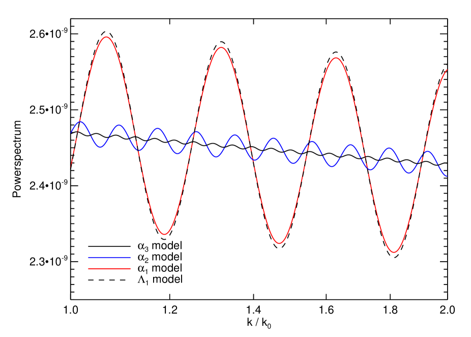
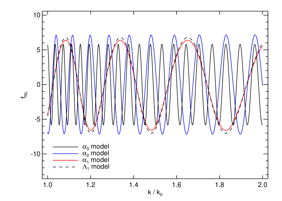
Figure 1: The power- and bispectra for the models in table
Refer to caption
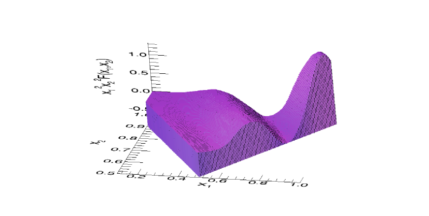
Figure 2: The shape function x12x22F(x1,x2)superscriptsubscript𝑥12superscriptsubscript𝑥22𝐹subscript𝑥1subscript𝑥2x_{1}^{2}x_{2}^{2}F(x_{1},x_{2}) as defined in Eq. (50) for the general αgsubscript𝛼g\alpha_{\textrm{g}} model. Note that by definition F𝐹F is normalised to one for the equilateral form x1=x2=x3=1subscript𝑥1subscript𝑥2subscript𝑥31x_{1}=x_{2}=x_{3}=1, and that we only plot unique triangles, i.e. triangles with x1>x2subscript𝑥1subscript𝑥2x_{1}>x_{2} have been suppressed in the figure for clarity.
Refer to caption
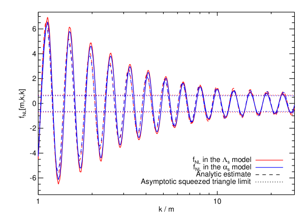
Figure 3: The bispectrum for isosceles triangles for the αssubscript𝛼s\alpha_{\textrm{s}} and ΛssubscriptΛs\Lambda_{\textrm{s}} models as a function of side ratio k/m𝑘𝑚k/m together with the analytic model
Refer to caption
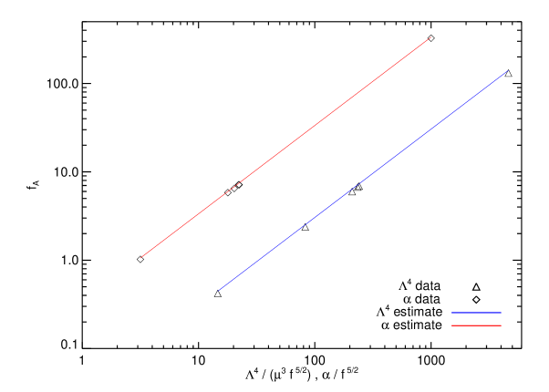
Figure 4: Comparison of the analytic estimates of the amplitudes fAsubscript𝑓𝐴f_{A} of fNLsubscript𝑓NLf_{\mathrm{NL}} to the numerical results.

The power spectra of some of the models is shown in figure 1, and it can be seen that for the given values the oscillations in Pksubscript𝑃𝑘P_{k} are at the per cent to per mill level. For some of the models the wiggles will not even be detected by the Planck satellite [26], while at the same time (see figure 1) they have a significant amount of non-gaussianity. Ref. [26] studied the detectability of ripples due to trans-Planckian effects with Planck or a future cosmic variance limited experiment. In order for ripples to be unambiguously detected their frequency must lie within a range such that there is a number of oscillations in the observable k𝑘k-range and their frequency must be lower than the effective width of the experimental window function. With the frequency, ω𝜔\omega, defined such that P(k)sin(ωlnk)proportional-to𝑃𝑘𝜔𝑘P(k)\propto\sin(\omega\ln k) [26] estimates that 1<w<50superscriptsimilar-to1𝑤superscriptsimilar-to501~{}\mbox{\raisebox{-2.58334pt}{$\stackrel{{\scriptstyle<}}{{\sim}}$}}~{}w~{}\mbox{\raisebox{-2.58334pt}{$\stackrel{{\scriptstyle<}}{{\sim}}$}}~{}50 for it to be detectable. Even if it falls within this range the amplitude must of course also be sufficiently high. At approximately 1σ𝜎\sigma the amplitude, A𝐴A, should be larger than 0.0024 for Planck. Translating to our case we can make the identification ωϕfsimilar-to𝜔subscriptitalic-ϕ𝑓\omega\sim\phi_{*}f and Aδnssimilar-to𝐴𝛿subscript𝑛𝑠A\sim\delta n_{s}. To take an example with the α𝛼\alpha-models: α3,α4,α6subscript𝛼3subscript𝛼4subscript𝛼6\alpha_{3},\alpha_{4},\alpha_{6} have too small amplitude to be detected in P(k)𝑃𝑘P(k). α1subscript𝛼1\alpha_{1} and α2subscript𝛼2\alpha_{2} may be detectable, but α5subscript𝛼5\alpha_{5} has ω50similar-to𝜔50\omega\sim 50 and may have too fast oscillations for a detection. In conclusion, a number of the models with a measurably large non-Gaussianity would not have measurable wiggles in the power spectrum.

We have used our code to probe a rather large range of parameter space, and in figure 4 we show how the analytic estimates for the power spectrum and the bispectrum in the equilateral limit are in excellent agreement with the numerical results. Furthermore, we have also numerically evaluated squeezed triangles (see figure 3), and found a simple functional form Eq. (44) for general isosceles triangles, which agrees at the 5%-level with the numerical result.

Given that the bispectrum in this model is nearly scale invariant, it makes sense to characterise the signal in terms of the shape function [27]

F(x1=k1k3,x2=k2k3,1)=fNL(k1,k2,k3)/fNL(k3,k3,k3)𝐹formulae-sequencesubscript𝑥1subscript𝑘1subscript𝑘3subscript𝑥2subscript𝑘2subscript𝑘31subscript𝑓NLsubscript𝑘1subscript𝑘2subscript𝑘3subscript𝑓NLsubscript𝑘3subscript𝑘3subscript𝑘3F(x_{1}=\frac{k_{1}}{k_{3}},x_{2}=\frac{k_{2}}{k_{3}},1)=f_{\mathrm{NL}}(k_{1},k_{2},k_{3})/f_{\mathrm{NL}}(k_{3},k_{3},k_{3}) (50)

which measures the relative importance of different geometrical configurations compared to the equilateral configuration. In figure 2 it can be seen how the squeezed configurations are suppressed compared to the equilateral configuration. This is also observed in higher derivative models, and is in contrast to local type non-gaussianity from e.g. slow-roll inflation, where the squeezed limit is dominating the shape function [27]. But compared to other models in the literature, this models has the distinct feature of oscillations in fNLsubscript𝑓NLf_{\mathrm{NL}} with an oscillation frequency lnK/ϕfsimilar-toabsent𝐾italic-ϕ𝑓\sim\ln K/\phi f set by the internal parameters of the theory.

5 Conclusions

We have studied in details by numerical and analytical methods the non-Gaussinity generated by a linear single field inflationary potential with superimposed oscillations. This generic form of the potential is an inherent feature of axion monodromy inflation.

The model presents an example of an inflationary model embedded in string theory and can have a very distinct signature on observables. We show that in many cases the main feature of the model is a large non-Gaussianity which is detectable by future experiments such as Planck whereas the impact on the power spectrum is undetectably small. Thus, it appears that the best way to verify this type of models is through a detection of a large bispectrum with the very distinct shape of non-Gaussianity predicted by the model. However, very interestingly it also shares the usual predictions of chaotic inflation type models, i.e. a large tensor-to-scalar ratio and a red spectral index.

Furthermore estimates of the trispectrum in the double-squeezed and in the counter collinear limit shows that non-Gaussianity from the primordial trispectrum could also be detectable by Planck in the present model, although a more careful study of the trispectrum has been left for future studies.

References

References

  • [1] V. Acquaviva, N. Bartolo, S. Matarrese and A. Riotto, Nucl. Phys.  B 667 (2003) 119 [arXiv:astro-ph/0209156].
  • [2] J. M. Maldacena, JHEP 0305 (2003) 013 [arXiv:astro-ph/0210603].
  • [3] D. Seery, J. E. Lidsey and M. S. Sloth, JCAP 0701 (2007) 027 [arXiv:astro-ph/0610210].
  • [4] D. Seery, M. S. Sloth and F. Vernizzi, JCAP 0903 (2009) 018 [arXiv:0811.3934 [astro-ph]].
  • [5] K. Freese, J. A. Frieman and A. V. Olinto, Phys. Rev. Lett.  65, 3233 (1990).
  • [6] N. Arkani-Hamed, H. C. Cheng, P. Creminelli and L. Randall, Phys. Rev. Lett.  90, 221302 (2003) [arXiv:hep-th/0301218].
  • [7] S. Dimopoulos, S. Kachru, J. McGreevy and J. G. Wacker, JCAP 0808 (2008) 003 [arXiv:hep-th/0507205].
  • [8] J. E. Kim, H. P. Nilles and M. Peloso, JCAP 0501 (2005) 005 [arXiv:hep-ph/0409138].
  • [9] N. Kaloper and L. Sorbo, Phys. Rev. Lett.  102 (2009) 121301 [arXiv:0811.1989 [hep-th]].
  • [10] G. G. Ross and G. German, arXiv:0902.4676 [hep-ph].
  • [11] E. Silverstein and A. Westphal, Phys. Rev.  D 78 (2008) 106003 [arXiv:0803.3085 [hep-th]].
  • [12] L. McAllister, E. Silverstein and A. Westphal, arXiv:0808.0706 [hep-th].
  • [13] R. Flauger, L. McAllister, E. Pajer, A. Westphal and G. Xu, arXiv:0907.2916 [hep-th].
  • [14] X. Chen, R. Easther and E. A. Lim, JCAP 0804 (2008) 010 [arXiv:0801.3295 [astro-ph]].
  • [15] A. Curto, E. Martinez-Gonzalez and R. B. Barreiro, arXiv:0902.1523 [astro-ph.CO].
  • [16] O. Rudjord, F. K. Hansen, X. Lan, M. Liguori, D. Marinucci and S. Matarrese, arXiv:0901.3154 [astro-ph.CO].
  • [17] K. M. Smith, L. Senatore and M. Zaldarriaga, arXiv:0901.2572 [astro-ph].
  • [18] E. Komatsu et al. [WMAP Collaboration], Astrophys. J. Suppl.  180, 330 (2009) [arXiv:0803.0547 [astro-ph]].
  • [19] A. P. S. Yadav and B. D. Wandelt, Phys. Rev. Lett.  100, 181301 (2008) [arXiv:0712.1148 [astro-ph]].
  • [20] R. L. Arnowitt, S. Deser and C. W. Misner, [arXiv:gr-qc/0405109]
  • [21] M. S. Sloth, Nucl. Phys.  B 748 (2006) 149 [arXiv:astro-ph/0604488].
  • [22] P. R. Jarnhus and M. S. Sloth, JCAP 0802 (2008) 013 [arXiv:0709.2708 [hep-th]].
  • [23] P. Creminelli and M. Zaldarriaga, JCAP 0410 (2004) 006 [arXiv:astro-ph/0407059].
  • [24] N. Kogo and E. Komatsu, Phys. Rev.  D 73 (2006) 083007 [arXiv:astro-ph/0602099].
  • [25] X. Chen, M.Huang and G. Shiu, Phys. Rev. D74, 121301 (2006) [arXiv:hep-th/0610235]
  • [26] J. Hamann, S. Hannestad, M. S. Sloth and Y. Y. Y. Wong, JCAP 0809 (2008) 015 [arXiv:0807.4528 [astro-ph]].
  • [27] D. Babich, P. Creminelli and M. Zaldarriaga, JCAP 0408, 009 (2004) [arXiv:astro-ph/0405356].