Precision constrained simulation of the Local Universe

Abstract

We use the formalism of constrained Gaussian random fields to compute a precise large scale simulation of the 60$h^{-1}$Mpc volume of our Local Universe. We derive the constraints from the reconstructed peculiar velocities of the 2MASS Redshift Survey. We obtain a correlation of $0.97$ between the log-density field of the dark matter distribution of the simulation and the log-density of observed galaxies of the Local Universe. We achieve a good comparison of the simulated velocity field to the observed velocity field obtained from the galaxy distances of the NBG-3k. At the end, we compare the two-point correlation function of both the 2MRS galaxies and of the dark matter particles of the simulation. We conclude that this method is a very promising technique for exploring the dynamics and structure of the Universe in our neighbourhood.

1 Introduction

We present a new method to re-simulate the large scale structures of the Local Universe to a high precision. Re-simulating the dynamics of the large scale structures in our neighbourhood is an important step to understand the environmental effects that may affect galaxy formation in our part of the Universe and to have better constraints on the potential systematic effects in the observations. Previous attempts, such as Kolatt et al. (1996) and Mathis et al. (2002), used a global constraint of the smoothed density field, which is then transported back in time using Bernoulli-Zel’dovich equation in a 80$h^{-1}$Mpc volume. Narayanan et al. (2001) used PSCz and a perturbative expansion modelling of the evolution of the density field to recover initial conditions in a 50$h^{-1}$Mpc volume. Fontanot et al. (2003) used NOG and PSCz and a semi-Lagrangian reconstruction procedure to obtain the reconstructed displacements in a 60$h^{-1}$Mpc volume. A different approach was followed by Klypin et al. (2003) and Kravtsov et al. (2002) who used Mark III peculiar velocity survey and applied linear theory to obtain pure dynamical constraints, though rather sparse and in a 30$h^{-1}$Mpc volume. Related constrained simulations were then performed in the same manner (e.g Martinez-Vaquero et al., 2007) to study specific local environmental effects. All these reconstructions managed to capture the main large structures but the smaller scales ($\sim$$h^{-1}$Mpc) were not well recovered.

In this work, we use the Monge-Ampère-Kantorovitch (MAK) orbit reconstruction method (Brenier et al., 2003; Mohayaee & Tully, 2005; Lavaux et al., 2008) to recover a dense set of constraints directly in Lagrangian coordinates. We use the catalogue of the reconstructed orbits of the 2MASS Redshift Survey (Huchra, 2000; Huchra et al., 2005) already obtained in Lavaux et al. (2010). We put the constraints object by object using a local adequate Lagrangian smoothing scale which depends on the estimated mass used for the reconstruction procedure.

In Section 2, we present the details of the used methods. In Section 3, we specify the set up of initial conditions from the 2MASS Galaxy Redshift survey. In Section 4 we discuss our results and in Section 5 we conclude.

2 Methods

In this Section, we describe the general methods used to compute and apply the constraints on the initial conditions of the $N$-body simulation. In Section 2.1, we recall the theory of constrained Gaussian realisation. In Section 2.2, we recall the fundamentals of the MAK reconstruction.

2.1 Gaussian constrained realisation

To build the initial conditions of our simulation, we are using a constrained Gaussian realisation algorithm (van de Weygaert & Bertschinger, 1996), derived from the Hoffman-Ribak method (Hoffman & Ribak, 1991). This algorithm allows us to put any linear constraint of a Gaussian random density field, which corresponds to the initial condition of an $N$-body simulation. We give here a summary of the steps of the algorithm. We first compute the variance matrix $V_{i,j}$ of the kernel of the constraints:

$$V_{i,j}=\int\text{d}^{3}{\bf k}P(k)\hat{K}^{*}_{i}({\bf k})\hat{K}_{j}({\bf k})$$ (1)

with $K_{i}({\bf k})$ the kernel window function given in appendix F of van de Weygaert & Bertschinger (1996). We build the Fourier transform $\hat{\delta}_{\text{r}}({\bf k})$ of a Gaussian random field and then compute the constrained realisation

$$\hat{\delta}({\bf k})=\hat{\delta}_{\text{r}}({\bf k})+\sum^{N_{\text{c}}}_{i,j=1}V^{-1}_{i,j}(c_{j}-c^{\text{m}}_{j})K_{i}({\bf k})$$ (2)

with $c_{j}$ the value of the constraint, $N_{\text{c}}$ the number of constraints and

$$c^{\text{m}}_{j}=\int\text{d}^{3}{\bf k}K_{j}^{*}({\bf k})\hat{\delta}_{\text{r}}({\bf k}).$$ (3)

After the inverse Fourier transform, the field $\delta({\bf r})$ satisfies both the constraints and the power spectrum. Practically all the integrals are computed on the lattice of the finite discrete Fourier coefficients.

The type and number of constraints is left free but must be linearly obtained from the density field $\delta$. For example, one may put constraints on the local shape of the density field and its peculiar velocity at the same time. In this case, we have thus 10 constraints for the local shape of the density field, which corresponds to its value, its first and second derivatives. Additionally, we have 3 constraints for the peculiar velocity. Once the constraints have been put on the density, the rest of the density field is generated to match a given cosmological power spectrum such that the statistics of the final initial conditions are statistically correct. We note that this constrained realisation algorithm is fundamentally in Lagrangian coordinates to set up initial conditions for the dynamics of matter particles. This is particularly true for the choice of the size of the filter in the kernel $K_{i}$, which must be understood in terms of Lagrangian coordinates.

We implemented such an algorithm in a MPI parallel environment. This code is capable of handling an arbitrary number of Gaussian constraints of any size. The memory and processor load is shared evenly among all nodes of the cluster, making this code scalable on a MPI cluster of computer.

2.2 The MAK reconstruction

We propose to use the results obtained through the Monge-Ampère-Kantorovitch (MAK) reconstruction to find the constraints to put on the initial conditions of an $N$-body simulation. The MAK reconstruction is a non-linear scheme of recovering the peculiar velocity field from an evolved non-linear density field. It assumes that the dynamics has not suffered shell crossing. In that case, it has been shown (Brenier et al., 2003) that it is possible to uniquely reconstruct the trajectories of the particles from initial to present time. Practically, the reconstruction corresponds to finding the mapping $\sigma$ which minimises the quantity (Brenier et al., 2003)

$$S_{\sigma}=\sum_{i=1}^{N}({\bf q}_{\sigma(i)}-{\bf x}_{i})^{2},$$ (4)

where the $\{{\bf x}_{i}\}$ are the Eulerian coordinates of equal mass particles composing the present day non-linear density field, $\{{\bf q}_{j}\}$ are the homogeneously distributed Lagrangian coordinates of this same distribution. This method is thus purely Lagrangian. Additionally, full mass conservation is hard encoded in the method, removing the singularities that are present in linear theory in the neighbourhood of large mass concentration. The assumption that no-shell crossing occurs is of course limited to larger scales, typically a few megaparsecs, where structures are still in the Lagrangian perturbative regime, called the Zel’dovich approximation. This modelling of the dynamics is sufficient for our purpose which is to compute initial conditions compatible with observations on large scales.

To handle redshift space distortions, we use the Zel’dovich approximation to predict the peculiar velocities of particles at the moment of the reconstruction. The modified action has been shown to work well on large scales for the reconstruction of peculiar velocities (Mohayaee & Tully, 2005; Lavaux et al., 2010).

This method is particularly well suited to work in conjunction with the Hoffman-Ribak method as we derive all quantities in Lagrangian coordinates.

3 Computing initial conditions

In this section, we describe the methodology used to go from the original 2MRS data-set to the finished initial conditions of the $N$-body simulation. Section 3.1 describes the data-set. Section 3.2 describes how the constraints were applied to the random Gaussian field. At the end, Section 3.3 gives the details of the setup of the initial conditions, in particular the choice of the background cosmology.

3.1 Dataset

To get better constraints for the simulation of the Local Universe, we have used the 2MASS redshift survey, which has the advantage of being full-sky, compared to other surveys, while being complete up to $\sim$60-80$h^{-1}$Mpc. To derive the mass distribution for the orbit reconstruction, we assume a constant Mass-to-Light ratio. This hypothesis has already given successful results on the comparison between reconstructed and observed peculiar velocities using this catalogue (Lavaux et al., 2010).

We use the mass splitter algorithm given in Appendix A of Lavaux et al. (2008). The algorithm looks for the optimal equal mass splitting given that we have a fixed number of mass elements and that the relative error between the splitted and the true mass must be as low as possible. After the reconstruction of the displacements of the equal mass particles, the global displacement of each of the groups of galaxies is computed by a simple average of the displacements of the particles representing this group.

To mitigate boundary effects in the inner part of the reconstruction volume, we use a 100$h^{-1}$Mpc deep reconstruction, padded with an homogeneous distribution of particles, as specified in Lavaux et al. (2008), and have extracted the objects within 60$h^{-1}$Mpc for the Local Group.

We have not used all of the objects for constraining the Gaussian realisation as it would have yielded a 19913$\times$19913 matrix to compute and invert. This would be expensive to compute exactly, and additionally inversion would probably need to be regularised. Instead, we limit ourselves to constrain the reconstructed peculiar velocities of the bigger objects. We now describe the methodology used to constrain the Gaussian realisation.

3.2 Constraining initial conditions

We constrain the realisation within 60$h^{-1}$Mpc of the centre of the box, which corresponds to our mock observer, using the reconstructed velocities obtained from the MAK reconstruction. This reconstruction has been shown to recover with precision the linear regime from an evolved non-linear density field (Mohayaee et al., 2006; Lavaux et al., 2008). We use the reconstructed 3D displacement field in Lagrangian coordinates to constrain the motion of matter. We choose an isotropic Gaussian smoothing window whose radius, $R_{i}$, is determined by the mass of the considered object $i$ in the catalogue and is given by:

$$R_{i}=\frac{1}{\sqrt{5}}\left(\frac{3M_{i}}{4\pi\bar{\rho}}\right)^{1/3}.$$ (5)

We add a $1/\sqrt{5}$ to match the Gaussian filter scale to a top hat filter scale to second order in Fourier space. The top hat filter is a good indicator of the filtering scale as the peculiar velocities are computed by doing a simple average of all displacements of the particles of a given group of galaxies when computing the total displacement of this group. We neglect the impact of the actual shape of the Lagrangian patch of the considered objects. To avoid having too many constraints, we enforce that the constraint should at least have a Lagrangian radius $R_{i}\geq 1.5$$h^{-1}$Mpc. This corresponds to considering only the peculiar velocities of groups of a mass greater than $\sim 4\times 10^{12}$ M_⊙. This allows us to reduce the size of the matrix to 3942$\times$3942. In doing so we make use of the sensitivity of the peculiar velocities to large scale power in order to reduce the computational complexity while keeping the results intact. Indeed, for a typical $\Lambda$CDM cosmology, the velocity field is correlated at $\sim 90\%$ for distances less than $\sim 8$$h^{-1}$Mpc. Consequently, we do not add much information by increasing the number density of constraints. Instead, we may even decrease the numerical stability of the method, which relies on a large matrix inversion. We discuss the impact of keeping only one fourth of these constraints at the end of Section 4.3. We expect that increasing the density of constraints should not change our results significantly. We include in Appendix A a comparison between the simulated velocity field and the original constraints.

3.3 Initial condition setup

We use a Bardeen et al. (1986) power spectrum with $n_{s}=1$, $\Omega_{\text{m}}=0.258$, $\Omega_{\Lambda}=0.742$, $H=72$ km.s^-1.Mpc^-1, $\sigma_{8}=0.77$. The time complexity increases with the number of constraints $N_{\text{C}}$ as $O(N_{\text{C}}\times N_{\text{g}})$, with $N_{\text{g}}$ the mesh size for generating initial conditions. We choose a mesh of $N_{\text{g}}=256^{3}$ particles, sampling a box of side $L=200$$h^{-1}$Mpc for generating the constrained initial conditions. This allows us to shape the white noise at a resolution of $\sim$1$h^{-1}$Mpc while keeping the time complexity low. At the end, we constrain 1,314 positions in a $\sim$60$h^{-1}$Mpc volume in Lagrangian coordinates, which corresponds to 3,942 constraints. The computation of the correlation matrix of the constraints at this resolution took a little less than a week on 128 processors on the Mercury cluster at NCSA.

4 Results

Figure 1: Observed vs simulated sky-maps – Left column: Aitoff projection of the galaxies of the Two-Micron-All-Sky Redshift survey in different redshift slices, as indicated above the panel. Right column: Aitoff projected mass density in different redshift slices of the simulation, centred on the mock observer at the centre of the simulation. The contrast of the different slices have been adjusted for the distance of each slices.

Figure 1: continued

In this section, we detail the results of the constrained simulation. We used the $N$-body simulation code RAMSES (Teyssier, 2002) to evolve the initial condition that are specified in Section 3.3. The background metric is chosen to be a standard $\Lambda$CDM cosmology with parameters $\Omega_{\text{m}}=0.258$, $\Omega_{\Lambda}=0.742$, $H_{0}=72$ km.s^-1.Mpc^-1. We limit the number of refinement of the AMR grid to seven, this corresponds to soften the gravitational field on the scale of $\sim 6h^{-1}$kpc, which is the size of one element of the mesh. We first look qualitatively at the sky-maps of the distribution of the dark matter. We then check the adequacy of the simulated velocity field to the observed velocity field within a volume of 3,000 km.s^-1. Finally, we compare quantitatively the simulated density field to the observed galaxy density field: by direct comparison and through the two point correlation function.

4.1 Sky-maps

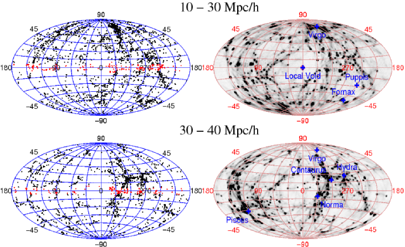
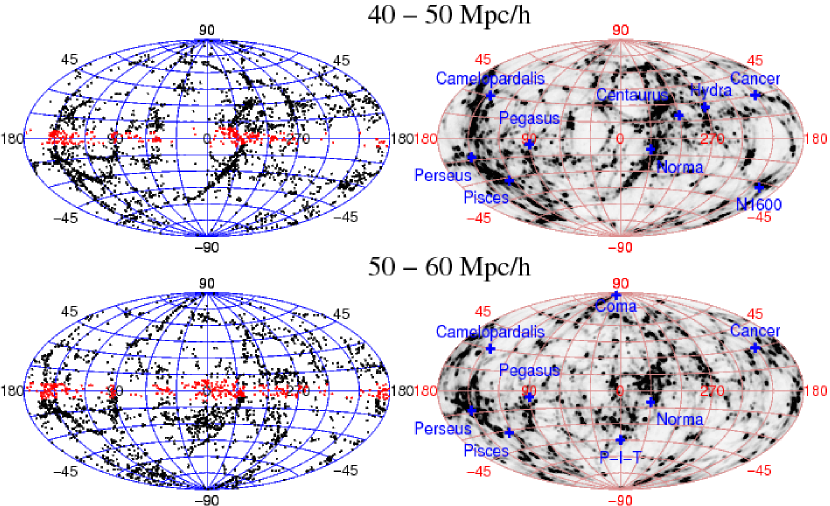
In the left column of Figure 1, we represent the position of galaxies by redshift slices on an Aitoff projection of the real sky. In the right column, we represent the projected mass density of the simulation in these same slices. The colour contrast is corrected such that the maximum value represented in these sky map is proportional to $1/2(d_{i+1}-d_{i})(d_{i}+d_{i+1})^{2}$. This ensures that clusters are not excessively dominating the map at larger distances compared to maps of the structures at smaller distances.

The visual comparison of the structures seen in the 2MASS Redshift Survey and in the simulation looks qualitatively in agreement. We reproduce nearly all the filamentary structure of the Local Universe. We now look at the details of the structures in each of the slices.

In the $10-30$$h^{-1}$Mpc slice, Virgo is at its right place near the North Galactic Pole. At the south pole, there is a significant dark matter concentration that is probably linked to a set of galaxies present in the 2MRS in the same slice. We correctly recover the Fornax cluster at $(l,b)\simeq(236,53)$ with the Puppis cluster. We see that the Local Void area is totally empty as it is expected from recent peculiar velocity analysis (Tully et al., 2008). This void unfortunately corresponds to a region that is currently obscured by the galactic bulge of our galaxy. It is present in the reconstructed velocity field because we assume that the galaxies above and below the galactic bulge were a fair representation of what is happening in the direction of the bulge. As the number of galaxies is very low, it happens that we have introduced a Local Void of the right size, as expected from peculiar velocities. This void now appears in the simulation. Additionally, we recover all the observed filaments. In the right panel, we see the first tip of the Pisces cluster at $(l,b)\sim(150,-30)$. We note a filament that goes from this cluster to the Great Attractor region in the Hercules sector. This filament is lightly visible in the distribution of galaxies on the left panel.

In the $30-40$$h^{-1}$Mpc slice, the galaxy distribution features are almost completely reproduced in the dark matter density field of the $N$-body simulation. The first tip of the Pisces cluster appear in that slice, even though it should be mostly placed in the the 50$h^{-1}$Mpc region. In the Great Attractor direction, $(l,b)\sim(300,15)$, we see that the simulation follows very precisely the distribution of galaxies on the left. The two concentrations of galaxies in the middle of the sky projection correspond to the Hydra-Centaurus supercluster, as highlighted in the right panel. The filaments are correctly visually interconnected according to the galaxy distribution. The Local Void is still present in this slice.

So far, the number of galaxies introduced to fill the Zone of Avoidance was small. In the $40-50$$h^{-1}$Mpc slice, this number increases. We recover all marked structures of the right panel of this slice. We also recover the structures introduced by the filling of the Zone of Avoidance. For example, the “S” shape in the direction $(l,b)\sim(300,0)$ is recovered in the distribution of dark matter. So, the constrained initial condition are working even better than expected in that respect, even though this shape may be an artificial construction due to the Zone-of-Avoidance filling using mirrored galaxies.

The galaxy distribution in the $50-60$$h^{-1}$Mpc slice is totally reproduced in the dark matter density field of the simulation.

4.2 Velocity fields

Figure 2: Simulated peculiar velocities along the line-of-sight vs. observed peculiar velocities – We represent here the direct comparison of the simulated velocity field against the observed velocity field (line-of-sight component) within the 30$h^{-1}$Mpc volume. We subtracted the 30$h^{-1}$Mpc bulk flow in the two cases. The filled contours corresponds to 50% (black), 68% (dark grey), 95% (grey), 99% (light grey) of the 30$h^{-1}$Mpc volume. Both velocity fields were adaptively smoothed with a spline of radius in the range $[2.5;13]$$h^{-1}$Mpc, with a median of 7$h^{-1}$Mpc.

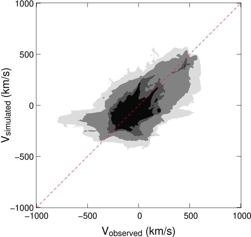
In Figure 2, we compare quantitatively the simulated line-of-sight component velocity field to the observed line-of-sight component of the velocity field. For obtaining the observed velocity field we used the extended NBG-3k catalog (Tully et al., 2008). The distance were matched to the group of galaxies of the 2MASS Redshift Survey galaxies so that 726 groups receive a distance (Crook et al., 2007; Lavaux et al., 2010). We did an equivalent treatment for the simulation. We first grouped the particles according to a Friend-Of-Friend algorithm with a linking length of $0.2\bar{n}^{-1/3}$, with $\bar{n}$ the mean particle density of the simulation (Efstathiou et al., 1988). We applied a threshold of having a minimum of 8 particles. This grouping helps at reducing Finger-Of-God phenomena while keeping other redshift distortion effects.

The two velocity fields are computed in redshift space to avoid systematic effects (e.g. Lynden-Bell et al., 1988; Dekel et al., 1990). Moreover, to avoid being contaminated by Finger-of-god effects, we first computed groups using a Friend-Of-Friend algorithm in the simulation (linking length equal to 0.2 the mean inter-particle length). We also used the distance to grouped galaxies obtained from the anisotropic Friend-Of-Friend that we used to make the groups of galaxies in the 2MASS Redshift Survey. This anisotropic Friend-of-Friend is described in Huchra & Geller (1982); Crook et al. (2007); Lavaux et al. (2010).

The two velocity fields agree well with each other, although there is a large scatter. This scatter has at least three origins: the modelling error of the dynamics in the reconstruction of the orbits of the galaxies of the 2MRS, the modelling error of the Zel’dovich transport when applying the constraints coming from reconstruction and the measurement errors on the observed velocity field.

4.3 Density field

Figure 3: Correlation of the density field of the simulation to the density field of the 2MRS catalogue – We have extracted a volume limited sample of 60$h^{-1}$Mpc from the 2MRS and the equivalent volume from the simulation. The density fields are both smoothed to 3.5$h^{-1}$Mpc with a Gaussian kernel.

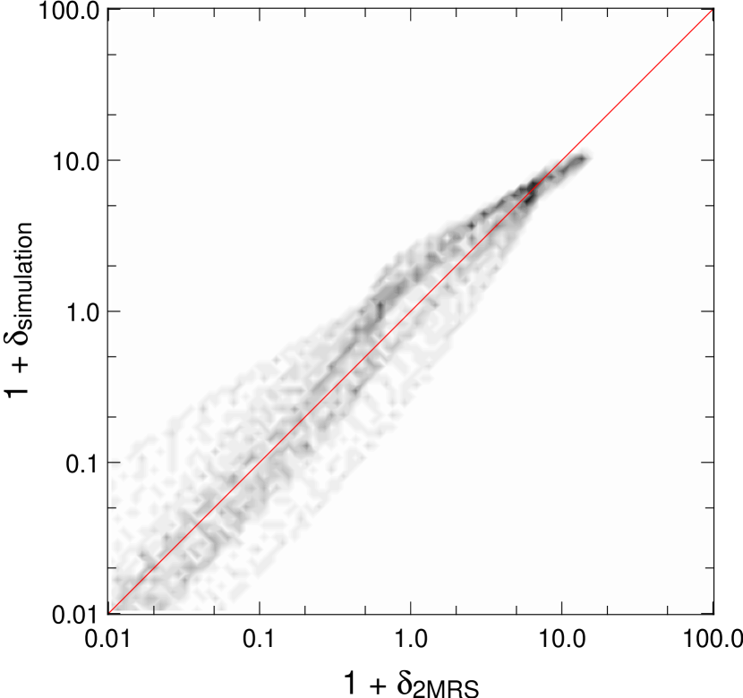
In Fig. 3, we show the correlation of the density field of the simulation and of the 2MRS galaxy number, smoothed to 3.5$h^{-1}$Mpc with a Gaussian kernel. We define the correlation coefficient as the ratio:

$$r=\frac{\langle\log(\rho_{\text{sim}}/\bar{\rho_{\text{sim}}})\log(\rho_{\text{obs}}/\bar{\rho_{\text{obs}}})\rangle}{\sqrt{\langle(\text{log}(\rho_{\text{sim}}/\bar{\rho_{\text{sim}}}))^{2}\rangle\langle(\text{log}(\rho_{\text{obs}}/\bar{\rho_{\text{obs}}}))^{2}\rangle}},$$ (6)

with $\rho_{\text{sim}}$ the smoothed density field of the simulation, $\rho_{\text{obs}}$ the smoothed galaxy number density field in a volume limited sample 2MASS Redshift Survey. The correlation coefficient of the logarithm of the density field is 0.97. This correlation is not perfect. On the high end, we see that the main alignment of the scatter distribution is not strictly following the red diagonal. This could be an effect of the galaxy bias at that scale. Reducing the number of constraints on the initial condition from 3,942 to $\sim$1,000, either by selecting more massive objects or by randomly picking up one constraint of four, leads to a decrease of the correlation of the two density fields to $0.92$. Additionally, we see a significant increase in the scatter in the high density region, the low density being apparently unaffected. The scatter in the simulated velocity field remains unaffected by this change.

4.4 Two point correlation function

Figure 4: Two point correlation function of the galaxies and of the dark matter in the simulation – We have computed the two-point correlation function of the dark matter particles of the simulation (red) and of the galaxies of the 2MASS Redshift Survey (black) for the volume limited sample of 60$h^{-1}$Mpc of volume. We represented the ratio $b^{2}=\xi_{\text{2MRS}}/\xi_{\text{simulation}}$ in the inset plot. The error bars are estimated using a Jackknife test on 1,000 sub-volumes with 1,000 different realisations of the sampling noise of the volume.

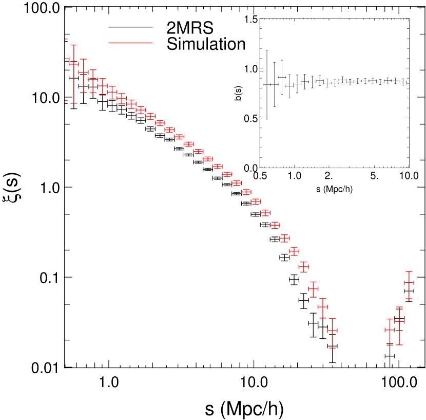
Another quantitative comparison between observations and simulation is given by the two point correlation function. Comparing the two point functions given by the dark matter distribution of the re-simulation of our Local Universe and the actual two point function of the galaxies of our Universe may allow to have a better understanding of the galaxy distribution bias by direct measurement. We propose here a simple test to estimate the scale dependent bias in our specific part of the Universe by taking the ratio of these two functions.

We use the estimator of Landy & Szalay (1993) to compute the correlation function within a 60$h^{-1}$Mpc volume:

$$\xi(s)=\frac{DD(s)-2DR(s)+RR(s)}{RR(s)},$$ (7)

with $s$ the amplitude of the redshift separation. We have built a volume limited sample of the 2MRS such that it is complete up to a distance of 60$h^{-1}$Mpc from the observer, which corresponds to keeping 5,472 galaxies. In this test, we are not sensitive to cosmic variance effects as we are looking at the same part of the Universe both in the simulation and in the observations. So, the error bars on our correlation function should only reflect the sampling errors. To estimate these errors, we have sub-divided the 60$h^{-1}$Mpc volume into 1,000 sub-volumes and performed a Jackknife test by computing the correlation function on the whole 60$h^{-1}$Mpc except the concerned volume. For each of the computation of the correlation function, we have used a different realisation of the sampling noise used to compute $RR$ and $DR$. This generated 1,000 correlation functions compatible with the data.

We have computed the correlation function of the simulation in exactly the same way. We have first extracted randomly 5,472 particles, and we have applied the same cuts in volume as for the catalogue, including the Zone-of-Avoidance effect.

The results are given in Fig. 4. The central point of the correlation function corresponds to the average of all the obtained correlation function by the Jackknife test and the Poisson sampling test. The vertical error bars reflect the standard deviation of $\xi(s)$ according to its average. The horizontal error bar gives the size of the bin.

We see that the two correlation function are closely following each other except on the smaller scales. This is expected as we implicitly assumed in the reconstruction that galaxies are fair tracers on large scales. We note that, in our case, the value of the bias for the galaxies of the 2MRS seems to be $b=0.87\pm 0.03$. However, this result is probably systematically affected by the particular value of $\sigma_{8}$ for the realisation of the large scale mode of the simulation, which are more compatible with $\sigma_{8}=0.83$ instead of $\sigma_{8}=0.77$. This can introduce a small bias of the order of $0.93$, which corresponds to what we observe here. Additionally, the fair comparison between the simulated velocity field and the observed velocity field (Fig. 2) reinforces this result as the velocity field is sensitive to the total matter distribution, even though we used a constant mass-to-luminosity ratio to derive the mass of each galaxy to reconstruct their orbits.

5 Conclusion

We have implemented a new method to re-simulate the Local Universe with a standard $N$-body simulation code from the 2MRS catalogue of galaxies. This method allows us to reproduce in many details the Large-scale structures of the Local Universe up to 60$h^{-1}$Mpc and to a precision of a few megaparsecs. This method is easily applicable to larger volumes and surveys. We illustrate the quality of the simulated volume by direct comparison within a 30$h^{-1}$Mpc volume of the simulated velocity field to the observed velocity field. Furthermore, we highlight a direct application of this simulation by the joint measurement of the two point correlation function in the simulation and in the actual observations of the positions of the galaxies of the 2MRS.

This method opens us the possibility of studying quantitatively both larger and smaller scales for our Local Universe. On small scales, such a simulation would allow to run a simulation of the Local Group including environmental effects. On large scales, we would like to extend this work to the quantitative comparison between CMB data and Large Scale structure data, with the major advantage, compared to earlier attempts, of taking into account non-linear dynamics and clustering. Along with semi-analytic modelling of galaxy formation, it is possible to build a non-statistical simulation of the galaxies in our sky, which would enable us to make a direct quantitative comparison with observations.

Appendix A Comparison of the reconstructed to the simulated velocity field

Figure 5: Simulated velocity field vs. original reconstructed velocity field – We represent here a quantitative comparison of the originally reconstructed velocity field, which was used to constrain the initial conditions, against the final simulated velocity field. We used the same colour convention and the same smoothing procedure as in Figure 2.

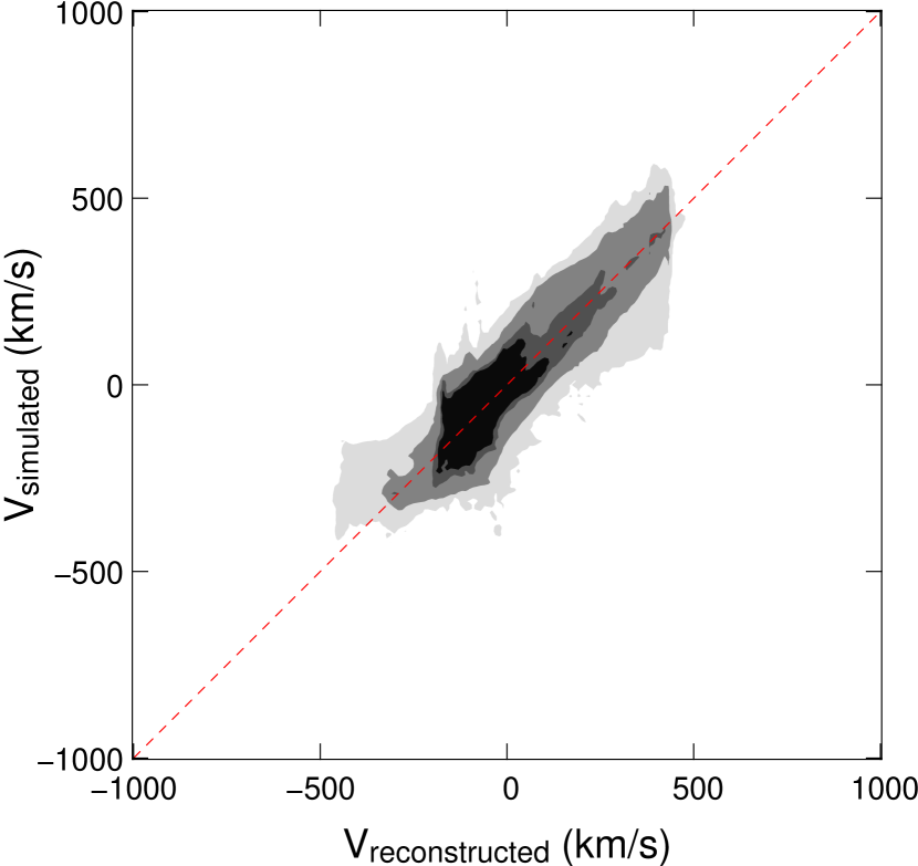
We represent in Figure 5 a comparison of the original reconstructed velocity field, used to derive the constraints on the initial conditions, to the simulated velocity field, obtained by evolving the initial condition using an $N$-body simulation. We note that the two fields are fairly equal up to some scatter that is probably due to small scale clustering, which is not modelled by the MAK reconstruction, and the imperfections of the Zel’dovich approximation, used to derive the velocity field constraints.

References

- Bardeen et al. (1986) Bardeen J. M., Bond J. R., Kaiser N., Szalay A. S., 1986, ApJ, 304, 15
- Brenier et al. (2003) Brenier Y., Frisch U., Hénon M., Loeper G., Matarrese S., Mohayaee R., Sobolevskiĭ A., 2003, MNRAS, 346, 501, arXiv:astro-ph/0304214
- Crook et al. (2007) Crook A. C., Huchra J. P., Martimbeau N., Masters K. L., Jarrett T., Macri L. M., 2007, ApJ, 655, 790, arXiv:astro-ph/0610732
- Dekel et al. (1990) Dekel A., Bertschinger E., Faber S. M., 1990, ApJ, 364, 349
- Efstathiou et al. (1988) Efstathiou G., Frenk C. S., White S. D. M., Davis M., 1988, MNRAS, 235, 715
- Fontanot et al. (2003) Fontanot F., Monaco P., Borgani S., 2003, MNRAS, 341, 692, arXiv:astro-ph/0301601
- Hoffman & Ribak (1991) Hoffman Y., Ribak E., 1991, ApJL, 380, L5
- Huchra et al. (2005) Huchra J., Martimbeau N., Jarrett T., Cutri R., et al. 2005, in Colless M., Staveley-Smith L., Stathakis R. A., eds, Maps of the Cosmos Vol. 216 of IAU Symposium, 2MASS and the Nearby Universe. p. 170
- Huchra (2000) Huchra J. P., 2000, in Courteau S., Willick J., eds, Cosmic Flows Workshop Vol. 201 of Astronomical Society of the Pacific Conference Series, The 2MASS Redshift Survey. p. 96
- Huchra & Geller (1982) Huchra J. P., Geller M. J., 1982, ApJ, 257, 423
- Klypin et al. (2003) Klypin A., Hoffman Y., Kravtsov A. V., Gottlöber S., 2003, ApJ, 596, 19, arXiv:astro-ph/0107104
- Kolatt et al. (1996) Kolatt T., Dekel A., Ganon G., Willick J. A., 1996, ApJ, 458, 419, arXiv:astro-ph/9509066
- Kravtsov et al. (2002) Kravtsov A. V., Klypin A., Hoffman Y., 2002, ApJ, 571, 563, arXiv:astro-ph/0109077
- Landy & Szalay (1993) Landy S. D., Szalay A. S., 1993, ApJ, 412, 64
- Lavaux et al. (2008) Lavaux G., Mohayaee R., Colombi S., Tully R. B., Bernardeau F., Silk J., 2008, MNRAS, 383, 1292, arXiv:0707.3483
- Lavaux et al. (2010) Lavaux G., Tully R. B., Mohayaee R., Colombi S., 2010, ApJ, 709, 483, arXiv:0810.3658
- Lynden-Bell et al. (1988) Lynden-Bell D., Faber S. M., Burstein D., Davies R. L., Dressler A., Terlevich R. J., Wegner G., 1988, ApJ, 326, 19
- Martinez-Vaquero et al. (2007) Martinez-Vaquero L. A., Yepes G., Hoffman Y., 2007, MNRAS, 378, 1601, arXiv:0704.3385
- Mathis et al. (2002) Mathis H., Lemson G., Springel V., Kauffmann G., White S. D. M., Eldar A., Dekel A., 2002, MNRAS, 333, 739, arXiv:astro-ph/0111099
- Mohayaee et al. (2006) Mohayaee R., Mathis H., Colombi S., Silk J., 2006, MNRAS, 365, 939, arXiv:astro-ph/0501217
- Mohayaee & Tully (2005) Mohayaee R., Tully R. B., 2005, ApJL, 635, L113, arXiv:astro-ph/0509313
- Narayanan et al. (2001) Narayanan V. K., Weinberg D. H., Branchini E., Frenk C. S., Maddox S., Oliver S., Rowan-Robinson M., Saunders W., 2001, ApJS, 136, 1, arXiv:astro-ph/9910229
- Teyssier (2002) Teyssier R., 2002, A&A, 385, 337, arXiv:astro-ph/0111367
- Tully et al. (2008) Tully R. B., Shaya E. J., Karachentsev I. D., Courtois H. M., Kocevski D. D., Rizzi L., Peel A., 2008, ApJ, 676, 184, arXiv:0705.4139
- van de Weygaert & Bertschinger (1996) van de Weygaert R., Bertschinger E., 1996, MNRAS, 281, 84, arXiv:astro-ph/9507024