Boolean Models of Bistable Biological Systems

Abstract

This paper presents an algorithm for approximating certain types of dynamical systems given by a system of ordinary delay differential equations by a Boolean network model. Often Boolean models are much simpler to understand than complex differential equations models. The motivation for this work comes from mathematical systems biology. While Boolean mechanisms do not provide information about exact concentration rates or time scales, they are often sufficient to capture steady states and other key dynamics. Due to their intuitive nature, such models are very appealing to researchers in the life sciences. This paper is focused on dynamical systems that exhibit bistability and are described by delay equations. It is shown that if a certain motif including a feedback loop is present in the wiring diagram of the system, the Boolean model captures the bistability of molecular switches. The method is applied to two examples from biology, the lac operon and the phage $\lambda$ lysis/lysogeny switch.

Franziska Hinkelmann^a,b,c and Reinhard Laubenbacher^b,c

^aInterdisciplinary Center for Applied Mathematics, Virginia Polytechnic Institute and State University,

Blacksburg, VA 24061-0531, USA

^bDepartment of Mathematics, Virginia Polytechnic Institute and State University,

Blacksburg, VA 24061-0123, USA

^cVirginia Bioinformatics Institute, Virginia Polytechnic Institute and State University,

Blacksburg, VA 24061-0477, USA

1 Introduction

Since the discovery of the first gene regulatory network, the lactose metabolism network in the bacterium E. Coli by Jacob Monod, [8], such networks have been modeled extensively, traditionally with differential equations. But other modeling techniques like Boolean networks [1], stochastic models [15], Petri nets, or Bayesian networks [7] have also been used successfully. Work by Kauffman in 1969 [9] suggested that gene networks behave like Boolean switching nets and therefore Boolean networks are suitable to model them. Using a Boolean network model, it has been shown, for instance, that in some cases the network topology and the logic of the interactions among the different molecular species is sufficient to determine the qualitative dynamics of the network, without taking into account the detailed kinetics [1]. In cases where not enough information about the kinetic parameters is available to build a detailed continuous model, one often still has enough information to build a Boolean network model which can provide important information.

The purpose of this paper is to show for a particular family of continuous models that they can be approximated by a Boolean network model that retains the key information about model dynamics. Our intent is to demonstrate that Boolean models can be used to study a variety of structural and dynamic features of biological and other systems that have traditionally been modeled using continuous models. They have the added advantage that they are intuitive and do not require much mathematical background. This makes them particularly suitable for use in the life sciences. The focus of this paper is on two features: bistability and time delays. We give a general algorithm how to approximate a dynamical system given by a system of ordinary delay differential equations by a Boolean network model and validate it with two well-known examples from systems biology. The relation between discrete and continuous models has been examined before, e.g., [6] describes how a logical network can be used to create the analogous differential equations. Other methods allow to systematically create a continuous model from a discrete dynamical system [11], or to reduce the model space by using a finite state machine [4]. We briefly review the main concepts related to Boolean network models.

1.1 Introduction to Boolean Models

We use a time discrete deterministic Boolean network with synchronous update. In a Boolean model, a variable can only be in the “on” (1) or “off” (0) state. In systems biology applications, each variable typically corresponds to a molecular entity, e.g., the concentration of a gene product such as mRNA or proteins. A Boolean network of $n$ variables consists of an update function $f=(f_{1},\ldots,f_{n}):\mathbb{F}_{2}^{n}\rightarrow\mathbb{F}_{2}^{n}$, also called a transition function. The dynamics of the system are generated deterministically by iteration of the transition function $f$. It can be visualized by its phase space, which shows all possible states and their transitions. A cycle in the phase space is called a limit cycle; if it has length one, a fixed point. Fixed points of a discrete system are the equivalent to steady states of a continuous system.

In the dependency graph, also referred to as wiring diagram, each variable is a vertex and an edge from variable $x_{i}$ to $x_{j}$ is drawn if $x_{i}$ shows up in the local transition function $f_{j}$. A directed cycle in the dependency graph is called a feedback loop.

Example

Consider the following Boolean network with three variables:

$$f_{1} =((\neg x_{1})\wedge x_{3})$$

$$f_{2} =(x_{1}\wedge x_{3})$$

$$f_{3} =((x_{1}\wedge x_{2})\vee x_{3}).$$

The phase space of this function is depicted in Fig 1. The network has a limit cycle of length two because the state $(1\ 0\ 1)$ transitions into $(0\ 1\ 1)$, which turns back to $(1\ 0\ 1)$. It also includes the fixed point $(0\ 0\ 0)$.

Figure 1: Phase space of $f=(\neg x_{1}\wedge x_{3},x_{1}\wedge x_{3},(x_{1}\wedge x_{2})\vee x_{3})$

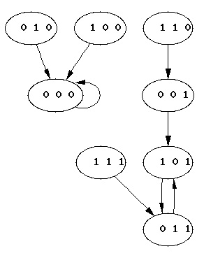
Discrete Visualizer of Dynamics (DVD tool) [10] was used to create the phase space. It calculates the number and length of limit cycles and fixed points, as well as the trajectories from any initial state. It also generates a graph of the phase space along with the dependency graph.

2 Approximation by Discrete Models

We begin by describing several relevant features of biochemical networks that a model needs to capture and describe in each case how this is done in the Boolean network case. We use lower case letters for continuous variables and upper case letters for discrete ones.

2.0.1 Dilution and Degradation

It is common in biochemical networks that the concentration of a substance $X$ decreases with time because of dilution and degradation. In a differential equations model this is usually accounted for with a negative degradation term:

$$\frac{dx}{dt}=\cdots-\gamma x.$$

In the discrete model, for simplicity it is assumed that the degradation rate for a substance is either vanishingly small and can therefore be ignored, or the substance is degraded below the threshold for discretization after two discrete timesteps.

To model the decrease of concentration of a substance by dilution and degradation, which is modeled in the continuous case by a negative degradation term for $x$, a new variable $X_{\text{old}}$ is introduced. If $X_{\text{old}}$ is “on,” then any quantity of $X$ that is available has already been reduced once by dilution and degradation, and if no new substrate is produced, $X$ will be “off” in the next time step.

2.0.2 Time Delay

In gene regulatory networks, time delays are often caused by transcription and translation. Dependence of a variable $x$ on the concentration of a substance $y$ time $\tau$ ago can be described with a delay differential equations model

$$\frac{d}{dt}x(t)=\ldots\ y(t-\tau)\ \ldots$$

In a time discrete model, further variables are needed to model this delay. One has to choose the length $\overline{t}$ of a discrete timestep. If the delay $\tau=\overline{t}$, then $X$ is chosen to depend on $Y_{1}$ and $Y_{1}$ depends on $Y$.

$$f_{X} =\ldots Y_{1}\ldots$$

$$f_{Y} =\ldots$$

$$f_{Y1} =Y$$

If $\tau>\overline{t}$, additional variables have to be introduced.

2.0.3 Distinguishing between Low, Medium, and High Concentrations

To differentiate between three states for a variable $X$ in a Boolean system, a second variable $X_{\text{high}}$ is introduced. By doing so one can make a distinction between low, medium, and high concentration of $X$: if $X$ is on, the concentration is a least medium, whereas $X_{\text{high}}$ is only on, if the concentration is high.

2.0.4 Bistability

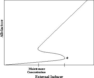
If previous experiments or computations have shown that the system exhibits bistable behavior depending on the concentration of a stimulus $X$, it is necessary to distinguish in the model between different concentrations of $X$: the concentrations for which there is a unique steady state for the system and for which there are multiple possible steady states. Without this distinction, a Boolean model could not capture bistability. In the lac operon, a medium allolactose concentration leads to bistability, therefore the discrete model must differentiate between low, medium, and high concentration of allolactose.

Figure 2: Necessary motif in dependency graph for bistability

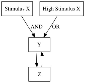
The stimulus $X$ is the parameter that drives a system in and out of the bistable region; within the bistable region the previous state determines the resulting steady state. The stimulus acts on one or more variables. Usually $X_{\text{high}}$ is part of an OR statement in the transition function (if the stimulus is present in high concentration, it should overrule everything and turn the system on), whereas $X$ is part of an AND statement (under its presence other factors might prevent the system from turning on). The state of $Z$ (this could be a set of variables or a single variable) indicates whether the system was in a preinduced state before the stimulus concentration was changed or not, depending on the input from $Z$:

$$Y=(Z\wedge X)\vee X_{\text{high}}.$$

To assure that $Z$ reflects whether the system was preinduced, $Z$ needs to receive input from $Y$. This leads to a system that can be reduced to a system as the one shown in Fig. 2. As long as the dependency graph of a Boolean model can be reduced to Fig. 2, it is guaranteed, that the discrete network captures the bistability of the system correctly.

2.1 Example of Building Boolean Model

We demonstrate the above method on the following generic delay differential equations model:

$$\frac{dx}{dt} =y(t-\tau)-1$$ (1)

$$\frac{dy}{dt} =x(t-\tau)-1.$$

The steady state of this system is $(x,y)=(1,1)$. When translating 1 into a discrete model, the first step is to generate Boolean equations for $x$ and $y$,

$$f_{x} =y$$

$$f_{y} =x.$$

To account for the degradation term $-1$ in the equation for $y$, a new variable $y_{\text{old}}$ is introduced as outlined in section 2.0.1, and, similarly, $x_{\text{old}}$. We use $x_{1}$ and $y_{1}$ for the delay $\tau$ , as described in section 2.0.2. This leads to the following system

$$f_{x} =y_{1}\vee(x\wedge\neg x_{\text{old}})$$

$$f_{x_{1}} =x$$

$$f_{x_{\text{old}}} =\neg y_{1}.$$

$$f_{y} =x_{1}\vee(y\wedge\neg y_{\text{old}})$$ (2)

$$f_{y_{1}} =y$$

$$f_{y_{\text{old}}} =\neg x_{1}.$$

Part of the phase space of the network is depicted in Fig. 3. It clearly shows $(x,y)=(1,1)=(1,\_\_,1,\_,\_)$ as its fixed point, just as expected from the solution of the continuous model.

Figure 3: Phase space of network 2

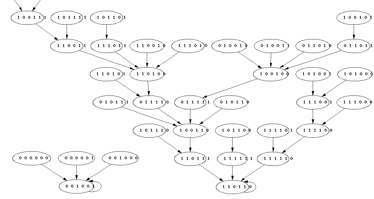
In the continuous system values for $x$ and $y$ could be negative, this is represented in the fixed point $(x,y)=(0,0)=(0,\_\_,0,\_,\_)$ of the discrete system.

In the next two sections we apply the above methods to two well-studied examples of gene regulatory networks, for which there exist delay differential equations models.

3 The Lac Operon

The lac operon is required for the transport and metabolism of lactose in Escherichia coli. It has been studied extensively, and Novick [12] showed in the 1950s that bistability is observed with artificial inducers. He observed that “preinduced” bacteria, that is bacteria grown in a high concentration of inducer, are able to maintain a high internal inducer concentration if subsequently grown in a low external inducer concentration. Novick, [12] calls this the “preinduction effect”. He observed, however, that if preinduced bacteria are transferred to a medium with no inducer, enzyme synthesis ceases immediately. The minimum concentration in which the high rate of synthesis of a preinduced culture can be maintained is called the maintenance concentration.

Novick’s experiments have led to various mathematical models of the lac operon whose steady state solutions show bistability, for example Yildirim [17], Wong[16], Boer [5].

We first give a brief overview of the functionality of the lac operon depicted in Fig. 4. In the absence of glucose for cellular metabolism, extracellular lactose is transported into the cell, either actively by permease or passively through diffusion. Inside the cell, $\beta$-galactosidase breaks up lactose into glucose, galactose, and allolactose. Allolactose binds to the repressor, which is usually bound to the operator region where it inhibits the transcription process, therefore the transcription process can proceed. RNA polymerase initiates transcription of the structural genes to produce mRNA, which is then translated into proteins, permease, and $\beta$-galactosidase.

Figure 4: Schematic representation of the lactose operon regulatory system from dnainfo.wikispaces.com

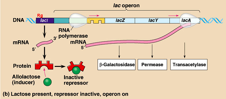
The system contains a positive feedback loop, with an increase in the concentration of allolactose, mRNA concentration increases, and therefore more $\beta$-galactosidase and permease are produced, which in turn leads to more internal lactose and allolactose. Positive (or negative) feedback loops are very common in biological systems because they allow for a rapid increase in concentration. In the case of the lac operon, the enzyme induction is an “all-or-none phenomenon”, with the first permease molecule extracellular lactose is transported into the cell, increasing the inducer concentration, and therefore increasing the probability of the appearance of another permease molecule, [12].

3.1 Boolean Model of Lac Operon

We derive a Boolean network for the gene regulatory network from the continuous model developed in [17] consisting of 5 equations. All its parameters were estimated from the biological literature and the equations were numerically solved for their steady states. The delay differential equations model predicts a bistable region for a medium external inducer concentration, which is in accordance to what has been observed experimentally by [12] and [3]. As in the continuous model, we take the following 5 variables for the Boolean model into account: messenger RNA $M$, $\beta$-galactosidase $B$, allolactose $A$, permease $P$, and internal lactose $L$.

We will show how to derive the Boolean equation for messenger RNA, the process for the other variables is similar and can be found in the appendix. In [17], the rate of change of mRNA is given by the following equation:

$$\frac{d}{dt}M(t)= \alpha_{M}\frac{1+K_{1}(e^{-\mu\tau_{M}}A_{\tau_{M}})^{n}}{K+K_{1}(e^{-\mu\tau_{M}}A_{\tau_{M}})^{n}}+\Gamma_{0}-\tilde{\gamma}_{M}M$$

$$= \alpha_{M}\frac{1+K_{1}(e^{-\mu\tau_{M}}A(t-\tau_{M}))^{n}}{K+K_{1}(e^{-\mu\tau_{M}}A(t-\tau_{M}))^{n}}+\Gamma_{0}-(\gamma_{M}+\mu)M,$$

where $n$ is the number of molecules of allolactose required to inactivate the repressor. $\frac{d}{dt}M(t)$ depends on $A$ at time $(t-\tau_{M})$ and $-(\gamma_{M}+\mu)M$ models the loss caused by dilution and degradation.

Under the presence of allolactose $A$, $\frac{d}{dt}M$ is non-negative, so the Boolean equation for mRNA is

$$f_{M}=x_{A_{\tau}},$$

where $A_{\tau}$ describes the allolactose concentration $A$ time $\tau_{M}$ ago.

If mRNA is present and no new mRNA is produced in the next time step, the concentration will decrease according to the degradation rate. To capture this in the Boolean model, we introduce the artificial variable $M_{\text{old}}$ as described in section 2.0.1. $M_{\text{old}}$ is “on”, if allolactose is absent, because then no new mRNA was produced. If no mRNA was produced for 2 time steps, its concentration is too low and we consider $M$ to be “off”. This results in the following equations:

$$f_{M} =x_{A_{\tau}}\vee(x_{M}\wedge\neg x_{M_{\text{old}}})$$

$$f_{M_{\text{old}}} =\neg x_{A_{\tau}}.$$

mRNA depends on $A$ time $\tau$ ago, so a new variable $A1$ is introduced, as described in 2.0.2 and we set

$$f_{M} =x_{A1}\vee(x_{M}\wedge\neg x_{M_{\text{old}}})$$

$$f_{M_{\text{old}}} =\neg x_{A1}$$

$$f_{A} =\ldots$$

$$f_{A1} =x_{A}.$$

We discretize the external inducer concentration $L_{e}$ to be “on”, if it is above the minimal maintenance concentration. The high external inducer concentration $L_{e_{\text{high}}}$ is “on”, if the concentration is at least (*), as shown in Fig 5.

Figure 5: Discretization of External Inducer

Using the method described above, accounting for degradation and delays, we derive the following Boolean model:
$\displaystyle f_{M}=x_{A1}\vee(x_{M}\wedge\neg x_{M_{\text{old}}})$ $\displaystyle f_{M1}=x_{M}$ $\displaystyle f_{M2}=x_{M1}$ $\displaystyle f_{M3}=x_{M2}$ $\displaystyle f_{M_{\text{old}}}=\neg x_{A1}$ $\displaystyle f_{B}=x_{M2}\vee x_{B}$ $\displaystyle f_{A}=(x_{B}\wedge x_{L})\vee(x_{L}\wedge x_{L_{e_{\text{high}}}})$ $\displaystyle\qquad\vee(x_{A}\wedge\neg x_{A_{\text{old}}})$ $\displaystyle f_{A1}=x_{A}$ $\displaystyle f_{A_{\text{old}}}=\neg x_{B}\vee\neg x_{L}$ $\displaystyle f_{L}=(x_{P}\wedge x_{L_{e}})\vee x_{L_{e_{\text{high}}}}$ $\displaystyle\qquad\vee[x_{L}\wedge\neg(x_{L_{\text{old}}}\wedge(x_{P}\vee x_{B}))]$ $\displaystyle f_{L_{\text{old}}}=\neg x_{P}\vee\neg x_{L_{e}}$ $\displaystyle f_{P}=x_{M3}\vee(x_{P}\wedge\neg x_{P_{\text{old}}})$ $\displaystyle f_{P_{\text{old}}}=\neg x_{M3}$ $\displaystyle f_{L_{e}}=x_{L_{e}}\vee x_{L_{e_{\text{high}}}}$ $\displaystyle f_{L_{e_{\text{high}}}}=x_{L_{e_{\text{high}}}}.$
We use the DVD simulation software, see section 1.1, to calculate that the system has 8 fixed points and no limit cycles.

As expected, a low external inducer concentration (last two variables are set to 0) drives the system to fixed points corresponding to the operon in the “off” state, points $1-3$ in table 1. If the concentration of the artificial external inducer is medium, but not high, the system results in the fixed points $4-7$ in table 1. With high external inducer concentration, the system settles in the remaining fixed point which corresponds to an induced operon.

	$M$	$M_{1}$	$M_{2}$	$M_{3}$	$M_{\text{old}}$	$B$	$A$	$A_{1}$	$A_{\text{old}}$	$L$	$L_{\text{old}}$	$P$	$P_{\text{old}}$	$L_{e}$	$L_{e_{\text{high}}}$
1	0	0	0	0	1	0	0	0	1	0	1	0	1	0	0
2	0	0	0	0	1	0	0	0	1	1	1	0	1	0	0
3	0	0	0	0	1	1	0	0	1	0	1	0	1	0	0
4	0	0	0	0	1	0	0	0	1	1	1	0	1	1	0
5	0	0	0	0	1	1	0	0	1	0	1	0	1	1	0
6	0	0	0	0	1	0	0	0	1	0	1	0	1	1	0
7	1	1	1	1	0	1	1	1	0	1	1	1	0	1	0
8	1	1	1	1	0	1	1	1	0	1	1	1	0	1	1

Table 1: Fixed Points of Lac Operon

For a medium inducer concentration, fixed point $4$ and $5$ are biologically not meaningful, because they correspond to states in which only the internal lactose or $\beta$-galactosidase concentration is present but no other substance. Fixed point $6$ corresponds to the “off” operon, fixed point $7$ to the “on” operon.

To show bistability, we analyze the behavior of the fixed points as we change the concentration rates of the external inducer. If we start in a state corresponding to fixed point $1$ and increase the inducer concentration to a medium concentration, the system settles down in fixed point $6$, corresponding to the “off” operon. If we start with state $8$, the system settles down in fixed point $7$, corresponding to the “on” operon. This is exactly what we expect from the solution of the delay differential equation: under a medium concentration of external inducer, the steady state depends on whether the cell was preinduced or not.

4 Lambda Phage

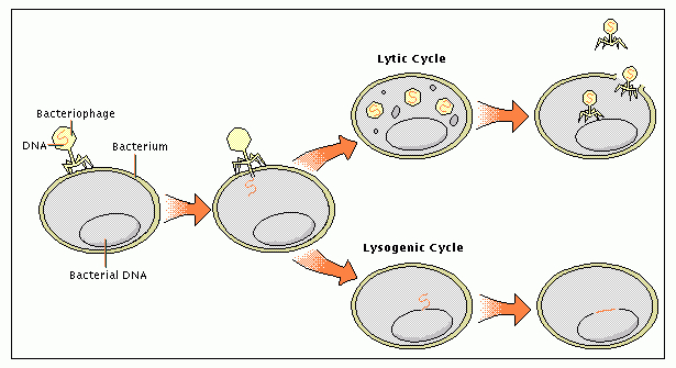
The virus lambda phage (phage $\lambda$) is a bacteriophage that infects Escherichia coli. After injecting its DNA into the host, the phage can enter the lytic pathway where it alters the host DNA to produce phage particles and then lyses the host cell, or it can enter the lysogenic pathway, where it is duplicated with every cell division and harmless until the cell is under stress, then it enters its lytic pathway. A schematic representation of the phage $\lambda$ switch is shown in Fig. 6. Interestingly, the lysogenic state is more stable than the genome itself [2]. A comprehensive explanation of the lambda phage switch can be found in [13].

Figure 6: The Life Cycle of Lambda Phages from www.mining.ubc.ca

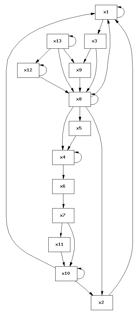
In [14] a delay differential equations model for the switch between lysogenic and lytic state of phage lambda is presented. This continuous model consists of four equations for the rate of change of the concentrations of cI and cro messenger RNA molecules, $cI$ and Cro monomers and of two equations for the dimer concentrations of $[CI_{2}]$ and $[Cro_{2}]$.

Bistable behavior depends on the degradation rate of $cI$, $\gamma_{cI}$. Numerical calculations show that the range for $\gamma_{cI}$ in which the systems has two fixed points, one corresponding to lysogeny, the other to lysis, is $0.0\text{min}^{-1}<\gamma_{cI}<0.35\text{min}^{-1}$. If the degradation rate of $cI$ is zero, the phage enters the lysogenic pathway, if it is above $0.35\text{min}^{-1}$, the lytic pathway. For a medium degradation rate of $cI$, phage lambda can enter the lytic or lysogenic pathway, so one needs to distinguish between three different degradation rates of $\gamma_{\text{cI}}$. Note that for the lambda phage a degradation rate drives the system in the bistable region, whereas for the lac operon an external inducer has that role. To distinguish between three states of $\gamma_{\text{cI}}$ in the Boolean model, the variable $\gamma_{\text{cI}_{high}}$ is introduced. To avoid wrong input, e.g., $\gamma_{\text{cI}}=0$ and $\gamma_{\text{cI}_{high}}=1$, $\gamma_{\text{cI}}$ is turned on, whenever $\gamma_{\text{cI}_{high}}=1$.

The delay caused by transcription is only 0.005 $\text{min}^{-1}$, whereas the delays caused by the translation of the monomers $cI$ and Cro are 0.06 and 0.24 $\text{min}^{-1}$. Therefore delay caused by transcription is neglected in the model.

For a high degradation rate, no $cI$ monomers are left after 1 timestep. We assume, that a small concentration of monomers is generated also if the Boolean expression that generates $cI$ is zero. As a consequence, if the degradation rate for $cI$ is zero, we assume that sufficient $cI$ monomers are produced to set $x_{CI}=1$ after one time step.

This results in the following Boolean model.

$$f_{M_{\text{cI}}} =x_{CI_{T}}\vee\overline{x_{Cro_{T}}}\vee(x_{M_{\text{cI}}}\wedge\overline{x_{M_{\text{cI}_{\text{old}}}}})$$

$$f_{M_{\text{cI}_{\text{old}}}} =\overline{x_{CI_{T}}}\wedge x_{Cro_{T}}$$

$$x_{M_{\text{cI}_{1}}} =x_{M_{\text{cI}}}$$

$$f_{M_{\text{cro}}} =\overline{x_{CI_{T}}}\vee(x_{M_{\text{cro}}}\wedge\overline{x_{{M_{\text{cro}}}_{\text{old}}}})$$

$$f_{{M_{\text{cro}}}_{\text{old}}} =x_{CI_{T}}$$

$$x_{M_{\text{cro}_{1}}} =x_{M_{\text{cro}}}$$

$$x_{M_{\text{cro}_{2}}} =x_{M_{\text{cro}_{1}}}$$

$$f_{CI_{T}} =\overline{\gamma_{\text{cI}_{1}}}\vee(\overline{\gamma_{\text{cI}_{\text{high}}}}\wedge(x_{M_{\text{cI}_{1}}}\vee(x_{CI_{T}}\wedge(\overline{x_{{CI_{T}}_{\text{old}}}}\vee\overline{\gamma_{\text{cI}}}))))$$

$$f_{{CI_{T}}_{\text{old}}} =\overline{x_{M_{\text{cI}_{1}}}}\vee\gamma_{\text{cI}_{\text{high}}}$$

$$f_{Cro_{T}} =x_{M_{\text{cro}_{2}}}\vee(x_{Cro_{T}}\wedge\overline{x_{{Cro_{T}}_{\text{old}}}})$$

$$f_{{Cro_{T}}_{\text{old}}} =\overline{x_{M_{\text{cro}_{2}}}}$$

$$f_{\gamma_{\text{cI}}} =\gamma_{\text{cI}}\vee\gamma_{\text{cI}_{\text{high}}}$$

$$f_{\gamma_{\text{cI}_{1}}} =\gamma_{\text{cI}}$$

$$f_{\gamma_{\text{cI}_{\text{high}}}} =\gamma_{\text{cI}_{\text{high}}}.$$

DVD simulation software [10] is used to calculate the fixed points and generate the dynamics in the bistable region. If the degradation rate is $0.0\text{min}^{-1}$, in the model the last three variables are off, the system results in the fixed point $[10101001001000]$ which corresponds to $[M_{cI}CI]$, a high $cI$ and low Cro concentration which means that the system is in the lysogenic state. If the degradation rate is medium, in the model the third last variable is on and the last two variables are off, there are two fixed points, $[01010110110110]$ and $[10101001001110]$, corresponding to $[M_{cro}Cro]$ and $[M_{cI}CI]$, respectively, lysogenic and lytic pathway. With a high degradation rate, in the model only the last variable of the last three variables is on, the system settles in the fixed point $[01010110110111]$, representing $[M_{cro}Cro]$. This means that the system is in the lytic state. All four fixed points are in accordance with the results found numerically and the switching behavior observed experimentally.

To investigate the bistable region, we start the model with an initialization that represents the lysogenic state. Increasing the degradation rate to a medium level results in the fixed point $[10101001001110]$, which is still the lysogenic state. Starting the model from a lytic state and decreasing the rate results in the fixed point $[01010110110110]$, representing the lytic state. Decreasing the rate even further finally results in the fixed point corresponding to the lysogenic state.

5 Discussion

The results presented in this paper show that biochemical networks that exhibit bistability can be modeled successfully using a Boolean network model, incorporating delays for variables, as needed. This was done by showing that continuous delay-differential equations models can be approximated by Boolean networks. The method presented here is quite general and could be applied to other types of biological networks. The examples show that simple Boolean models are able to capture steady states and complicated dynamics like hysteresis.

Boolean network models have the drawback that they do not give rise to exact concentration rates of the steady states because their discretization is too coarse grained. Discrete models with more than just two states, so called multi state models, might be suitable to give enough quantitative information about concentration rates while they are intuitive enough and easy to use for a wide range of scientists.

Appendix A Lac Operon

A.1 Dilution and Degradation

Since the degradation rates $\gamma_{M}$, $\gamma_{P}$, and $\gamma_{A}$ are close to $0.5\text{min}^{-1}$, we assume that mRNA, permease, and allolactose are degraded after 2 times steps. $\gamma_{L}$ and $\gamma_{B}$ are very small and will be neglected in our model.

A.2 $\beta$-galactosidase

For the $\beta$-galactosidase enzyme the equation in the continuous model is

$$\frac{dB}{dt} =\alpha_{B}e^{-\mu\tau_{B}}M_{\tau_{B}}-\tilde{\gamma}_{B}B$$

$$=\alpha_{B}e^{-\mu\tau_{B}}M_{\tau_{B}}-(\gamma_{B}+\mu)B.$$

Messenger RNA is translated into $\beta$-galactosidase which takes time $\tau_{B}$, so $f_{B}$ depends on $M_{\tau}$, the mRNA concentration time $\tau_{B}$ ago.

Since the degradation rate $\gamma_{B}$ is low, the Boolean model neglects the decrease due to dilution and degradation and we model $\beta$-galactosidase with the single equation

$$f_{B} =x_{M_{\tau}}\vee x_{B}.$$

A.3 Allolactose $A$

$$\frac{dA}{dt} =\alpha_{A}B\frac{L}{K_{L}+L}-\beta_{A}B\frac{A}{K_{A}+A}-\tilde{\gamma}_{A}A$$

Allolactose is gained by conversion of lactose and reduced by the loss via conversion to glucose and galactose, both mediated by $\beta$-galactosidase. Like for mRNA, we use an extra variable $A_{\text{old}}$ to capture the loss of allolactose due to dilution and degradation.

$$f_{A} =(x_{B}\wedge x_{L})\vee(x_{A}\wedge\neg x_{A_{\text{old}}})$$ (1)

$$f_{A_{\text{old}}} =\neg(x_{B}\wedge x_{L})$$

$$=\neg x_{B}\vee\neg x_{L}$$

Notice that 1 does not depend on any delayed variables.

A.4 Internal Lactose $L$

For internal lactose, Yildirim’s model suggests the following equation

$$\frac{dL}{dt}= \alpha_{L}P\frac{L_{e}}{K_{L_{e}}+L_{e}}-\beta_{L}P\frac{L}{K_{L_{1}}+L}$$

$$-\beta_{L_{2}}B\frac{L}{K_{L_{2}}+L}-\tilde{\gamma}_{L}L.$$

The degradation term $\gamma_{L}$ is low enough to be ignored in the discrete model. Lactose is broken down into glucose, galactose and allolactose by $\beta$-galactosidase, and permease actively transports lactose in and out of the cell. Again, since permease and $\beta$-galactosidase reduce the internal lactose concentration, we introduce the extra variable $L_{\text{old}}$ to turn $L$ off, if it has not been produced and if permease or $\beta$-galactosidase are present to reduce it.

$$f_{L} =(x_{P}\wedge x_{L_{e}})\vee[x_{L}\wedge\neg(x_{L_{\text{old}}}\wedge(x_{P}\vee x_{B}))]$$

$$f_{L_{\text{old}}} =\neg(x_{P}\wedge x_{L_{e}})$$

$$=\neg x_{P}\vee\neg x_{L_{e}}$$

A.5 Permease $P$

$$\frac{dP}{dt} =\alpha_{P}e^{-\mu(\tau_{P}+\tau_{B})}M_{\tau_{P}+\tau_{B}}-\tilde{\gamma}_{p}P$$

Messenger RNA is translated into permease, so the permease concentration $P$ is directly proportional to the mRNA concentration $M$ at time $(\tau_{P}+\tau_{B})$ ago and dilution and degradation reduce permease concentration, which is why $P_{\text{old}}$ is used in the Boolean model.

$$f_{P} =x_{M_{\tau}}\vee(x_{P}\wedge\neg x_{P_{\text{old}}})$$

$$f_{P_{\text{old}}} =\neg x_{M_{\tau}}.$$

Appendix B Lambda Phage

Renumerating the equations results in

$$f_{1} =x_{8}\vee\overline{x_{10}}\vee(x_{1}\wedge\overline{x_{2}})$$

$$f_{2} =\overline{x_{8}}\wedge x_{10}$$

$$f_{3} =x_{1}$$

$$f_{4} =\overline{x_{8}}\vee(x_{4}\wedge\overline{x_{5}})$$

$$f_{5} =x_{8}$$

$$f_{6} =x_{4}$$

$$f_{7} =x_{6}$$

$$f_{8} =\overline{x_{13}}\vee(\overline{x_{14}}\wedge(x_{3}\vee(x_{8}\wedge(\overline{x_{9}}\vee\overline{x_{12}}))))$$

$$f_{9} =\overline{x_{3}}\vee x_{14}$$

$$f_{10} =x_{7}\vee(x_{10}\wedge\overline{x_{11}})$$

$$f_{11} =\overline{x_{7}}$$

$$f_{12} =x_{12}\vee x_{14}$$

$$f_{13} =x_{12}$$

$$f_{14} =x_{14}.$$

The Boolean model has the dependency graph shown in Fig. 7.

Figure 7: Dependency graph of the Boolean model for Lambda Phage

References

- [1] R. Albert and H. Othmer, The topology of the regulatory interactions predicts the expression pattern of the segment polarity genes in drosophila melanogaster, 2003.
- [2] E. Aurell and K. Sneppen, Epigenetics as a first exit problem, Phys. Rev. Lett. 88 (2002), no. 4, 048101.
- [3] Melvin Cohn and Kengo Horibata, Inhibition by glucose of the induced synthesis of the -galactoside-enzyme system of escherichia coli. analysis of maintenance, J Bacteriol. 78 (1959), 601–612.
- [4] Carsten Conradi, Jörg Stelling, and Jörg Raisch, Structure discrimination of continuous models for biochemical reaction networks via finite state machines, Proc. IEEE Int. Symposium on Intelligent Control (Mexico City, Mexico), 2001, p. 138?143.
- [5] Rob de Boer, Theoretical biology, p. 9.
- [6] R. Edwards, H. T. Siegelmann, K. Aziza, and L. Glass, Symbolic dynamics and computation in model gene networks, Chaos 11 (2001), 160–169.
- [7] Nir Friedman, Michal Linial, and Iftach Nachman, Using bayesian networks to analyze expression data, Journal of Computational Biology 7 (2000), 601–620.
- [8] F. Jacob and J. Monod, Genetic regulatory mechanisms in the synthesis of proteins., J Mol Biol 3 (1961), 318–356.
- [9] S. A. Kauffman, Metabolic stability and epigenesis in randomly constructed genetic nets, Journal of Theoretical Biology 22 (1969), no. 3, 437–467.
- [10] Reinhard Laubenbacher and Abdul Jarrah, Dvd - discrete visualizer of dynamics.
- [11] Luis Mendoza and Ioannis Xenarios, A method for the generation of standardized qualitative dynamical systems of regulatory networks, Theoretical Biology and Medical Modelling 3 (2006), no. 1, 13+.
- [12] A. Novick and M. Weiner, Enzyme induction as an all-or-none phenomenon., Proc Natl Acad Sci U S A 43 (1957), no. 7, 553–66.
- [13] Mark Ptashne, A genetic switch phage lambda revisited, 3rd ed., Cold Spring Harbor Laboritory Press, 2004.
- [14] Moisés Santillán and Michael C. Mackey, Why the lysogenic state of phage lambda is so stable: a mathematical modeling approach., Biophys J 86 (2004), 75–84.
- [15] T. Tian and K. Burrage, Stochastic models for regulatory networks of the genetic toggle switch., Proc Natl Acad Sci U S A 103 (2006), no. 22, 8372–8377.
- [16] P. Wong, S. Gladney, and J. D. Keasling, Mathematical model of the lac operon: inducer exclusion, catabolite repression, and diauxic growth on glucose and lactose., Biotechnology progress 13 (1997), no. 2, 132–143.
- [17] N. Yildirim and M. C. Mackey, Feedback regulation in the lactose operon: a mathematical modeling study and comparison with experimental data., Biophys J 84 (2003), no. 5, 2841–2851.