Early exercise boundary for American type of floating strike Asian option and its numerical approximation

Tomáš Bokes and Daniel Ševčovič
Department of Applied Mathematics and Statistics,
Faculty of Mathematics, Physics and Informatics,
Comenius University, 842 48 Bratislava, Slovak Republic
Abstract

In this paper we generalize and analyze the model for pricing American-style Asian options due to (?) by including a continuous dividend rate q𝑞q and a general method of averaging of the floating strike. We focus on the qualitative and quantitative analysis of the early exercise boundary. The first order Taylor series expansion of the early exercise boundary close to expiry is constructed. We furthermore propose an efficient numerical algorithm for determining the early exercise boundary position based on the front fixing method. Construction of the algorithm is based on a solution to a nonlocal parabolic partial differential equation for the transformed variable representing the synthesized portfolio. Various numerical results and comparisons of our numerical method and the method developed by (?) are presented.

Keywords: option pricing, American-style of Asian options, early exercise boundary, limiting behavior close to expiry

AMS-MOS classification: 35K15, 35K55, 90A09, 91B28

1 Introduction

Evolution of trading systems influences the development of financial derivatives market. First, simple derivatives like forwards and plain vanilla options were used to hedge the risk of a portfolio. Progress in pricing these simple financial instruments pushed traders into inventing less predictable and more complex derivatives. Using financial derivatives with more complicated pay-offs brings into attention also new mathematical problems. Asian options belong to a group of the so-called path-dependent options. Their pay-off diagrams depend on the spot value of the underlying during the whole or some part(s) of the life span of the option. Usually Asian options depend on the (arithmetic or geometric) average of the spot price of the underlying. They can be also used as a useful tool for hedging highly volatile assets or goods. Since the price of an underlying varies during the life span of the option the holder of the Asian option can be secured for the risk a sudden price jumping to an undesirable region (too high for the call option holder or too low for the put option holder). Among path dependent options Asian options plays an important role as they are quite common in currency and commodity markets like e.g. oil industry (cf. (???????????)).

In this paper we focus on the so-called floating strike Asian call or put options whose strike price depends on the averaged path history of the underlying asset. More precisely, we are interested in pricing American-style Asian call and put options having the pay-off functions VT(S,A)=(SA)+subscript𝑉𝑇𝑆𝐴superscript𝑆𝐴V_{T}(S,A)=(S-A)^{+} and VT(S,A)=(AS)+subscript𝑉𝑇𝑆𝐴superscript𝐴𝑆V_{T}(S,A)=(A-S)^{+}, resp. The strike price A𝐴A is given as an average of the underlying over the time history [0,T]0𝑇[0,T]. We are analyzing the early exercise boundary for American-style Asian option (cf. (???)). Recall that American-style options can be exercised at any time until the maturity T𝑇T. The holder of such an option has the right to exercise it or to keep it depending on the spot price of the underlying Stsubscript𝑆𝑡S_{t} at time t𝑡t and its history {Su,0ut}subscript𝑆𝑢0𝑢𝑡\{S_{u},0\leq u\leq t\} prior the time t𝑡t. The boundary between ”continuation” and ”stopping” regions plays an important role in pricing American-style of options. It can be described by the mapping St:tSt:subscriptsuperscript𝑆𝑡maps-to𝑡subscriptsuperscript𝑆𝑡S^{*}_{t}:t\mapsto S^{*}_{t}, where Stsubscriptsuperscript𝑆𝑡S^{*}_{t} is the so-called early exercise boundary (cf. (?????????).

The paper is organized as follows. In the next section, we discuss the probabilistic model for valuation of American type Asian options with a floating strike given in the form of an average of the underlying asset price. The model is based on conditioned expected values and theory of martingales. In the third section, we present a general result enabling us to calculate the value of the limit of the early exercise boundary at expiry. We also calculate the analytical integral formula for an option with continuous geometric average and an approximation for the value of an option with a continuous arithmetic average. The main result of this section is the approximation formula for the first order Taylor series approximation of the early exercise boundary near to expiry. Similarly as in the case of plain vanilla call options, we show that the leading order of the expansion is the square root Tt𝑇𝑡\sqrt{T-t} of the time Tt𝑇𝑡T-t remaining to maturity. In the fourth section, we present the fixed domain transformation method yielding a nonlocal nonlinear parabolic partial differential equation for pricing the synthesized portfolio for an Asian option. We also present an efficient and robust numerical scheme for construction of an approximation of the solution to the governing system consisting of a partial differential equation with an algebraic constraint. In the last part of this section we present also the results of the presented method on some examples.

2 A probabilistic approach for pricing of American-Style of Asian options

The main purpose of this section is to derive an integral equation for valuation of the early exercise boundary of an American-style Asian option paying continuous dividends. We follow the ideas of derivation due to (?). Their formula for a floating strike option was derived using the theory of martingales and conditioned expected values. We extend their formula to Asian options on underlying paying non-zero dividend yield and having a general form of floating strike averaging. In a more detail, we discuss geometric, arithmetic and weighted arithmetic averaging operator.

The pricing model is based on the assumption on the stochastic behavior of the underlying asset in time. Throughout the paper we shall assume that the underlying asset price Stsubscript𝑆𝑡S_{t} is driven by a stochastic process satisfying the following stochastic differential equation

dSt=(rq)Stdt+σStdWtP,0tT.formulae-sequence𝑑subscript𝑆𝑡𝑟𝑞subscript𝑆𝑡𝑑𝑡𝜎subscript𝑆𝑡𝑑superscriptsubscript𝑊𝑡𝑃0𝑡𝑇dS_{t}=(r-q)S_{t}\ dt+\sigma S_{t}\ dW_{t}^{P},\quad 0\leq t\leq T. (1)

It starts almost surely from the initial price S0>0subscript𝑆00S_{0}>0. Here the constant parameter r>0𝑟0r>0 denotes the risk-free interest rate whereas q0𝑞0q\geq 0 is a continuous dividend rate. The constant parameter σ𝜎\sigma stands for the volatility of the underlying asset returns and WtPsuperscriptsubscript𝑊𝑡𝑃W_{t}^{P} is a standard Brownian motion with respect to the standard risk-neutral probability measure P𝑃P. A solution to equation (1) corresponds to the geometric Brownian motion

St=S0e(rq12σ2)t+σWtP,0tT.formulae-sequencesubscript𝑆𝑡subscript𝑆0superscript𝑒𝑟𝑞12superscript𝜎2𝑡𝜎superscriptsubscript𝑊𝑡𝑃0𝑡𝑇S_{t}=S_{0}e^{(r-q-\frac{1}{2}\sigma^{2})t+\sigma W_{t}^{P}},\quad 0\leq t\leq T.

We shall derive an integral equation determining the value of an American-style Asian option with a floating strike. If we define the optimal stopping time as Tsuperscript𝑇T^{*}, the pay-off of the option is set by

VT=(ρ(STAT))+,subscript𝑉superscript𝑇superscript𝜌subscript𝑆superscript𝑇subscript𝐴superscript𝑇V_{T^{*}}=\Big{(}\rho(S_{T^{*}}-A_{T^{*}})\Big{)}^{+},

where Vtsubscript𝑉𝑡V_{t} is the value of the option at time t𝑡t, Atsubscript𝐴𝑡A_{t} is a continuous average of the underlying asset value during the interval [0,t]0𝑡[0,t] and ρ=1𝜌1\rho=1 for a call option and ρ=1𝜌1\rho=-1 for a put option. We may consider several different types of continuous averages presented in Table 1.

Table 1: Classification of averaging methods.
arithmetic average geometric average weighted arithmetic average
At=1t0tSu𝑑usubscript𝐴𝑡1𝑡superscriptsubscript0𝑡subscript𝑆𝑢differential-d𝑢A_{t}=\frac{1}{t}\int_{0}^{t}{S_{u}}\,du lnAt=1t0tlnSudusubscript𝐴𝑡1𝑡superscriptsubscript0𝑡subscript𝑆𝑢𝑑𝑢\ln{A_{t}}=\frac{1}{t}\int_{0}^{t}{\ln{S_{u}}}\,du At=10ta(s)𝑑s0ta(tu)Su𝑑usubscript𝐴𝑡1superscriptsubscript0𝑡𝑎𝑠differential-d𝑠superscriptsubscript0𝑡𝑎𝑡𝑢subscript𝑆𝑢differential-d𝑢A_{t}=\frac{1}{\int_{0}^{t}{a(s)}\ ds}\int_{0}^{t}{a(t-u)S_{u}}\,du

In the case of a weighted arithmetically averaged floating strike Asian option the kernel function a(.)0a(.)\geq 0 with the property 0a(s)𝑑s<superscriptsubscript0𝑎𝑠differential-d𝑠\int_{0}^{\infty}{a(s)}\ ds<\infty is usually defined as a(s)=eλs𝑎𝑠superscript𝑒𝜆𝑠a(s)=e^{-\lambda s} where λ>0𝜆0\lambda>0 is constant.

According to (?), the American-style contingent claims can be priced by the conditioned expectations approach. The option price can be calculated by considering all possible stopping times in the interval [t,T]𝑡𝑇[t,T]

V(t,S,A)=esssups𝒯[t,T]𝔼tP[er(st)(ρ(SsAs))+|St=S,At=A],𝑉𝑡𝑆𝐴esssubscriptsupremum𝑠subscript𝒯𝑡𝑇superscriptsubscript𝔼𝑡𝑃delimited-[]formulae-sequenceconditionalsuperscript𝑒𝑟𝑠𝑡superscript𝜌subscript𝑆𝑠subscript𝐴𝑠subscript𝑆𝑡𝑆subscript𝐴𝑡𝐴V(t,S,A)=\hbox{ess}\!\!\!\!\sup_{s\in\mathcal{T}_{[t,T]}}\ \mathbb{E}_{t}^{P}\Big{[}e^{-r(s-t)}\Big{(}\rho(S_{s}-A_{s})\Big{)}^{+}\Big{|}S_{t}=S,A_{t}=A\Big{]},

where 𝒯[t,T]subscript𝒯𝑡𝑇\mathcal{T}_{[t,T]} denotes the set of all stopping times in the interval [t,T]𝑡𝑇[t,T] and 𝔼tP[X]=𝔼P[X|t]superscriptsubscript𝔼𝑡𝑃delimited-[]𝑋superscript𝔼𝑃delimited-[]conditional𝑋subscript𝑡{\mathbb{E}}_{t}^{P}[X]={\mathbb{E}}^{P}[X|\mathcal{F}_{t}] is the conditioned expectation with information available at time t𝑡t (the information set is represented by the filtration tsubscript𝑡\mathcal{F}_{t} of the σ𝜎\sigma-algebra \mathcal{F} where the Brownian motion is supported). To simplify the formula we change the probability measure by the martingale

ηt=e(rq)tStS0=e12σ2t+σWtPsubscript𝜂𝑡superscript𝑒𝑟𝑞𝑡subscript𝑆𝑡subscript𝑆0superscript𝑒12superscript𝜎2𝑡𝜎superscriptsubscript𝑊𝑡𝑃\eta_{t}=e^{-(r-q)t}\frac{S_{t}}{S_{0}}=e^{-\frac{1}{2}\sigma^{2}t+\sigma W_{t}^{P}}

the new probability measure 𝒬𝒬\mathcal{Q} being defined as d𝒬=ηTdP𝑑𝒬subscript𝜂𝑇𝑑𝑃d\mathcal{Q}=\eta_{T}\,dP. According to Girsanov’s theorem (?), the process

Wt𝒬=WtPσtsuperscriptsubscript𝑊𝑡𝒬superscriptsubscript𝑊𝑡𝑃𝜎𝑡W_{t}^{\mathcal{Q}}=W_{t}^{P}-\sigma t

is a standard Brownian motion with respect to the measure 𝒬𝒬\mathcal{Q}. The value of the underlying asset price under this measure is defined by

St=S0e(rq+12σ2)t+σWt𝒬.subscript𝑆𝑡subscript𝑆0superscript𝑒𝑟𝑞12superscript𝜎2𝑡𝜎superscriptsubscript𝑊𝑡𝒬S_{t}=S_{0}e^{(r-q+\frac{1}{2}\sigma^{2})t+\sigma W_{t}^{\mathcal{Q}}}. (2)

All assets priced under this measure are 𝒬𝒬\mathcal{Q}-martingales when discounted by the underlying price. According to this fact, we can reduce the dimension of stochastic variables. We introduce a new variable xt=AtStsubscript𝑥𝑡subscript𝐴𝑡subscript𝑆𝑡x_{t}=\frac{A_{t}}{S_{t}}. We obtain:

V(t,S,A)𝑉𝑡𝑆𝐴\displaystyle V(t,S,A) =\displaystyle= esssups𝒯[t,T]𝔼tP[er(st)(ρ(SsAs))+|St=S,At=A]esssubscriptsupremum𝑠subscript𝒯𝑡𝑇superscriptsubscript𝔼𝑡𝑃delimited-[]formulae-sequenceconditionalsuperscript𝑒𝑟𝑠𝑡superscript𝜌subscript𝑆𝑠subscript𝐴𝑠subscript𝑆𝑡𝑆subscript𝐴𝑡𝐴\displaystyle\hbox{ess}\!\!\!\!\sup_{\!\!\!\!\!\!s\in\mathcal{T}_{[t,T]}}\ \mathbb{E}_{t}^{P}\Big{[}e^{-r(s-t)}\Big{(}\rho(S_{s}-A_{s})\Big{)}^{+}\Big{|}S_{t}=S,A_{t}=A\Big{]}
=\displaystyle= esssups𝒯[t,T]𝔼t𝒬[ηtηTer(st)(ρ(SsAs))+|St=S,At=A]esssubscriptsupremum𝑠subscript𝒯𝑡𝑇superscriptsubscript𝔼𝑡𝒬delimited-[]formulae-sequenceconditionalsubscript𝜂𝑡subscript𝜂𝑇superscript𝑒𝑟𝑠𝑡superscript𝜌subscript𝑆𝑠subscript𝐴𝑠subscript𝑆𝑡𝑆subscript𝐴𝑡𝐴\displaystyle\hbox{ess}\!\!\!\!\sup_{s\in\mathcal{T}_{[t,T]}}\ \mathbb{E}_{t}^{\mathcal{Q}}\Big{[}\frac{\eta_{t}}{\eta_{T}}e^{-r(s-t)}\Big{(}\rho(S_{s}-A_{s})\Big{)}^{+}\Big{|}S_{t}=S,A_{t}=A\Big{]}
=\displaystyle= esssups𝒯[t,T]𝔼t𝒬[eq(st)St(ρ(1AsSs))+|St=S,At=A]esssubscriptsupremum𝑠subscript𝒯𝑡𝑇superscriptsubscript𝔼𝑡𝒬delimited-[]formulae-sequenceconditionalsuperscript𝑒𝑞𝑠𝑡subscript𝑆𝑡superscript𝜌1subscript𝐴𝑠subscript𝑆𝑠subscript𝑆𝑡𝑆subscript𝐴𝑡𝐴\displaystyle\hbox{ess}\!\!\!\!\sup_{s\in\mathcal{T}_{[t,T]}}\ \mathbb{E}_{t}^{\mathcal{Q}}\Big{[}e^{-q(s-t)}S_{t}\Big{(}\rho\Big{(}1-\frac{A_{s}}{S_{s}}\Big{)}\Big{)}^{+}\Big{|}S_{t}=S,A_{t}=A\Big{]}
=\displaystyle= esssups𝒯[t,T]eq(st)S𝔼t𝒬[(ρ(1xs))+|St=S,At=A].esssubscriptsupremum𝑠subscript𝒯𝑡𝑇superscript𝑒𝑞𝑠𝑡𝑆superscriptsubscript𝔼𝑡𝒬delimited-[]formulae-sequenceconditionalsuperscript𝜌1subscript𝑥𝑠subscript𝑆𝑡𝑆subscript𝐴𝑡𝐴\displaystyle\hbox{ess}\!\!\!\!\sup_{s\in\mathcal{T}_{[t,T]}}\ e^{-q(s-t)}S\ \mathbb{E}_{t}^{\mathcal{Q}}\Big{[}\Big{(}\rho(1-x_{s})\Big{)}^{+}\Big{|}S_{t}=S,A_{t}=A\Big{]}.

The last expression can be rewritten in terms of the new variable x=AS𝑥𝐴𝑆x=\frac{A}{S} as follows:

V~(t,x)=eqtV(t,S,A)S=eqTt𝔼t𝒬[(ρ(1xTt))+],~𝑉𝑡𝑥superscript𝑒𝑞𝑡𝑉𝑡𝑆𝐴𝑆superscript𝑒𝑞subscriptsuperscript𝑇𝑡superscriptsubscript𝔼𝑡𝒬delimited-[]superscript𝜌1subscript𝑥subscriptsuperscript𝑇𝑡\widetilde{V}(t,x)=e^{-qt}\frac{V(t,S,A)}{S}=e^{-qT^{*}_{t}}\ \mathbb{E}_{t}^{\mathcal{Q}}\Big{[}\Big{(}\rho(1-x_{T^{*}_{t}})\Big{)}^{+}\Big{]}, (3)

where Tt=inf{s[t,T]|xs=xs}subscriptsuperscript𝑇𝑡infimumconditional-set𝑠𝑡𝑇subscript𝑥𝑠superscriptsubscript𝑥𝑠T^{*}_{t}=\inf\{s\in[t,T]|x_{s}=x_{s}^{*}\} and the function [0,T]txtcontains0𝑇𝑡maps-tosubscriptsuperscript𝑥𝑡[0,T]\ni t\mapsto x^{*}_{t}\in\mathbb{R} describes the early exercise boundary.

Definition 2.1

The stopping region 𝒮𝒮\mathcal{S} and continuation region 𝒞𝒞\mathcal{C} for American-style Asian call and put options (3) are defined by

𝒮call=𝒞put={(t,x)|t[0,T],0x<xt},𝒞call=𝒮put={(t,x)|t[0,T],xt<x<}.formulae-sequencesubscript𝒮𝑐𝑎𝑙𝑙subscript𝒞𝑝𝑢𝑡conditional-set𝑡𝑥formulae-sequence𝑡0𝑇0𝑥subscriptsuperscript𝑥𝑡subscript𝒞𝑐𝑎𝑙𝑙subscript𝒮𝑝𝑢𝑡conditional-set𝑡𝑥formulae-sequence𝑡0𝑇subscriptsuperscript𝑥𝑡𝑥\displaystyle\mathcal{S}_{call}=\mathcal{C}_{put}=\{(t,x)|t\in[0,T],0\leq x<x^{*}_{t}\},\ \mathcal{C}_{call}=\mathcal{S}_{put}=\{(t,x)|t\in[0,T],x^{*}_{t}<x<\infty\}.

where [0,T]txt0𝑇𝑡maps-tosubscriptsuperscript𝑥𝑡[0,T]\in t\mapsto x^{*}_{t}\in\mathbb{R} is a continuous function determining the early exercise boundary. By 𝟏𝒮()subscript1𝒮{\bf 1}_{\mathcal{S}}(\cdot) we shall denote the indicator function of the set 𝒮𝒮\mathcal{S}, i.e. 𝟏𝒮(t,y)=1subscript1𝒮𝑡𝑦1{\bf 1}_{\mathcal{S}}(t,y)=1 for (t,y)𝒮𝑡𝑦𝒮(t,y)\in\mathcal{S} and 𝟏𝒮(t,y)=0subscript1𝒮𝑡𝑦0{\bf 1}_{\mathcal{S}}(t,y)=0 otherwise.

In the following theorem we present a solution to the pricing problem with one stochastic variable xtsubscript𝑥𝑡x_{t} formulated in (3). It is a generalization of the result by (?) and (?) for the case of a nontrivial dividend rate q0𝑞0q\geq 0 and a general form of the averaging of the floating strike price.

Theorem 2.1

The value V~(t,xt)~𝑉𝑡subscript𝑥𝑡\widetilde{V}(t,x_{t}) of the American-style floating strike Asian call (ρ=1𝜌1\rho=1) or put option (ρ=1𝜌1\rho=-1) on the underlying asset xtsubscript𝑥𝑡x_{t} paying continuous dividends with a rate q0𝑞0q\geq 0 is given by V~(t,xt)=v~(t,xt)+e~(t,xt)~𝑉𝑡subscript𝑥𝑡~𝑣𝑡subscript𝑥𝑡~𝑒𝑡subscript𝑥𝑡\widetilde{V}(t,x_{t})=\widetilde{v}(t,x_{t})+\widetilde{e}(t,x_{t}), where

v~(t,xt)𝔼t𝒬[eqT(ρ(1xT))+],~𝑣𝑡subscript𝑥𝑡superscriptsubscript𝔼𝑡𝒬delimited-[]superscript𝑒𝑞𝑇superscript𝜌1subscript𝑥𝑇\displaystyle\widetilde{v}(t,x_{t})\equiv\mathbb{E}_{t}^{\mathcal{Q}}\Big{[}e^{-qT}\Big{(}\rho(1-x_{T})\Big{)}^{+}\Big{]}, (4)
e~(t,xt)𝔼t𝒬[tTρequxu𝟏𝒮(u,xu)(dAuAu(rqxu1)du)],~𝑒𝑡subscript𝑥𝑡superscriptsubscript𝔼𝑡𝒬delimited-[]superscriptsubscript𝑡𝑇𝜌superscript𝑒𝑞𝑢subscript𝑥𝑢subscript1𝒮𝑢subscript𝑥𝑢𝑑subscript𝐴𝑢subscript𝐴𝑢𝑟𝑞superscriptsubscript𝑥𝑢1𝑑𝑢\displaystyle\widetilde{e}(t,x_{t})\equiv\mathbb{E}_{t}^{\mathcal{Q}}\Big{[}\int_{t}^{T}{\rho e^{-qu}x_{u}{\bf 1}_{\mathcal{S}}(u,x_{u})\Big{(}\frac{dA_{u}}{A_{u}}-(r-qx_{u}^{-1})du\Big{)}}\Big{]}, (5)

with the average given by the function Atsubscript𝐴𝑡A_{t} and stopping region 𝒮𝒮\mathcal{S}.

In the proof of Theorem 2.1 we shall use the next lemma.

Lemma 2.1

The auxiliary variable xt=AtStsubscript𝑥𝑡subscript𝐴𝑡subscript𝑆𝑡x_{t}=\frac{A_{t}}{S_{t}} satisfies the following stochastic differential equation:

dxt=xtdAtAt(rq)xtdtσxtdWt𝒬.𝑑subscript𝑥𝑡subscript𝑥𝑡𝑑subscript𝐴𝑡subscript𝐴𝑡𝑟𝑞subscript𝑥𝑡𝑑𝑡𝜎subscript𝑥𝑡𝑑superscriptsubscript𝑊𝑡𝒬dx_{t}=x_{t}\frac{dA_{t}}{A_{t}}-(r-q)x_{t}\ dt-\sigma x_{t}\ dW_{t}^{\mathcal{Q}}.

P r o o f: [of Lemma 2.1] We express the differential dxt=d(AtSt)𝑑subscript𝑥𝑡𝑑subscript𝐴𝑡subscript𝑆𝑡dx_{t}=d\Big{(}\frac{A_{t}}{S_{t}}\Big{)} as

dxt=1StdAtAtSt2dSt+AtSt3(dSt)2=xtdAtAt(rq)xtdtσxtdWt𝒬,𝑑subscript𝑥𝑡1subscript𝑆𝑡𝑑subscript𝐴𝑡subscript𝐴𝑡superscriptsubscript𝑆𝑡2𝑑subscript𝑆𝑡subscript𝐴𝑡superscriptsubscript𝑆𝑡3superscript𝑑subscript𝑆𝑡2subscript𝑥𝑡𝑑subscript𝐴𝑡subscript𝐴𝑡𝑟𝑞subscript𝑥𝑡𝑑𝑡𝜎subscript𝑥𝑡𝑑superscriptsubscript𝑊𝑡𝒬dx_{t}=\frac{1}{S_{t}}dA_{t}-\frac{A_{t}}{S_{t}^{2}}dS_{t}+\frac{A_{t}}{S_{t}^{3}}(dS_{t})^{2}=x_{t}\frac{dA_{t}}{A_{t}}-(r-q)x_{t}\ dt-\sigma x_{t}\ dW_{t}^{\mathcal{Q}},

and the proof of lemma follows. \square

Notice that, when comparing to the original expression due to (?) with a zero dividend rate q=0𝑞0q=0 the only difference is that the parameter r𝑟r is replaced by the term rq𝑟𝑞r-q.

The value of dAtAt𝑑subscript𝐴𝑡subscript𝐴𝑡\frac{dA_{t}}{A_{t}} depends on the method of averaging of the underlying asset used in valuation. The expressions for continuous averages are presented in Table 2. In this table we present the value of the weighted arithmetic average restricted to the kernel a(s)=eλs𝑎𝑠superscript𝑒𝜆𝑠a(s)=e^{-\lambda s}.

Table 2: The value of the differential dAtAt𝑑subscript𝐴𝑡subscript𝐴𝑡\frac{dA_{t}}{A_{t}}.
arithmetic average geometric average weighted arithmetic average
dAtaAta=1t(1xta1)dt𝑑subscriptsuperscript𝐴𝑎𝑡subscriptsuperscript𝐴𝑎𝑡1𝑡1subscriptsuperscript𝑥𝑎𝑡1𝑑𝑡\frac{dA^{a}_{t}}{A^{a}_{t}}=\frac{1}{t}\Big{(}\frac{1}{x^{a}_{t}}-1\Big{)}\ dt dAtgAtg=1tlnxtgdt𝑑subscriptsuperscript𝐴𝑔𝑡subscriptsuperscript𝐴𝑔𝑡1𝑡subscriptsuperscript𝑥𝑔𝑡𝑑𝑡\frac{dA^{g}_{t}}{A^{g}_{t}}=-\frac{1}{t}\ln{x^{g}_{t}}\ dt dAtwaAtwa=λ1eλt(1xtwa1)dt𝑑subscriptsuperscript𝐴𝑤𝑎𝑡subscriptsuperscript𝐴𝑤𝑎𝑡𝜆1superscript𝑒𝜆𝑡1subscriptsuperscript𝑥𝑤𝑎𝑡1𝑑𝑡\frac{dA^{wa}_{t}}{A^{wa}_{t}}=\frac{\lambda}{1-e^{-\lambda t}}\Big{(}\frac{1}{x^{wa}_{t}}-1\Big{)}\ dt

P r o o f: [of Theorem 2.1] We follow the proof of the original result by (?) and we include necessary modifications related to the form of averaging and the fact that q0𝑞0q\geq 0.

First, we suppose that (t,x)𝒞𝑡𝑥𝒞(t,x)\in\mathcal{C}. The option is held and so we can apply Itō’s lemma to calculate the differential

dV~𝑑~𝑉\displaystyle d\widetilde{V} =\displaystyle= V~xdx+122V~x2(dx)2+V~tdt~𝑉𝑥𝑑𝑥12superscript2~𝑉superscript𝑥2superscript𝑑𝑥2~𝑉𝑡𝑑𝑡\displaystyle\frac{\partial\widetilde{V}}{\partial x}dx+\frac{1}{2}\frac{\partial^{2}\widetilde{V}}{\partial x^{2}}(dx)^{2}+\frac{\partial\widetilde{V}}{\partial t}dt
=\displaystyle= xV~xdAA+[(rq)xV~x+12σ2x22V~x2+V~t]dtσxV~xdW𝒬𝑥~𝑉𝑥𝑑𝐴𝐴delimited-[]𝑟𝑞𝑥~𝑉𝑥12superscript𝜎2superscript𝑥2superscript2~𝑉superscript𝑥2~𝑉𝑡𝑑𝑡𝜎𝑥~𝑉𝑥𝑑superscript𝑊𝒬\displaystyle x\frac{\partial\widetilde{V}}{\partial x}\frac{dA}{A}+\Big{[}-(r-q)x\frac{\partial\widetilde{V}}{\partial x}+\frac{1}{2}\sigma^{2}x^{2}\frac{\partial^{2}\widetilde{V}}{\partial x^{2}}+\frac{\partial\widetilde{V}}{\partial t}\Big{]}dt-\sigma x\frac{\partial\widetilde{V}}{\partial x}dW^{\mathcal{Q}}
=\displaystyle= σxV~xdW𝒬,𝜎𝑥~𝑉𝑥𝑑superscript𝑊𝒬\displaystyle-\sigma x\frac{\partial\widetilde{V}}{\partial x}dW^{\mathcal{Q}},

where the last equality holds true, because V~~𝑉\widetilde{V} is 𝒬𝒬\mathcal{Q}-martingale.

Now we suppose that (t,x)𝒮𝑡𝑥𝒮(t,x)\in\mathcal{S}. The value of the option is defined by

V~(t,xt)=ρeqt(1xt).~𝑉𝑡subscript𝑥𝑡𝜌superscript𝑒𝑞𝑡1subscript𝑥𝑡\widetilde{V}(t,x_{t})=\rho e^{-qt}(1-x_{t}).

Hence the differential dV~=ρqeqt(1x)dtρeqtdx𝑑~𝑉𝜌𝑞superscript𝑒𝑞𝑡1𝑥𝑑𝑡𝜌superscript𝑒𝑞𝑡𝑑𝑥d\widetilde{V}=-\rho qe^{-qt}(1-x)dt-\rho e^{-qt}dx has the form

dV~=ρeqtxdAA+ρeqt(rxq)dt+ρeqtσxdW𝒬.𝑑~𝑉𝜌superscript𝑒𝑞𝑡𝑥𝑑𝐴𝐴𝜌superscript𝑒𝑞𝑡𝑟𝑥𝑞𝑑𝑡𝜌superscript𝑒𝑞𝑡𝜎𝑥𝑑superscript𝑊𝒬d\widetilde{V}=-\rho e^{-qt}x\frac{dA}{A}+\rho e^{-qt}(rx-q)dt+\rho e^{-qt}\sigma xdW^{\mathcal{Q}}.

For both regions we have the following equation

dV~(t,xt)=ρeqt𝟏𝒮(t,xt)(xtdAtAt(rxtq)dt)+dMt𝒬,𝑑~𝑉𝑡subscript𝑥𝑡𝜌superscript𝑒𝑞𝑡subscript1𝒮𝑡subscript𝑥𝑡subscript𝑥𝑡𝑑subscript𝐴𝑡subscript𝐴𝑡𝑟subscript𝑥𝑡𝑞𝑑𝑡𝑑superscriptsubscript𝑀𝑡𝒬d\widetilde{V}(t,x_{t})=-\rho e^{-qt}{\bf 1}_{\mathcal{S}}(t,x_{t})\Big{(}x_{t}\frac{dA_{t}}{A_{t}}-(rx_{t}-q)dt\Big{)}+dM_{t}^{\mathcal{Q}}, (6)

where Mt𝒬superscriptsubscript𝑀𝑡𝒬M_{t}^{\mathcal{Q}} is a 𝒬𝒬\mathcal{Q}-martingale. Integrating (6) from t𝑡t to T𝑇T and taking expectation we have

𝔼t𝒬[V~(T,xT)]V~(t,xt)superscriptsubscript𝔼𝑡𝒬delimited-[]~𝑉𝑇subscript𝑥𝑇~𝑉𝑡subscript𝑥𝑡\displaystyle\mathbb{E}_{t}^{\mathcal{Q}}\Big{[}\widetilde{V}(T,x_{T})\Big{]}-\widetilde{V}(t,x_{t}) =\displaystyle= 𝔼t𝒬[tTρequxu𝟏𝒮(u,xu)(dAuAu(rqxu)du)]superscriptsubscript𝔼𝑡𝒬delimited-[]superscriptsubscript𝑡𝑇𝜌superscript𝑒𝑞𝑢subscript𝑥𝑢subscript1𝒮𝑢subscript𝑥𝑢𝑑subscript𝐴𝑢subscript𝐴𝑢𝑟𝑞subscript𝑥𝑢𝑑𝑢\displaystyle-\mathbb{E}_{t}^{\mathcal{Q}}\Big{[}\int_{t}^{T}{\rho e^{-qu}x_{u}{\bf 1}_{\mathcal{S}}(u,x_{u})\Big{(}\frac{dA_{u}}{A_{u}}-(r-\frac{q}{x_{u}})du\Big{)}}\Big{]}
+𝔼t𝒬[tT𝑑Mu𝒬]=0,subscriptsuperscriptsubscript𝔼𝑡𝒬delimited-[]superscriptsubscript𝑡𝑇differential-dsuperscriptsubscript𝑀𝑢𝒬absent0\displaystyle+\underbrace{\mathbb{E}_{t}^{\mathcal{Q}}\Big{[}\int_{t}^{T}{dM_{u}^{\mathcal{Q}}}\Big{]}}_{=0},
V~(t,xt)~𝑉𝑡subscript𝑥𝑡\displaystyle\widetilde{V}(t,x_{t}) =\displaystyle= 𝔼t𝒬[eqT(ρ(1xT))+]=v~(t,xt)+𝔼t𝒬[tTρequxu𝟏𝒮(u,xu)(dAuAu(rqxu)du)]=e~(t,xt),subscriptsuperscriptsubscript𝔼𝑡𝒬delimited-[]superscript𝑒𝑞𝑇superscript𝜌1subscript𝑥𝑇absent~𝑣𝑡subscript𝑥𝑡subscriptsuperscriptsubscript𝔼𝑡𝒬delimited-[]superscriptsubscript𝑡𝑇𝜌superscript𝑒𝑞𝑢subscript𝑥𝑢subscript1𝒮𝑢subscript𝑥𝑢𝑑subscript𝐴𝑢subscript𝐴𝑢𝑟𝑞subscript𝑥𝑢𝑑𝑢absent~𝑒𝑡subscript𝑥𝑡\displaystyle\underbrace{\mathbb{E}_{t}^{\mathcal{Q}}\Big{[}e^{-qT}\Big{(}\rho(1-x_{T})\Big{)}^{+}\Big{]}}_{=\widetilde{v}(t,x_{t})}+\underbrace{\mathbb{E}_{t}^{\mathcal{Q}}\Big{[}\int_{t}^{T}{\rho e^{-qu}x_{u}{\bf 1}_{\mathcal{S}}(u,x_{u})\Big{(}\frac{dA_{u}}{A_{u}}-(r-\frac{q}{x_{u}})du\Big{)}}\Big{]}}_{=\widetilde{e}(t,x_{t})},

which completes the proof of Theorem 2.1. \square

It is worthwhile noting that the above expression for the value V~(t,xt)=V~am(t,xt)~𝑉𝑡subscript𝑥𝑡subscript~𝑉𝑎𝑚𝑡subscript𝑥𝑡\widetilde{V}(t,x_{t})=\widetilde{V}_{am}(t,x_{t}) of an American-style Asian option can be restated as follows:

V~am(t,x)=V~eu(t,x)+𝔼t𝒬[tT𝟏𝒮(u,xu)fb(u,xu)𝑑u]subscript~𝑉𝑎𝑚𝑡𝑥subscript~𝑉𝑒𝑢𝑡𝑥superscriptsubscript𝔼𝑡𝒬delimited-[]superscriptsubscript𝑡𝑇subscript1𝒮𝑢subscript𝑥𝑢subscript𝑓𝑏𝑢subscript𝑥𝑢differential-d𝑢\widetilde{V}_{am}(t,x)=\widetilde{V}_{eu}(t,x)+\mathbb{E}_{t}^{\mathcal{Q}}\Big{[}\int_{t}^{T}{\bf 1}_{\mathcal{S}}(u,x_{u})f_{b}(u,x_{u})du\Big{]}

where V~eu(t,x)=𝔼t𝒬[eqT(ρ(1xT))+]subscript~𝑉𝑒𝑢𝑡𝑥superscriptsubscript𝔼𝑡𝒬delimited-[]superscript𝑒𝑞𝑇superscript𝜌1subscript𝑥𝑇\widetilde{V}_{eu}(t,x)=\mathbb{E}_{t}^{\mathcal{Q}}\Big{[}e^{-qT}\Big{(}\rho(1-x_{T})\Big{)}^{+}\Big{]} stands for the price of the European-style Asian option and the term 𝟏𝒮(u,xu)fb(u,xu),u[0,T],subscript1𝒮𝑢subscript𝑥𝑢subscript𝑓𝑏𝑢subscript𝑥𝑢𝑢0𝑇{\bf 1}_{\mathcal{S}}(u,x_{u})f_{b}(u,x_{u}),u\in[0,T], represents a surplus bonus for the difference between American and European-style of the Asian option.

3 Early exercise behavior close to expiry

3.1 Limit of the early exercise boundary at expiry

In this section we determine the position of the early exercise boundary xTsubscriptsuperscript𝑥𝑇x^{*}_{T} at expiry T𝑇T. The result is stated for a wide class of integral equations for pricing American-style options.

Theorem 3.1

Consider an American-style (call or put) option Vamsubscript𝑉𝑎𝑚V_{am} on the underlying y𝑦y with the stopping and continuation regions defined by the sets 𝒮𝒮\mathcal{S}\not=\emptyset, and 𝒞𝒞\mathcal{C}\not=\emptyset, resp. Let yt=𝒮(t,.)𝒞(t,.)y^{*}_{t}=\partial\mathcal{S}(t,.)\equiv\partial\mathcal{C}(t,.) for t[0,T]𝑡0𝑇t\in[0,T] be the early exercise boundary function. Suppose that the value of Vamsubscript𝑉𝑎𝑚V_{am} is given by the equation

Vam(t,yt)=Veu(t,yt)+𝔼t[tT𝟏𝒮(u,yu)fb(u,yu)𝑑u],subscript𝑉𝑎𝑚𝑡subscript𝑦𝑡subscript𝑉𝑒𝑢𝑡subscript𝑦𝑡subscript𝔼𝑡delimited-[]superscriptsubscript𝑡𝑇subscript1𝒮𝑢subscript𝑦𝑢subscript𝑓b𝑢subscript𝑦𝑢differential-d𝑢V_{am}(t,y_{t})=V_{eu}(t,y_{t})+\mathbb{E}_{t}\Big{[}\int_{t}^{T}{{\bf 1}_{\mathcal{S}}(u,y_{u})f_{\textrm{b}}(u,y_{u})}\ du\Big{]}, (7)

where Veusubscript𝑉𝑒𝑢V_{eu} denotes the price of the corresponding European-style option and fb(t,y)subscript𝑓b𝑡𝑦f_{\textrm{b}}(t,y) is a continuous function representing the early exercise bonus such that the equation fb(T,y)=0subscript𝑓b𝑇𝑦0f_{\textrm{b}}(T,y)=0 has a unique root y0superscript𝑦0y^{*}\geq 0. Furthermore we suppose that

Vam(t,y)Vam(T,y)=Veu(T,y)0,Vam(t,y)Veu(t,y)for anyt[0,T],y0,formulae-sequencesubscript𝑉𝑎𝑚𝑡𝑦subscript𝑉𝑎𝑚𝑇𝑦subscript𝑉𝑒𝑢𝑇𝑦0formulae-sequencesubscript𝑉𝑎𝑚𝑡𝑦subscript𝑉𝑒𝑢𝑡𝑦formulae-sequencefor any𝑡0𝑇𝑦0V_{am}(t,y)\geq V_{am}(T,y)=V_{eu}(T,y)\geq 0,V_{am}(t,y)\geq V_{eu}(t,y)\quad\hbox{for any}\ t\in[0,T],y\geq 0,

and the function [0,)yVeut(T,y)contains0𝑦maps-tosubscript𝑉𝑒𝑢𝑡𝑇𝑦[0,\infty)\ni y\mapsto\frac{\partial V_{eu}}{\partial t}(T,y)\in\mathbb{R} is continuous except of the set ATM={y0,Veu(T,y)>0}𝐴𝑇𝑀formulae-sequence𝑦0subscript𝑉𝑒𝑢𝑇𝑦0ATM=\partial\{y\geq 0,V_{eu}(T,y)>0\}. Then only one of the following cases can occur:

  1. 1.

    yTITM={y0,Veu(T,y)>0}subscriptsuperscript𝑦𝑇𝐼𝑇𝑀formulae-sequence𝑦0subscript𝑉𝑒𝑢𝑇𝑦0y^{*}_{T}\in ITM=\{y\geq 0,V_{eu}(T,y)>0\}. In this case fb(T,yT)=0subscript𝑓b𝑇subscriptsuperscript𝑦𝑇0f_{\textrm{b}}(T,y^{*}_{T})=0.

  2. 2.

    yTATM={y0,Veu(T,y)>0}subscriptsuperscript𝑦𝑇𝐴𝑇𝑀formulae-sequence𝑦0subscript𝑉𝑒𝑢𝑇𝑦0y^{*}_{T}\in ATM=\partial\{y\geq 0,V_{eu}(T,y)>0\}. In this case fb(T,yT)0subscript𝑓b𝑇subscriptsuperscript𝑦𝑇0f_{\textrm{b}}(T,y^{*}_{T})\geq 0.

Remark 3.1

The abbreviation ITM stands for the so-called in-the-money set whereas ATM (the boundary of ITM) denotes the so-called at-the-money set. We denote by OTM the out-the-money set - the complement of sets ITM and ATM, i.e. OTM=(ITMATM)c𝑂𝑇𝑀superscript𝐼𝑇𝑀𝐴𝑇𝑀𝑐OTM=(ITM\cup ATM)^{c}.

P r o o f: [of Theorem 3.1] We have

1Tt𝔼t[tT𝟏𝒮(u,yu)fb(u,yu)𝑑u]=1Tt(Vam(t,yt)Veu(t,yt))0,1𝑇𝑡subscript𝔼𝑡delimited-[]superscriptsubscript𝑡𝑇subscript1𝒮𝑢subscript𝑦𝑢subscript𝑓b𝑢subscript𝑦𝑢differential-d𝑢1𝑇𝑡subscript𝑉𝑎𝑚𝑡subscript𝑦𝑡subscript𝑉𝑒𝑢𝑡subscript𝑦𝑡0\frac{1}{T-t}\mathbb{E}_{t}\Big{[}\int_{t}^{T}{{\bf 1}_{\mathcal{S}}(u,y_{u})f_{\textrm{b}}(u,y_{u})}\ du\Big{]}=\frac{1}{T-t}\left(V_{am}(t,y_{t})-V_{eu}(t,y_{t})\right)\geq 0,

for any t[0,T)𝑡0𝑇t\in[0,T). In the limit tT𝑡𝑇t\to T, we can omit the conditioned expected value operator 𝔼tsubscript𝔼𝑡\mathbb{E}_{t} and we obtain 𝟏𝒮(T,yT)fb(T,yT)0.subscript1𝒮𝑇subscript𝑦𝑇subscript𝑓b𝑇subscript𝑦𝑇0{\bf 1}_{\mathcal{S}}(T,y_{T})f_{\textrm{b}}(T,y_{T})\geq 0. Since (T,yT)S𝑇subscriptsuperscript𝑦𝑇𝑆(T,y^{*}_{T})\in\partial S and the function fbsubscript𝑓bf_{\textrm{b}} is continuous we obtain fb(T,yT)0subscript𝑓b𝑇subscriptsuperscript𝑦𝑇0f_{\textrm{b}}(T,y^{*}_{T})\geq 0.

Part 1). Suppose that yTITMsubscriptsuperscript𝑦𝑇𝐼𝑇𝑀y^{*}_{T}\in ITM. We shall prove fb(T,yT)=0subscript𝑓b𝑇subscriptsuperscript𝑦𝑇0f_{\textrm{b}}(T,y^{*}_{T})=0. Notice that in the stopping region 𝒮𝒮\mathcal{S} we have the identity Vam(t,y)=Vam(T,y)subscript𝑉𝑎𝑚𝑡𝑦subscript𝑉𝑎𝑚𝑇𝑦V_{am}(t,y)=V_{am}(T,y) for any (t,y)𝒮𝑡𝑦𝒮(t,y)\in\mathcal{S} and, consequently, Vamt(t,y)=0subscript𝑉𝑎𝑚𝑡𝑡𝑦0\frac{\partial V_{am}}{\partial t}(t,y)=0. Take any (T,yT)𝒮𝑇subscript𝑦𝑇𝒮(T,y_{T})\in\mathcal{S}. Similarly as in above, in the limit tT𝑡𝑇t\to T we can omit the conditioned expected value operator 𝔼tsubscript𝔼𝑡\mathbb{E}_{t} to obtain

0=Vamt(T,yT)=Veut(T,yT)fb(T,yT).0subscript𝑉𝑎𝑚𝑡𝑇subscript𝑦𝑇subscript𝑉𝑒𝑢𝑡𝑇subscript𝑦𝑇subscript𝑓b𝑇subscript𝑦𝑇0=\frac{\partial V_{am}}{\partial t}(T,y_{T})=\frac{\partial V_{eu}}{\partial t}(T,y_{T})-f_{\textrm{b}}(T,y_{T}).

Since the function yVeut(T,y)maps-to𝑦subscript𝑉𝑒𝑢𝑡𝑇𝑦y\mapsto\frac{\partial V_{eu}}{\partial t}(T,y) is assumed to be continuous in ITM and yTITMsubscriptsuperscript𝑦𝑇𝐼𝑇𝑀y^{*}_{T}\in ITM, we have Veut(T,yT)=fb(T,yT)subscript𝑉𝑒𝑢𝑡𝑇subscriptsuperscript𝑦𝑇subscript𝑓b𝑇subscriptsuperscript𝑦𝑇\frac{\partial V_{eu}}{\partial t}(T,y^{*}_{T})=f_{\textrm{b}}(T,y^{*}_{T}).

On the other hand, take any (T,yT)𝒞𝑇subscript𝑦𝑇𝒞(T,y_{T})\in\mathcal{C}. Since Vam(t,y)Vam(T,y)subscript𝑉𝑎𝑚𝑡𝑦subscript𝑉𝑎𝑚𝑇𝑦V_{am}(t,y)\geq V_{am}(T,y) for any 0t<T0𝑡𝑇0\leq t<T we obtain Vamt(T,yT)0subscript𝑉𝑎𝑚𝑡𝑇subscript𝑦𝑇0\frac{\partial V_{am}}{\partial t}(T,y_{T})\leq 0. Therefore, in the limit tT𝑡𝑇t\to T, we have

0Vamt(T,yT)=Veut(T,yT)𝟏𝒮(T,yT)fb(T,yT)=Veut(T,yT)0subscript𝑉𝑎𝑚𝑡𝑇subscript𝑦𝑇subscript𝑉𝑒𝑢𝑡𝑇subscript𝑦𝑇subscript1𝒮𝑇subscript𝑦𝑇subscript𝑓b𝑇subscript𝑦𝑇subscript𝑉𝑒𝑢𝑡𝑇subscript𝑦𝑇0\geq\frac{\partial V_{am}}{\partial t}(T,y_{T})=\frac{\partial V_{eu}}{\partial t}(T,y_{T})-{\bf 1}_{\mathcal{S}}(T,y_{T})f_{\textrm{b}}(T,y_{T})=\frac{\partial V_{eu}}{\partial t}(T,y_{T})

because (T,yT)𝒞𝑇subscript𝑦𝑇𝒞(T,y_{T})\in\mathcal{C}. Due to continuity of Veut(T,y)subscript𝑉𝑒𝑢𝑡𝑇𝑦\frac{\partial V_{eu}}{\partial t}(T,y) for yITM𝑦𝐼𝑇𝑀y\in ITM we finally obtain 0Veut(T,yT)=fb(T,yT)0subscript𝑉𝑒𝑢𝑡𝑇subscriptsuperscript𝑦𝑇subscript𝑓b𝑇subscriptsuperscript𝑦𝑇0\geq\frac{\partial V_{eu}}{\partial t}(T,y^{*}_{T})=f_{\textrm{b}}(T,y^{*}_{T}). Hence fb(T,yT)=0subscript𝑓b𝑇subscriptsuperscript𝑦𝑇0f_{\textrm{b}}(T,y^{*}_{T})=0 and the proof of Part 1) follows.

Part 2). It suffices to prove that the case yTOTMsubscriptsuperscript𝑦𝑇𝑂𝑇𝑀y^{*}_{T}\in OTM cannot occur. Suppose to the contrary yTOTMsubscriptsuperscript𝑦𝑇𝑂𝑇𝑀y^{*}_{T}\in OTM. Since the set OTM is open we can argue similarly as in the first part of the proof to obtain fb(T,yT)=0subscript𝑓b𝑇subscriptsuperscript𝑦𝑇0f_{\textrm{b}}(T,y^{*}_{T})=0. Since we have assumed uniqueness of the root of the equation fb(T,y)=0subscript𝑓b𝑇𝑦0f_{\textrm{b}}(T,y)=0 then, in some neighborhood of yTsubscriptsuperscript𝑦𝑇y^{*}_{T} there exists y^TOTMsubscript^𝑦𝑇𝑂𝑇𝑀\widehat{y}_{T}\in OTM such that fb(T,y^T)>0subscript𝑓b𝑇subscript^𝑦𝑇0f_{\textrm{b}}(T,\widehat{y}_{T})>0 and (T,y^T)𝒮𝑇subscript^𝑦𝑇𝒮(T,\widehat{y}_{T})\in\mathcal{S}. We have

0=Vamt(T,y^T)=Veut(T,y^T)fb(T,y^T).0subscript𝑉𝑎𝑚𝑡𝑇subscript^𝑦𝑇subscript𝑉𝑒𝑢𝑡𝑇subscript^𝑦𝑇subscript𝑓b𝑇subscript^𝑦𝑇0=\frac{\partial V_{am}}{\partial t}(T,\widehat{y}_{T})=\frac{\partial V_{eu}}{\partial t}(T,\widehat{y}_{T})-f_{\textrm{b}}(T,\widehat{y}_{T}).

Thus Veut(T,y^T)>0subscript𝑉𝑒𝑢𝑡𝑇subscript^𝑦𝑇0\frac{\partial V_{eu}}{\partial t}(T,\widehat{y}_{T})>0. For any yOTM𝑦𝑂𝑇𝑀y\in OTM we have Veu(T,y)=0subscript𝑉𝑒𝑢𝑇𝑦0V_{eu}(T,y)=0. Hence Veu(T,y^T)=0subscript𝑉𝑒𝑢𝑇subscript^𝑦𝑇0V_{eu}(T,\widehat{y}_{T})=0 and Veu(t,y^T)0subscript𝑉𝑒𝑢𝑡subscript^𝑦𝑇0V_{eu}(t,\widehat{y}_{T})\geq 0 for all 0t<T0𝑡𝑇0\leq t<T, a contradiction. Thus yTOTMsubscriptsuperscript𝑦𝑇𝑂𝑇𝑀y^{*}_{T}\not\in OTM and the proof of theorem follows. \square

As a consequence of Theorem 3.1 we obtain the starting position of the early exercise boundary for American-style of Asian options with various types of the strike price averaging method.

Corollary 3.1

The value of the limit of early exercise boundary at expiry for the floating strike Asian option is summarized in the Table 3. In the case of a geometric averaging, it follows from (5) that f~b(T,xT)=eqT(xTTlnxTrxT+q)subscript~𝑓b𝑇subscript𝑥𝑇superscript𝑒𝑞𝑇subscript𝑥𝑇𝑇subscript𝑥𝑇𝑟subscript𝑥𝑇𝑞\widetilde{f}_{\textrm{b}}(T,x_{T})=e^{-qT}\big{(}-\frac{x_{T}}{T}\ln{x_{T}}-rx_{T}+q\big{)} such that xT=x~TITMsubscriptsuperscript𝑥𝑇subscript~𝑥𝑇𝐼𝑇𝑀x^{*}_{T}=\widetilde{x}_{T}\in ITM is a solution of the transcendent equation

lnx~T=qTx~TrT.subscript~𝑥𝑇𝑞𝑇subscript~𝑥𝑇𝑟𝑇\ln{\widetilde{x}_{T}}=\frac{qT}{\widetilde{x}_{T}}-rT. (8)

The formula for the limit of the early exercise boundary at the expiry (8) for geometric averaging is the same as presented by (?) and (?, p. 69). Notice that the same values of the limit of early exercise boundary at expiry for the continuous arithmetic average type of an Asian option is derived also in (?).

Table 3: The limit of the early exercise boundary position xTsuperscriptsubscript𝑥𝑇x_{T}^{*} at expiry t=T𝑡𝑇t=T (x~Tsubscript~𝑥𝑇\widetilde{x}_{T} solves (8)).
xTsubscriptsuperscript𝑥𝑇x^{*}_{T} arithmetic average geometric average weighted arithmetic average
put max(q+1Tr+1T,1)𝑞1𝑇𝑟1𝑇1\max{\Big{(}\frac{q+\frac{1}{T}}{r+\frac{1}{T}},1\Big{)}} max(x~T,1)subscript~𝑥𝑇1\max{\Big{(}\widetilde{x}_{T},1\Big{)}} max(q(1eλt)+λr(1eλt)+λ,1)𝑞1superscript𝑒𝜆𝑡𝜆𝑟1superscript𝑒𝜆𝑡𝜆1\max{\Big{(}\frac{q(1-e^{-\lambda t})+\lambda}{r(1-e^{-\lambda t})+\lambda},1\Big{)}}
call min(q+1Tr+1T,1)𝑞1𝑇𝑟1𝑇1\min{\Big{(}\frac{q+\frac{1}{T}}{r+\frac{1}{T}},1\Big{)}} min(x~T,1)subscript~𝑥𝑇1\min{\Big{(}\widetilde{x}_{T},1\Big{)}} min(q(1eλt)+λr(1eλt)+λ,1)𝑞1superscript𝑒𝜆𝑡𝜆𝑟1superscript𝑒𝜆𝑡𝜆1\min{\Big{(}\frac{q(1-e^{-\lambda t})+\lambda}{r(1-e^{-\lambda t})+\lambda},1\Big{)}}
Refer to caption
Refer to caption
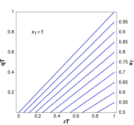
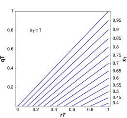
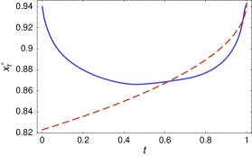
Figure 1: Isolines of the the limit xTsubscriptsuperscript𝑥𝑇x^{*}_{T} of the early exercise boundary at expiry T𝑇T of call option for the continuous arithmetic (left) and the continuous geometric average (right).

3.2 Integral equation for pricing Asian options

In this section we calculate the approximate formula for the American-style Asian option with various floating strike averages. The next lemma will be useful in calculations to follow.

Lemma 3.1

(?) Let ω=lnΩ𝒩(α,β2)𝜔Ωsimilar-to𝒩𝛼superscript𝛽2\omega=\ln{\Omega}\sim\mathcal{N}(\alpha,\beta^{2}) and define γα+β2lnKβ𝛾𝛼superscript𝛽2𝐾𝛽\gamma\equiv\frac{\alpha+\beta^{2}-\ln{K}}{\beta}, where K>0𝐾0K>0. We have

𝔼[1{ρΩρK}]=𝚽(ρ(γβ)),𝔼[1{ρΩρK}ΩlnΩ]=eα+β22((α+β2)𝚽(ργ)+ρβΦ(γ)),formulae-sequence𝔼delimited-[]subscript1𝜌Ω𝜌𝐾𝚽𝜌𝛾𝛽𝔼delimited-[]subscript1𝜌Ω𝜌𝐾ΩΩsuperscript𝑒𝛼superscript𝛽22𝛼superscript𝛽2𝚽𝜌𝛾𝜌𝛽𝛷𝛾\displaystyle\mathbb{E}\big{[}1_{\{\rho\Omega\geq\rho K\}}\big{]}={\bf\Phi}(\rho(\gamma-\beta)),\,\mathbb{E}\big{[}1_{\{\rho\Omega\geq\rho K\}}\Omega\ln{\Omega}\big{]}=e^{\alpha+\frac{\beta^{2}}{2}}\Big{(}(\alpha+\beta^{2}){\bf\Phi}(\rho\gamma)+\rho\beta{\it\Phi}(\gamma)\Big{)},
𝔼[1{ρΩρK}Ω]=eα+β22𝚽(ργ),𝔼[(ρ(ΩK))+]=ρ(eα+β22𝚽(ργ)K𝚽(ρ(γβ))),formulae-sequence𝔼delimited-[]subscript1𝜌Ω𝜌𝐾Ωsuperscript𝑒𝛼superscript𝛽22𝚽𝜌𝛾𝔼delimited-[]superscript𝜌Ω𝐾𝜌superscript𝑒𝛼superscript𝛽22𝚽𝜌𝛾𝐾𝚽𝜌𝛾𝛽\displaystyle\mathbb{E}\big{[}1_{\{\rho\Omega\geq\rho K\}}\Omega\big{]}=e^{\alpha+\frac{\beta^{2}}{2}}{\bf\Phi}(\rho\gamma),\,\mathbb{E}\big{[}(\rho(\Omega-K))^{+}\big{]}=\rho\Big{(}e^{\alpha+\frac{\beta^{2}}{2}}{\bf\Phi}(\rho\gamma)-K{\bf\Phi}(\rho(\gamma-\beta))\Big{)},

where ρ{1,1}𝜌11\rho\in\{-1,1\} and 𝚽()𝚽{\bf\Phi}(\cdot) and Φ()𝛷{\it\Phi}(\cdot) are standard normal cumulative distribution and density functions, resp.

3.2.1 Geometric average

In this section we recall the integral equation for pricing American-style of Asian geometrically averaged floating strike options. It was derived for the case q=0𝑞0q=0 by (?) and for the general case q0𝑞0q\geq 0 by (?).

Lemma 3.2

(?) In the case of geometric averaging, the variable xtg=AtgStsubscriptsuperscript𝑥𝑔𝑡superscriptsubscript𝐴𝑡𝑔subscript𝑆𝑡x^{g}_{t}=\frac{A_{t}^{g}}{S_{t}} has log-normal (conditioned) distribution lnxug|t𝒩(αt,u,βt,u2)similar-toconditionalsuperscriptsubscript𝑥𝑢𝑔subscript𝑡𝒩subscript𝛼𝑡𝑢subscriptsuperscript𝛽2𝑡𝑢\ln{x_{u}^{g}}|\mathcal{F}_{t}\sim\mathcal{N}(\alpha_{t,u},\beta^{2}_{t,u}), where ut𝑢𝑡u\geq t and parameters αt,u=α(t,u,xt)subscript𝛼𝑡𝑢𝛼𝑡𝑢subscript𝑥𝑡\alpha_{t,u}=\alpha(t,u,x_{t}) and βt,u=β(t,u)subscript𝛽𝑡𝑢𝛽𝑡𝑢\beta_{t,u}=\beta(t,u) are defined by

αt,ug=tulnxtgu2t22u(rq+σ22),βt,ug=σu3u3t3.formulae-sequencesubscriptsuperscript𝛼𝑔𝑡𝑢𝑡𝑢superscriptsubscript𝑥𝑡𝑔superscript𝑢2superscript𝑡22𝑢𝑟𝑞superscript𝜎22subscriptsuperscript𝛽𝑔𝑡𝑢𝜎𝑢3superscript𝑢3superscript𝑡3\alpha^{g}_{t,u}=\frac{t}{u}\ln{x_{t}^{g}}-\frac{u^{2}-t^{2}}{2u}(r-q+\frac{\sigma^{2}}{2}),\quad\beta^{g}_{t,u}=\frac{\sigma}{u\sqrt{3}}\sqrt{u^{3}-t^{3}}.

Now one can apply Lemma 3.1 in order to calculate the formula for option with the geometric averaging. Recall that for the floating strike Asian call or put option, the stopping region 𝒮={(t,x),x0,ρxt>ρx}\mathcal{S}=\{(t,x),x\geq 0,\rho x^{*}_{t}>\rho x\}, where xtsubscriptsuperscript𝑥𝑡x^{*}_{t} is the exercise boundary and ρ=1𝜌1\rho=1 for the case of a call option whereas ρ=1𝜌1\rho=-1 for a put option. If we insert the expression dAtgAtg𝑑subscriptsuperscript𝐴𝑔𝑡subscriptsuperscript𝐴𝑔𝑡\frac{dA^{g}_{t}}{A^{g}_{t}} for the geometric average (see Table 1) into (4) and (5) we obtain the formula for the European-style option

v~g(t,xt)superscript~𝑣𝑔𝑡subscript𝑥𝑡\displaystyle\widetilde{v}^{g}(t,x_{t}) =\displaystyle= 𝔼t𝒬[eqT(ρ(1xTg))+]=eqT𝔼t𝒬[(ρ(1xTg))+]superscriptsubscript𝔼𝑡𝒬delimited-[]superscript𝑒𝑞𝑇superscript𝜌1subscriptsuperscript𝑥𝑔𝑇superscript𝑒𝑞𝑇superscriptsubscript𝔼𝑡𝒬delimited-[]superscript𝜌1subscriptsuperscript𝑥𝑔𝑇\displaystyle\mathbb{E}_{t}^{\mathcal{Q}}\Big{[}e^{-qT}\Big{(}\rho(1-x^{g}_{T})\Big{)}^{+}\Big{]}=e^{-qT}\mathbb{E}_{t}^{\mathcal{Q}}\Big{[}\Big{(}\rho(1-x^{g}_{T})\Big{)}^{+}\Big{]}
=\displaystyle= ρeqT(𝚽(ρ(αt,Tgβt,Tg))eαt,Tg+(βt,Tg)22𝚽(ρ(αt,Tgβt,Tg+βt,Tg))).𝜌superscript𝑒𝑞𝑇𝚽𝜌subscriptsuperscript𝛼𝑔𝑡𝑇subscriptsuperscript𝛽𝑔𝑡𝑇superscript𝑒subscriptsuperscript𝛼𝑔𝑡𝑇superscriptsubscriptsuperscript𝛽𝑔𝑡𝑇22𝚽𝜌subscriptsuperscript𝛼𝑔𝑡𝑇subscriptsuperscript𝛽𝑔𝑡𝑇subscriptsuperscript𝛽𝑔𝑡𝑇\displaystyle\rho e^{-qT}\Bigg{(}{\bf\Phi}\Big{(}-\rho\Big{(}\frac{\alpha^{g}_{t,T}}{\beta^{g}_{t,T}}\Big{)}\Big{)}-e^{\alpha^{g}_{t,T}+\frac{(\beta^{g}_{t,T})^{2}}{2}}{\bf\Phi}\Big{(}-\rho\Big{(}\frac{\alpha^{g}_{t,T}}{\beta^{g}_{t,T}}+\beta^{g}_{t,T}\Big{)}\Big{)}\Bigg{)}.

and the value of the American early exercise bonus premium

e~g(t,xt)superscript~𝑒𝑔𝑡subscript𝑥𝑡\displaystyle\widetilde{e}^{g}(t,x_{t}) =\displaystyle= 𝔼t𝒬[tTρequxug𝟏𝒮(u,xug)(dAugAug(rq(xug)1)du)]superscriptsubscript𝔼𝑡𝒬delimited-[]superscriptsubscript𝑡𝑇𝜌superscript𝑒𝑞𝑢subscriptsuperscript𝑥𝑔𝑢subscript1𝒮𝑢subscriptsuperscript𝑥𝑔𝑢𝑑subscriptsuperscript𝐴𝑔𝑢subscriptsuperscript𝐴𝑔𝑢𝑟𝑞superscriptsubscriptsuperscript𝑥𝑔𝑢1𝑑𝑢\displaystyle\mathbb{E}_{t}^{\mathcal{Q}}\Big{[}\int_{t}^{T}{\rho e^{-qu}x^{g}_{u}{\bf 1}_{\mathcal{S}}(u,x^{g}_{u})\Big{(}\frac{dA^{g}_{u}}{A^{g}_{u}}-(r-q(x^{g}_{u})^{-1})du\Big{)}}\Big{]}
=\displaystyle= tTρequ𝔼t𝒬[𝟏{ρxu>ρxug}(1uxuglnxugrxug+q)]𝑑usuperscriptsubscript𝑡𝑇𝜌superscript𝑒𝑞𝑢superscriptsubscript𝔼𝑡𝒬delimited-[]subscript1𝜌subscriptsuperscript𝑥𝑢𝜌subscriptsuperscript𝑥𝑔𝑢1𝑢subscriptsuperscript𝑥𝑔𝑢subscriptsuperscript𝑥𝑔𝑢𝑟subscriptsuperscript𝑥𝑔𝑢𝑞differential-d𝑢\displaystyle\int_{t}^{T}{\rho e^{-qu}\mathbb{E}_{t}^{\mathcal{Q}}\Big{[}{\bf 1}_{\{\rho x^{*}_{u}>\rho x^{g}_{u}\}}\Big{(}-\frac{1}{u}x^{g}_{u}\ln{x^{g}_{u}}-rx^{g}_{u}+q\Big{)}\Big{]}}du
=\displaystyle= tTρequ(q𝚽(ρ(βt,ugγt,ug))\displaystyle\int_{t}^{T}{\rho e^{-qu}\Bigg{(}q{\bf\Phi}(\rho(\beta^{g}_{t,u}-\gamma^{g}_{t,u}))}
+eαt,ug+(βt,ug)22(ρβt,ugu𝚽(γt,ug)(r+αt,ug+(βt,ug)2u)𝚽(ργt,ug)))du,\displaystyle{+e^{\alpha^{g}_{t,u}+\frac{(\beta^{g}_{t,u})^{2}}{2}}\Bigg{(}\rho\frac{\beta^{g}_{t,u}}{u}{\bf\Phi}^{\prime}(\gamma^{g}_{t,u})-\Big{(}r+\frac{\alpha^{g}_{t,u}+(\beta^{g}_{t,u})^{2}}{u}\Big{)}{\bf\Phi}(-\rho\gamma^{g}_{t,u})\Bigg{)}\Bigg{)}}du,

where 𝚽()𝚽{\bf\Phi}(\cdot) is the standard normal cumulative distribution function and

γt,ug=αt,uglnxuβt,ug+βt,ug.subscriptsuperscript𝛾𝑔𝑡𝑢subscriptsuperscript𝛼𝑔𝑡𝑢subscriptsuperscript𝑥𝑢subscriptsuperscript𝛽𝑔𝑡𝑢subscriptsuperscript𝛽𝑔𝑡𝑢\gamma^{g}_{t,u}=\frac{\alpha^{g}_{t,u}-\ln{x^{*}_{u}}}{\beta^{g}_{t,u}}+\beta^{g}_{t,u}.

Returning to the original variables we obtain the formula of American-style floating strike Asian option with geometrically averaged floating strike:

Vg(t,S,A)=SeqtV~g(t,A/S)=Seqt(v~g(t,A/S)+e~g(t,A/S)).superscript𝑉𝑔𝑡𝑆𝐴𝑆superscript𝑒𝑞𝑡superscript~𝑉𝑔𝑡𝐴𝑆𝑆superscript𝑒𝑞𝑡superscript~𝑣𝑔𝑡𝐴𝑆superscript~𝑒𝑔𝑡𝐴𝑆V^{g}(t,S,A)=Se^{qt}\widetilde{V}^{g}(t,A/S)=Se^{qt}(\widetilde{v}^{g}(t,A/S)+\widetilde{e}^{g}(t,A/S)).

If we formally set value of the continuous dividend rate to zero, i.e. q=0𝑞0q=0, the result is identical to the expression obtained in the paper (?)).

3.2.2 Approximation for the arithmetic average

Unfortunately, in the case of an arithmetically averaged floating strike Asian option the probabilistic distribution function of the arithmetic average cannot be expressed in an explicit way. Following (?) we approximate the probabilistic distribution of the variable xta=AtaStsuperscriptsubscript𝑥𝑡𝑎superscriptsubscript𝐴𝑡𝑎subscript𝑆𝑡x_{t}^{a}=\frac{A_{t}^{a}}{S_{t}} for the continuous arithmetic average Atasuperscriptsubscript𝐴𝑡𝑎A_{t}^{a} by the log-normal conditioned distribution, i.e. lnxua|t𝒩(αt,ua,(βt,ua)2)similar-toconditionalsuperscriptsubscript𝑥𝑢𝑎subscript𝑡𝒩subscriptsuperscript𝛼𝑎𝑡𝑢superscriptsubscriptsuperscript𝛽𝑎𝑡𝑢2\ln{x_{u}^{a}}|\mathcal{F}_{t}\sim\mathcal{N}(\alpha^{a}_{t,u},(\beta^{a}_{t,u})^{2}) at time t𝑡t, where

αt,ua=2ln𝔼t𝒬[xua]12ln𝔼t𝒬[(xua)2],βt,ua=ln𝔼t𝒬[(xua)2]2ln𝔼t𝒬[xua].formulae-sequencesubscriptsuperscript𝛼𝑎𝑡𝑢2superscriptsubscript𝔼𝑡𝒬delimited-[]subscriptsuperscript𝑥𝑎𝑢12superscriptsubscript𝔼𝑡𝒬delimited-[]superscriptsubscriptsuperscript𝑥𝑎𝑢2subscriptsuperscript𝛽𝑎𝑡𝑢superscriptsubscript𝔼𝑡𝒬delimited-[]superscriptsubscriptsuperscript𝑥𝑎𝑢22superscriptsubscript𝔼𝑡𝒬delimited-[]subscriptsuperscript𝑥𝑎𝑢\alpha^{a}_{t,u}=2\ln{\mathbb{E}_{t}^{\mathcal{Q}}\big{[}x^{a}_{u}\big{]}}-\frac{1}{2}\ln{\mathbb{E}_{t}^{\mathcal{Q}}\big{[}(x^{a}_{u})^{2}\big{]}},\quad\beta^{a}_{t,u}=\sqrt{\ln{\mathbb{E}_{t}^{\mathcal{Q}}\big{[}(x^{a}_{u})^{2}\big{]}}-2\ln{\mathbb{E}_{t}^{\mathcal{Q}}\big{[}x^{a}_{u}\big{]}}}. (9)
Lemma 3.3

Consider the variable xu=AuSusubscript𝑥𝑢subscript𝐴𝑢subscript𝑆𝑢x_{u}=\frac{A_{u}}{S_{u}}, where Ausubscript𝐴𝑢A_{u} and Susubscript𝑆𝑢S_{u} are defined as the arithmetic average (see Table 1) and as in (2), resp. First two conditioned moments 𝔼t𝒬[xua]superscriptsubscript𝔼𝑡𝒬delimited-[]subscriptsuperscript𝑥𝑎𝑢\mathbb{E}_{t}^{\mathcal{Q}}\big{[}x^{a}_{u}\big{]} and 𝔼t𝒬[(xua)2]superscriptsubscript𝔼𝑡𝒬delimited-[]superscriptsubscriptsuperscript𝑥𝑎𝑢2\mathbb{E}_{t}^{\mathcal{Q}}\big{[}(x^{a}_{u})^{2}\big{]} of xusubscript𝑥𝑢x_{u} entering the expressions for the functions αt,ua=αa(t,u,xta)subscriptsuperscript𝛼𝑎𝑡𝑢superscript𝛼𝑎𝑡𝑢subscriptsuperscript𝑥𝑎𝑡\alpha^{a}_{t,u}=\alpha^{a}(t,u,x^{a}_{t}) and βt,ua=βa(t,u,xta)subscriptsuperscript𝛽𝑎𝑡𝑢superscript𝛽𝑎𝑡𝑢subscriptsuperscript𝑥𝑎𝑡\beta^{a}_{t,u}=\beta^{a}(t,u,x^{a}_{t}) can be calculated, for tu𝑡𝑢t\leq u, as follows:

𝔼t𝒬[xua]superscriptsubscript𝔼𝑡𝒬delimited-[]subscriptsuperscript𝑥𝑎𝑢\displaystyle\mathbb{E}_{t}^{\mathcal{Q}}\big{[}x^{a}_{u}\big{]} =\displaystyle= xtatue(rq)(ut)+1(rq)u(1e(rq)(ut)),subscriptsuperscript𝑥𝑎𝑡𝑡𝑢superscript𝑒𝑟𝑞𝑢𝑡1𝑟𝑞𝑢1superscript𝑒𝑟𝑞𝑢𝑡\displaystyle x^{a}_{t}\frac{t}{u}e^{-(r-q)(u-t)}+\frac{1}{(r-q)u}\big{(}1-e^{-(r-q)(u-t)}\big{)}, (10)
𝔼t𝒬[(xua)2]superscriptsubscript𝔼𝑡𝒬delimited-[]superscriptsubscriptsuperscript𝑥𝑎𝑢2\displaystyle\mathbb{E}_{t}^{\mathcal{Q}}\big{[}(x^{a}_{u})^{2}\big{]} =\displaystyle= (xta)2t2u2e2(rqσ22)(ut)+xta2te(rq)(ut)u2(rq)(1e(rq)(ut))superscriptsubscriptsuperscript𝑥𝑎𝑡2superscript𝑡2superscript𝑢2superscript𝑒2𝑟𝑞superscript𝜎22𝑢𝑡subscriptsuperscript𝑥𝑎𝑡2𝑡superscript𝑒𝑟𝑞𝑢𝑡superscript𝑢2𝑟𝑞1superscript𝑒𝑟𝑞𝑢𝑡\displaystyle(x^{a}_{t})^{2}\frac{t^{2}}{u^{2}}e^{-2(r-q-\frac{\sigma^{2}}{2})(u-t)}+x^{a}_{t}\frac{2te^{-(r-q)(u-t)}}{u^{2}(r-q)}\big{(}1-e^{-(r-q)(u-t)}\big{)}
+(rqσ2)2(rqσ22)e(rq)(ut)+(rq)e2(rqσ22)(ut)u2(rq)(rqσ22)(rqσ2).𝑟𝑞superscript𝜎22𝑟𝑞superscript𝜎22superscript𝑒𝑟𝑞𝑢𝑡𝑟𝑞superscript𝑒2𝑟𝑞superscript𝜎22𝑢𝑡superscript𝑢2𝑟𝑞𝑟𝑞superscript𝜎22𝑟𝑞superscript𝜎2\displaystyle+\frac{(r-q-\sigma^{2})-2(r-q-\frac{\sigma^{2}}{2})e^{-(r-q)(u-t)}+(r-q)e^{-2(r-q-\frac{\sigma^{2}}{2})(u-t)}}{u^{2}(r-q)(r-q-\frac{\sigma^{2}}{2})(r-q-\sigma^{2})}.

P r o o f: Following the lines of the derivation of 𝔼t𝒬[xua]superscriptsubscript𝔼𝑡𝒬delimited-[]subscriptsuperscript𝑥𝑎𝑢\mathbb{E}_{t}^{\mathcal{Q}}[x^{a}_{u}] from (?) adopted for a general dividend yield q0𝑞0q\geq 0 we obtain the first moment

𝔼t𝒬[xua]=xtatue(rq)(ut)+1e(rq)(ut)(rq)u.superscriptsubscript𝔼𝑡𝒬delimited-[]subscriptsuperscript𝑥𝑎𝑢subscriptsuperscript𝑥𝑎𝑡𝑡𝑢superscript𝑒𝑟𝑞𝑢𝑡1superscript𝑒𝑟𝑞𝑢𝑡𝑟𝑞𝑢\mathbb{E}_{t}^{\mathcal{Q}}\Big{[}x^{a}_{u}\Big{]}=x^{a}_{t}\frac{t}{u}e^{-(r-q)(u-t)}+\frac{1-e^{-(r-q)(u-t)}}{(r-q)u}.

Although we follow the proof by (?), we have to make a slight correction in the derivation of the second conditioned moment. Using the definition of Stsubscript𝑆𝑡S_{t}, we have, for all v[t,u]𝑣𝑡𝑢v\in[t,u],

𝔼t𝒬[SvSu]=𝔼t𝒬[e(rq+σ22)(vu)+σ(Wv𝒬Wu𝒬)]=e(rq+σ22)(vu)+σ22|vu|=e(rq)(vu).superscriptsubscript𝔼𝑡𝒬delimited-[]subscript𝑆𝑣subscript𝑆𝑢superscriptsubscript𝔼𝑡𝒬delimited-[]superscript𝑒𝑟𝑞superscript𝜎22𝑣𝑢𝜎superscriptsubscript𝑊𝑣𝒬superscriptsubscript𝑊𝑢𝒬superscript𝑒𝑟𝑞superscript𝜎22𝑣𝑢superscript𝜎22𝑣𝑢superscript𝑒𝑟𝑞𝑣𝑢\mathbb{E}_{t}^{\mathcal{Q}}\Big{[}\frac{S_{v}}{S_{u}}\Big{]}=\mathbb{E}_{t}^{\mathcal{Q}}\Big{[}e^{(r-q+\frac{\sigma^{2}}{2})(v-u)+\sigma(W_{v}^{\mathcal{Q}}-W_{u}^{\mathcal{Q}})}\Big{]}=e^{(r-q+\frac{\sigma^{2}}{2})(v-u)+\frac{\sigma^{2}}{2}|v-u|}=e^{(r-q)(v-u)}.

We need to simplify the expression for the the second conditioned moment

𝔼t𝒬[(xua)2]=𝔼t𝒬[(1u0uSvSu𝑑v)2]superscriptsubscript𝔼𝑡𝒬delimited-[]superscriptsubscriptsuperscript𝑥𝑎𝑢2superscriptsubscript𝔼𝑡𝒬delimited-[]superscript1𝑢superscriptsubscript0𝑢subscript𝑆𝑣subscript𝑆𝑢differential-d𝑣2\displaystyle\mathbb{E}_{t}^{\mathcal{Q}}\Big{[}(x^{a}_{u})^{2}\Big{]}=\mathbb{E}_{t}^{\mathcal{Q}}\Big{[}\Big{(}\frac{1}{u}\int_{0}^{u}{\frac{S_{v}}{S_{u}}}dv\Big{)}^{2}\Big{]}
=\displaystyle= (xta)2t2u2𝔼t𝒬[StSuStSu]+2xttu2𝔼t𝒬[StSu]tu𝔼t𝒬[SvSu]𝑑v+1u2tutu𝔼t𝒬[SzSuSvSu]𝑑v𝑑z.superscriptsubscriptsuperscript𝑥𝑎𝑡2superscript𝑡2superscript𝑢2superscriptsubscript𝔼𝑡𝒬delimited-[]subscript𝑆𝑡subscript𝑆𝑢subscript𝑆𝑡subscript𝑆𝑢2subscript𝑥𝑡𝑡superscript𝑢2superscriptsubscript𝔼𝑡𝒬delimited-[]subscript𝑆𝑡subscript𝑆𝑢superscriptsubscript𝑡𝑢superscriptsubscript𝔼𝑡𝒬delimited-[]subscript𝑆𝑣subscript𝑆𝑢differential-d𝑣1superscript𝑢2superscriptsubscript𝑡𝑢superscriptsubscript𝑡𝑢superscriptsubscript𝔼𝑡𝒬delimited-[]subscript𝑆𝑧subscript𝑆𝑢subscript𝑆𝑣subscript𝑆𝑢differential-d𝑣differential-d𝑧\displaystyle(x^{a}_{t})^{2}\frac{t^{2}}{u^{2}}\mathbb{E}_{t}^{\mathcal{Q}}\Big{[}\frac{S_{t}}{S_{u}}\frac{S_{t}}{S_{u}}\Big{]}+2x_{t}\frac{t}{u^{2}}\mathbb{E}_{t}^{\mathcal{Q}}\Big{[}\frac{S_{t}}{S_{u}}\Big{]}\int_{t}^{u}{\mathbb{E}_{t}^{\mathcal{Q}}\Big{[}\frac{S_{v}}{S_{u}}\Big{]}}dv+\frac{1}{u^{2}}\int_{t}^{u}\int_{t}^{u}{\mathbb{E}_{t}^{\mathcal{Q}}\Big{[}\frac{S_{z}}{S_{u}}\frac{S_{v}}{S_{u}}\Big{]}}dv\ dz.

Assuming that uz,v𝑢𝑧𝑣u\geq z,v and let m=min{z,v}𝑚𝑧𝑣m=\min{\{z,v\}} and M=max{z,v}𝑀𝑧𝑣M=\max{\{z,v\}}, we have

e(rq+σ22)(z+v2u)SzSuSvSusuperscript𝑒𝑟𝑞superscript𝜎22𝑧𝑣2𝑢subscript𝑆𝑧subscript𝑆𝑢subscript𝑆𝑣subscript𝑆𝑢\displaystyle e^{-(r-q+\frac{\sigma^{2}}{2})(z+v-2u)}\frac{S_{z}}{S_{u}}\frac{S_{v}}{S_{u}} =\displaystyle= eσ(Wz𝒬+Wv𝒬2Wu𝒬)=eσ(2(Wu𝒬WM𝒬)+(WM𝒬Wm𝒬)),superscript𝑒𝜎superscriptsubscript𝑊𝑧𝒬superscriptsubscript𝑊𝑣𝒬2superscriptsubscript𝑊𝑢𝒬superscript𝑒𝜎2superscriptsubscript𝑊𝑢𝒬superscriptsubscript𝑊𝑀𝒬superscriptsubscript𝑊𝑀𝒬superscriptsubscript𝑊𝑚𝒬\displaystyle e^{\sigma(W_{z}^{\mathcal{Q}}+W_{v}^{\mathcal{Q}}-2W_{u}^{\mathcal{Q}})}=e^{-\sigma(2(W_{u}^{\mathcal{Q}}-W_{M}^{\mathcal{Q}})+(W_{M}^{\mathcal{Q}}-W_{m}^{\mathcal{Q}}))},
𝔼t𝒬[SzSuSvSu]superscriptsubscript𝔼𝑡𝒬delimited-[]subscript𝑆𝑧subscript𝑆𝑢subscript𝑆𝑣subscript𝑆𝑢\displaystyle\mathbb{E}_{t}^{\mathcal{Q}}\Big{[}\frac{S_{z}}{S_{u}}\frac{S_{v}}{S_{u}}\Big{]} =\displaystyle= e(rq)(z+v2u)+σ2(uM).superscript𝑒𝑟𝑞𝑧𝑣2𝑢superscript𝜎2𝑢𝑀\displaystyle e^{(r-q)(z+v-2u)+\sigma^{2}(u-M)}.

We have calculated all expressions we need to evaluate the second conditioned moment. If we put all together and perform necessary calculation we obtain (3.3) and the proof of lemma follows. \square

Remark 3.2

If we formally set the value of the continuous dividend rate q=0𝑞0q=0 in Lemma 3.3 we obtain almost identical expression to that of (?) except of the second moment 𝔼t𝒬[(xua)2]superscriptsubscript𝔼𝑡𝒬delimited-[]superscriptsubscriptsuperscript𝑥𝑎𝑢2\mathbb{E}_{t}^{\mathcal{Q}}\Big{[}(x^{a}_{u})^{2}\Big{]} entering (9). The expression

𝔼t𝒬[(xua)2]HJsuperscriptsubscript𝔼𝑡𝒬subscriptdelimited-[]superscriptsubscriptsuperscript𝑥𝑎𝑢2𝐻𝐽\displaystyle\mathbb{E}_{t}^{\mathcal{Q}}\big{[}(x^{a}_{u})^{2}\big{]}_{HJ} =\displaystyle= (xta)2t2u2e2(rσ22)(ut)+xta2ter(ut)u2(rσ2)(1e(rσ2)(ut))superscriptsubscriptsuperscript𝑥𝑎𝑡2superscript𝑡2superscript𝑢2superscript𝑒2𝑟superscript𝜎22𝑢𝑡subscriptsuperscript𝑥𝑎𝑡2𝑡superscript𝑒𝑟𝑢𝑡superscript𝑢2𝑟superscript𝜎21superscript𝑒𝑟superscript𝜎2𝑢𝑡\displaystyle(x^{a}_{t})^{2}\frac{t^{2}}{u^{2}}e^{-2(r-\frac{\sigma^{2}}{2})(u-t)}+x^{a}_{t}\frac{2te^{-r(u-t)}}{u^{2}(r-\sigma^{2})}\big{(}1-e^{-(r-\sigma^{2})(u-t)}\big{)}
+(rσ2)2(rσ22)er(ut)+re2(rσ22)(ut)u2r(rσ22)(rσ2).𝑟superscript𝜎22𝑟superscript𝜎22superscript𝑒𝑟𝑢𝑡𝑟superscript𝑒2𝑟superscript𝜎22𝑢𝑡superscript𝑢2𝑟𝑟superscript𝜎22𝑟superscript𝜎2\displaystyle+\frac{(r-\sigma^{2})-2(r-\frac{\sigma^{2}}{2})e^{-r(u-t)}+re^{-2(r-\frac{\sigma^{2}}{2})(u-t)}}{u^{2}r(r-\frac{\sigma^{2}}{2})(r-\sigma^{2})}.

by (?) differs from our (3.3) in the second summand where the term rσ2𝑟superscript𝜎2r-\sigma^{2} is replaced by r𝑟r in both in the denominator and exponent.

Now we can return to the problem of valuation of an Asian option. First we replace the general form of the average in (5) by the expression for the arithmetic average defined as arithmetic average in Table 1. The stopping region 𝒮𝒮\mathcal{S} is the same as for the case of geometric averaging.

Using Lemma 3.1 we calculate the value of both (4) and (5). The European part of the option has value

v~a(t,x)superscript~𝑣𝑎𝑡𝑥\displaystyle\widetilde{v}^{a}(t,x) =\displaystyle= 𝔼t𝒬[eqT(ρ(1xTa))+]superscriptsubscript𝔼𝑡𝒬delimited-[]superscript𝑒𝑞𝑇superscript𝜌1subscriptsuperscript𝑥𝑎𝑇\displaystyle\mathbb{E}_{t}^{\mathcal{Q}}\Big{[}e^{-qT}\Big{(}\rho(1-x^{a}_{T})\Big{)}^{+}\Big{]}
=\displaystyle= ρeqT(𝚽(ρ(αt,Taβt,Ta))eαt,Ta+(βt,Ta)22𝚽(ρ(αt,Taβt,Ta+βt,Ta)))𝜌superscript𝑒𝑞𝑇𝚽𝜌subscriptsuperscript𝛼𝑎𝑡𝑇subscriptsuperscript𝛽𝑎𝑡𝑇superscript𝑒subscriptsuperscript𝛼𝑎𝑡𝑇superscriptsubscriptsuperscript𝛽𝑎𝑡𝑇22𝚽𝜌subscriptsuperscript𝛼𝑎𝑡𝑇subscriptsuperscript𝛽𝑎𝑡𝑇subscriptsuperscript𝛽𝑎𝑡𝑇\displaystyle\rho e^{-qT}\Bigg{(}{\bf\Phi}\Big{(}-\rho\Big{(}\frac{\alpha^{a}_{t,T}}{\beta^{a}_{t,T}}\Big{)}\Big{)}-e^{\alpha^{a}_{t,T}+\frac{(\beta^{a}_{t,T})^{2}}{2}}{\bf\Phi}\Big{(}-\rho\Big{(}\frac{\alpha^{a}_{t,T}}{\beta^{a}_{t,T}}+\beta^{a}_{t,T}\Big{)}\Big{)}\Bigg{)}

and the American early exercise bonus premium

e~a(t,x)superscript~𝑒𝑎𝑡𝑥\displaystyle\widetilde{e}^{a}(t,x) =\displaystyle= 𝔼t𝒬[tTρequxua𝟏𝒮(u,xua)(dAuaAua(rq(xua)1)du)]superscriptsubscript𝔼𝑡𝒬delimited-[]superscriptsubscript𝑡𝑇𝜌superscript𝑒𝑞𝑢subscriptsuperscript𝑥𝑎𝑢subscript1𝒮𝑢subscriptsuperscript𝑥𝑎𝑢𝑑subscriptsuperscript𝐴𝑎𝑢subscriptsuperscript𝐴𝑎𝑢𝑟𝑞superscriptsubscriptsuperscript𝑥𝑎𝑢1𝑑𝑢\displaystyle\mathbb{E}_{t}^{\mathcal{Q}}\Big{[}\int_{t}^{T}{\rho e^{-qu}x^{a}_{u}{\bf 1}_{\mathcal{S}}(u,x^{a}_{u})\Big{(}\frac{dA^{a}_{u}}{A^{a}_{u}}-(r-q(x^{a}_{u})^{-1})du\Big{)}}\Big{]}
=\displaystyle= tTρequ𝔼t𝒬[1{ρxu>ρxua}(1u(1xua)rxua+q)]𝑑usuperscriptsubscript𝑡𝑇𝜌superscript𝑒𝑞𝑢superscriptsubscript𝔼𝑡𝒬delimited-[]subscript1𝜌subscriptsuperscript𝑥𝑢𝜌subscriptsuperscript𝑥𝑎𝑢1𝑢1subscriptsuperscript𝑥𝑎𝑢𝑟subscriptsuperscript𝑥𝑎𝑢𝑞differential-d𝑢\displaystyle\int_{t}^{T}{\rho e^{-qu}\mathbb{E}_{t}^{\mathcal{Q}}\Big{[}1_{\{\rho x^{*}_{u}>\rho x^{a}_{u}\}}\Big{(}\frac{1}{u}(1-x^{a}_{u})-rx^{a}_{u}+q\Big{)}\Big{]}}du
=\displaystyle= tTρequ((q+1u)𝚽(ρ(βt,uaγt,ua))(r+1u)eαt,ua+(βt,ua)22𝚽(ργt,ua))𝑑u,superscriptsubscript𝑡𝑇𝜌superscript𝑒𝑞𝑢𝑞1𝑢𝚽𝜌subscriptsuperscript𝛽𝑎𝑡𝑢subscriptsuperscript𝛾𝑎𝑡𝑢𝑟1𝑢superscript𝑒subscriptsuperscript𝛼𝑎𝑡𝑢superscriptsubscriptsuperscript𝛽𝑎𝑡𝑢22𝚽𝜌subscriptsuperscript𝛾𝑎𝑡𝑢differential-d𝑢\displaystyle\int_{t}^{T}{\rho e^{-qu}\Bigg{(}\Big{(}q+\frac{1}{u}\Big{)}{\bf\Phi}(\rho(\beta^{a}_{t,u}-\gamma^{a}_{t,u}))-\Big{(}r+\frac{1}{u}\Big{)}e^{\alpha^{a}_{t,u}+\frac{(\beta^{a}_{t,u})^{2}}{2}}{\bf\Phi}(-\rho\gamma^{a}_{t,u})\Bigg{)}}du,

where 𝚽()𝚽{\bf\Phi}(\cdot) is the standard normal cumulative distribution function and

γt,ua=αt,ualnxuβt,ua+βt,ua.subscriptsuperscript𝛾𝑎𝑡𝑢subscriptsuperscript𝛼𝑎𝑡𝑢subscriptsuperscript𝑥𝑢subscriptsuperscript𝛽𝑎𝑡𝑢subscriptsuperscript𝛽𝑎𝑡𝑢\gamma^{a}_{t,u}=\frac{\alpha^{a}_{t,u}-\ln{x^{*}_{u}}}{\beta^{a}_{t,u}}+\beta^{a}_{t,u}.

Returning to the original variables we have the approximate value of American-style Asian option with a continuous arithmetic averaging

Va(t,S,A)=SeqtV~a(t,x)=Seqt(v~a(t,x)+e~a(t,x)).superscript𝑉𝑎𝑡𝑆𝐴𝑆superscript𝑒𝑞𝑡superscript~𝑉𝑎𝑡𝑥𝑆superscript𝑒𝑞𝑡superscript~𝑣𝑎𝑡𝑥superscript~𝑒𝑎𝑡𝑥V^{a}(t,S,A)=Se^{qt}\widetilde{V}^{a}(t,x)=Se^{qt}(\widetilde{v}^{a}(t,x)+\widetilde{e}^{a}(t,x)).

3.3 Expansion of the early exercise boundary close to expiry

Throughout this section we shall assume the structural assumption on the interest and dividend rates:

r>q0.𝑟𝑞0r>q\geq 0. (12)

We shall calculate an approximation of the call option early exercise boundary function for a call option. The approximation is obtained by the first order Taylor series expansion in the τ𝜏\sqrt{\tau} variable, where τ=Tt𝜏𝑇𝑡\tau=T-t is the time to expiry. To approximate the early exercise boundary function by the Taylor expansion, we need to calculate the first derivative of xtsubscriptsuperscript𝑥𝑡x^{*}_{t} at expiry T𝑇T with respect to Tt𝑇𝑡\sqrt{T-t} variable. Following (???) we propose an approximation of the early exercise boundary xtsubscriptsuperscript𝑥𝑡x^{*}_{t} in the form

xt=xT(1+CTt)+O(Tt)astT,formulae-sequencesubscriptsuperscript𝑥𝑡subscriptsuperscript𝑥𝑇1𝐶𝑇𝑡𝑂𝑇𝑡as𝑡𝑇x^{*}_{t}=x^{*}_{T}(1+C\sqrt{T-t})+O(T-t)\quad\hbox{as}\ t\to T,

where C𝐶C\in\mathbb{R} is a constant. To calculate C𝐶C, we use the condition of smoothness of the early exercise boundary of the call option across the early exercise boundary - smooth pasting principle (c.f. (??)). Since V~(T,x)=eqT(1x)+~𝑉𝑇𝑥superscript𝑒𝑞𝑇superscript1𝑥\widetilde{V}(T,x)=e^{-qT}(1-x)^{+} we have

1=eqtV~x(t,xt)=eqtv~tx(t,xt)+eqte~tx(t,xt)=v^x(t,xt)+tTe^Ix(t,xt,u,xu)𝑑u.1superscript𝑒𝑞𝑡~𝑉𝑥𝑡superscriptsubscript𝑥𝑡superscript𝑒𝑞𝑡subscript~𝑣𝑡𝑥𝑡superscriptsubscript𝑥𝑡superscript𝑒𝑞𝑡subscript~𝑒𝑡𝑥𝑡superscriptsubscript𝑥𝑡subscript^𝑣𝑥𝑡superscriptsubscript𝑥𝑡superscriptsubscript𝑡𝑇subscript^𝑒𝐼𝑥𝑡superscriptsubscript𝑥𝑡𝑢superscriptsubscript𝑥𝑢differential-d𝑢-1=e^{qt}\frac{\partial\widetilde{V}}{\partial x}(t,x_{t}^{*})=e^{qt}\frac{\partial\widetilde{v}_{t}}{\partial x}(t,x_{t}^{*})+e^{qt}\frac{\partial\widetilde{e}_{t}}{\partial x}(t,x_{t}^{*})=\widehat{v}_{x}(t,x_{t}^{*})+\int_{t}^{T}{\widehat{e}_{Ix}(t,x_{t}^{*},u,x_{u}^{*})}\ du. (13)

In further derivation we use following limits (according to the Lemma 3.2, Lemma 3.3 and Table 3). We recall that αt,u=α(t,u,x)subscript𝛼𝑡𝑢𝛼𝑡𝑢𝑥\alpha_{t,u}=\alpha(t,u,x), βt,ua=βa(t,u,xa)subscriptsuperscript𝛽𝑎𝑡𝑢superscript𝛽𝑎𝑡𝑢superscript𝑥𝑎\beta^{a}_{t,u}=\beta^{a}(t,u,x^{a}) and βt,ug=βg(t,u)subscriptsuperscript𝛽𝑔𝑡𝑢superscript𝛽𝑔𝑡𝑢\beta^{g}_{t,u}=\beta^{g}(t,u).

limτ0αTτ,T=limτ0αTτ,Tτ(1θ)subscript𝜏0subscript𝛼𝑇𝜏𝑇subscript𝜏0subscript𝛼𝑇𝜏𝑇𝜏1𝜃\displaystyle\lim_{\tau\rightarrow 0}\alpha_{T-\tau,T}=\lim_{\tau\rightarrow 0}\alpha_{T-\tau,T-\tau(1-\theta)} =\displaystyle= αT,T=lnxT<0,subscript𝛼𝑇𝑇superscriptsubscript𝑥𝑇0\displaystyle\alpha_{T,T}=\ln{x_{T}^{*}}<0,
limτ0βTτ,T=limτ0βTτ,Tτ(1θ)subscript𝜏0subscript𝛽𝑇𝜏𝑇subscript𝜏0subscript𝛽𝑇𝜏𝑇𝜏1𝜃\displaystyle\lim_{\tau\rightarrow 0}\beta_{T-\tau,T}=\lim_{\tau\rightarrow 0}\beta_{T-\tau,T-\tau(1-\theta)} =\displaystyle= βT,T=0+,subscript𝛽𝑇𝑇superscript0\displaystyle\beta_{T,T}=0^{+},
limτ0𝚽(αTτ,TβTτ,T)subscript𝜏0𝚽subscript𝛼𝑇𝜏𝑇subscript𝛽𝑇𝜏𝑇\displaystyle\lim_{\tau\rightarrow 0}{\bf\Phi}\Big{(}-\frac{\alpha_{T-\tau,T}}{\beta_{T-\tau,T}}\Big{)} =\displaystyle= 𝚽(lnxT0+)=1,𝚽superscriptsubscript𝑥𝑇superscript01\displaystyle{\bf\Phi}\Big{(}-\frac{\ln{x_{T}^{*}}}{0^{+}}\Big{)}=1,
limτ0𝚽(αTτ,TβTτ,T)(βTτ,T)nsubscript𝜏0superscript𝚽subscript𝛼𝑇𝜏𝑇subscript𝛽𝑇𝜏𝑇superscriptsubscript𝛽𝑇𝜏𝑇𝑛\displaystyle\lim_{\tau\rightarrow 0}\frac{{\bf\Phi}^{\prime}\Big{(}-\frac{\alpha_{T-\tau,T}}{\beta_{T-\tau,T}}\Big{)}}{(\beta_{T-\tau,T})^{n}} =\displaystyle= 0,0\displaystyle 0, (14)
limτ0lnxT(1+hστ(1θ))αTτ,Tτ(1θ)βTτ,Tτ(1θ)subscript𝜏0superscriptsubscript𝑥𝑇1𝜎𝜏1𝜃subscript𝛼𝑇𝜏𝑇𝜏1𝜃subscript𝛽𝑇𝜏𝑇𝜏1𝜃\displaystyle\lim_{\tau\rightarrow 0}\frac{\ln{x_{T}^{*}(1+h\sigma\sqrt{\tau(1-\theta)})}-\alpha_{T-\tau,T-\tau(1-\theta)}}{\beta_{T-\tau,T-\tau(1-\theta)}} =\displaystyle= h11θθ,11𝜃𝜃\displaystyle-h\frac{1-\sqrt{1-\theta}}{\sqrt{\theta}},
limτ0xαTτ,T=limτ0xαTτ,Tτ(1θ)subscript𝜏0subscript𝑥subscript𝛼𝑇𝜏𝑇subscript𝜏0subscript𝑥subscript𝛼𝑇𝜏𝑇𝜏1𝜃\displaystyle\lim_{\tau\rightarrow 0}\partial_{x}\alpha_{T-\tau,T}=\lim_{\tau\rightarrow 0}\partial_{x}\alpha_{T-\tau,T-\tau(1-\theta)} =\displaystyle= 1xT,1superscriptsubscript𝑥𝑇\displaystyle\frac{1}{x_{T}^{*}},
limτ0βTτ,TτβTτ,Tsubscript𝜏0subscript𝛽𝑇𝜏𝑇subscript𝜏subscript𝛽𝑇𝜏𝑇\displaystyle\lim_{\tau\rightarrow 0}\beta_{T-\tau,T}\,\partial_{\tau}\beta_{T-\tau,T} =\displaystyle= σ22.superscript𝜎22\displaystyle\frac{\sigma^{2}}{2}.

Since we have assumed r>q0𝑟𝑞0r>q\geq 0 we have 0<xT<10superscriptsubscript𝑥𝑇10<x_{T}^{*}<1 (see Table 3). Notice that both α𝛼\alpha and β𝛽\beta have polynomial order in τ𝜏\tau and the derivative of the normal cumulative distribution function (i.e. the probability density function) has exponential order in τ𝜏\tau variable. In both derivations we have used several properties of the derivative of normal cumulative distribution function 𝚽(x)𝚽𝑥{\bf\Phi}(x), e.g. 𝚽(x)=𝚽(x)superscript𝚽𝑥superscript𝚽𝑥{\bf\Phi}^{\prime}(x)={\bf\Phi}^{\prime}(-x), 𝚽′′(x)=x𝚽(x)superscript𝚽′′𝑥𝑥superscript𝚽𝑥{\bf\Phi}^{\prime\prime}(x)=-x{\bf\Phi}^{\prime}(x) and 𝚽(ab+b)=eab22𝚽(ab)superscript𝚽𝑎𝑏𝑏superscript𝑒𝑎superscript𝑏22superscript𝚽𝑎𝑏{\bf\Phi}^{\prime}(\frac{a}{b}+b)=e^{-a-\frac{b^{2}}{2}}{\bf\Phi}^{\prime}(\frac{a}{b}).

The following lemma will be useful in derivation of asymptotic behavior of the early exercise. Its proof is straightforward and follows from monotonicity of the right-hand side of equation (15) in the hh variable.

Lemma 3.4

The implicit equation

0=101𝚽(h11θθ)𝑑θ+h011θθ𝚽(h11θθ)𝑑θ01superscriptsubscript01𝚽11𝜃𝜃differential-d𝜃superscriptsubscript011𝜃𝜃superscript𝚽11𝜃𝜃differential-d𝜃0=1-\int_{0}^{1}{{\bf\Phi}\Big{(}-h\frac{1-\sqrt{1-\theta}}{\sqrt{\theta}}\Big{)}}d\theta+h\int_{0}^{1}{\frac{\sqrt{1-\theta}}{\sqrt{\theta}}{\bf\Phi}^{\prime}\Big{(}-h\frac{1-\sqrt{1-\theta}}{\sqrt{\theta}}\Big{)}}d\theta (15)

has the unique solution hsuperscripth^{*} having its approximate value h0.638833approaches-limitsuperscript0.638833h^{*}\doteq-0.638833.

Notice that the first order asymptotic expansion as tT𝑡𝑇t\to T of the early exercise boundary Sf(t)Sf(T)(1+0.638833σTt)subscript𝑆𝑓𝑡subscript𝑆𝑓𝑇10.638833𝜎𝑇𝑡S_{f}(t)\approx S_{f}(T)(1+0.638833\,\sigma\sqrt{T-t}) for the American call option derived by (??) contains the same constant h0.638833approaches-limitsuperscript0.638833-h^{*}\doteq 0.638833 where hsuperscripth^{*} is a solution of (15).

Remark 3.3

For the early exercise boundary function xt=xt(T,r,q,σ2)subscriptsuperscript𝑥𝑡subscriptsuperscript𝑥𝑡𝑇𝑟𝑞superscript𝜎2x^{*}_{t}=x^{*}_{t}(T,r,q,\sigma^{2}) as a function of the model parameters T,r,σ2>0,q0,formulae-sequence𝑇𝑟superscript𝜎20𝑞0T,r,\sigma^{2}>0,q\geq 0, we have the following scaling property:

xt(T,r,q,σ2)=xtT(1,rT,qT,σ2T).subscriptsuperscript𝑥𝑡𝑇𝑟𝑞superscript𝜎2subscriptsuperscript𝑥𝑡𝑇1𝑟𝑇𝑞𝑇superscript𝜎2𝑇x^{*}_{t}(T,r,q,\sigma^{2})=x^{*}_{\frac{t}{T}}(1,rT,qT,\sigma^{2}T).

3.3.1 Geometric average

We calculate the derivative of the European part of the expression (for the call option). Recall that α𝛼\alpha depends on the variable x𝑥x, but β𝛽\beta does not depend on this variable.

v^xg(t,x)=eqtxv~g(t,x)=eq(Tt)eαt,Tg+(βt,Tg)22𝚽(αt,Tgβt,Tgβt,Tg)αt,Tgx.superscriptsubscript^𝑣𝑥𝑔𝑡𝑥superscript𝑒𝑞𝑡𝑥superscript~𝑣𝑔𝑡𝑥superscript𝑒𝑞𝑇𝑡superscript𝑒subscriptsuperscript𝛼𝑔𝑡𝑇superscriptsubscriptsuperscript𝛽𝑔𝑡𝑇22𝚽subscriptsuperscript𝛼𝑔𝑡𝑇subscriptsuperscript𝛽𝑔𝑡𝑇subscriptsuperscript𝛽𝑔𝑡𝑇subscriptsuperscript𝛼𝑔𝑡𝑇𝑥\widehat{v}_{x}^{g}(t,x)=e^{qt}\frac{\partial}{\partial x}\widetilde{v}^{g}(t,x)=-e^{-q(T-t)}e^{\alpha^{g}_{t,T}+\frac{(\beta^{g}_{t,T})^{2}}{2}}{\bf\Phi}\Big{(}-\frac{\alpha^{g}_{t,T}}{\beta^{g}_{t,T}}-\beta^{g}_{t,T}\Big{)}\frac{\partial\alpha^{g}_{t,T}}{\partial x}.

Now we calculate the derivative of the integral function of American-style option bonus:

e^Ixg(t,x,u,xu)=eq(ut)1u((qu+xuru+xulnxu+xu(βt,ug)2βt,ug)𝚽(lnxuαt,ugβt,ug)\displaystyle\widehat{e}^{g}_{Ix}(t,x,u,x_{u}^{*})=e^{-q(u-t)}\frac{1}{u}\Bigg{(}\Big{(}\frac{-qu+x^{*}_{u}ru+x^{*}_{u}\ln{x^{*}_{u}}+x^{*}_{u}(\beta^{g}_{t,u})^{2}}{\beta^{g}_{t,u}}\Big{)}{\bf\Phi}^{\prime}\Big{(}\frac{\ln{x^{*}_{u}}-\alpha^{g}_{t,u}}{\beta^{g}_{t,u}}\Big{)}
eαt,ug+(βt,ug)22(ru+αt,ug+(βt,ug)2+1)𝚽(lnxuαt,ugβt,ugβt,ug))αt,ugx.\displaystyle-e^{\alpha^{g}_{t,u}+\frac{(\beta^{g}_{t,u})^{2}}{2}}\Big{(}ru+\alpha^{g}_{t,u}+(\beta^{g}_{t,u})^{2}+1\Big{)}{\bf\Phi}\Big{(}\frac{\ln{x^{*}_{u}}-\alpha^{g}_{t,u}}{\beta^{g}_{t,u}}-\beta^{g}_{t,u}\Big{)}\Bigg{)}\frac{\partial\alpha^{g}_{t,u}}{\partial x}.

We want to determine the behavior of the early exercise boundary near the expiry T𝑇T. The limit in the expression (13) leads to the trivial identity. By rearranging all of elements on the right side of the equation, we have an expression of order Tt𝑇𝑡T-t. We substitute τ=Tt𝜏𝑇𝑡\tau=T-t and xT=Gsubscriptsuperscript𝑥𝑇𝐺x^{*}_{T}=G and divide the equation by τ𝜏\tau. We have:

limτ01+v^x(Tτ,G(1+hστ))τ=limτ0v^xτ(Tτ,G(1+hστ)).subscript𝜏01subscript^𝑣𝑥𝑇𝜏𝐺1𝜎𝜏𝜏subscript𝜏0subscript^𝑣𝑥𝜏𝑇𝜏𝐺1𝜎𝜏\lim_{\tau\rightarrow 0}\frac{1+\widehat{v}_{x}(T-\tau,G(1+h\sigma\sqrt{\tau}))}{\tau}=\lim_{\tau\rightarrow 0}\frac{\partial\widehat{v}_{x}}{\partial\tau}(T-\tau,G(1+h\sigma\sqrt{\tau})).

According to the Lemma 3.2 and Table 3 we have:

limτ0ταTτ,TgxαTτ,Tg+x,τ2αTτ,Tg=1G(qqG1Tσ22).subscript𝜏0subscript𝜏subscriptsuperscript𝛼𝑔𝑇𝜏𝑇subscript𝑥subscriptsuperscript𝛼𝑔𝑇𝜏𝑇subscriptsuperscript2𝑥𝜏subscriptsuperscript𝛼𝑔𝑇𝜏𝑇1𝐺𝑞𝑞𝐺1𝑇superscript𝜎22\lim_{\tau\rightarrow 0}\partial_{\tau}\alpha^{g}_{T-\tau,T}\,\partial_{x}\alpha^{g}_{T-\tau,T}+\partial^{2}_{x,\tau}\alpha^{g}_{T-\tau,T}=\frac{1}{G}\Big{(}q-\frac{q}{G}-\frac{1}{T}-\frac{\sigma^{2}}{2}\Big{)}.

The only non-zero elements of the first partial limit are the elements multiplied by the cumulative distribution function.

limτ01+v^x(Tτ,G(1+hστ))τ=limτ0τ(1eqτeαTτ,Tg+(βTτ,Tg)22αTτ,Tgx)=qG+1T.subscript𝜏01subscript^𝑣𝑥𝑇𝜏𝐺1𝜎𝜏𝜏subscript𝜏0𝜏1superscript𝑒𝑞𝜏superscript𝑒subscriptsuperscript𝛼𝑔𝑇𝜏𝑇superscriptsubscriptsuperscript𝛽𝑔𝑇𝜏𝑇22subscriptsuperscript𝛼𝑔𝑇𝜏𝑇𝑥𝑞𝐺1𝑇\lim_{\tau\rightarrow 0}\frac{1+\widehat{v}_{x}(T-\tau,G(1+h\sigma\sqrt{\tau}))}{\tau}=\lim_{\tau\rightarrow 0}\frac{\partial}{\partial\tau}\Big{(}1-e^{-q\tau}e^{\alpha^{g}_{T-\tau,T}+\frac{(\beta^{g}_{T-\tau,T})^{2}}{2}}\frac{\partial\alpha^{g}_{T-\tau,T}}{\partial x}\Big{)}=\frac{q}{G}+\frac{1}{T}.

The second term represents the limit of the integral part divided by τ𝜏\tau. If we substitute u=Tτ(1θ)𝑢𝑇𝜏1𝜃u=T-\tau(1-\theta), then we obtain

limτ0TτTe^Ixg(Tτ,G(1+hστ)),u,G(1+hσTu))duτ\displaystyle\lim_{\tau\rightarrow 0}\frac{\int_{T-\tau}^{T}{\widehat{e}^{g}_{Ix}(T-\tau,G(1+h\sigma\sqrt{\tau})),u,G(1+h\sigma\sqrt{T-u}))}du}{\tau}
=01limτ0e^Ixg(Tτ,G(1+hστ)),Tτ(1θ),G(1+hστ1θ))dθ.\displaystyle=\int_{0}^{1}{\lim_{\tau\rightarrow 0}\widehat{e}^{g}_{Ix}(T-\tau,G(1+h\sigma\sqrt{\tau})),T-\tau(1-\theta),G(1+h\sigma\sqrt{\tau}\sqrt{1-\theta}))}d\theta.

The last expression then can be simplified, using limits (3.3), equation (8) for the limit of early exercise boundary at expiry G𝐺G, i.e. r=qGlnGT𝑟𝑞𝐺𝐺𝑇r=\frac{q}{G}-\frac{\ln{G}}{T}, and by calculating the limit (using L’Hospital rule) of the expression multiplied by the derivative of the cumulative density function. The final limit of the integral has form

limτ0e^Ixg(Tτ,G(1+hστ)),Tτ(1θ),G(1+hστ1θ))\displaystyle\lim_{\tau\rightarrow 0}\widehat{e}^{g}_{Ix}(T-\tau,G(1+h\sigma\sqrt{\tau})),T-\tau(1-\theta),G(1+h\sigma\sqrt{\tau}\sqrt{1-\theta}))
=(qG+1T)(𝚽(h11θθ)+h1θθ𝚽(h11θθ)).absent𝑞𝐺1𝑇𝚽11𝜃𝜃1𝜃𝜃superscript𝚽11𝜃𝜃\displaystyle=\Big{(}\frac{q}{G}+\frac{1}{T}\Big{)}\Bigg{(}-{\bf\Phi}\Big{(}-h\frac{1-\sqrt{1-\theta}}{\sqrt{\theta}}\Big{)}+h\frac{\sqrt{1-\theta}}{\sqrt{\theta}}{\bf\Phi}^{\prime}\Big{(}-h\frac{1-\sqrt{1-\theta}}{\sqrt{\theta}}\Big{)}\Bigg{)}. (16)

Integrating (3.3.1) with respect to θ[0,1]𝜃01\theta\in[0,1], putting both partial limits together, dividing by the nonzero constant qG+1T𝑞𝐺1𝑇\frac{q}{G}+\frac{1}{T} and by Lemma 3.4 and Table 3, we finally obtain

xt=G(1+hσTt)+O(Tt)astT,whereh0.638833.formulae-sequencesubscriptsuperscript𝑥𝑡𝐺1superscript𝜎𝑇𝑡𝑂𝑇𝑡formulae-sequenceas𝑡𝑇approaches-limitwheresuperscript0.638833x^{*}_{t}=G(1+h^{*}\sigma\sqrt{T-t})+O(T-t)\quad\hbox{as}\ t\to T,\quad\hbox{where}\ h^{*}\doteq-0.638833.

3.3.2 Arithmetic average

The derivation for the case of the arithmetic average is very similar to the geometric one. We calculate the derivatives of both parts of the value function. The European part

v^xa(t,xt)superscriptsubscript^𝑣𝑥𝑎𝑡subscript𝑥𝑡\displaystyle\widehat{v}_{x}^{a}(t,x_{t}) =\displaystyle= eqtxv~a(t,xt)=eq(Tt)𝚽(αt,Taβt,Ta)βt,Taxsuperscript𝑒𝑞𝑡𝑥superscript~𝑣𝑎𝑡subscript𝑥𝑡superscript𝑒𝑞𝑇𝑡superscript𝚽subscriptsuperscript𝛼𝑎𝑡𝑇subscriptsuperscript𝛽𝑎𝑡𝑇subscriptsuperscript𝛽𝑎𝑡𝑇𝑥\displaystyle e^{qt}\frac{\partial}{\partial x}\widetilde{v}^{a}(t,x_{t})=e^{-q(T-t)}{\bf\Phi}^{\prime}\Big{(}-\frac{\alpha^{a}_{t,T}}{\beta^{a}_{t,T}}\Big{)}\frac{\partial\beta^{a}_{t,T}}{\partial x}
eq(Tt)+αt,Ta+(βt,Ta)22𝚽(αt,Taβt,Taβt,Ta)(αt,Tax+βt,Taβt,Tax)superscript𝑒𝑞𝑇𝑡subscriptsuperscript𝛼𝑎𝑡𝑇superscriptsubscriptsuperscript𝛽𝑎𝑡𝑇22𝚽subscriptsuperscript𝛼𝑎𝑡𝑇subscriptsuperscript𝛽𝑎𝑡𝑇subscriptsuperscript𝛽𝑎𝑡𝑇subscriptsuperscript𝛼𝑎𝑡𝑇𝑥subscriptsuperscript𝛽𝑎𝑡𝑇subscriptsuperscript𝛽𝑎𝑡𝑇𝑥\displaystyle-e^{-q(T-t)+\alpha^{a}_{t,T}+\frac{(\beta^{a}_{t,T})^{2}}{2}}{\bf\Phi}\Big{(}-\frac{\alpha^{a}_{t,T}}{\beta^{a}_{t,T}}-\beta^{a}_{t,T}\Big{)}\Big{(}\frac{\partial\alpha^{a}_{t,T}}{\partial x}+\beta^{a}_{t,T}\frac{\partial\beta^{a}_{t,T}}{\partial x}\Big{)}

and the American-style bonus

e^Ixa(t,x,u,xu)subscriptsuperscript^𝑒𝑎𝐼𝑥𝑡𝑥𝑢superscriptsubscript𝑥𝑢\displaystyle\widehat{e}^{a}_{Ix}(t,x,u,x_{u}^{*}) =\displaystyle= eq(ut)(((q+1u)(r+1u)xu)𝚽(lnxuαt,uaβt,ua)x(lnxuαt,uaβt,ua)\displaystyle e^{-q(u-t)}\Bigg{(}\Bigg{(}\Big{(}q+\frac{1}{u}\Big{)}-\Big{(}r+\frac{1}{u}\Big{)}x^{*}_{u}\Bigg{)}{\bf\Phi}^{\prime}\Big{(}\frac{\ln{x^{*}_{u}}-\alpha^{a}_{t,u}}{\beta^{a}_{t,u}}\Big{)}\frac{\partial}{\partial x}\Big{(}\frac{\ln{x^{*}_{u}}-\alpha^{a}_{t,u}}{\beta^{a}_{t,u}}\Big{)}
+(r+1u)xu𝚽(lnxuαt,uaβt,ua)βt,uax𝑟1𝑢subscriptsuperscript𝑥𝑢superscript𝚽subscriptsuperscript𝑥𝑢subscriptsuperscript𝛼𝑎𝑡𝑢subscriptsuperscript𝛽𝑎𝑡𝑢subscriptsuperscript𝛽𝑎𝑡𝑢𝑥\displaystyle+\Big{(}r+\frac{1}{u}\Big{)}x^{*}_{u}{\bf\Phi}^{\prime}\Big{(}\frac{\ln{x^{*}_{u}}-\alpha^{a}_{t,u}}{\beta^{a}_{t,u}}\Big{)}\frac{\partial\beta^{a}_{t,u}}{\partial x}
(r+1u)eαt,ua+(βt,ua)22𝚽(lnxuαt,uaβt,uaβt,ua)(αt,uax+βt,uaβt,uax)).\displaystyle-\Big{(}r+\frac{1}{u}\Big{)}e^{\alpha^{a}_{t,u}+\frac{(\beta^{a}_{t,u})^{2}}{2}}{\bf\Phi}\Big{(}\frac{\ln{x^{*}_{u}}-\alpha^{a}_{t,u}}{\beta^{a}_{t,u}}-\beta^{a}_{t,u}\Big{)}\Big{(}\frac{\partial\alpha^{a}_{t,u}}{\partial x}+\beta^{a}_{t,u}\frac{\partial\beta^{a}_{t,u}}{\partial x}\Big{)}\Bigg{)}.

The rest of derivation was performed following the same steps used in section 3.3.1. The main difference in the derivation is that for the arithmetic average also the expression βt,ua=βa(t,u,x)subscriptsuperscript𝛽𝑎𝑡𝑢superscript𝛽𝑎𝑡𝑢𝑥\beta^{a}_{t,u}=\beta^{a}(t,u,x) depends on the variable x𝑥x. Thus, according to the Lemma 3.3 and Table 3 we need to calculate following limits

limτ0ταTτ,TaxαTτ,Ta+x,τ2αTτ,Ta=1A(qr1Tσ22),subscript𝜏0subscript𝜏subscriptsuperscript𝛼𝑎𝑇𝜏𝑇subscript𝑥subscriptsuperscript𝛼𝑎𝑇𝜏𝑇subscriptsuperscript2𝑥𝜏subscriptsuperscript𝛼𝑎𝑇𝜏𝑇1𝐴𝑞𝑟1𝑇superscript𝜎22\displaystyle\lim_{\tau\rightarrow 0}\partial_{\tau}\alpha^{a}_{T-\tau,T}\,\partial_{x}\alpha^{a}_{T-\tau,T}+\partial^{2}_{x,\tau}\alpha^{a}_{T-\tau,T}=\frac{1}{A}\Big{(}q-r-\frac{1}{T}-\frac{\sigma^{2}}{2}\Big{)},
limτ0xβTτ,Ta=limτ0xβTτ,Tτ(1θ)a=limτ0xβTτ,TaxβTτ,Ta+βTτ,Tax,τ2βTτ,Ta=0.subscript𝜏0subscript𝑥subscriptsuperscript𝛽𝑎𝑇𝜏𝑇subscript𝜏0subscript𝑥subscriptsuperscript𝛽𝑎𝑇𝜏𝑇𝜏1𝜃subscript𝜏0subscript𝑥subscriptsuperscript𝛽𝑎𝑇𝜏𝑇subscript𝑥subscriptsuperscript𝛽𝑎𝑇𝜏𝑇subscriptsuperscript𝛽𝑎𝑇𝜏𝑇subscriptsuperscript2𝑥𝜏subscriptsuperscript𝛽𝑎𝑇𝜏𝑇0\displaystyle\lim_{\tau\rightarrow 0}\partial_{x}\beta^{a}_{T-\tau,T}=\lim_{\tau\rightarrow 0}\partial_{x}\beta^{a}_{T-\tau,T-\tau(1-\theta)}=\lim_{\tau\rightarrow 0}\partial_{x}\beta^{a}_{T-\tau,T}\,\partial_{x}\beta^{a}_{T-\tau,T}+\beta^{a}_{T-\tau,T}\partial^{2}_{x,\tau}\beta^{a}_{T-\tau,T}=0.

We recall that for the case of a continuous arithmetic average we have x(T)=Aq+1Tr+1Tsuperscript𝑥𝑇𝐴𝑞1𝑇𝑟1𝑇x^{*}(T)=A\equiv\frac{q+\frac{1}{T}}{r+\frac{1}{T}}. Since we have assumed r>q0𝑟𝑞0r>q\geq 0 we obtain A<1𝐴1A<1 (see Table 3).

The derivation leads to the same equation as in Lemma 3.4 when multiplied by the constant r+1T𝑟1𝑇r+\frac{1}{T}. In summary, we obtain the following approximation of the limiting behavior of the early exercise boundary near expiry also for the arithmetic average.

x(t)=1+qT1+rT(1+hσTt)+O(Tt),astT,whereh0.638833.formulae-sequencesuperscript𝑥𝑡1𝑞𝑇1𝑟𝑇1superscript𝜎𝑇𝑡𝑂𝑇𝑡formulae-sequenceas𝑡𝑇approaches-limitwheresuperscript0.638833x^{*}(t)=\frac{1+qT}{1+rT}(1+h^{*}\sigma\sqrt{T-t})+O(T-t),\quad\hbox{as}\ t\to T,\quad\hbox{where}\ h^{*}\doteq-0.638833. (17)

4 Transformation method for Asian call options

The purpose of this section is to propose an efficient numerical algorithm for determining the free boundary position xtsubscriptsuperscript𝑥𝑡x^{*}_{t} for American-style of Asian options. Construction of the algorithm is based on a solution to a nonlocal parabolic partial differential equation (PDE). The governing PDE is constructed for a transformed variable representing the so-called δ𝛿\delta-synthetised portfolio. Furthermore, we employ a front fixing method (refereed also to as Landau’s fixed domain transformation) developed by (??) for plain vanilla options as well as for a class of nonlinear Black–Scholes equations (??). At the end of this section we present numerical results and comparisons achieved by these methods to the recent method developed by (?).

First, we recall the partial differential equation for pricing Asian options (cf. (?)). We assume the asset price dynamics follows a geometric Brownian with a drift ϱitalic-ϱ\varrho, continuous dividend yield q0𝑞0q\geq 0 and volatility σ𝜎\sigma, i.e. dS=(ϱq)Sdt+σSdW𝑑𝑆italic-ϱ𝑞𝑆𝑑𝑡𝜎𝑆𝑑𝑊dS=(\varrho-q)Sdt+\sigma SdW where W𝑊W is the standard Wiener process. If we apply Itō’s formula to the function V=V(t,S,A)𝑉𝑉𝑡𝑆𝐴V=V(t,S,A) we obtain

dV=(Vt+σ22S22VS2)dt+VSdS+VAdA.𝑑𝑉𝑉𝑡superscript𝜎22superscript𝑆2superscript2𝑉superscript𝑆2𝑑𝑡𝑉𝑆𝑑𝑆𝑉𝐴𝑑𝐴dV=\left(\frac{\partial V}{\partial t}+\frac{\sigma^{2}}{2}S^{2}\frac{\partial^{2}V}{\partial S^{2}}\right)dt+\frac{\partial V}{\partial S}dS+\frac{\partial V}{\partial A}dA\,. (18)

Recall that for arithmetic, geometric or weighted arithmetic averaging we have dA/A=f(A/S,t)dt𝑑𝐴𝐴𝑓𝐴𝑆𝑡𝑑𝑡dA/A=f(A/S,t)dt where the function f=f(x,t)𝑓𝑓𝑥𝑡f=f(x,t) is defined as follows (see Tab. 2):

f(x,t)={x11tarithmetic averaging,lnxtgeometric averaging,λ(x11)1eλtexponentially weighted arithmetic averaging.𝑓𝑥𝑡casessuperscript𝑥11𝑡arithmetic averaging,𝑥𝑡geometric averaging,𝜆superscript𝑥111superscript𝑒𝜆𝑡exponentially weighted arithmetic averaging.f(x,t)=\left\{\begin{array}[]{ll}\frac{x^{-1}-1}{t}&\hbox{arithmetic averaging,}\\ \vskip 3.0pt plus 1.0pt minus 1.0pt\frac{-\ln x}{t}&\hbox{geometric averaging,}\\ \frac{\lambda(x^{-1}-1)}{1-e^{-\lambda t}}&\hbox{exponentially weighted arithmetic averaging.}\end{array}\right. (19)

Inserting the expression dA=Af(A/S,t)dt𝑑𝐴𝐴𝑓𝐴𝑆𝑡𝑑𝑡dA=Af(A/S,t)dt into (18) and following standard arguments from the Black–Scholes theory we obtain the governing equation for pricing Asian option with averaging given by (19) in the form:

Vt+σ22S22VS2+S(rq)VS+Af(A/S,t)VArV=0,𝑉𝑡superscript𝜎22superscript𝑆2superscript2𝑉superscript𝑆2𝑆𝑟𝑞𝑉𝑆𝐴𝑓𝐴𝑆𝑡𝑉𝐴𝑟𝑉0\frac{\partial V}{\partial t}+\frac{\sigma^{2}}{2}S^{2}\frac{\partial^{2}V}{\partial S^{2}}+S(r-q)\frac{\partial V}{\partial S}+A\,f(A/S,t)\frac{\partial V}{\partial A}-rV=0, (20)

where 0<t<T,S,A>0formulae-sequence0𝑡𝑇𝑆𝐴00<t<T,\ S,A>0 (see e.g. (??)). For the Asian call option the above equation is subject to the terminal pay-off condition V(T,S,A)=max(SA,0),S,A>0formulae-sequence𝑉𝑇𝑆𝐴𝑆𝐴0𝑆𝐴0V(T,S,A)=\max(S-A,0),\quad S,A>0. It is well known (see e.g. (??)) that for Asian options with floating strike we can perform dimension reduction by introducing the following similarity variable:

x=A/S,W(x,τ)=V(t,S,A)/Aformulae-sequence𝑥𝐴𝑆𝑊𝑥𝜏𝑉𝑡𝑆𝐴𝐴x=A/S,\qquad W(x,\tau)=V(t,S,A)/A

where τ=Tt𝜏𝑇𝑡\tau=T-t. It is straightforward to verify that V(t,S,A)=AW(A/S,Tt)𝑉𝑡𝑆𝐴𝐴𝑊𝐴𝑆𝑇𝑡V(t,S,A)=A\,W(A/S,T-t) is a solution of (20) iff W=W(x,τ)𝑊𝑊𝑥𝜏W=W(x,\tau) is a solution to the following parabolic PDE:

Wτσ22x(x2Wx)+(rq)xWxf(x,Tτ)(W+xWx)+rW=0,𝑊𝜏superscript𝜎22𝑥superscript𝑥2𝑊𝑥𝑟𝑞𝑥𝑊𝑥𝑓𝑥𝑇𝜏𝑊𝑥𝑊𝑥𝑟𝑊0\frac{\partial W}{\partial\tau}-\frac{\sigma^{2}}{2}\frac{\partial}{\partial x}\left(x^{2}\frac{\partial W}{\partial x}\right)+(r-q)x\frac{\partial W}{\partial x}-f(x,T-\tau)\left(W+x\frac{\partial W}{\partial x}\right)+rW=0, (21)

where x>0𝑥0x>0 and 0<τ<T0𝜏𝑇0<\tau<T. The initial condition for W𝑊W immediately follows from the terminal pay-off diagram for the call option, i.e. W(x,0)=max(x11,0).𝑊𝑥0superscript𝑥110W(x,0)=\max(x^{-1}-1,0).

4.1 American-style of Asian call options

Following (?) the set ={(t,S,A)[0,T]×[0,)×[0,),V(t,S,A)=V(T,S,A)}formulae-sequence𝑡𝑆𝐴0𝑇00𝑉𝑡𝑆𝐴𝑉𝑇𝑆𝐴{\mathcal{E}}=\{(t,S,A)\in[0,T]\times[0,\infty)\times[0,\infty),\ V(t,S,A)=V(T,S,A)\} is the exercise region for American-style of Asian call options. In the case of a call option this region can be described by the early exercise boundary function Sf=Sf(t,A)subscript𝑆𝑓subscript𝑆𝑓𝑡𝐴S_{f}=S_{f}(t,A) such that ={(t,S,A)[0,T]×[0,)×[0,),SSf(t,A)}formulae-sequence𝑡𝑆𝐴0𝑇00𝑆subscript𝑆𝑓𝑡𝐴{\mathcal{E}}=\{(t,S,A)\in[0,T]\times[0,\infty)\times[0,\infty),\ S\geq S_{f}(t,A)\}. For American-style of an Asian call option we have to impose a homogeneous Dirichlet boundary condition V(t,0,A)=0𝑉𝑡0𝐴0V(t,0,A)=0. According to (?) the C1superscript𝐶1C^{1} continuity condition at the point (t,Sf(t,A),A)𝑡subscript𝑆𝑓𝑡𝐴𝐴(t,S_{f}(t,A),A) of a contact of a solution V𝑉V with its pay-off diagram implies the following boundary condition at the free boundary position Sf(t,A)subscript𝑆𝑓𝑡𝐴S_{f}(t,A):

VS(t,Sf(t,A),A)=1,V(t,Sf(t,A),A)=Sf(t,A)A,formulae-sequence𝑉𝑆𝑡subscript𝑆𝑓𝑡𝐴𝐴1𝑉𝑡subscript𝑆𝑓𝑡𝐴𝐴subscript𝑆𝑓𝑡𝐴𝐴\frac{\partial V}{\partial S}(t,S_{f}(t,A),A)=1,\quad V(t,S_{f}(t,A),A)=S_{f}(t,A)-A, (22)

for any A>0𝐴0A>0 and 0<t<T0𝑡𝑇0<t<T. It is important to emphasize that the free boundary function Sfsubscript𝑆𝑓S_{f} can be also reduced to a function of one variable by introducing a new state function xtsubscriptsuperscript𝑥𝑡x^{*}_{t} as follows:

Sf(t,A)=A/xt.subscript𝑆𝑓𝑡𝐴𝐴subscriptsuperscript𝑥𝑡S_{f}(t,A)=A/x^{*}_{t}.

The function txtmaps-to𝑡subscriptsuperscript𝑥𝑡t\mapsto x^{*}_{t} is a free boundary function for the transformed state variable x=A/S𝑥𝐴𝑆x=A/S. For American-style of Asian call options the spatial domain for the reduced equation (21) is given by 1/ϱ(τ)<x<,τ(0,T),whereϱ(τ)=1/xTτ.formulae-sequence1italic-ϱ𝜏𝑥formulae-sequence𝜏0𝑇whereitalic-ϱ𝜏1subscriptsuperscript𝑥𝑇𝜏1/\varrho(\tau)<x<\infty,\ \ \tau\in(0,T),\quad\hbox{where}\ \varrho(\tau)=1/x^{*}_{T-\tau}\,. Taking into account boundary conditions (22) for the option price V𝑉V we end up with corresponding boundary conditions for the function W𝑊W:

W(,τ)=0,W(x,τ)=1x1,Wx(x,τ)=1x2atx=1ϱ(τ)formulae-sequence𝑊𝜏0formulae-sequence𝑊𝑥𝜏1𝑥1formulae-sequence𝑊𝑥𝑥𝜏1superscript𝑥2at𝑥1italic-ϱ𝜏W(\infty,\tau)=0,\qquad W(x,\tau)=\frac{1}{x}-1,\ \ \frac{\partial W}{\partial x}(x,\tau)=-\frac{1}{x^{2}}\ \ \hbox{at}\ \ x=\frac{1}{\varrho(\tau)} (23)

for any 0<τ<T0𝜏𝑇0<\tau<T and the initial condition

W(x,0)=max(x11,0)for anyx>0.formulae-sequence𝑊𝑥0superscript𝑥110for any𝑥0W(x,0)=\max(x^{-1}-1,0)\quad\hbox{for any}\ x>0. (24)

4.2 Fixed domain transformation

In order to apply the Landau fixed domain transformation for the free boundary problem (21), (23), (24) we introduce a new state variable ξ𝜉\xi and an auxiliary function Π=Π(ξ,τ)ΠΠ𝜉𝜏\Pi=\Pi(\xi,\tau) representing a synthetic portfolio. They are defined as follows:

ξ=ln(ϱ(τ)x),Π(ξ,τ)=W(x,τ)+xWx(x,τ).formulae-sequence𝜉italic-ϱ𝜏𝑥Π𝜉𝜏𝑊𝑥𝜏𝑥𝑊𝑥𝑥𝜏\xi=\ln\left(\varrho(\tau)x\right),\qquad\Pi(\xi,\tau)=W(x,\tau)+x\frac{\partial W}{\partial x}(x,\tau)\,.

Clearly, x(ϱ(τ)1,)𝑥italic-ϱsuperscript𝜏1x\in(\varrho(\tau)^{-1},\infty) iff ξ(0,)𝜉0\xi\in(0,\infty) for τ(0,T)𝜏0𝑇\tau\in(0,T). The value ξ=𝜉\xi=\infty of the transformed variable corresponds to the value x=𝑥x=\infty, i.e. S=0𝑆0S=0 when expressed in the original variable. On the other hand, the value ξ=0𝜉0\xi=0 corresponds to the free boundary position x=xt𝑥subscriptsuperscript𝑥𝑡x=x^{*}_{t}, i.e. S=Sf(t,A)𝑆subscript𝑆𝑓𝑡𝐴S=S_{f}(t,A). After straightforward calculations we conclude that the function Π=Π(ξ,τ)ΠΠ𝜉𝜏\Pi=\Pi(\xi,\tau) is a solution to the following parabolic PDE:

Πτ+a(ξ,τ)Πξσ222Πξ2+b(ξ,τ)Π=0,Π𝜏𝑎𝜉𝜏Π𝜉superscript𝜎22superscript2Πsuperscript𝜉2𝑏𝜉𝜏Π0\frac{\partial\Pi}{\partial\tau}+a(\xi,\tau)\frac{\partial\Pi}{\partial\xi}-\frac{\sigma^{2}}{2}\frac{\partial^{2}\Pi}{\partial\xi^{2}}+b(\xi,\tau)\Pi=0,

where the term a(ξ,τ)𝑎𝜉𝜏a(\xi,\tau) depends on the free boundary position ϱitalic-ϱ\varrho. The terms a,b𝑎𝑏a,b are given given by

a(ξ,τ)=ϱ˙(τ)ϱ(τ)+rqσ22f(eξ/ϱ(τ),Tτ),b(ξ,τ)=rx(xf(x,Tτ))|x=eξϱ(τ).formulae-sequence𝑎𝜉𝜏˙italic-ϱ𝜏italic-ϱ𝜏𝑟𝑞superscript𝜎22𝑓superscript𝑒𝜉italic-ϱ𝜏𝑇𝜏𝑏𝜉𝜏𝑟evaluated-at𝑥𝑥𝑓𝑥𝑇𝜏𝑥superscript𝑒𝜉italic-ϱ𝜏a(\xi,\tau)=\frac{\dot{\varrho}(\tau)}{\varrho(\tau)}+r-q-\frac{\sigma^{2}}{2}-f(e^{\xi}/\varrho(\tau),T-\tau),\ b(\xi,\tau)=r-\frac{\partial}{\partial x}\left(xf(x,T-\tau)\right)\bigg{|}_{x=\frac{e^{\xi}}{\varrho(\tau)}}. (25)

Notice that b(ξ,τ)=r+1/(Tτ)𝑏𝜉𝜏𝑟1𝑇𝜏b(\xi,\tau)=r+1/(T-\tau) in the case of arithmetic averaging, i.e. f(x,t)=(x11)/t𝑓𝑥𝑡superscript𝑥11𝑡f(x,t)=(x^{-1}-1)/t.

The initial condition for the solution ΠΠ\Pi can be determined from (24)

Π(ξ,0)={1ξ<lnϱ(0),0ξ>lnϱ(0).Π𝜉0cases1𝜉italic-ϱ00𝜉italic-ϱ0\Pi(\xi,0)=\left\{\begin{array}[]{ll}-1&\mbox{$\xi<\ln\varrho(0)$},\\ 0&\mbox{$\xi>\ln\varrho(0)$}.\end{array}\right.

Since xW(x,τ)=1x2subscript𝑥𝑊𝑥𝜏1superscript𝑥2\partial_{x}W(x,\tau)=-\frac{1}{x^{2}} and W(x,τ)=1x1𝑊𝑥𝜏1𝑥1W(x,\tau)=\frac{1}{x}-1 for x=1ϱ(τ)𝑥1italic-ϱ𝜏x=\frac{1}{\varrho(\tau)} and W(,τ)=0𝑊𝜏0W(\infty,\tau)=0 we conclude the Dirichlet boundary conditions for the transformed function Π(ξ,τ)Π𝜉𝜏\Pi(\xi,\tau)

Π(0,τ)=1,Π(,τ)=0.formulae-sequenceΠ0𝜏1Π𝜏0\Pi(0,\tau)=-1,\qquad\Pi(\infty,\tau)=0.

It remains to determine an algebraic constraint between the free boundary function ϱ(τ)italic-ϱ𝜏\varrho(\tau) and the solution ΠΠ\Pi. Similarly as in the case of a linear or nonlinear Black–Scholes equation (cf. (?)) we obtain, by differentiation the condition W(1ϱ(τ),τ)=ϱ(τ)1𝑊1italic-ϱ𝜏𝜏italic-ϱ𝜏1W(\frac{1}{\varrho(\tau)},\tau)=\varrho(\tau)-1 with respect to τ,𝜏\tau, the following identity:

dϱdτ(τ)=Wx(ϱ(τ)1,τ)(ϱ(τ)2)dϱdτ(τ)+Wτ(ϱ(τ)1,τ).𝑑italic-ϱ𝑑𝜏𝜏𝑊𝑥italic-ϱsuperscript𝜏1𝜏italic-ϱsuperscript𝜏2𝑑italic-ϱ𝑑𝜏𝜏𝑊𝜏italic-ϱsuperscript𝜏1𝜏\frac{d\varrho}{d\tau}(\tau)=\frac{\partial W}{\partial x}(\varrho(\tau)^{-1},\tau)\left(-\varrho(\tau)^{-2}\right)\frac{d\varrho}{d\tau}(\tau)+\frac{\partial W}{\partial\tau}(\varrho(\tau)^{-1},\tau).

Since xW(ϱ(τ)1,τ)=ϱ(τ)2subscript𝑥𝑊italic-ϱsuperscript𝜏1𝜏italic-ϱsuperscript𝜏2\partial_{x}W(\varrho(\tau)^{-1},\tau)=-\varrho(\tau)^{2} we have Wτ(x,τ)=0𝑊𝜏𝑥𝜏0\frac{\partial W}{\partial\tau}(x,\tau)=0 at x=ϱ(τ)𝑥italic-ϱ𝜏x=\varrho(\tau). Assuming continuity of the function Π(ξ,τ)Π𝜉𝜏\Pi(\xi,\tau) and its derivative Πξ(ξ,τ)subscriptΠ𝜉𝜉𝜏\Pi_{\xi}(\xi,\tau) up to the boundary ξ=0𝜉0\xi=0 we obtain

x22Wx2(x,τ)Πξ(0,τ)+2ϱ(τ),xWx(x,τ)ϱ(τ)asxϱ(τ)1.formulae-sequencesuperscript𝑥2superscript2𝑊superscript𝑥2𝑥𝜏Π𝜉0𝜏2italic-ϱ𝜏formulae-sequence𝑥𝑊𝑥𝑥𝜏italic-ϱ𝜏as𝑥italic-ϱsuperscript𝜏1x^{2}\frac{\partial^{2}W}{\partial x^{2}}(x,\tau)\to\frac{\partial\Pi}{\partial\xi}(0,\tau)+2\varrho(\tau),\quad x\frac{\partial W}{\partial x}(x,\tau)\to-\varrho(\tau)\quad\hbox{as}\ x\to\varrho(\tau)^{-1}.

Passing to the limit xϱ(τ)1𝑥italic-ϱsuperscript𝜏1x\to\varrho(\tau)^{-1} in (21) we end up with the algebraic equation

qϱ(τ)r+f(ϱ(τ)1,Tτ)=σ22Πξ(0,τ)𝑞italic-ϱ𝜏𝑟𝑓italic-ϱsuperscript𝜏1𝑇𝜏superscript𝜎22Π𝜉0𝜏q\varrho(\tau)-r+f(\varrho(\tau)^{-1},T-\tau)=\frac{\sigma^{2}}{2}\frac{\partial\Pi}{\partial\xi}(0,\tau) (26)

for the free boundary position ϱ(τ)italic-ϱ𝜏\varrho(\tau) where τ(0,T]𝜏0𝑇\tau\in(0,T]. Notice that, in the case of arithmetic averaging where f(ϱ(τ)1,Tτ)=(ϱ(τ)1)/(Tτ)𝑓italic-ϱsuperscript𝜏1𝑇𝜏italic-ϱ𝜏1𝑇𝜏f(\varrho(\tau)^{-1},T-\tau)=(\varrho(\tau)-1)/(T-\tau), we can derive an explicit expression for the free boundary position ϱ(τ)italic-ϱ𝜏\varrho(\tau)

ϱ(τ)=1+r(Tτ)+σ22(Tτ)Πξ(0,τ)1+q(Tτ),0<τ<T,formulae-sequenceitalic-ϱ𝜏1𝑟𝑇𝜏superscript𝜎22𝑇𝜏Π𝜉0𝜏1𝑞𝑇𝜏0𝜏𝑇\varrho(\tau)=\frac{1+r(T-\tau)+\frac{\sigma^{2}}{2}(T-\tau)\frac{\partial\Pi}{\partial\xi}(0,\tau)}{1+q(T-\tau)},\quad 0<\tau<T,

as a function of the derivative ξΠ(0,τ)subscript𝜉Π0𝜏\partial_{\xi}\Pi(0,\tau) evaluated at ξ=0𝜉0\xi=0. The value ϱ(0)italic-ϱ0\varrho(0) can be deduced from Theorem 3.1. For the arithmetic averaging we have (see also (?)) the following expression:

ϱ(0)=max(1+rT1+qT,1).italic-ϱ01𝑟𝑇1𝑞𝑇1\varrho(0)=\max\left(\frac{1+rT}{1+qT},1\right).

In summary, we derived the following nonlocal parabolic equation for the synthesized portfolio Π(ξ,τ)Π𝜉𝜏\Pi(\xi,\tau):

Πτ+a(ξ,τ)Πξσ222Πξ2+b(ξ,τ)Π=0,0<τ<T,ξ>0,formulae-sequenceformulae-sequenceΠ𝜏𝑎𝜉𝜏Π𝜉superscript𝜎22superscript2Πsuperscript𝜉2𝑏𝜉𝜏Π00𝜏𝑇𝜉0\displaystyle\frac{\partial\Pi}{\partial\tau}+a(\xi,\tau)\frac{\partial\Pi}{\partial\xi}-\frac{\sigma^{2}}{2}\frac{\partial^{2}\Pi}{\partial\xi^{2}}+b(\xi,\tau)\Pi=0,\quad 0<\tau<T,\ \xi>0,
with an algebraic constraint
qϱ(τ)r+f(ϱ(τ)1,Tτ)=σ22Πξ(0,τ), 0<τ<T,formulae-sequence𝑞italic-ϱ𝜏𝑟𝑓italic-ϱsuperscript𝜏1𝑇𝜏superscript𝜎22Π𝜉0𝜏 0𝜏𝑇\displaystyle q\varrho(\tau)-r+f(\varrho(\tau)^{-1},T-\tau)=\frac{\sigma^{2}}{2}\frac{\partial\Pi}{\partial\xi}(0,\tau),\ \ 0<\tau<T,
subject to the boundary and initial conditions (27)
Π(0,τ)=1,Π(,τ)=0,formulae-sequenceΠ0𝜏1Π𝜏0\displaystyle\Pi(0,\tau)=-1,\qquad\Pi(\infty,\tau)=0,
Π(ξ,0)={1for ξ<ln(ϱ(0)),0for ξ>ln(ϱ(0)),Π𝜉0cases1for ξ<ln(ϱ(0))0for ξ>ln(ϱ(0))\displaystyle\Pi(\xi,0)=\left\{\begin{array}[]{rl}-1&\mbox{for $\xi<\ln(\varrho(0))$},\\ 0&\mbox{for $\xi>\ln(\varrho(0))$},\end{array}\right. (30)
where a(ξ,τ)𝑎𝜉𝜏a(\xi,\tau) and b(ξ,τ)𝑏𝜉𝜏b(\xi,\tau) are given by (25),
and the starting point ϱ(0)=1/xTitalic-ϱ01subscriptsuperscript𝑥𝑇\varrho(0)=1/x^{*}_{T} is given by Theorem 3.1.

4.2.1 An equivalent form of the equation for the free boundary

Although equation (26) provides an algebraic formula for the free boundary position ϱ(τ)italic-ϱ𝜏\varrho(\tau) in terms of the derivative ξΠ(0,τ)subscript𝜉Π0𝜏\partial_{\xi}\Pi(0,\tau) such an expression is not quite suitable for construction of a robust numerical approximation scheme. The reason is that any small inaccuracy in approximation of the value ξΠ(0,τ)subscript𝜉Π0𝜏\partial_{\xi}\Pi(0,\tau) is transferred in to the entire computational domain ξ(0,)𝜉0\xi\in(0,\infty) making thus a numerical scheme very sensitive to the value of the derivative of a solution evaluated in one point ξ=0𝜉0\xi=0. In what follows, we present an equivalent equation for the free boundary position ϱ(τ)italic-ϱ𝜏\varrho(\tau) which is more robust from the numerical approximation point of view.

Integrating the governing equation (4.2) with respect to ξ(0,)𝜉0\xi\in(0,\infty) yields

ddτ0Π𝑑ξ+0a(ξ,τ)Πξ𝑑ξσ2202Πξ2𝑑ξ+0b(ξ,τ)Π𝑑ξ=0.𝑑𝑑𝜏superscriptsubscript0Πdifferential-d𝜉superscriptsubscript0𝑎𝜉𝜏Π𝜉differential-d𝜉superscript𝜎22superscriptsubscript0superscript2Πsuperscript𝜉2differential-d𝜉superscriptsubscript0𝑏𝜉𝜏Πdifferential-d𝜉0\frac{d}{d\tau}\int_{0}^{\infty}\hskip-5.69054pt\Pi d\xi+\int_{0}^{\infty}\hskip-5.69054pta(\xi,\tau)\frac{\partial\Pi}{\partial\xi}d\xi-\frac{\sigma^{2}}{2}\int_{0}^{\infty}\frac{\partial^{2}\Pi}{\partial\xi^{2}}d\xi+\int_{0}^{\infty}\hskip-5.69054ptb(\xi,\tau)\Pi d\xi=0.

Now, taking into account the boundary conditions Π(0,τ)=1,Π(,τ)=0formulae-sequenceΠ0𝜏1Π𝜏0\Pi(0,\tau)=-1,\Pi(\infty,\tau)=0, and consequently ξΠ(,τ)=0subscript𝜉Π𝜏0\partial_{\xi}\Pi(\infty,\tau)=0 we obtain, by applying condition (26), the following differential equation:

ddτ(lnϱ(τ)+0Π(ξ,τ)𝑑ξ)+qϱ(τ)qσ22+0[rf(eξϱ(τ),Tτ)]Π(ξ,τ)𝑑ξ=0.𝑑𝑑𝜏italic-ϱ𝜏superscriptsubscript0Π𝜉𝜏differential-d𝜉𝑞italic-ϱ𝜏𝑞superscript𝜎22superscriptsubscript0delimited-[]𝑟𝑓superscript𝑒𝜉italic-ϱ𝜏𝑇𝜏Π𝜉𝜏differential-d𝜉0\displaystyle\frac{d}{d\tau}\left(\ln\varrho(\tau)+\int_{0}^{\infty}\hskip-5.69054pt\Pi(\xi,\tau)d\xi\right)+q\varrho(\tau)-q-\frac{\sigma^{2}}{2}+\int_{0}^{\infty}\hskip-5.69054pt\left[r-f\left(\frac{e^{\xi}}{\varrho(\tau)},T-\tau\right)\right]\Pi(\xi,\tau)d\xi=0.

In the case of arithmetic averaging where f(x,t)=(x11)/t𝑓𝑥𝑡superscript𝑥11𝑡f(x,t)=(x^{-1}-1)/t we obtain

ddτ(lnϱ(τ)+0Π(ξ,τ)𝑑ξ)+qϱ(τ)qσ22+0[rϱ(τ)eξ1Tτ]Π(ξ,τ)𝑑ξ=0.𝑑𝑑𝜏italic-ϱ𝜏superscriptsubscript0Π𝜉𝜏differential-d𝜉𝑞italic-ϱ𝜏𝑞superscript𝜎22superscriptsubscript0delimited-[]𝑟italic-ϱ𝜏superscript𝑒𝜉1𝑇𝜏Π𝜉𝜏differential-d𝜉0\frac{d}{d\tau}\left(\ln\varrho(\tau)+\int_{0}^{\infty}\hskip-5.69054pt\Pi(\xi,\tau)d\xi\right)+q\varrho(\tau)-q-\frac{\sigma^{2}}{2}+\int_{0}^{\infty}\left[r-\frac{\varrho(\tau)e^{-\xi}-1}{T-\tau}\right]\Pi(\xi,\tau)d\xi=0. (31)

4.3 A numerical approximation operator splitting scheme

Our numerical approximation scheme is based on a solution to the transformed system (4.2). For the sake of simplicity, the scheme will be derived for the case of arithmetically averaged Asian call option. Derivation of the scheme for geometric or weighted arithmetic averaging is similar and therefore omitted.

We restrict the spatial domain ξ(0,)𝜉0\xi\in(0,\infty) to a finite interval of values ξ(0,L)𝜉0𝐿\xi\in(0,L) where L>0𝐿0L>0 is sufficiently large. For practical purposes it sufficient to take L2𝐿2L\approx 2. Let k>0𝑘0k>0 denote by the time step, k=T/m𝑘𝑇𝑚k=T/m, and, by h=L/n>0𝐿𝑛0h=L/n>0 the spatial step. Here m,n𝑚𝑛m,n\in{\mathbb{N}} denote the number of time and space discretization steps, resp. We denote by Πj=Πj(ξ)superscriptΠ𝑗superscriptΠ𝑗𝜉\Pi^{j}=\Pi^{j}(\xi) the time discretization of Π(ξ,τj)Π𝜉subscript𝜏𝑗\Pi(\xi,\tau_{j}) and ϱjϱ(τj)superscriptitalic-ϱ𝑗italic-ϱsubscript𝜏𝑗\varrho^{j}\approx\varrho(\tau_{j}) where τj=jksubscript𝜏𝑗𝑗𝑘\tau_{j}=jk. By ΠijsubscriptsuperscriptΠ𝑗𝑖\Pi^{j}_{i} we shall denote the full space–time approximation for the value Π(ξi,τj)Πsubscript𝜉𝑖subscript𝜏𝑗\Pi(\xi_{i},\tau_{j}). Then for the Euler backward in time finite difference approximation of equation (4.2) we have

ΠjΠj1k+cjΠjξ(σ22+ϱjeξ1Tτj)Πjξσ222Πj2ξ+(r+1Tτj)Πj=0superscriptΠ𝑗superscriptΠ𝑗1𝑘superscript𝑐𝑗superscriptΠ𝑗𝜉superscript𝜎22superscriptitalic-ϱ𝑗superscript𝑒𝜉1𝑇subscript𝜏𝑗superscriptΠ𝑗𝜉superscript𝜎22superscript2superscriptΠ𝑗superscript2𝜉𝑟1𝑇subscript𝜏𝑗superscriptΠ𝑗0\frac{\Pi^{j}-\Pi^{j-1}}{k}+c^{j}\frac{\partial\Pi^{j}}{\partial\xi}-\left(\frac{\sigma^{2}}{2}+\frac{\varrho^{j}e^{-\xi}-1}{T-\tau_{j}}\right)\frac{\partial\Pi^{j}}{\partial\xi}-\frac{\sigma^{2}}{2}\frac{\partial^{2}\Pi^{j}}{\partial^{2}\xi}+\left(r+\frac{1}{T-\tau_{j}}\right)\Pi^{j}=0

where cjsuperscript𝑐𝑗c^{j} is an approximation of the value c(τj)𝑐subscript𝜏𝑗c(\tau_{j}) where the c(τ)=ϱ˙(τ)ϱ(τ)+rq𝑐𝜏˙italic-ϱ𝜏italic-ϱ𝜏𝑟𝑞c(\tau)=\frac{\dot{\varrho}(\tau)}{\varrho(\tau)}+r-q. The solution Πj=Πj(x)superscriptΠ𝑗superscriptΠ𝑗𝑥\Pi^{j}=\Pi^{j}(x) is subject to Dirichlet boundary conditions at ξ=0𝜉0\xi=0 and ξ=L𝜉𝐿\xi=L. We set Π0(ξ)=Π(ξ,0)superscriptΠ0𝜉Π𝜉0\Pi^{0}(\xi)=\Pi(\xi,0) (see (4.2)). In what follows, we make use of the time step operator splitting method. We split the above problem into a convection part and a diffusive part by introducing an auxiliary intermediate step Πj12superscriptΠ𝑗12\Pi^{j-{\scriptstyle\frac{1}{2}}}:

(Convective part)

Πj12Πj1k+cjxΠj12=0,superscriptΠ𝑗12superscriptΠ𝑗1𝑘superscript𝑐𝑗subscript𝑥superscriptΠ𝑗120\frac{\Pi^{j-{\scriptstyle\frac{1}{2}}}-\Pi^{j-1}}{k}+c^{j}\partial_{x}\Pi^{j-{\scriptstyle\frac{1}{2}}}=0\,, (32)

(Diffusive part)

ΠjΠj12k(σ22+ϱjeξ1Tτj)Πjξσ222Πj2ξ+(r+1Tτj)Πj=0.superscriptΠ𝑗superscriptΠ𝑗12𝑘superscript𝜎22superscriptitalic-ϱ𝑗superscript𝑒𝜉1𝑇subscript𝜏𝑗superscriptΠ𝑗𝜉superscript𝜎22superscript2superscriptΠ𝑗superscript2𝜉𝑟1𝑇subscript𝜏𝑗superscriptΠ𝑗0\frac{\Pi^{j}-\Pi^{j-{\scriptstyle\frac{1}{2}}}}{k}-\left(\frac{\sigma^{2}}{2}+\frac{\varrho^{j}e^{-\xi}-1}{T-\tau_{j}}\right)\frac{\partial\Pi^{j}}{\partial\xi}-\frac{\sigma^{2}}{2}\frac{\partial^{2}\Pi^{j}}{\partial^{2}\xi}+\left(r+\frac{1}{T-\tau_{j}}\right)\Pi^{j}=0. (33)

Similarly as in (?) we shall approximate the convective part by the explicit solution to the transport equation τΠ~+c(τ)ξΠ~=0subscript𝜏~Π𝑐𝜏subscript𝜉~Π0\partial_{\tau}\tilde{\Pi}+c(\tau)\partial_{\xi}\tilde{\Pi}=0 for ξ>0𝜉0\xi>0 and τ(τj1,τj]𝜏subscript𝜏𝑗1subscript𝜏𝑗\tau\in(\tau_{j-1},\tau_{j}] subject to the boundary condition Π~(0,τ)=1~Π0𝜏1\tilde{\Pi}(0,\tau)=-1 and the initial condition Π~(ξ,τj1)=Πj1(ξ)~Π𝜉subscript𝜏𝑗1superscriptΠ𝑗1𝜉\tilde{\Pi}(\xi,\tau_{j-1})=\Pi^{j-1}(\xi). It is known that the free boundary function ϱ(τ)italic-ϱ𝜏\varrho(\tau) need not be monotonically increasing (see e.g. (??) or (?)). Therefore depending whether the value of c(τ)𝑐𝜏c(\tau) is positive or negative the boundary condition Π~(0,τ)=1~Π0𝜏1\tilde{\Pi}(0,\tau)=-1 at ξ=0𝜉0\xi=0 is either in–flowing (c(τ)>0𝑐𝜏0c(\tau)>0) or out–flowing (c(τ)<0𝑐𝜏0c(\tau)<0). Hence the boundary condition Π(0,τ)=1Π0𝜏1\Pi(0,\tau)=-1 can be prescribed only if c(τj)0𝑐subscript𝜏𝑗0c(\tau_{j})\geq 0. Let us denote by C(τ)𝐶𝜏C(\tau) the primitive function to c(τ)𝑐𝜏c(\tau), i.e. C(τ)=lnϱ(τ)+(rq)τ𝐶𝜏italic-ϱ𝜏𝑟𝑞𝜏C(\tau)=\ln\varrho(\tau)+(r-q)\tau. Solving the transport equation τΠ~+c(τ)ξΠ~=0subscript𝜏~Π𝑐𝜏subscript𝜉~Π0\partial_{\tau}\tilde{\Pi}+c(\tau)\partial_{\xi}\tilde{\Pi}=0 for τ[τj1,τj]𝜏subscript𝜏𝑗1subscript𝜏𝑗\tau\in[\tau_{j-1},\tau_{j}] subject to the initial condition Π(ξ,τj1)=Πj1(ξ)Π𝜉subscript𝜏𝑗1superscriptΠ𝑗1𝜉\Pi(\xi,\tau_{j-1})=\Pi^{j-1}(\xi) we obtain: Π~(ξ,τ)=Πj1(ξC(τ)+C(τj1))~Π𝜉𝜏superscriptΠ𝑗1𝜉𝐶𝜏𝐶subscript𝜏𝑗1\tilde{\Pi}(\xi,\tau)=\Pi^{j-1}(\xi-C(\tau)+C(\tau_{j-1})) if ξC(τ)+C(τj1)>0𝜉𝐶𝜏𝐶subscript𝜏𝑗10\xi-C(\tau)+C(\tau_{j-1})>0 and Π~(ξ,τ)=1~Π𝜉𝜏1\tilde{\Pi}(\xi,\tau)=-1 otherwise. Hence the full time-space approximation of the half-step solution Πij12subscriptsuperscriptΠ𝑗12𝑖\Pi^{j-{\scriptstyle\frac{1}{2}}}_{i} can be obtained from the formula

Πij12={Πj1(ηi),if ηi=ξilnϱj+lnϱj1(rq)k>0,1,otherwise.\Pi^{j-{\scriptstyle\frac{1}{2}}}_{i}=\left\{\begin{matrix}\Pi^{j-1}(\eta_{i}),\hfill&\quad\hbox{if }\eta_{i}=\xi_{i}-\ln\varrho^{j}+\ln\varrho^{j-1}-(r-q)k>0\,,\hfill\cr-1,\hfill&\quad\hbox{otherwise.}\hfill\end{matrix}\right. (34)

In order to compute the value Πj1(ηi)superscriptΠ𝑗1subscript𝜂𝑖\Pi^{j-1}(\eta_{i}) we make use of a linear interpolation between discrete values Πij1,i=0,1,,nformulae-sequencesubscriptsuperscriptΠ𝑗1𝑖𝑖01𝑛\Pi^{j-1}_{i},i=0,1,...,n.

Using central finite differences for approximation of the derivative xΠjsubscript𝑥superscriptΠ𝑗\partial_{x}\Pi^{j} we can approximate the diffusive part of a solution of (33) as follows:

ΠijΠij12ksuperscriptsubscriptΠ𝑖𝑗superscriptsubscriptΠ𝑖𝑗12𝑘\displaystyle\frac{\Pi_{i}^{j}-\Pi_{i}^{j-{\scriptstyle\frac{1}{2}}}}{k} +\displaystyle+ (r+1Tτj)Πij𝑟1𝑇subscript𝜏𝑗superscriptsubscriptΠ𝑖𝑗\displaystyle\left(r+\frac{1}{T-\tau_{j}}\right)\Pi_{i}^{j}
\displaystyle- (σ22+ϱjeξi1Tτj)Πi+1jΠi1j2hσ22Πi+1j2Πij+Πi1jh2=0.superscript𝜎22superscriptitalic-ϱ𝑗superscript𝑒subscript𝜉𝑖1𝑇subscript𝜏𝑗superscriptsubscriptΠ𝑖1𝑗superscriptsubscriptΠ𝑖1𝑗2superscript𝜎22superscriptsubscriptΠ𝑖1𝑗2superscriptsubscriptΠ𝑖𝑗superscriptsubscriptΠ𝑖1𝑗superscript20\displaystyle\left(\frac{\sigma^{2}}{2}+\frac{\varrho^{j}e^{-\xi_{i}}-1}{T-\tau_{j}}\right)\frac{\Pi_{i+1}^{j}-\Pi_{i-1}^{j}}{2h}-\frac{\sigma^{2}}{2}\frac{\Pi_{i+1}^{j}-2\Pi_{i}^{j}+\Pi_{i-1}^{j}}{h^{2}}=0\,.

Therefore the vector of discrete values Πj={Πij,i=1,2,,n}\Pi^{j}=\{\Pi_{i}^{j},i=1,2,...,n\} at the time level j{1,2,,m}𝑗12𝑚j\in\{1,2,...,m\} is a solution of a tridiagonal system of linear equations

αijΠi1j+βijΠij+γijΠi+1j=Πij12,fori=1,2,,n,whereformulae-sequencesuperscriptsubscript𝛼𝑖𝑗superscriptsubscriptΠ𝑖1𝑗superscriptsubscript𝛽𝑖𝑗superscriptsubscriptΠ𝑖𝑗superscriptsubscript𝛾𝑖𝑗superscriptsubscriptΠ𝑖1𝑗superscriptsubscriptΠ𝑖𝑗12for𝑖12𝑛where\alpha_{i}^{j}\Pi_{i-1}^{j}+\beta_{i}^{j}\Pi_{i}^{j}+\gamma_{i}^{j}\Pi_{i+1}^{j}=\Pi_{i}^{j-{\scriptstyle\frac{1}{2}}},\quad\hbox{for}\ \ i=1,2,...,n,\quad\hbox{where} (35)
αij(ϱj)=k2h2σ2+k2h(σ22+ϱjeξi1Tτj),γij(ϱj)=k2h2σ2k2h(σ22+ϱjeξi1Tτj),formulae-sequencesuperscriptsubscript𝛼𝑖𝑗superscriptitalic-ϱ𝑗𝑘2superscript2superscript𝜎2𝑘2superscript𝜎22superscriptitalic-ϱ𝑗superscript𝑒subscript𝜉𝑖1𝑇subscript𝜏𝑗superscriptsubscript𝛾𝑖𝑗superscriptitalic-ϱ𝑗𝑘2superscript2superscript𝜎2𝑘2superscript𝜎22superscriptitalic-ϱ𝑗superscript𝑒subscript𝜉𝑖1𝑇subscript𝜏𝑗\alpha_{i}^{j}(\varrho^{j})=-\frac{k}{2h^{2}}\sigma^{2}+\frac{k}{2h}\left(\frac{\sigma^{2}}{2}+\frac{\varrho^{j}e^{-\xi_{i}}-1}{T-\tau_{j}}\right),\ \ \gamma_{i}^{j}(\varrho^{j})=-\frac{k}{2h^{2}}\sigma^{2}-\frac{k}{2h}\left(\frac{\sigma^{2}}{2}+\frac{\varrho^{j}e^{-\xi_{i}}-1}{T-\tau_{j}}\right),
βij(ϱj)=1+(r+1Tτj)k(αij+γij).superscriptsubscript𝛽𝑖𝑗superscriptitalic-ϱ𝑗1𝑟1𝑇subscript𝜏𝑗𝑘superscriptsubscript𝛼𝑖𝑗superscriptsubscript𝛾𝑖𝑗\displaystyle\beta_{i}^{j}(\varrho^{j})=1+\left(r+\frac{1}{T-\tau_{j}}\right)k-(\alpha_{i}^{j}+\gamma_{i}^{j})\,. (36)

The initial and boundary conditions at τ=0𝜏0\tau=0 and x=0,L,𝑥0𝐿x=0,L, can be approximated as follows:

Πi0={1forξi<ln((1+rT)/(1+qT)), 0forξiln((1+rT)/(1+qT)),superscriptsubscriptΠ𝑖0cases1forsubscript𝜉𝑖1𝑟𝑇1𝑞𝑇missing-subexpression 0forsubscript𝜉𝑖1𝑟𝑇1𝑞𝑇missing-subexpression\Pi_{i}^{0}=\left\{\begin{array}[]{lll}-1&\ \ \hbox{for}\ \xi_{i}<\ln\left((1+rT)/(1+qT)\right),\hfil\\ \ \ \ 0&\ \ \hbox{for}\ \xi_{i}\geq\ln\left({(1+rT)/(1+qT)}\right),\hfil\end{array}\right.

for i=0,1,,n,𝑖01𝑛i=0,1,...,n, and Π0j=1,Πnj=0formulae-sequencesuperscriptsubscriptΠ0𝑗1superscriptsubscriptΠ𝑛𝑗0\Pi_{0}^{j}=-1,\ \Pi_{n}^{j}=0 for j=1,,m𝑗1𝑚j=1,...,m.

Finally, we employ the differential equation (31) to determine the free boundary position ϱitalic-ϱ\varrho. Taking the Euler finite difference approximation of ddτ(lnϱ+0Π𝑑ξ)𝑑𝑑𝜏italic-ϱsuperscriptsubscript0Πdifferential-d𝜉\frac{d}{d\tau}\left(\ln\varrho+\int_{0}^{\infty}\Pi d\xi\right) we obtain

(Algebraic part)

lnϱj=lnϱj1+I0(Πj1)I0(Πj)+k(q+σ22qϱj1I1(ϱj1,Πj))superscriptitalic-ϱ𝑗superscriptitalic-ϱ𝑗1subscript𝐼0superscriptΠ𝑗1subscript𝐼0superscriptΠ𝑗𝑘𝑞superscript𝜎22𝑞superscriptitalic-ϱ𝑗1subscript𝐼1superscriptitalic-ϱ𝑗1superscriptΠ𝑗\ln\varrho^{j}=\ln\varrho^{j-1}+I_{0}(\Pi^{j-1})-I_{0}(\Pi^{j})+k\left(q+\frac{\sigma^{2}}{2}-q\varrho^{j-1}-I_{1}(\varrho^{j-1},\Pi^{j})\right) (37)

where I0(Π)subscript𝐼0ΠI_{0}(\Pi) stands for numerical trapezoid quadrature of the integral 0Π(ξ)𝑑ξsuperscriptsubscript0Π𝜉differential-d𝜉\int_{0}^{\infty}\Pi(\xi)d\xi whereas I1(ϱj1,Π)subscript𝐼1superscriptitalic-ϱ𝑗1ΠI_{1}(\varrho^{j-1},\Pi) is a trapezoid quadrature of the integral 0(rϱj1eξ1Tτj)Π(ξ)𝑑ξsuperscriptsubscript0𝑟superscriptitalic-ϱ𝑗1superscript𝑒𝜉1𝑇subscript𝜏𝑗Π𝜉differential-d𝜉\int_{0}^{\infty}\left(r-\frac{\varrho^{j-1}e^{-\xi}-1}{T-\tau_{j}}\right)\Pi(\xi)d\xi.

We formally rewrite discrete equations (34), (35) and (37) in the operator form:

ϱj=(Πj),Πj12=𝒯(ϱj),𝒜(ϱj)Πj=Πj12,formulae-sequencesuperscriptitalic-ϱ𝑗superscriptΠ𝑗formulae-sequencesuperscriptΠ𝑗12𝒯superscriptitalic-ϱ𝑗𝒜superscriptitalic-ϱ𝑗superscriptΠ𝑗superscriptΠ𝑗12\varrho^{j}={\mathcal{F}}(\Pi^{j}),\qquad\Pi^{j-{\scriptstyle\frac{1}{2}}}={\mathcal{T}}(\varrho^{j}),\qquad{\mathcal{A}}(\varrho^{j})\Pi^{j}=\Pi^{j-{\scriptstyle\frac{1}{2}}}, (38)

where ln(Πj)superscriptΠ𝑗\ln{\mathcal{F}}(\Pi^{j}) is the right-hand side of equation (37), 𝒯(ϱj)𝒯superscriptitalic-ϱ𝑗{\mathcal{T}}(\varrho^{j}) is the transport equation solver given by the right-hand side of (34) and 𝒜=𝒜(ϱj)𝒜𝒜superscriptitalic-ϱ𝑗{\mathcal{A}}={\mathcal{A}}(\varrho^{j}) is a tridiagonal matrix with coefficients given by (36). The system (38) can be approximately solved by means of successive iterations procedure. We define, for j1,𝑗1j\geq 1, Πj,0=Πj1,ϱj,0=ϱj1formulae-sequencesuperscriptΠ𝑗0superscriptΠ𝑗1superscriptitalic-ϱ𝑗0superscriptitalic-ϱ𝑗1\Pi^{j,0}=\Pi^{j-1},\varrho^{j,0}=\varrho^{j-1}. Then the (p+1)𝑝1(p+1)-th approximation of ΠjsuperscriptΠ𝑗\Pi^{j} and ϱjsuperscriptitalic-ϱ𝑗\varrho^{j} is obtained as a solution to the system:

ϱj,p+1superscriptitalic-ϱ𝑗𝑝1\displaystyle\varrho^{j,p+1} =(Πj,p),absentsuperscriptΠ𝑗𝑝\displaystyle={\mathcal{F}}(\Pi^{j,p}),
Πj12,p+1superscriptΠ𝑗12𝑝1\displaystyle\Pi^{j-{\scriptstyle\frac{1}{2}},p+1} =𝒯(ϱj,p+1),absent𝒯superscriptitalic-ϱ𝑗𝑝1\displaystyle={\mathcal{T}}(\varrho^{j,p+1}), (39)
𝒜(ϱj,p+1)Πj,p+1𝒜superscriptitalic-ϱ𝑗𝑝1superscriptΠ𝑗𝑝1\displaystyle{\mathcal{A}}(\varrho^{j,p+1})\Pi^{j,p+1} =Πj12,p+1.absentsuperscriptΠ𝑗12𝑝1\displaystyle=\Pi^{j-{\scriptstyle\frac{1}{2}},p+1}\,.

Supposing the sequence of approximate discretized solutions {(Πj,p,ϱj,p)}p=1superscriptsubscriptsuperscriptΠ𝑗𝑝superscriptitalic-ϱ𝑗𝑝𝑝1\{(\Pi^{j,p},\varrho^{j,p})\}_{p=1}^{\infty} converges to the limiting value (Πj,,ϱj,)superscriptΠ𝑗superscriptitalic-ϱ𝑗(\Pi^{j,\infty},\varrho^{j,\infty}) as p𝑝p\to\infty then this limit is a solution to a nonlinear system of equations (38) at the time level j𝑗j and we can proceed by computing the approximate solution in the next time level j+1𝑗1j+1.

4.4 Computational examples of the free boundary approximation

Finally we present several computational examples of application of the numerical approximation scheme (39) for the solution Π(ξ,τ)Π𝜉𝜏\Pi(\xi,\tau) and the free boundary position ϱ(τ)italic-ϱ𝜏\varrho(\tau) of (4.2). We consider American-style of Asian arithmetically averaged floating strike call options.

In Fig. 2 we show the behavior of the early exercise boundary function ϱ(τ)italic-ϱ𝜏\varrho(\tau) and the function xt=1/ϱ(Tt)subscriptsuperscript𝑥𝑡1italic-ϱ𝑇𝑡x^{*}_{t}=1/\varrho(T-t). In this numerical experiment we chose r=0.06,q=0.04,σ=0.2formulae-sequence𝑟0.06formulae-sequence𝑞0.04𝜎0.2r=0.06,q=0.04,\sigma=0.2 and very long expiration time T=50𝑇50T=50 years. These parameters correspond to the example presented by (?). As far as other numerical parameters are concerned, we chose the mesh of n=200𝑛200n=200 spatial grid points and we have chosen the number of time steps m=105𝑚superscript105m=10^{5} in order to achieve very fine time stepping corresponding to 260 minutes between consecutive time steps when expressed in the original time scale of the problem.
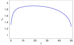
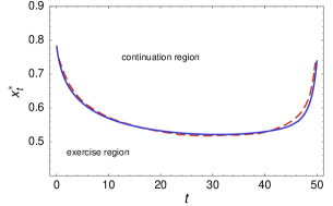
Refer to caption
Refer to caption
Figure 2: The function ϱ(τ)italic-ϱ𝜏\varrho(\tau) (left). A comparison of the free boundary position xt=1/ϱ(Tt)subscriptsuperscript𝑥𝑡1italic-ϱ𝑇𝑡x^{*}_{t}=1/\varrho(T-t) (right) obtained by our method (solid curve) and that of the projected successive over relaxation algorithm by Dai and Kwok (dashed curve).
Refer to caption
Refer to caption
Refer to caption
Figure 3: A 3D plot (left) and contour plot (right) of the function Π(ξ,τ)Π𝜉𝜏\Pi(\xi,\tau). Profiles of the function Π(ξ,τ)Π𝜉𝜏\Pi(\xi,\tau) for various times τ[0,T]𝜏0𝑇\tau\in[0,T].

In Fig. 3 we can see the behavior of the transformed function ΠΠ\Pi in both 3D as well as contour plot perspectives. We also plot the initial condition Π(ξ,0)Π𝜉0\Pi(\xi,0) and five time steps of the function ξΠ(ξ,τj)maps-to𝜉Π𝜉subscript𝜏𝑗\xi\mapsto\Pi(\xi,\tau_{j}) for τj=0.1,1,5,25,50subscript𝜏𝑗0.1152550\tau_{j}=0.1,1,5,25,50.

A comparison of early exercise boundary profiles with respect to varying interest rates r𝑟r and dividend yields q𝑞q is shown in Fig. 4. A comparison of the free boundary position xt=1/ϱ(Tt)subscriptsuperscript𝑥𝑡1italic-ϱ𝑇𝑡x^{*}_{t}=1/\varrho(T-t) obtained by our method (solid curve) and that of the projected successive over relaxation algorithm by (?) (dashed curve) for different values of the interest rate r𝑟r is shown in Fig. 4 (right). The algorithm of (?) is based on a numerical solution to the variational inequality for the function W=W(x,τ)𝑊𝑊𝑥𝜏W=W(x,\tau) which a solution to (21) in the continuation region and it is smoothly pasted to its pay-off diagram (23). It is clear that our method and that of (?) give almost the same results. A quantitative comparison of both methods is given in Table 4 for model parameters T=50,σ=0.2,q=0.04formulae-sequence𝑇50formulae-sequence𝜎0.2𝑞0.04T=50,\sigma=0.2,q=0.04 and various interest rates r=0.02,0.04,0.06𝑟0.020.040.06r=0.02,0.04,0.06. We evaluated discrete L(0,T)superscript𝐿0𝑇L^{\infty}(0,T) and L1(0,T)superscript𝐿10𝑇L^{1}(0,T) norms of the difference xt,transxt,psorsubscriptsuperscript𝑥𝑡𝑟𝑎𝑛𝑠𝑡subscriptsuperscript𝑥𝑝𝑠𝑜𝑟𝑡x^{*,trans}_{t}-x^{*,psor}_{t} between the numerical solution xt,trans,t[0,T],subscriptsuperscript𝑥𝑡𝑟𝑎𝑛𝑠𝑡𝑡0𝑇x^{*,trans}_{t},t\in[0,T], obtained by our method and that of (?) denoted by xt,psorsubscriptsuperscript𝑥𝑝𝑠𝑜𝑟𝑡x^{*,psor}_{t}. We also show the minimal value mint[0,T]xt,transsubscript𝑡0𝑇subscriptsuperscript𝑥𝑡𝑟𝑎𝑛𝑠𝑡\min_{t\in[0,T]}x^{*,trans}_{t} of the early exercise boundary.

Table 4: Comparison of PSOR and our transformation method for T=50,σ=0.2,q=0.04formulae-sequence𝑇50formulae-sequence𝜎0.2𝑞0.04T=50,\sigma=0.2,q=0.04.
r=0.06𝑟0.06r=0.06 r=0.04𝑟0.04r=0.04 r=0.02𝑟0.02r=0.02
xt,transxt,psorsubscriptnormsubscriptsuperscript𝑥𝑡𝑟𝑎𝑛𝑠𝑡subscriptsuperscript𝑥𝑝𝑠𝑜𝑟𝑡\|x^{*,trans}_{t}-x^{*,psor}_{t}\|_{\infty} 0.09769 0.03535 0.05359
xt,transxt,psor1subscriptnormsubscriptsuperscript𝑥𝑡𝑟𝑎𝑛𝑠𝑡subscriptsuperscript𝑥𝑝𝑠𝑜𝑟𝑡1\|x^{*,trans}_{t}-x^{*,psor}_{t}\|_{1} 0.00503 0.00745 0.01437
minxt,transsubscriptsuperscript𝑥𝑡𝑟𝑎𝑛𝑠𝑡\min x^{*,trans}_{t} 0.52150 0.57780 0.63619

Finally, in Fig. 5 we present numerical experiments for shorter expiration times T=0.7𝑇0.7T=0.7 and T=1𝑇1T=1 (one year) with zero dividend rate q=0𝑞0q=0 and r=0.06,σ=0.2formulae-sequence𝑟0.06𝜎0.2r=0.06,\sigma=0.2. We also present a comparison of the free boundary position xt=1/ϱ(Tt)subscriptsuperscript𝑥𝑡1italic-ϱ𝑇𝑡x^{*}_{t}=1/\varrho(T-t) and the analytic approximation (17) for parameters: r=0.06,q=0,σ=0.2formulae-sequence𝑟0.06formulae-sequence𝑞0𝜎0.2r=0.06,q=0,\sigma=0.2 and T=1𝑇1T=1. It is clear that the analytic approximation (17) is capable of capturing the behavior of xtsubscriptsuperscript𝑥𝑡x^{*}_{t} only for times t𝑡t close to the expiry T𝑇T. Moreover, the analytic approximation is a monotone function whereas the true early exercise boundary xtsubscriptsuperscript𝑥𝑡x^{*}_{t} is a decreasing function for small values of t𝑡t and then it becomes increasing (see e.g. Fig. 5).
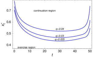
Refer to caption
Refer to caption
Figure 4: A comparison of the free boundary position xtsubscriptsuperscript𝑥𝑡x^{*}_{t} for various dividend yield rates q=0.04,0.03,0.025𝑞0.040.030.025q=0.04,0.03,0.025 and fixed interest rate r=0.06𝑟0.06r=0.06 (left). Comparison of xtsubscriptsuperscript𝑥𝑡x^{*}_{t} for various interest rates r=0.06,0.04,0.02𝑟0.060.040.02r=0.06,0.04,0.02 and fixed dividend yield q=0.04𝑞0.04q=0.04. Dots represents the solution obtained by Dai and Kwok (right).
Refer to caption
Refer to caption
Refer to caption
Figure 5: The free boundary position for expiration times T=0.7𝑇0.7T=0.7 (left) and T=1𝑇1T=1 (center). A comparison of the free boundary position with its the analytic approximation (dashed line).

Conclusions

In this paper we analyzed American-style Asian options with averaged floating strike. We focused on arithmetic, geometric and weighted arithmetic averaging of the floating strike price. In the first part of the paper we derived an integral representation of the call and put option prices and we provided an integral equation for the free boundary position. We analyzed the behavior of the early exercise boundary close to expiry. We proposed a general methodology how to determine the early exercise position at expiry. We furthermore derived the asymptotic formula for the early exercise boundary close to the expiry. The second part of the paper was devoted to construction of a robust numerical scheme for finding an approximation of the early exercise boundary. Applying the front fixing method, we derived a nonlocal parabolic partial differential for the synthetised portfolio and the free boundary position. Using an idea of the operator splitting technique we moreover constructed a numerical scheme for numerical solution of the problem. The capability of the method has been documented by several computational examples.

Acknowledgments

This research was supported by VEGA 1/0381/09 and APVV SK-BG-0034-08 grants.

References

  • [1]
  • [2] [] Chadam, J.: 2008, Free boundary problems in mathematical finance, Progress in industrial mathematics at ECMI 2006, Vol. 12 of Math. Ind., Springer, Berlin, pp. 655–665.
  • [3]
  • [4] [] Dai, M. and Kwok, Y. K.: 2006, Characterization of optimal stopping regions of American Asian and lookback options, Math. Finance 16(1), 63–82.
  • [5]
  • [6] [] Detemple, J.: 2006, American-Style Derivatives: Valuation and Computation, Chapman and Hall/CRC.
  • [7]
  • [8] [] Dewynne, J. N., Howison, S. D., Rupf, I. and Wilmott, P.: 1993, Some mathematical results in the pricing of American options, European J. Appl. Math. 4(4), 381–398.
  • [9]
  • [10] [] Geske, R. and Johnson, H. E.: 1984, The American put option valued analytically, J. Finance 39, 1511–1524.
  • [11]
  • [12] [] Geske, R. and Roll, R.: 1984, On valuing American call options with the Black–Scholes European formula, J. Finance 89, 443–455.
  • [13]
  • [14] [] Hansen, A. T. and Jørgensen, P. L.: 2000, Analytical valuation of American-style Asian options, Management Science 46(8), 1116–1136.
  • [15]
  • [16] [] Hull, J. C.: 1997, Options, Futures and Other Derivative Securities, third edn, Prentice Hall.
  • [17]
  • [18] [] Karatzas, I.: 1988, On the pricing American options, Appl. Math. Optim. 17, 37–60.
  • [19]
  • [20] [] Kim, B. C. and Oh, S. Y.: 2004, Pricing of American-style fixed strike Asian options with continuous arithmetic average.
  • [21]
  • [22] [] Kuske, R. A. and Keller, J. B.: 1998, Optimal exercise boundary for an American put option, Applied Mathematical Finance 5, 107–116.
  • [23]
  • [24] [] Kwok, Y. K.: 1998, Mathematical models of financial derivatives, Springer Finance, Springer-Verlag Singapore, Singapore.
  • [25]
  • [26] [] Kwok, Y. K.: 2008, Mathematical models of financial derivatives, Springer Finance, second edn, Springer, Berlin.
  • [27]
  • [28] [] Linetsky, V.: 2004, Spectral expansions for Asian (average price) options, Operations Research 52(6), 856–867.
  • [29]
  • [30] [] Mallier, R.: 2002, Evaluating approximations for the American put option, Journal of Applied Mathematics 2, 71–92.
  • [31]
  • [32] [] Pascucci, A.: 2008, Free boundary and optimal stopping problems for American Asian options, Finance Stoch 12, 21–41.
  • [33]
  • [34] [] Revuz, D. and Yor, M.: 2005, Continuous martingales and Brownian motion, Vol. 293 of Grundlehren der Mathematischen Wissenschaften [A Series of Comprehensive Studies in Mathematics], corrected third edn, Springer-Verlag, Berlin.
  • [35]
  • [36] [] Ševčovič, D.: 2001, Analysis of the free boundary for the pricing of an American call option, European J. Appl. Math. 12(1), 25–37.
  • [37]
  • [38] [] Ševčovič, D.: 2007, An iterative algorithm for evaluating approximations to the optimal exercise boundary for a nonlinear Black-Scholes equation, Canad. Appl. Math. Quart. 15(1), 77–97.
  • [39]
  • [40] [] Ševčovič, D.: 2009, Transformation methods for evaluating approximations to the optimal exercise boundary for a linear and nonlinear Black-Scholes equation, in M. Ehrhardt (ed.), Nonlinear Models in Mathematical Finance: New Research Trends in Option Pricing, Nova Science Publishers, New York, pp. 153–198.
  • [41]
  • [42] [] Stamicar, R., Ševčovič, D. and Chadam, J.: 1999, The early exercise boundary for the American put near expiry: numerical approximation, Canad. Appl. Math. Quart. 7(4), 427–444.
  • [43]
  • [44] [] Wilmott, P., Howison, S. and Dewynne, J.: 1995, The mathematics of financial derivatives, Cambridge University Press, Cambridge. A student introduction.
  • [45]
  • [46] [] Wu, L., Kwok, Y. K. and Yu, H.: 1999, Asian options with the American early exercise feature, International Journal of Theoretical and Applied Finance 2(1), 101–111.
  • [47]
  • [48] [] Wu, R. and Fu, M. C.: 2003, Optimal exercise policies and simulation-based valuation for American-Asian options, Operations Research 51(1), 52–66.
  • [49]
  • [50] [] Wystup, U.: 2006, FX Options and Structured Products, www.mathfinance.com.
  • [51]