Automatic creation of urban velocity fields from aerial video

Abstract

In this paper, we present a system for modelling vehicle motion in an urban scene from low frame-rate aerial video. In particular, the scene is modelled as a probability distribution over velocities at every pixel in the image.

We describe the complete system for acquiring this model. The video is captured from a helicopter and stabilized by warping the images to match an orthorectified image of the area. A pixel classifier is applied to the stabilized images, and the response is segmented to determine car locations and orientations. The results are fed in to a tracking scheme which tracks cars for three frames, creating tracklets. This allows the tracker to use a combination of velocity, direction, appearance, and acceleration cues to keep only tracks likely to be correct. Each tracklet provides a measurement of the car velocity at every point along the tracklet’s length, and these are then aggregated to create a histogram of vehicle velocities at every pixel in the image.

The results demonstrate that the velocity probability distribution prior can be used to infer a variety of information about road lane directions, speed limits, vehicle speeds and common trajectories, and traffic bottlenecks, as well as providing a means of describing environmental knowledge about traffic rules that can be used in tracking.

I Introduction

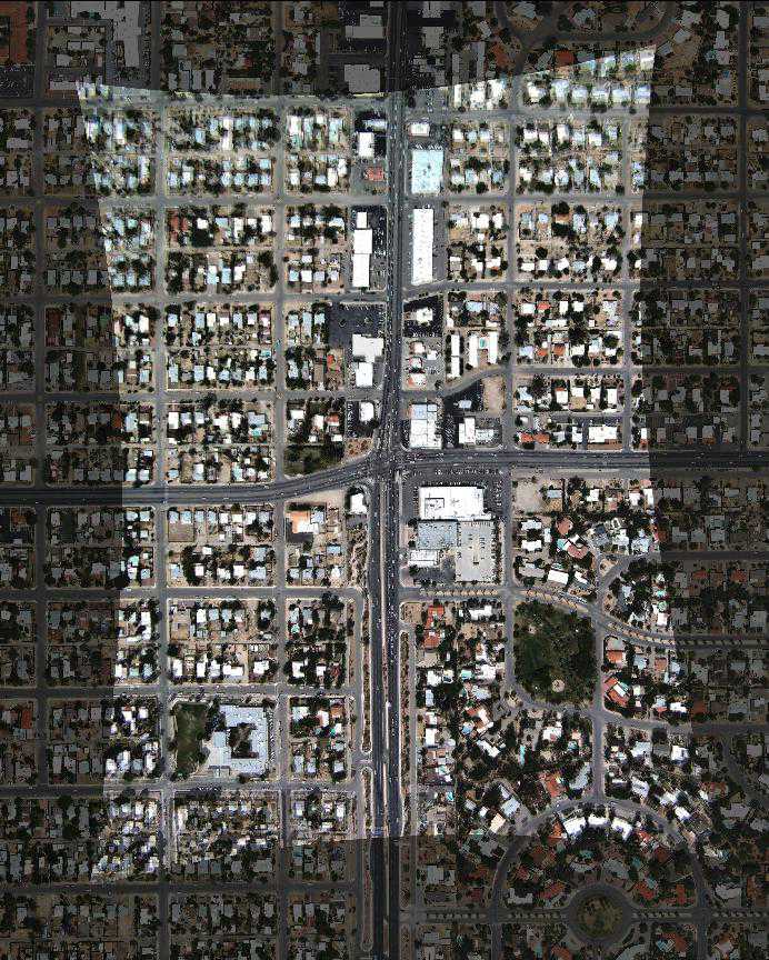
The increasingly widespread availability of high-resolution video sensors, coupled with improvements in accompanying storage media, and processors have made the collection of aerial video for the purposes of tracking automobiles and monitoring traffic much more feasible in recent years [1]. Corresponding efforts for the acquisition of aerial video imagery of traffic data using helicopters for the flight platform have been conducted by Angel et al. [2], Ernst et al. [3], Ruhé et al. [4], Hoogendoorn [5] and Hoogendoorn and Schreuder [6]. More recently, a data collect has been conducted in a joint effort between Los Alamos National Laboratory (LANL) and the University of Arizona, a frame of which is shown in Figure 1.

Figure 1: A video frame taken from the helicopter superimposed over an image of the same region acquired from ‘Google™  Maps’. The curved boundaries of the image are due to the radial distortion correction and registration processes.

Aerial video is useful for traffic monitoring, since a large amount of data can be collected without the need to manually instrument large areas with sensors. Therefore, it is often desirable when collecting such video data to maximize the area covered. Limitations on storage, communications bandwidth and sensor resolution result in trade-offs between the area and other system parameters. In those cases where maximum area coverage is a strong driver, the number of pixels on target and the sampling rate will both tend to be low. This in turn tends to reduce tracking performance, in that virtually all tracking algorithms are based on: 1) appearance cues, which require enough pixels on target so that neighboring targets are distinguishable, and/or 2) smooth trajectory assumptions, which are broken if sampling rates fall too low with respect to the underlying spatial frequencies of the target trajectories.

In certain situations, tracking can be used to deduce rules underlying the system being tracked (such as, for example occlusions [7]). In urban environments in particular, such rules are reflected by the existence of restricted regions (i.e. cars don’t drive through walls), as well as high probabilities of certain speeds and directions of travel in allowed regions (i.e. traffic lanes have directions and speed limits). With this dataset, however we do not need to implement a complete, fully automated tracking system to get these results. Instead, we use a scheme whereby we find short tracks which are likely to be correct by ignoring difficult situations such as ambiguity, failure to detect cars, or false positives. Since we have a large amount of data, we can aggregate all data from all the short tracks over many frames to generate a model representing the rules.

In this paper, we outline an algorithm that effectively allows the inference of these rules by building up a velocity histogram at each pixel in the scene, continuing our previous work in [8]. In Section II, we describe the system for acquiring and processing data suitable for the analysis we are performing in this paper. This analysis is done using track fragments, and takes advantage of the extremely high amount of information available to allow the application of a car detector (Section III) followed by a tracking/data association algorithm (Section IV) which only retains tracks which are likely to be correct. These tracks are then used to build a model of the city (Section V), represented as a velocity probability distributions at each pixel. We then present the results in Section VI and discuss how this provides advantages not only for future tracking algorithms, but also insight into the transportation structure of the urban environment.

II Data collection and initial processing

The data was collected in a six passenger Bell JetRanger helicopter, hovering above Tucson, Arizona (nominally at 32.250^∘ N, 110.944^∘ W), with one door off to allow for cables to be passed through. The sensor used was an InVision IQEye 705 camera with the vendor’s V10 optics package. The sensor was rigidly mounted to the helicopter strut, with an ethernet interface to a laptop for data storage and power transmission. A marine battery was carried along in the back seat as a power source. Details of the imaging parameters are given in Table I.

Parameter	Value
Image Size	$2560\times 1920$ pixels
Sampling Rate	$\sim 5$ frames/second$\dagger$
Spatial Resolution	$\sim 23$ cm/pixel at the centre
Helicopter Altitude	$\sim 900$ m (above ground level)
Field of view	$\sim 70^{\circ}$

TABLE I: Data capture parameters. $\dagger$Note that the fame rate was not entirely constant. The camera would occasionally delay frame capture by a half or full frame interval.

Figure 2: Two frames from the aerial video dataset, taken 20s apart.. Note the large amount of radial distortion and motion between these frames.

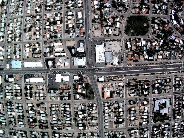
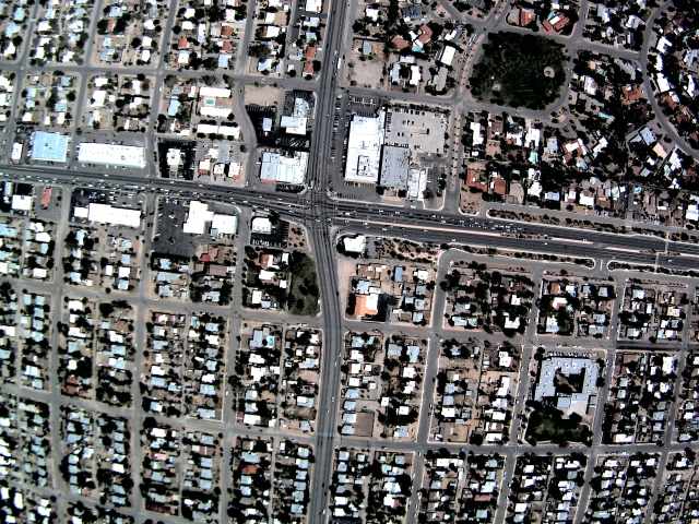
An example of two frames of data are shown in Figure 2. Several features of the data can be seen from this, namely that the camera has a large amount of radial distortion, and that the images require stabilization. Distortions not readily apparent from this image are due to the ground being non-planar, and the rolling shutter on the camera. The rolling shutter is caused by pixels being exposed shortly before the row is clocked out of the CCD, so rows towards the bottom of the image are exposed later than rows at the top. This interacts with the high frequency vibration of the helicopter and results in image distortion with a high spatial frequency. This necessitates the use of a model with a large number of parameters, so we used a robust coarse-to-fine strategy.

For a general treatment of image registration, see for example [9, 10]. In our case, registration was performed in several stages. Firstly, the parameters of the radial distortion were found using the method in [11], which uses the ‘plumb-line constraint’ (the assumption of the existence of long, straight lines) to determine the distortion parameters. These parameters were then used to undistort all of the images.

Then, a single image was orthorectified by registering it to an aerial image taken from Google Maps (intersensor registration). An initial, coarse registration was performed by matching SIFT [12] features between $\frac{1}{4}$ sized versions of the two images, and fitting a homography using RANSAC [13] for robust estimation. Due to the difficulties of matching feature points between images taken with different sensors, this is able to fit the homography to within about a 20% error in scale and about 10^∘ in rotation.

A second stage of matching was then performed using a square grid of predetermined points, with a 50 pixel spacing between points, giving about 2000 points in total. A $75\times 75$ patch of pixels was taken around each grid point in the helicopter image. These patches were then matched to a region around the corresponding grid point in the Google Maps image, using normalized cross correlation. A second order polyprojective model (also known as a rational function model [14] or nonlinear homography [15]) was then fitted to these using a robust technique. In particular, we used a case deletion scheme where the model is fitted to the matches by minizing the sum-squared error using the Downhill-Simplex [16] algorithm. The worst 5% of points are removed and the model is refitted. The procedure is iterated until the mean error drops below 2 pixels.

The result of this is a single orthorectified helicopter image, which we refer to as the ‘base image’. Subsequent images in the video are then registered to the base image, which is intrasensor registration. The intrasensor registration process is inherently more forgiving than the intersensor process. This in turn allows the usage of different subalgorithms which provide much denser coverage of the image with better matching accuracy. The registration processes are still similar, however, in that a coarse to fine approach is still used, as is the basic framework of finding an optimal set of transform parameters from an iteratively refined set of control point matches. Frames of the video are registered simultaneously to the base image and the previous registered image. This removes long term drift and alleviates the problem that the area of overlap with the base image may be small.

The first stage of the intersensor registration matches SIFT keypoints between the current and previous/base image. An approximate transformation for the current image is known, since we know the transformation for the previous image. Therefore, the SIFT keypoints in the current image are only allowed to match to points within a $50\times 50$ pixel region in the previous/base image. A polyprojective transformation is then fitted using the case deletion scheme.

After this stage, errors with high spatial frequency remain as a result of the rolling shutter. To fit these errors, the image is split up in to $200\times 200$ cells, and a displacement vector is robustly found for each cell. Intermediate displacements are found by linearly interpolating the vectors between the cell centres. The vectors are found by matching the SIFT keypoints between a cell in the current image and the corresponding cell in the previous/base image. Case deletion is then used to find the best single displacement vector for each cell.

These stages of registration bring the average jitter down to about 1 pixel, and the registered images are used for the remainder of the paper. For the interested reader, a more detailed treatment of these steps is also given in [17].

III Car detection

A number of existing vehicle-specific techniques assume that either a single car orientation, or a small subset of possible orientations, is known [18, 19]. These techniques are unsuitable for our application, since cars can appear at any orientation, for instance turning a corner at a junction. Other algorithms [20, 21, 22] use road position information from maps to aid detection. These techniques will therefore ignore traffic in parking lots and are not applicable where the road information is not up to date, such as during major engineering works or evacuation situations. Traffic monitoring would be particularly useful in these situations. Other techniques [23] are designed for accurate car counting, and so are tuned to perform well in parking lots, where large number of parallel cars are parked close together. Model based techniques, such as [24] tend to work with approximately 2 to 3 times the ground sample distance of our data. Consequently, we decided to use an approach based on generic object detection.

Car detection is performed by following the steps:

1. Apply pixel classifier to image and record the classifier response at each pixel in to a ‘response image’.

2. Blur the response image with a Gaussian.

3. Find all local maxima of the blurred response image.

4. Perform region growing segmentation of the response image, starting from the maxima.

5. Filter out small regions.

6. Compute mean and covariance of pixel positions in remaining regions.

7. A car is located at the mean of each region, oriented along the direction of largest covariance.

Pixel classification is performed in a similar manner to the method presented in [25], though somewhat simplified since processing speed is not a concern. The centres of all cars in an image were marked. Any pixel within 6 pixels distance of a car centre was labelled as a foreground pixel. Any pixel not within 20 pixels of any car center was labelled as a background pixel. Pixels an intermediate distance from cars are unmarked. In our dataset, cars are approximately 8 pixels wide and 16 pixels in length. The background pixels are then randomly subsampled so that foreground pixels make up about 15% of the data (as opposed to 1%). A single image was marked, giving 330 cars and 300,000 labelled pixels. We then trained an AdaBoost [26] classifier on the data for 200 iterations.

Weak classifiers are similar to the features in [25, 27], in that we use a sum of positive and negative rectangles. In our case, we have between 1 and 5 rectangles of each sort, and the corners of the rectangles are scatted at random with a Gaussian distribution with $\sigma=10$ pixels. This allows the rectangles to overlap.

To detect cars, the classifier is then applied to the image. For typical applications of machine learning, the response of the classifier would be thresholded at zero, giving the class of each pixel. However, we wish to find cars, rather than the class of each pixel. To do this, the classifier response is smoothed with a Gaussian kernel (with $\sigma=3$ pixels), and all the local maxima are found and taken as candidate car locations.

Region growing segmentation is performed iteratively from these candidate locations until no further changes happen. The image corresponding to the blurred response of the classifier is denoted $C$ and the segmented image at iteration $t$ is denoted $S_{t}$. The segmentation $S_{0}$ is initialized such that each pixel under a local maximum of $C$ is given a unique number, and every other pixel has the value 0.

The iteration sequence generates $S_{t}$ from $S_{t-1}$. Initially, we assign $S_{t}\leftarrow S_{t-1}$. For each occupied pixel $(x,y)$ in $S_{t-1}$, i.e. where $S_{t-1}(x,y)\neq 0$, we attempt to spread the pixel value to its neighbours. Consider the pixel $(x,y)$ which we attempt to spread to its neighbour, $(x+\delta_{x},y+\delta_{y})$. If $S_{t}(x+\delta_{x},y+\delta_{y})=0$ (the neighbouring pixel is unoccupied) and if $C(x+\delta_{x},y+\delta_{y})>T$ (the response is above some threshold), then assign $S_{t}(x+\delta_{x},y+\delta_{y})\leftarrow S_{t-1}(x,y)$. We use 4-neighbour connectivity, $(\delta_{x},\delta_{y})$ takes the values $(1,0),(-1,0),(0,1)$ and $(0,-1)$. This procedure is iterated until $S_{t}=S_{t+1}$.

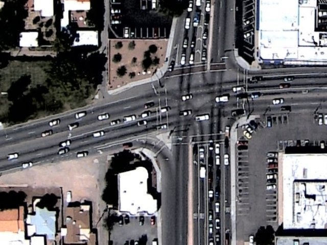
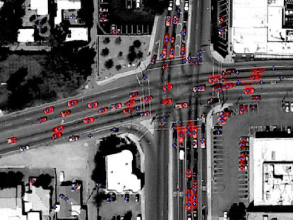
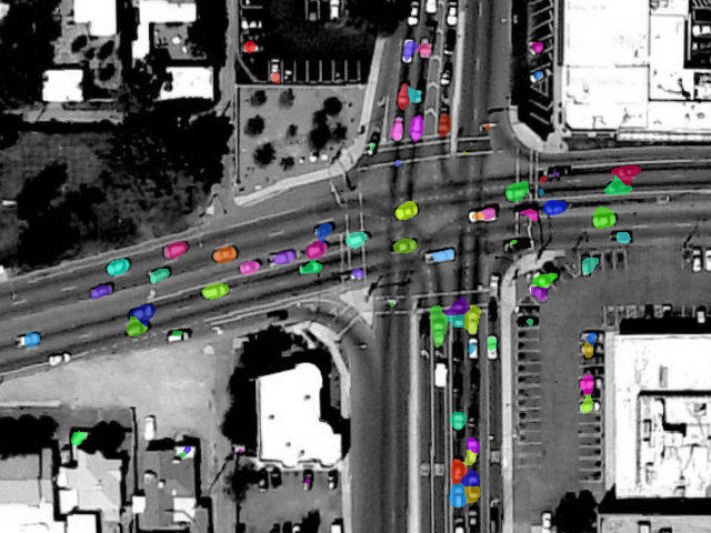
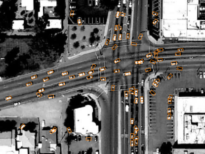
At this point, all pixels sharing the same, nonzero number belong to the same object. Small objects are filtered out by removing objects that do not have enough pixels. In this case, segments with fewer than 10 pixels are removed. Of the remaining objects, their position and orientation are found by computing the mean and covariance of the pixels. It is assumed that cars are aligned along the direction of largest covariance. This does not distinguish between the front and back of cars. An illustration of this process is given in Figure 3.

1	2
3	4

Figure 3: 1. Original image. Note that processing is performed in greyscale. 2. Blurred classifier response ($C$). The classifier response (where positive) is shown superimposed in red on the original image. Candidate car locations are shown at the local maxima, marked by blue ‘+’ marks. 3. Result of grown regions ($S_{\infty}$). A colour was selected at random for each region. 4. The detected cars superimposed on the original image. The rectangle representing detected cars are drawn at a predetermined size.

IV Tracking

There are a number of approaches to tracking multiple targets in the presence of detection errors and measurement noise, such as JPDAF (Joint Probabilistic Data Association Filter) [28], SMC (Sequential Monte-Carlo) [29] and PHD (Probability Hypothesis Density) filter [30], which can integrate continuity assumptions such as smoothness of motion and continuity of appearance. The main focus of these methods is to produce long tracks which are as accurate as possible, and get the correct data association over a large number of measurements.

Since we wish to build up a model of car motion over the city, we can aggregate a large amount of data from many frames. As a result, the tracking algorithm does not need to reliably produce long, accurate tracks. Instead we focus on forming short, but correct track fragments. Data which makes tracking more difficult, such as false negatives, false positives, and misestimation of the car orientation simply causes the track to be discarded.

Without any knowledge of the system, a car in frame $n$ could match to any of the cars in frame $n+1$. The algorithm relies on basic physics to eliminate the majority of potential matches. A car in frame $n$ can only match to a car located within 30 pixels of it in frame $n+1$. Given the frame rate and pixel size, this corresponds to a maximum velocity of 78 mph (124 km/h). Similarly, matches where a car rotates more than 30^∘ between frames are eliminated. Furthermore, matches where the direction of motion is more than 30^∘ off the direction of the car are eliminated. This last constraint is not applied if the velocity is below 5 pixels/s since noise from misregistration jitter prevents accurate measurement of the direction of motion.

When a car in frame $n$ can still potentially match to more than one car in frame $n+1$, we use appearance based symmetric matching [31]. That is, for each car in frame $n$, we pick the best match in frame $n+1$, and for every car in frame $n+1$, we pick the best match in frame $n$. Only the matches which are consistent are retained. The quality of a match is measured by using the sum of absolute differences (SAD) of a $8\times 16$ pixel rectangular patch, centred on a car and aligned with its direction. The best match is the one with the smallest SAD.

The same process is then repeated between frames $n+1$ and $n+2$, and the resulting matches are chained together to create 3 frame ‘tracklets’. Tracklets with an unphysically high acceleration are removed. Although 1g corresponds to 1.74 pixels/frame/frame, we allow for an acceleration of up to 4 pixels/frame/frame to take into account jitter caused by misregistration.

V Model building

Once the tracklets have been found over all frames, they are used to build a model of the vehicle motion in the image. The model for motion is built up at every pixel and contains a 2D histogram of motion vectors. The tracklets consist of two line segments, and the two line segments each have an associated velocity vector. A line segment is placed in to the model by incrementing histogram bins corresponding to the velocity at every position along the line segments. All line segments from all tracklets are used to create the model. For increased precision and smoothness, instead of simply incrementing the closest bin to the velocity vector, a smooth Gaussian blob centred on the velocity vector is entered in to the histogram.

VI Results and Discussion

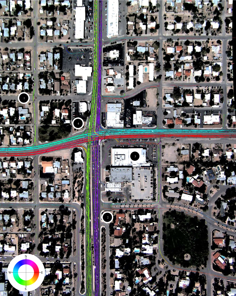
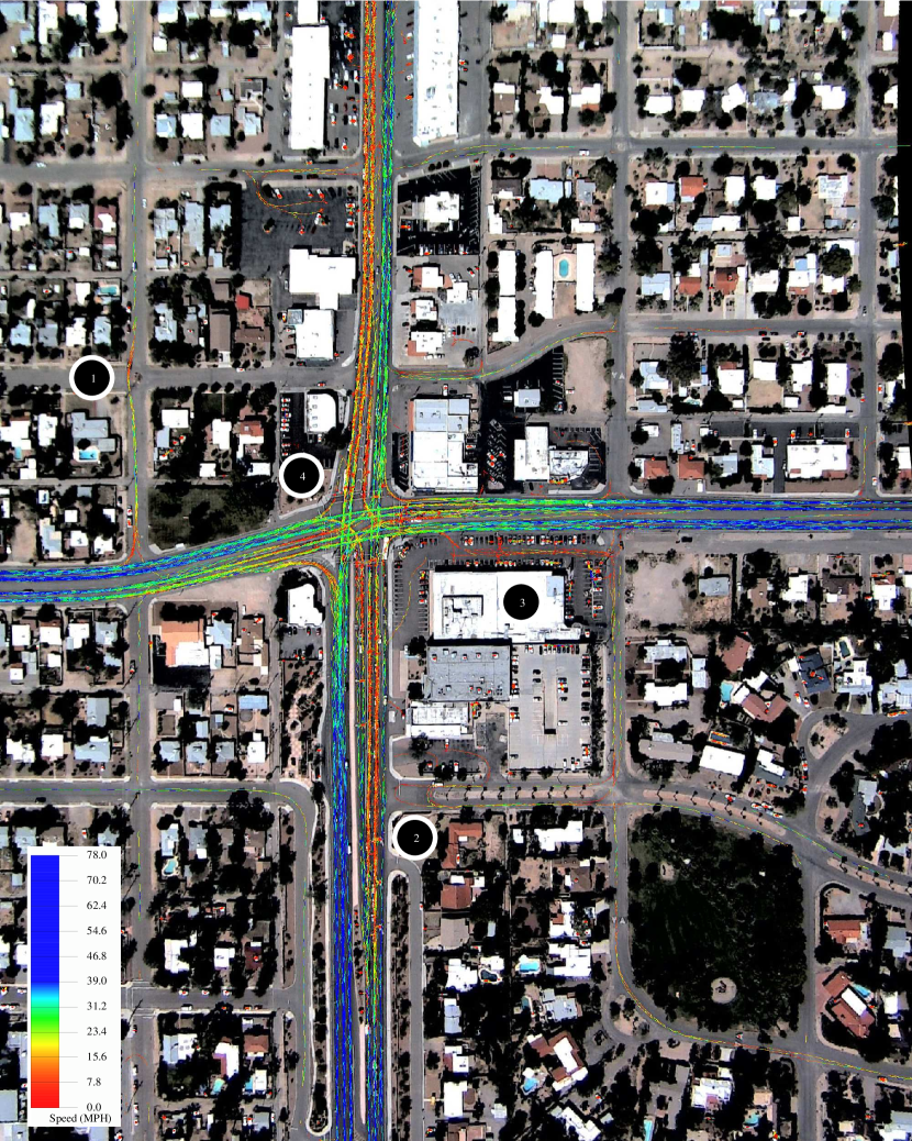
The modes of the histograms at each pixel built from a dataset are shown in Figures 4 and 5. Examination of this data directly provides a large amount of information useful for traffic engineering and planning. Such data would be very expensive to obtain using standard techniques. Existing loop detectors or pneumatic tubes cannot capture vehicle trajectories; fixed cameras often do not have an extended field of view or suffer from occlusion; and, floating car techniques are expensive and provide only very small samples of vehicles.

Some interesting parts to note (labelled in Figures 4 and 5) are:

1. The traffic circle at this unsignalized intersection is effective and causes a significant reduction in the speed of the vehicle. However, despite the presence of the junction close to the south, drivers consistently accelerate rapidly up to the nominal speed for this road.

2. A large number of U-turns at this particular junction imply that vehicles are unwilling to enter the main northbound traffic stream at this location. There may be significant delay for vehicles at this junction, and/or there may be inadequate signage to deter U-turns. Note that there is a central median on the major street which prevents traffic from turning into a southbound lane at this point.

3. This parking lot exhibits significant traffic in the easterly direction, with cars entering on the west and driving through to the east exit. With the proximity to the major intersection (seen at the center of the image), it may be beneficial to prevent cars exiting in the north-west corner, to prevent congestion and possible conflicts at this intersection.

   A failure mode of the algorithm can be seen due east of the label. The car detector tends to misdetect cars and misestimate the orientation in parking lots, especially when the cars are densely packed. This occasionally causes mismatches, and therefore erroneous tracklets, the results of which can be seen.

4. The modal speed through the junction is lower than the nominal road speed. This implies that even on a green light, there may be factors that are causing drivers to slow, and reducing the flow of traffic. Also, the traffic speeds are significantly lower in the north-south direction, with significant queuing and very low speeds indicated by the tracklets. This would clearly imply that the allocation of green time at this traffic signal may need to be adjusted to give more green time to north-south movements.

   The tracklets exiting the major intersection to the south indicate some significant lane changing activity. This may occur in part due to potential conflicts from the right-turning traffic from the eastbound approach to the southbound exit. This activity may also be due in part from the expansion of the roadway from two to three lanes as traffic moves southbound from the intersection. It may be useful to delineate the appropriate paths of vehicles more clearly through this section of roadway.

   Similar lane changing can be noted on the eastbound exit of this intersection, but the causes of these lane changes is not readily apparent.

Figure 4: Direction of the mode of the histograms at each pixel, for a cutout of the image. Where no information has been added to a histogram, the original image is shown. The complete images have been included in the supplementary material. Note that where the modal speed is zero, no direction has been drawn in. The model was computed from 1126 frames (about 4 minutes of data). Interesting parts of the data (in both images) have been labelled in the upper image, and the complete images have been included in the supplementary material.

Figure 5: Speed of the mode of the histograms at each pixel, for a cutout of the image. Where no information has been added to a histogram, the original image is shown. The complete images have been included in the supplementary material. Note that where the modal speed is zero, no direction has been drawn in. The model was computed from 1126 frames (about 4 minutes of data). Interesting parts of the data (in both images) have been labelled in the upper image, and the complete images have been included in the supplementary material.

References

- [1] R. Kumar, H. Sawhney, S. Samarasekera, S. Hsu, H. Tao, Y. Guo, K. Hanna, A. Pope, R. Wildes, D. Hirvonen, M. Hansen, and P. Burt, “Aerial video surveillance and exploitation,” Proceedings of the IEEE, vol. 89, no. 10, pp. 1518–1539, Oct. 2001. [Online]. Available: http://ieeexplore.ieee.org/iel5/5/20732/00959344.pdf
- [2] A. Angel, M. Hickman, P. Mirchandani, and D. Chandnani, “Methods of analyzing traffic imagery collected from aerial platforms,” IEEE Transactions on Intelligent Transportation Systems, vol. 4, no. 2, pp. 99–107, Jun. 2003.
- [3] S. Ernst, S. Zuev, K. Thiessenhausen, M. Hetscher, S. Rassmann, and M. Ruhè, “Lumos - airborne traffic monitoring system,” in Proceedings of the IEEE 6th International Conference on Intelligent Transportation Systems, Shanghai, China, 2003.
- [4] M. Ruh , R. K hne, I. Ernst, S. Zuev, and E. Hipp, “Airborne systems and data fusion for traffic surveillance and forecast for the soccer world cup,” in Paper presented at the 2007 Annual Meeting. Transportation Research Board, 2007.
- [5] S. Hoogendoorn, H. Van Zuylen, M. Schreuder, B. Gorte, and G. Vosselman, “Microscopic traffic data collection by remote sensing,” Transportation Research Record, vol. 1855, pp. 121–128, 2003. [Online]. Available: http://www.itc.nl/personal/vosselman/papers/hoogendoorn2003.trb.pdf
- [6] S. Hoogendoorn and M. Schreuder, “Tracing congestion dynamics with remote sensing,” in Paper presented at the 2007 Annual Meeting. Transportation Research Board, 2005.
- [7] D. Greenhill, J. Rennoa, J. Orwella, and G. Jones, “Occlusion analysis: Learning and utilising depth maps in object tracking,” Image and Vision Computing, vol. 26, no. 3, pp. 430–441, Mar. 2008.
- [8] R. C. Loveland, E. Rosten, and R. Porter, “Improving multiple target tracking in structured environments using velocity priors,” in Proceedings of the SPIE: Signal and Data Processing of Small Targets 2008, April 2008, pp. 69 690H–69 690H–8.
- [9] L. G. Brown, “A survey of image registration techniques,” ACM Computing Survey, vol. 24, no. 4, pp. 325–376, 1992.
- [10] B. Zitova and J. Flusser, “Image registration methods: a survey,” Image and Vision Computing, vol. 21, no. 11, pp. 977–1000, Oct. 2003.
- [11] E. Rosten and R. Loveland, “Camera distortion self-calibration using the plumb-line constraint and minimal hough entropy,” Machine Vision and Applications, October 2009. [Online]. Available: http://lanl.arXiv.org/pdf/0810.4426
- [12] D. G. Lowe, “Distinctive image features from scale-invariant keypoints,” International Journal of Computer Vision, vol. 60, no. 2, pp. 91–110, Nov. 2004.
- [13] M. A. Fischler and R. C. Bolles, “Random sample consensus: A paradigm for model fitting with applications to image analysis and automated cartography,” Communcations of the ACM, vol. 24, no. 6, pp. 381–395, Jun. 1981.
- [14] D. Claus and A. Fitzgibbon, “A rational function lens distortion model for general cameras,” IEEE Computer Society Conference on Computer Vision and Pattern Recognition, vol. 1, pp. 213–219, 2005.
- [15] E. Rosten and S. Cox, “Accurate extraction of reciprocal space information from transmission electron microscopy images,” in Advances in Visual Computing. LNCS 4292, vol. 1, November 2006, pp. 373–382. [Online]. Available: http://mi.eng.cam.ac.uk/~er258/work/rosten_2006_accurate.pdf
- [16] J. Nelder and R. Mead, Computer Journal, vol. 7, pp. 308–313, 1965.
- [17] R. C. Loveland and E. Rosten, “Acquisition and registration of aerial video imagery of urban traffic,” in Applications of Digital Image Processing XXXI, vol. 7030, October 2008, pp. 70 731N–70 731N–12. [Online]. Available: http://mi.eng.cam.ac.uk/~er258/work/loveland_2008_acquisition.pdf
- [18] T. Zhao and R. Nevatia, “Car detection in low resolution aerial images,” Image and Vision Computing, vol. 21, no. 8, pp. 693–703, Aug. 2003. [Online]. Available: http://iris.usc.edu/Outlines/papers/2003/IVC03-zhao-car.pdf
- [19] Z. W. Kim and J. Malik, “Fast vehicle detection with probabilistic feature grouping and its application to vehicle tracking,” in 9 IEEE International Conference on Computer Vision, vol. 1. Nice, France: Springer, 2003, pp. 524–531.
- [20] X. Jin and C. H. Davis, “Vehicle detection from high-resolution satellite imagery using morphological shared-weight neural networks,” Image and Vision Computing, vol. 25, no. 9, pp. 1422–1431, Sep. 2007.
- [21] X. Jin and C. Davis, “Vector-guided vehicle detection from high-resolution satellite imagery,” in International Geoscience and Remote Sensing Symposium, vol. 2, Sep. 2004, pp. 1095– 1098.
- [22] G. Sharma, C. J. Merry, P. Goel, and M. McCord, “Vehicle detection in 1-m resolution satellite and airborne imagery,” International Journal of Remote Sensing, vol. 27, no. 4, pp. 779–797, Feb. 2006.
- [23] H. Moon, R. Chellappa, and A. Rosenfeld, “Performance analysis of a simple vehicle detection algorithm,” Image and Vision Computing, vol. 20, no. 1, pp. 1–13, Jan. 2002.
- [24] S. Hinz, “Detection and counting of cars in aerial images,” in 10 International Conference on Image Processing, vol. 2. IEEE Computer Society, Oct. 2003, pp. 997–1000.
- [25] P. A. Viola and M. J. Jones, “Rapid object detection using a boosted cascade of simple features,” in 15 IEEE Conference on Computer Vision and Pattern Recognition, vol. 1. Lihue Kauai, Hawaii, USA: Springer, Jun. 2001, pp. 511–518.
- [26] Y. Freund and R. E. Schapire, “A decision-theoretic generalization of on-line learning and an application to boosting,” Journal of Computer and System Sciences, vol. 55, no. 1, pp. 119–139, 1997. [Online]. Available: http://www.cse.ucsd.edu/~yfreund/papers/adaboost.pdf
- [27] C. Papageorgiou, M. Oren, and T. Poggio, “A general framework for object detection,” in 6 IEEE International Conference on Computer Vision. Bombay, India: Springer, 1998, pp. 555–562.
- [28] T. Fortmann, Y. Bar-Shalom, and M. Scheffe., “Sonar tracking of multiple targets using joint probabilistic data association.” IEEE Journal of Oceanic Engineering, vol. 8, pp. 173–184, 1983.
- [29] J. S. Liu and R. Chen, “Sequential monte carlo methods for dynamic systems,” Journal of the American Statistical Association, vol. 93, pp. 1032–1044, 1998.
- [30] R. Mahler and T. Zajic., “Multitarget filtering using a multi-target first-order moment statistic.” in SPIE Conference on Signal Processing, Sensor Fusion and Target Recognition, vol. 4380, 2001, pp. 184–195.
- [31] P. Fua, “Combining stereo and monocular information to compute dense depth maps that preserve depth discontinuities,” in International Joint Conference on Artificial Intelligence, Sydney, Australia, Aug. 1991, pp. 1292–1298. [Online]. Available: http://cvlab.epfl.ch/publications/publications/1991/Fua91.pdf