Quantifying Model Uncertainties
in Complex Systems

Abstract.

Uncertainties are abundant in complex systems. Appropriate mathematical models for these systems thus contain random effects or noises. The models are often in the form of stochastic differential equations, with some parameters to be determined by observations. The stochastic differential equations may be driven by Brownian motion, fractional Brownian motion, or Lévy motion.

After a brief overview of recent advances in estimating parameters in stochastic differential equations, various numerical algorithms for computing parameters are implemented. The numerical simulation results are shown to be consistent with theoretical analysis. Moreover, for fractional Brownian motion and $\alpha-$stable Lévy motion, several algorithms are reviewed and implemented to numerically estimate the Hurst parameter $H$ and characteristic exponent $\alpha$.

1. Introduction

Since random fluctuations are common in the real world, mathematical models for complex systems are often subject to uncertainties, such as fluctuating forces, uncertain parameters, or random boundary conditions [89, 55, 44, 121, 122, 125]. Uncertainties may also be caused by the lack of knowledge of some physical, chemical or biological mechanisms that are not well understood, and thus are not appropriately represented (or missed completely) in the mathematical models [19, 65, 97, 123, 124].

Although these fluctuations and unrepresented mechanisms may be very small or very fast, their long-term impact on the system evolution may be delicate [7, 55, 44] or even profound. This kind of delicate impact on the overall evolution of dynamical systems has been observed in, for example, stochastic bifurcation [25, 17, 55], stochastic resonance [59], and noise-induced pattern formation [44, 14]. Thus taking stochastic effects into account is of central importance for mathematical modeling of complex systems under uncertainty. Stochastic differential equations (SDEs) are appropriate models for many of these systems [7, 27, 108, 122].

For example, the Langevin type models are stochastic differential equations describing various phenomena in physics, biology, and other fields. SDEs are used to model various price processes, exchange rates, and interest rates, among others, in finance. Noises in these SDEs may be modeled as a generalized time derivative of some distinguished stochastic processes, such as Brownian motion (BM), Lévy motion (LM) or fractional Brownian motion (fBM) [36]. Usually we choose different noise processes according to the statistical property of the observational data. For example, if the data has long-range dependence, we consider fractional Brownian motion rather than Brownian motion. If the data has considerable discrepancy with Gaussianity or normality, Lévy motion may be an appropriate choice. In building these SDE models, some parameters appear, as we do not know certain quantities exactly.

Based on the choice of noise processes, different mathematical techniques are needed in estimating the parameters in SDEs with Brownian motion, Lévy motion, or fractional Brownain motion.

In this article, we are interested in estimating and computing parameters contained in stochastic differential equations, so that we obtain computational models useful for investigating complex dynamics under uncertainty. We first review recent theoretical results in estimating parameters in SDEs, including statistical properties and convergence of various estimates. Then we develop and implement numerical algorithms in approximating these parameters.

Theoretical results on parameter estimations for SDEs driven by Brownian motion are relatively well developed ([5, 28, 48, 99]), and various numerical simulations for these parameter estimates ([1, 3, 99, 62]) are implemented. So, in Section 2 below, we do not present such numerical results. Instead, we will concentrate on numerical algorithms for parameter estimations in SDEs driven by fractional Brownian motion and Lévy motion in Section 3 and 4, respectively.

This paper is organized as follows. In Section 2, we consider parameter estimation for SDEs with Brownian motion $B_{t}$. We present a brief overview of some available techniques on estimating parameters in these stochastic differential equations with continuous-time or discrete-time observations. In fact, we present results about how to estimate parameters in diffusion terms and drift terms, given continuous observations and discrete observations, respectively.

In Section 3, we consider parameter estimation for SDEs driven by fractional Brownian motion $B_{t}^{H}$ with Hurst parameter $H$. After discussing basic properties of fBM, we consider parameter estimation methods for Hurst parameter $H$ from given fBM data. Then, we compare the convergence rate of each method by comparing estimates computed with hypothetic data. Unlike the case of SDEs with Brownian motion, there is no general formula for the estimate of the parameter in the drift (or diffusion) coefficient of a stochastic differential equation driven by fBM. We discuss different estimates associated with different models and discuss the statistical properties respectively. We develop and implement numerical simulation methods for these estimates.

Finally, in Section 4, for stochastic differential equation with (non-Gaussian) $\alpha-$stable Lévy motion $L_{t}^{\alpha}$, we consider estimates and their numerical implementation for parameter $\alpha$ and other parameters in the drift or diffusion coefficients.

2. Quantifying Uncertainties in SDEs Driven by Brownian motion

In this section, we consider a scalar diffusion process $X_{t}\in\mathbb{R}^{d},0\leq t\leq T$ satisfying the following stochastic differential equation

(1) $$dX_{t}=\mu(\theta,t,X_{t})dt+\sigma(\vartheta,t,X_{t})dB_{t},~{}~{}~{}X_{0}=\zeta$$

where $B_{t}$ is a m-dimensional Brownian motion, $\theta\in\Theta$ a compact subset of $\mathbb{R}^{p}$ and $\vartheta\in\Xi$ a compact subset of $\mathbb{R}^{q}$ are unknown parameters which are to be estimated on the basis of observations. Here $\mu:\Theta\times[0,T]\times\mathbb{R}^{d}\rightarrow\mathbb{R}^{d}$, the drift coefficient, and $\sigma:\Xi\times[0,T]\times\mathbb{R}^{d}\rightarrow\mathbb{R}^{d\times m}$, the diffusion coefficient, are usually known functions but with unknown parameters $\theta$ and $\vartheta$.

Some remarks are in order here.

• Under local Lipschitz and the sub-linear growth conditions on the coefficients $\mu$ and $\sigma$, there exists a unique strong solution of the above stochastic differential equation (see [77] or [85]) and this is an universal assumption for all results we discuss below.

• The diffusion coefficient $\sigma$ is almost surely determined by the process, i.e., it can be estimated without any error if observed continuously throughout a time interval (see  [47] and [30]).

• The diffusion matrix defined by $\Sigma(\vartheta,t,X_{t})\equiv\sigma(\vartheta,t,X_{t})\sigma(\vartheta,t,X_{t})^{T}$ plays an important role on parameter estimation problems.

2.1. How to Estimate Parameters Given Continuous Observation

Since it is not easy to estimate parameters $\theta$ and $\vartheta$ at the same time, usually we simplify our model by assuming one of those parameters is known and then estimate the other. Moreover, instead of representing the results of all types of diffusion processes, we choose to present the conclusion of the most general one, such as, we prefer the nonhomogeneous case rather than the homogeneous one or the nonlinear one rather than the linear one.

2.1.1. Parameter Estimation of Diffusion Terms with Continuous Observation

We assume that the unknown parameter $\theta$ in the drift coefficient is known. Then our model can be simplified as

(2) $$dX_{t}=\mu(t,X)dt+\sigma(\vartheta,t,X_{t})dB_{t},~{}~{}~{}X_{0}=\zeta$$

Remarks:

• Different with the model (1), the drift coefficient $\mu(t,X)$ in model (2) is possibly unknown and maybe related to the whole past of process $X$ instead of $X_{t}$. In this case, our model can be easily extended to the non-Markovian case which is more general than case (1).

• If $\mu$ is depending on the unknown parameter $\vartheta$ in model (2), we can also prove the local asymptotic mixed normality property for the maximum likelihood estimate (MLE) when $\mu(t,X)=\mu(\vartheta,X_{t})$ and $\sigma(\vartheta,t,X_{t})=\sigma(\vartheta,X_{t})$ (see [38]).
  

If the diffusion matrix $\Sigma(\vartheta,t,X_{t})$ is invertible, then define a family of contrasts by

(3) $$U^{n}(\vartheta)=\frac{1}{n}\sum^{n}_{i=1}[\log\det\Sigma(\vartheta,t_{i-1}^{n},X_{t_{i-1}^{n}})+(X^{n}_{i})^{T}\Sigma(\vartheta,t_{i-1}^{n},X_{t^{n}_{i-1}})^{-1}X^{n}_{i}],$$

where

$$X^{n}_{i}=\frac{1}{\delta^{n}_{i}}(X_{t^{n}_{i}}-X_{t^{n}_{i-1}}),~{}\delta_{i}^{n}=t^{n}_{i}-t^{n}_{i-1}~{},~{}for~{}1\leq i\leq n,$$

and $t^{n}_{i}$ is an appropriate partition of [0,T]. However, this assumption does not always hold. So, we consider a more general class of contrasts of the form

(4) $$U^{n}(\vartheta)=\frac{1}{n}\sum^{n}_{i=1}f(\Sigma(\vartheta,t^{n}_{i-1},X_{t^{n}_{i-1}}),X^{n}_{i}),$$

where $f$ should satisfy certain conditions to obtain the asymptotic property and consistency property for the estimate generated by these contrasts below (see [45]).

Let $\widehat{\vartheta}_{n}$ be a minimum contrast estimate associated with $U^{n}$, i.e. $\widehat{\vartheta}_{n}$ satisfies the following equation

$$U^{n}(\widehat{\vartheta}_{n})=\min_{\vartheta\in\Xi}U^{n}(\vartheta).$$

Under some smoothness assumptions on the coefficient $\mu$ and $\theta$, empirical sampling measure assumption on the sample times $t^{n}_{i}$, and identifiability assumption on the law of the solution of (2), Genon-Catalot and Jacod [47] have proved that the estimate $\widehat{\vartheta}_{n}$ has a local asymptotic mixed normality property, i.e., $\sqrt{n}(\widehat{\vartheta}_{n}-\vartheta_{0})$ where $\vartheta_{0}$ is the true value of the parameter converges in law to N(0, S).

Remarks:

• We do not include the drift coefficient $\mu$ in the contrast $U^{n}(\vartheta)$ because it is possibly unknown. Even if it is known, we still do not want it involved since it is a function of the whole past of X and thus is not observable.

• If the diffusion matrix $\Sigma$ is invertible, it can be proven that the contrast of form (3) is optimal in the class of contrasts of type (4).

2.1.2. Parameter Estimation of Drift Terms with Continuous Observations.

We assume that the unknown parameter $\vartheta$ in the diffusion coefficient is known. Then the model (1) can be simplified as

(5) $$dX_{t}=\mu(\theta,t,X_{t})dt+\sigma(t,X_{t})dB_{t},~{}~{}~{}X_{0}=\zeta.$$

Since no good result for above general model exists, we introduce the result for the following nonhomogeneous diffusion process instead.

Consider a real valued diffusion process $\{X_{t},t\geq 0\}$ satisfying the following stochastic differential equation:

(6) $$dX_{t}=\mu(\theta,t,X_{t})dt+dB_{t},~{}~{}~{}X_{0}=\zeta,$$

where the drift coefficient function $\mu$ is assumed to be nonanticipative. Denote the observation of the process by $X^{T}_{0}:=\{X_{t},0\leq t\leq T\}$ and let $P^{T}_{\theta}$ be the measure generated by the process $X^{T}_{0}$. Then the Radon-Nicodym derivative (likelihood function) of $P^{T}_{\theta}$ with respect to $P^{T}_{\theta_{0}}$ where $\theta_{0}$ is the true value of the parameter $\theta$ is given by (see [80])

$$L_{T}(\theta):=(dP^{T}_{\theta}/dP^{T}_{\theta_{0}})(X^{T}_{0})$$

$$=\exp\{\int^{T}_{0}[\mu(\theta,t,X_{t})-\mu(\theta_{0},t,X_{t})]dX_{t}-\frac{1}{2}\int^{T}_{0}[\mu^{2}(\theta,t,X_{t})-\mu^{2}(\theta_{0},t,X_{t})]dt\}.$$

So we can get the Maximal Likelihood Estimate (MLE) defined by

$$\widehat{\theta}_{T}:=argsup_{\theta\in\Theta}L_{T}(\theta).$$

Then we can show that the MLE is strongly consistent, i.e., $\widehat{\theta}_{T}\rightarrow\theta_{0}~{}P_{\theta_{0}}-a.s.~{}as~{}T\rightarrow\infty$, and converge to a normal distribution (see Chapter 4 in [13] for more details).

Remarks:

• In [13], Bishwal also proves that the MLE and a regular class of Bayes estimates (BE) are asymptotically equivalent.

• By applying an increasing transformation as described in [1],

  (7) $$Y_{t}=g(X)\equiv\int^{X}\frac{du}{\sigma(u)},$$

  we can transform the diffusion process $X_{t}$ defined by

  $$dX_{t}=\mu(\theta,X_{t})dt+\sigma(X_{t})dB_{t}$$

  into another diffusion process $Y_{t}$ defined by

  $$d\tilde{Y_{t}}=\tilde{\mu}(\theta,\tilde{Y_{t}})dt+dB_{t},$$

  where

  (8) $$\tilde{\mu}(\theta,y)\equiv\frac{\mu(g^{-1}(y),\theta)}{\sigma(g^{-1}(y))}-\frac{1}{2}\frac{\partial\sigma(g^{-1}(y))}{\partial y}.$$

  Then, we can get the MLE of process $X_{t}$ by calculating the MLE of process $Y_{t}$ according to what we learned in this section (see [1] or [2] for more details).

2.2. How to Estimate Parameters given Discrete Observation

Given the practical difficulty in obtaining a complete continuous observation, we now discuss parameter estimations with discrete observation.

2.2.1. Parameter Estimation of Drift Terms with Discrete Time

In this section, we assume that the unknown parameter $\vartheta$ in the diffusion coefficient $\sigma$ is known. Then the model (1) can be simplified as

(9) $$dX_{t}=\mu(\theta,t,X_{t})dt+\sigma(t,X_{t})dB_{t},~{}~{}~{}X_{0}=\zeta.$$

Ideally, when the transition densities $p(s,x,t,y;\theta)$ of X are known, we can use the log likelihood function

$$l_{n}(\theta)=\sum^{n}_{i=1}\log p(t_{i-1},X_{t_{i-1}},t_{i},X_{t_{i}};\theta),$$

to compute the LME $\widehat{\theta}$ which is strongly consistent and asymptotically normally distributed. (see [12] and [26], [79] and [109]).

If the transition densities of X are unknown, instead of computing the log likelihood function $l_{n}(\theta)$, we would like to use approximate log-likelihood function which, under some regularity conditions (see [56]), is given by

$$l_{T}(\theta)=\int^{T}_{0}\frac{\mu(\theta,t,X_{t})}{\sigma^{2}(t,X_{t})}dX_{t}-\frac{1}{2}\int^{T}_{0}\frac{\mu^{2}(\theta,t,X_{t})}{\sigma^{2}(t,X_{t})}dt$$

to approximate the log-likelihood function based on continuous observations (see [103]). Then, using an It$\hat{o}$ type approximation for the stochastic integral we can obtain

$$\tilde{l}_{n}(\theta) = \sum^{n}_{i=1}\frac{\mu(\theta,t_{i-1},X_{t_{i-1}})}{\sigma^{2}(t_{i-1},X_{t_{i-1}})}(X_{t_{i}}-X_{t_{i-1}})$$

$$- \frac{1}{2}\sum^{n}_{i=1}\frac{\mu^{2}(\theta,t_{i-1},X_{t_{i-1}})}{\sigma^{2}(t_{i-1},X_{t_{i-1}})}(t_{i}-t_{i-1}).$$

Thus, the maximizer of $\tilde{l}_{n}(\theta)$ provides an approximate maximum likelihood estimate (AMLE). In 1992, Yoshida [130] proved that the AMLE is weakly consistent and asymptotically normally distributed when the diffusion is homogeneous and ergodic. In  [13], Bishwal got the similar result for the nonhomogeneous case with drift function $\mu(\theta,t,X)=\theta f(t,X_{t})$ for some smooth functions f(t,x). Moreover, he measured the loss of information using several AMLEs according to different approximations to $l_{T}(\theta)$.

2.2.2. Parameter Estimation of Diffusion Terms (and/or Drift Terms) with Discrete Observation

In previous sections, we always assume one of those parameters is known and then estimate the other one. In this section, I want to include the situation when both $\theta$ and $\vartheta$ are unknown and how to estimate them based on the discrete observation of the diffusion process at the same time.

Suppose we are considering the real valued diffusion process $X_{t}$ satisfying the following stochastic differential equation

(10) $$dX_{t}=\mu(\theta,X_{t})dt+\sigma(\vartheta,X_{t})dB_{t}.$$

Denote the observation times by $t_{0}=0,t_{1},t_{2},\ldots,t_{N_{T}}$, where $N_{T}$ is the smallest integer such that $\tau_{N_{T}+1}>T$. In this section, we mainly consider three cases of estimating $\beta=(\theta,\vartheta)$, jointly, $\beta=\theta$ with $\vartheta$ known and $\beta=\vartheta$ with $\theta$ known. In regular circumstances, the estimate $\hat{\beta}$ converges in probability to some $\bar{\beta}$ and $\sqrt{T}(\hat{\beta}-\bar{\beta})$ converges in law to $N(0,\Omega_{\beta})$ as T tends to infinity, where $\beta_{0}$ is the true value of the parameter.

For simplicity, we set the law of the sampling intervals $\Delta_{n}=\tau_{n}-\tau_{n-1}$ as

(11) $$\Delta=\epsilon\Delta_{0},$$

where $\Delta_{0}$ has a given finite distribution and $\epsilon$ is deterministic.
Remark: We are not only studying the case when the sampling interval is fixed, i.e., $Var[\Delta_{0}]=0$, but also the continuous observation case, i.e., $\epsilon=0$ and the random sampling case.

Let $h(y_{1},y_{0},\delta,\beta,\epsilon)$ denote a r-dimensional vector function which consists of r moment conditions of the discretized stochastic differential equation (10) (please see [51] or [54] for more details). Moreover, this function also satisfies

$$E_{\Delta_{n},Y_{n},Y_{n-1}}[h(Y_{n},Y_{n-1},\Delta_{n},\beta,\epsilon)]=0,$$

where the expectation is taken with respect to the joint law of ($\Delta_{n},Y_{n},Y_{n-1}$).

By the Law of Large Numbers, $E[h(Y_{n},Y_{n-1},\Delta_{n},\beta,\epsilon)]$ may be estimated by the sample average defined by

(12) $$m_{T}(\beta)\equiv N^{-1}_{T}\sum^{N_{T}-1}_{n=1}h(Y_{n},Y_{n-1},\Delta_{n}.\beta,\epsilon).$$

Then we can obtain an estimate $\hat{\beta}$ by minimizing a quadratic function

(13) $$Q_{T}(\beta)\equiv m_{T}(\beta)^{\prime}W_{T}m_{T}(\beta),$$

where $W_{T}$ is a $r\times r$ positive definite weight matrix and this method is called Generalized Method of Moments (GMM). In [51], Hansen proved the strong consistency and asymptotic normality of GMM estimate, i.e.

$$\sqrt{N}(\hat{\theta}-\theta)\rightarrow N(0,V),$$

when $\theta=\vartheta$ and $W_{T}$ satisfied certain conditions. Mykland used this technique to obtain the closed form for the asymptotic bias but sacrificed the consistency of the estimate.

3. Quantifying Uncertainties in SDEs Driven by Fractional Brownian Motion

Colored noise, or noise with non-zero correlation in time, are common in physical, biological and engineering sciences. One candidate for modeling colored noise is fractional Brownian motion [36].

3.1. Fractional Brownian Motion

Fractional Brwonian motion (fBM) was introduced within a Hilbert space framework by Kolmogorov in 1940 in [73], where it was called Wiener Helix. It was further studied by Yaglom in [127]. The name fractional Brownian motion is due to Mandelbrot and Van Ness, who in 1968 provided in [84] a stochastic integral representation of this process in terms of a standard Brownian motion.

Definition 3.1 (Fractional Brownian motion [96]).

Let H be a constant belonging to (0,1). A fractional Brownian motion (fBM) ($B^{H}(t))_{t\geq 0}$ of Hurst index H is a continuous and centered Gaussian process with covariance function

$$E[B^{H}(t)B^{H}(s)]=\frac{1}{2}(t^{2H}+s^{2H}-|t-s|^{2H}).$$

By the above definition, we see that a standard fBM $B^{H}$ has the following properties:

1. $B^{H}(0)=0$ and $E[B^{H}(t)]=0$ for all $t\geq 0.$

2. $B^{H}$ has homogeneous increments, i.e., $B^{H}(t+s)-B^{H}(s)$ has the same law of $B^{H}(t)$ for $s,t\geq 0.$

3. $B^{H}$ is a Gaussian process and $E[B^{H}(t)^{2}]=t^{2H},t\leq 0,$ for all $H\in(0,1)$.

4. $B^{H}$ has continuous trajectories.

Using the method presented in [23, 24], we can simulate sample paths of fractional Brwonian motion with different Hurst parameters (see Figure 1).

Figure 1. Three sample paths of fBM with Hurst parameter $H=0.25,0.5,0.9$

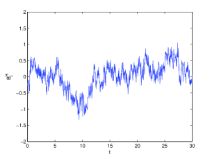
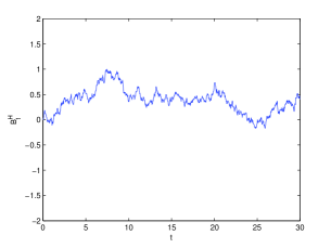
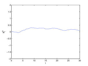
For H = 1/2, the fBM is then a standard Brownian motion. Hence, in this case the increments of the process are independent. On the contrary, for $H\neq 1/2$ the increments are not independent. More precisely, by the definition of fBM, we know that the covariance between $B^{H}(t+h)-B^{H}(t)$ and $B^{H}(s+h)-B^{H}(s)$ with $s+h\leq t$ and $t-s=nh$ is

$$\rho_{H}(n)=\frac{1}{2}h^{2H}[(n+1)^{2H}+(n-1)^{2H}-2n^{2H}].$$

In particular, we obtain that the two increments of the form $B^{H}(t+h)-B^{H}(t)$ and $B^{H}(t+2h)-B^{H}(t+h)$ are positively correlated for $H>1/2$, while they are negatively correlated for $H<1/2$. In the first case the process presents an aggregation behavior and this property can be used in order to describe ”cluster” phenomena (systems with memory and persistence). In the second case it can be used to model sequences with intermittency and antipersistence.

From the above description, we can get a general ideal that the Hurst parameter H plays an important role on how respective fBM behaves. So, it should be considered as an extra parameter when we estimate others in the coefficients of the SDE driven by fBM.

Considering the further computation, we would like to introduce one more useful property of fBM.

Definition 3.2 (Self-similarity).

A stochastic process X$=\{X_{t},t\in{\mathbb{R}}\}$ is called b-self-similar or satisfies the property of self-similarity if for every $a>0$ there exists $b>0$ such that

$$Law(X_{at},t\geq 0)=Law(a^{b}X_{t},t\geq 0).$$

Note that ’Law=Law’ means that the two processes $X_{at}$ and $a^{b}X_{t}$ have the same finite-dimensional distribution functions, i.e., for every choice $t_{0},\ldots,t_{n}$ in ${\mathbb{R}}$,

$$P(X_{at_{0}}\leq x_{0},\ldots,X_{at_{n}}\leq x_{n})=P(a^{b}X_{t_{0}}\leq x_{0},\ldots,a^{b}X_{t_{n}}\leq x_{n}).$$

for every $x_{0},\ldots,x_{n}$ in ${\mathbb{R}}$.

Since the covariance function of the fBM is homogeneous of order 2H, we obtain that $B^{H}$ is a self-similar process with Hurst index H, i.e., for any constant $a>0$, the processes $B^{H}(at)$ and $a^{H}B^{H}(t)$ have the same distribution law.

3.2. How to Estimate Hurst Parameter $H$

Let’s start with the simplest case:

$$dX_{t}=dB^{H}(t),~{}~{}~{}~{}~{}~{}~{}~{}~{}~{}~{}~{}~{}i.e.,X_{t}=B^{H}(t)~{}~{}~{}~{}~{}~{}~{}~{}~{}~{}t\geq 0,$$

where $\{B^{H}(t),t\geq 0\}$ is a fBM with Hurst parameter $H\in(0,1)$. Now, our question is how to estimate Hurst parameter H given observation data $X_{0},X_{1},\ldots,X_{N}$. For a parameter estimation of Hurst parameter H, we need an extra ingredient, fractional Gaussian noise (fGn).

Definition 3.3 (Fractional Gaussian noise).

[110]
Fractional Gaussian noise (fGn) $\{Y_{i},i\geq 1\}$ is the increment of fractional Brownian motion, namely

$$Y_{i}=B^{H}(i+1)-B^{H}(i),~{}~{}~{}~{}~{}~{}~{}~{}~{}~{}~{}~{}~{}i\geq 1.$$

Remark: It is a mean zero, stationary Gaussian time series whose autocovariance function is given by

$$\rho(h)=E(Y_{i}Y_{i+h})=\frac{1}{2}\{(h+1)^{2H}-2h^{2H}+|h-1|^{2H}\},~{}~{}~{}h\geq 0.$$

An important point about $\rho(h)$ is

$$\rho(h)\sim H(2H-1)h^{2H-2},~{}~{}~{}~{}as~{}~{}~{}h\rightarrow\infty,$$

when $H\neq 1/2$. Since $\rho(h)=0$ for $h\geq 1$ when H=1/2, the $X_{i}$’s are white noise in this case. The $X_{i}$’s, however, are positively correlated when $\frac{1}{2}<H<1$, and we say that they display long-range dependence (LRD) or long memory.

From the expression of fGn, we know it is the same to estimate the Hurst parameter of fBM as to estimate the Hurst parameter of the respective fGn. Here, we introduce 4 different methods for measuring the Hurst parameter. Measurements are given on artificial data and the results of each method are compared in the end. However, the measurement techniques used in this paper can only be described briefly but references to fuller descriptions with mathematical details are given.

3.2.1. R/S Method

The R/S method is one of the oldest and best known techniques for estimating H. It is discussed in detail in [83] and [10], p.83-87.

For a time series $\{Y_{t}:t=1,2,\ldots,N\}$ with partial sums given by $Z(n)=\sum^{n}_{i=1}Y_{i}$ and the sample variance given by

$$S^{2}(n)=\frac{1}{n-1}\sum^{n}_{i=1}Y^{2}_{i}-\frac{1}{n(n-1)}Z(n)^{2},$$

then the R/S statistic, or the rescaled adjusted range, is given by:

$$\frac{R}{S}(n)=\frac{1}{S(n)}\left[\max_{1\leq t\leq n}\left(Z(t)-\frac{t}{n}Z(n)\right)-\min_{1\leq t\leq n}\left(Z(t)-\frac{t}{n}Z(n)\right)\right]$$

For fractional Gaussian noise,

$$E[R/S(n)]\sim C_{H}n^{H},$$

as $n\rightarrow\infty$, where $C_{H}$ is another positive, finite constant not dependent on n.

The procedure to estimate H is therefore as follows. For a time series of length N, subdivide the series into K blocks with each of size $n=N/K$. Then, for each lag n, compute $R/S(k_{i},n)$, starting at points $k_{i}=iN/K+1,i=1,2,\ldots,K-1.$ In this way, a number of estimates of $R/S(n)$ are obtained for each value of n. For values of n approaching N, one gets fewer values, as few as 1 when $n\geq N-N/K$.

Choosing logarithmically spaced values of n, plot $\log[R/S(k_{i},n)]$ versus $\log n$ and get, for each n, several points on the plot. This plot is sometimes called the pox plot for the R/S statistic. The parameter H can be estimated by fitting a line to the points in the pox plot.

There are several disadvantages with this technique. Most notably, there are more estimates of the statistic for low values of n where the statistic is affected most heavily by short range correlation behavior. On the other hand, for high values of n there are too few points for a reliable estimate. The values between these high and low cut off points should be used to estimate H but, in practice, often it is the case that widely differing values of H can be found by this method depending on the high and low cut off points chosen. To modify the R/S statistic, we can use a weighted sum of autocovariance instead of the sample variance. Details can be found in [82].

3.2.2. Aggregated Variance.

Given a time series $\{Y_{t}:t=1,2,\ldots,N\}$, divide this into blocks of length m and aggregate the series over each block.

$$Y^{(m)}(k):=\frac{1}{m}\sum^{km}_{i=(k-1)m+1}Y_{i},~{}~{}~{}~{}~{}k=1,2,...,[N/m].$$

We compute its sample variance,

$$\widehat{VarY^{(m)}}=\frac{1}{N/m}\sum^{N/m}_{k=1}(Y^{(m)}(k)-\overline{Y})^{2}.$$

where

$$\overline{Y}=\frac{\sum^{N}_{i=1}Y_{i}}{N}.$$

is the sample mean. The sample variance should be asymptotically proportional to $m^{2H-2}$ for large $N/m$ and m. Then, for successive values of m, the sample variance of the aggregated series is plotted versus m on a log-log plot. So we can get the estimate of H by computing the gradient of that log-log plot. However, jumps in the mean and slowly decaying trends can severely affect this statistic. One technique to combat this is to difference the aggregated variance and work instead with

$$\widehat{VarY^{(m+1)}}-\widehat{VarY^{(m)}}.$$

3.2.3. Variance of Residuals.

This method is described in more detail in [101]. Take the series $\{Y_{t}:t=1,2,\ldots,N\}$ and divide it into blocks of length m. Within each block calculate partial sums: $Z_{k}(t)=\sum^{(k-1)m+t}_{i=(k-1)m+1}Y_{i}$, $k=1\ldots N/m,~{}t=1\ldots m$. For each block make a least squares fit to a line $a_{k}+b_{k}t$. Subtract this line from the samples in the block to obtain the residuals and then calculate their variance

$$V_{k}=\frac{1}{m}\sum^{m}_{t=1}(Z_{k}(t)-a_{k}-b_{k}t)^{2}.$$

The variance of residuals is proportional to $m^{2H}$. For the proof in the Gaussian case, see [118]. This variance of residuals is computed for each block, and the median (or average) is computed over the blocks. A log-log plot versus m should follow a straight line with a slope of 2H.

3.2.4. Periodogram.

The periodogram is a frequency domain technique described in [49]. For a time series $\{Y_{t}:t=1,2,\ldots,N\}$, it is defined by

$$I(\lambda)=\frac{1}{2\pi N}\left|\sum^{N}_{j=1}Y_{j}e^{ij\lambda}\right|^{2},$$

where $\lambda$ is the frequency. In the finite variance case, $I(\lambda)$ is an estimate of the spectral density of Y, and a series with long-range dependence will have a spectral density proportional to $|\lambda|^{1-2H}$ for frequencies close to the origin. Therefore, the log-log plot of the periodogram versus the frequency displays a straight line with a slope of 1-2H.

3.2.5. Results on Simulated Data

In this subsection, we would like to use artificial data to check the robustness of above techniques and compare the result in the end.

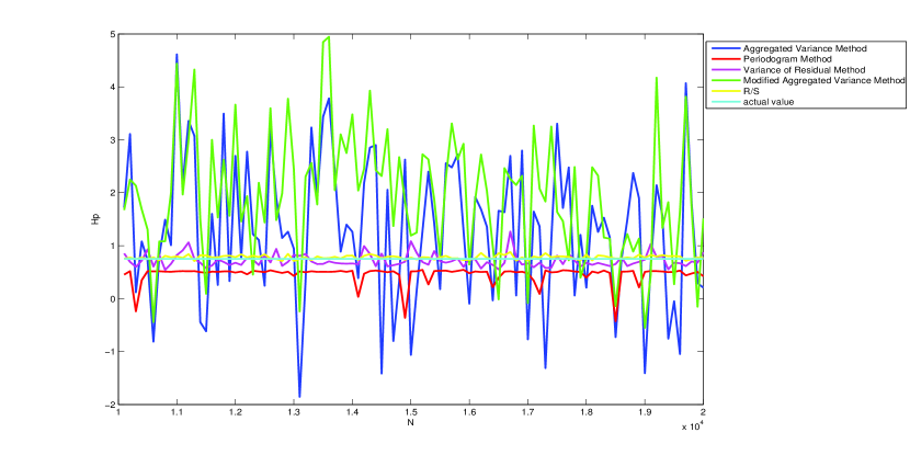
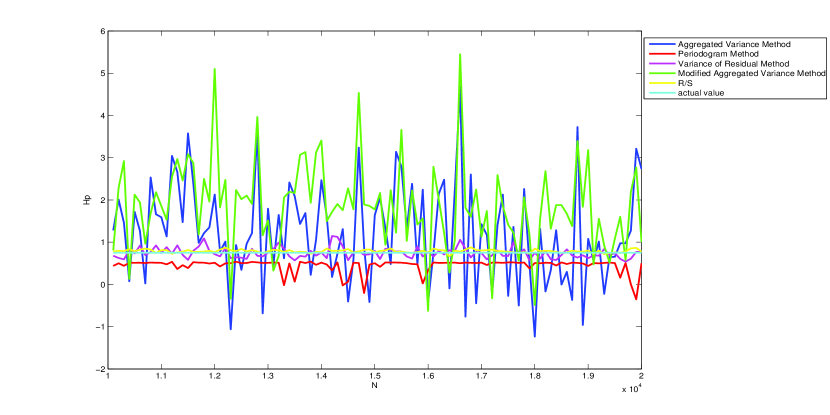
For each of the simulation methods chosen, traces have been generated. Each trace is 10,000 points of data. Hurst parameters of 0.65 and 0.95 have been chosen to represent a low and a high level of long-range dependence in data. From the Figure 2 and Figure 3, we can see that the Variance of Residual Method and R/S have the most accurate result. The Modified Aggregated Variance Method improved a little bit over the original one, but both of them still fluctuate too much.

Figure 2. Numerical estimation of the Hurst parameter $H$ of fBM: Actual value $H=0.65$

Figure 3. Numerical estimation of the Hurst parameter $H$ of fBM: Actual value $H=0.95$

3.3. How to Estimate Parameters in SDEs Driven by fBM

After we discuss how to estimate the Hurst parameter of a series of artificial fBM data, now we want to concern how to estimate the parameters of the linear/nonlinear stochastic differential equation(s) driven by fBM. The coefficients in the stochastic differential equation could be deterministic or random, linear or nonlinear. No general results are available. So some specific statistical results will be discussed below according to what kind of specified models we deal with.

3.3.1. Preparation

The main difficulty in dealing with a fBm is that it is not a semimartingale when $H\neq\frac{1}{2}$ and hence the results from the classical stochastic integration theory for semimartingales can not be applied. So, we would like to introduce the following integral transformation which can transform fBM to martingale firstly and it will be a key point in our development below. For $0<s<t\leq T$, denote

(14) $$k_{H}(t,s) = \kappa^{-1}_{H}s^{(1/2)-H}(t-s)^{(1/2)-H},$$

(15) $$\kappa_{H} = 2H\Gamma(3/2-H)\Gamma(H+1/2),$$

(16) $$w^{H}_{t} = \lambda^{-1}_{H}t^{2-2H};~{}~{}~{}~{}~{}\lambda_{H}=\frac{2H\Gamma(3-2H)\Gamma(H+1/2)}{\Gamma(3/2-H)},$$

(17) $$M^{H}_{t} = \int^{t}_{0}k_{H}(t,s)dB^{H}_{s}.$$

Then the process $M^{H}$ is a Gaussian martingale (see [78] and [92]), called the fundamental martingale with variance function $w^{H}$.

3.3.2. Parameter Estimation for a Fractional Langevin Equation

Suppose $\{X_{t},~{}t\geq 0\}$ satisfies the following stochastic differential equation

$$X_{t}=\theta\int^{t}_{0}X_{s}ds+\sigma B^{H}_{t};~{}~{}~{}~{}~{}~{}~{}~{}~{}0\leq t\leq T,$$

where $\theta$ and $\sigma^{2}$ are unknown constant parameters, $B^{H}_{t}$ is a fBM with Hurst parameter $H\in[1/2,1]$.

Denote the process Z=$(Z_{t},t\in[0,T])$ by

(18) $$Z_{t}=\int^{t}_{0}k_{H}(t,s)dX_{s}.$$

Then we can prove that process Z is a semimartingale associated to X with following decomposition (see [69])

(19) $$Z_{t}=\theta\int^{t}_{0}Q(s)dw^{H}_{s}+\sigma M^{H}_{t},$$

where

(20) $$Q(t)=\frac{d}{dw^{H}_{t}}\int^{t}_{0}k_{H}(t,s)X(s)ds,$$

and $M^{H}_{t}$is the Gaussian martingale defined by (17). From the representation (19), we know the quadratic variation of Z on the interval [0, t] is nothing but

$$\langle Z\rangle_{t}=\sigma^{2}w^{H}_{t},~{}~{}~{}~{}~{}~{}a.s.$$

Hence the parameter $\sigma^{2}$ can be obtained by

$$[w^{H}_{t}]^{-1}\lim_{n}\sum_{i}\left[Z_{t^{n}_{i+1}}-Z_{t^{n}_{i}}\right]^{2}=\sigma^{2},~{}~{}~{}~{}~{}~{}a.s.$$

where $t^{n}_{i}$ is an appropriate partition of [0,t] such that $\sup_{i}|t^{n}_{i+1}-t^{n}_{i}|\rightarrow 0$ as $n\rightarrow\infty$. So, the variance parameter can be computed with probability 1 on any finite time interval.

As for the parameter $\theta$, by applying the Girsanov type formula for fBM which is proved in [69], we can define the following maximum likelihood estimate of $\theta$ based on the observation on the interval [0, t] by

(21) $$\theta_{T}=\left\{\int^{T}_{0}Q^{2}(s)dw^{H}_{s}\right\}^{-1}\int^{T}_{0}Q(s)dZ_{s},$$

where processes Q, Z and $w^{H}_{t}$ are defined by (20), (18) and (16), respectively. For this estimate, strong consistency is proven and explicit formulas for the asymptotic bias and mean square error are derived by Kleptsyna and Le Breton [70].

Remarks:

• When $H=1/2$, since $Q=Z=X$ and $d\omega_{s}^{1/2}=ds$, the formula (21) reduces to the result of [80] for an usual Ornstein-Uhlenbeck process.

• For an arbitrary $H\in[1/2,1]$, we could derive the following alternative expression for $\theta_{T}$:

  $$\theta_{T}=\left\{2\int^{T}_{0}Q^{2}(s)dw^{H}_{s}\right\}^{-1}\left\{\frac{\lambda_{H}}{2-2H}Z_{T}\int^{T}_{0}s^{2H-1}dZ_{s}-t\right\}.$$

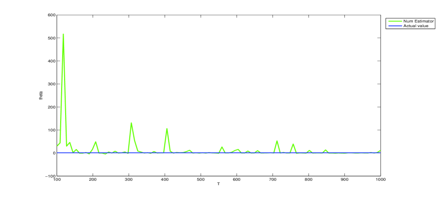
Example 3.4.

Consider a special Ornstein-Uhlenbeck model

$$dX_{t}=\theta X_{t}dt+2dB^{H}_{t}.$$

Then, according to the above approximation scheme, we can numerically estimate $\theta=1$ and the results are shown in Figure 4.

Figure 4. Numerical estimation of drift parameter $\theta$ in $dX_{t}=\theta X_{t}dt+2dB^{H}_{t}$ with Hurst parameter $H=0.75$: Actual value $\theta_{0}=1$

3.3.3. Parameter Estimation in Linear Deterministic Regression

Suppose $X_{t}$ satisfies the following stochastic differential equation

$$X_{t}=\theta\int^{t}_{0}A(s)ds+\int^{t}_{0}C(s)dB^{H}_{s},~{}~{}~{}~{}~{}~{}~{}~{}~{}0\leq t\leq T,$$

where A and C are deterministic measurable functions on [0,T], $B^{H}_{t}$ is a fBM with Hurst parameter $H\in[1/2,1]$.

Let $q_{t}$ be defined by

$$q_{t}=\frac{d}{dw^{H}_{t}}\int^{t}_{0}k_{H}(t,s)\frac{A}{C}(s)ds,$$

where $w^{H}_{t}$ and $k_{H}(t,s)$ are defined by (16) and (14). Then, from Theorem 3 in [69], we obtain the maximum likelihood estimate of $\theta$ defined by

$$\theta_{T}=\left\{\int^{T}_{0}q^{2}_{t}dw^{H}_{t}\right\}^{-1}\int^{T}_{0}q_{t}dZ_{t},$$

where $Z_{t}$ is defined by (18).

Remark: This result can be extended to an arbitrary H in (0,1) (see [78]) and $\theta_{T}$ is also the best linear unbiased estimate of $\theta$.

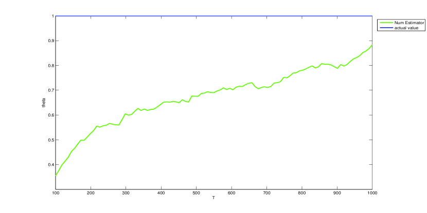
Example 3.5.

Consider a special Linear Deterministic Regression

$$dX_{t}=-\theta dt+tdB^{H}_{t}.$$

Then, using the above estimate, we can do numerical simulation with result shown in Figure 5.

Figure 5. Numerical estimation of drift parameter $\theta$ in a Linear Deterministic Regression $dX_{t}=-\theta dt+tdB^{H}_{t}$ with Hurst parameter $H=0.75$: Actual value $\theta$=1

3.3.4. Parameter Estimation in Linear Random Regression

Let us consider a stochastic differential equation

$$\d{X}(t)=[A(t,X(t))+\theta C(t,X(t))]dt+\sigma(t)dB^{H}_{t},~{}~{}~{}t\geq 0,$$

where $B=\{B^{H}_{t},t\geq 0\}$ is a fractional Brownian motion with Hurst parameter H and $\sigma(t)$ is a positive nonvanishing function on $[0,\infty)$. According to [105], the Maximum Likelihood Estimate $\hat{\theta}_{T}$ of $\theta$ is given by

$$\theta_{T}=\frac{\int^{T}_{0}J_{2}(t)dZ_{t}+\int^{T}_{0}J_{1}(t)J_{2}(t)dw^{H}_{t}}{\int^{T}_{0}J^{2}_{2}(t)dw^{H}_{t}},$$

where the processes $Z_{t},J_{1},J_{2}$ are defined by

$$Z_{t} = \int^{t}_{0}\frac{k_{H}(t,s)}{\sigma(s)}dX_{s},t\geq 0,$$

$$J_{1}(t) = \frac{d}{dw^{H}_{t}}\int^{t}_{0}k_{H}(t,s)\frac{A(s,X(s))}{\sigma(s)}ds,~{}~{}~{}~{}~{}J_{2}(t)=\frac{d}{dw^{H}_{t}}\int^{t}_{0}k_{H}(t,s)\frac{C(s,X(s))}{\sigma(s)}ds,$$

and $w^{H}_{t}$, $k_{H}(t,s)$ are defined by (16) and (14). Also in the same paper, they proved that $\theta_{T}$ is strongly consistent for the true value $\theta$.

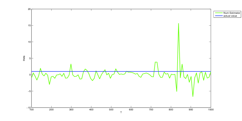
Example 3.6.

Consider a special Linear Random Regression

$$dX_{t}=(t+\theta X_{t})dt+tdB^{H}_{t}.$$

A numerical estimation of the parameter $\theta$ is shown in Figure 6.

Figure 6. Numerical estimation of drift parameter $\theta$ in a Linear Random Regression $dX_{t}=(t+\theta X_{t})dt+tdB^{H}_{t}$ with Hurst parameter $H=0.75$: Actual value $\theta$=1

4. Parameter Estimation for SDE Driven by $\alpha$-Stable Lévy Motion

Brownian motion, as a Gaussian process, has been widely used to model fluctuations in engineering and science. For a particle in Brownian motion, its sample paths are continuous in time almost surely (i.e., no jumps), its mean square displacement increases linearly in time (i.e., normal diffusion), and its probability density function decays exponentially in space (i.e., light tail or exponential relaxation) [95]. However some complex phenomena involve non-Gaussian fluctuations, with properties such as anomalous diffusion (mean square displacement is a nonlinear power law of time) [15] and heavy tail (non-exponential relaxation) [129]. For instance, it has been argued that diffusion in a case of geophysical turbulence [114] is anomalous. Loosely speaking, the diffusion process consists of a series of “pauses”, when the particle is trapped by a coherent structure, and “flights” or “jumps” or other extreme events, when the particle moves in a jet flow. Moreover, anomalous electrical transport properties have been observed in some amorphous materials such as insulators, semiconductors and polymers, where transient current is asymptotically a power law function of time [112, 53]. Finally, some paleoclimatic data [29] indicates heavy tail distributions and some DNA data [114] shows long range power law decay for spatial correlation. Lévy motions are thought to be appropriate models for non-Gaussian processes with jumps [111]. Here we consider a special non-Gaussian process, the $\alpha$-stable Lévy motion, which arise in many complex systems [126].

4.1. $\alpha$-Stable Lévy Motion

There are several reasons for using a stable distribution to model a fluctuation process in a dynamical system. Firstly, there are theoretical reasons for expecting a non-Gaussian stable model, e.g. hitting times for a Brownian motion yielding a Lévy distribution, and reflection off a rotating mirror yielding a Cauchy distribution. The second reason is the Generalized Central Limit Theorem which states that the only possible non-trivial limit of normalized sums of i.i.d. terms is stable. The third argument for modeling with stable distributions is empirical: Many large data sets exhibit heavy tails and skewness. In this section, we consider one-dimensional $\alpha$-stable distributions defined as follows.

Definition 4.1.

([64], Chapter 2.4) The Characteristic Function $\varphi(u)$ of an $\alpha$-stable random variable is given by

(22) $$\varphi(u)=\exp((-\sigma^{\alpha})|u|^{\alpha}\{1-i\beta sgn(u)\tan(\alpha\pi/2)\}+i\mu u)$$

where $\alpha\in(0,1)\cup(1,2),~{}\beta\in[-1,1],\sigma\in{\mathbb{R}}_{+},~{}\mu\in{\mathbb{R}}$, and by

(23) $$\varphi(u)=\exp(-\sigma|u|\{1+i\beta\frac{2}{\pi}sgn(u)\log(|u|)\}+i\mu u)$$

when $\alpha=1$, it gives a very well-known symmetric Cauchy distribution and

(24) $$\varphi(u)=\exp(-\frac{1}{2}\sigma|u|^{2}+i\mu u),$$

when $\alpha=2$, it gives the well-known Gaussian distribution.

For the random variable X distributed according to the rule described above we use the notation $X\thicksim S_{\alpha}(\sigma,\beta,\mu)$. Especially when $\mu=\beta=0$, i.e., X is a symmetric $\alpha$-stable random variable, we will denote it as $X\thicksim S\alpha S$.

Also, from above definition, it is easy to see that the full stable class is characterized by four parameters, usually designated $\alpha,\beta,\sigma,$ and $\mu$. The shift parameter $\mu$ simply shifts the distribution to the left or right. The scale parameter $\sigma$ compresses or extends the distribution about $\mu$ in proportion to $\sigma$ which means, if the variable x has the stable distribution $X\thicksim S_{\alpha}(\sigma,\beta,\mu)$, the transformed variable $z=(x-\mu)/\sigma$ will have the same shaped distribution, but with location parameter 0 and scale parameter 1. The two remaining parameters completely determine the distribution’s shape. The characteristic exponent $\alpha$ lies in the range $(0,2]$ and determines the rate at which the tails of the distribution taper off. When $\alpha=2$, a normal distribution results. When $\alpha<2$, the variance is infinite. When $\alpha>1$, the mean of the distribution exists and is equal to $\mu$. However, when $\alpha\leq 1$, the tails are so heavy that even the mean does not exist. The fourth parameter $\beta$ determines the skewness of the distribution and lies in the range [-1,1].

Now let us introduce $\alpha$-stable L$\acute{e}$vy motions.

Definition 4.2.

($\alpha$-stable L$\acute{e}$vy motion [64])
A stochastic process $\{X(t):t\geq 0\}$ is called the (standard) $\alpha$-stable L$\acute{e}$vy motion if

1. X(0)=0 a.s.;

2. $\{X(t):t\geq 0\}$ has independent increments;

3. X(t)-X(s)$\thicksim S_{\alpha}((t-s)^{1/\alpha},\beta,0)$ for any $0\leq s<t<\infty$.

So, from the third condition, we can simulate all $\alpha$-stable L$\acute{e}$vy motion if we know how to simulate $X\thicksim S_{\alpha}(\sigma,\beta,0)$. Especially, it is enough to simulate $X\thicksim S_{\alpha}(\sigma,0,0)$ if we want to get the trajectories of symmetric $\alpha$-stable L$\acute{e}$vy motions.

We recall an important property of $\alpha$-Stable random variables giving us the following result: It is enough to know how to simulate $X\thicksim S_{\alpha}(1,0,0)$ in order to get any $X\thicksim S_{\alpha}(\sigma,0,0),\forall\sigma\in{\mathbb{R}}^{+}$.

Proposition 4.3.

If we have $X_{1},X_{2}\thicksim S_{\alpha}(\sigma,\beta,\mu)$ and A, B are real positive constants and C is a real constant, then

$$AX_{1}+BX_{2}+C\thicksim S_{\alpha}(\sigma(A^{\alpha}+B^{\alpha})^{1/\alpha},\beta,\mu(A^{\alpha}+B^{\alpha})^{1/\alpha}+C)\\$$

Proposition 4.4.

Let $X\sim S_{\alpha}(\sigma,\beta,0)$, with $0<\alpha<2$, Then $E|X|^{p}<\infty$ for any $0<p<\alpha$, $E|X|^{p}=\infty$ for any $p\geq\alpha.$

Figure 7 shows sample paths of the $\alpha$-stable Lévy motion with different $\alpha$.

Figure 7. Three sample paths of symmetric $\alpha-$stable Lévy motion with $\alpha=0.4,1.2,1.9$, respectively

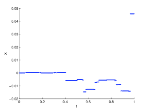
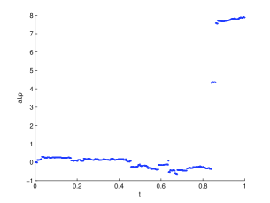
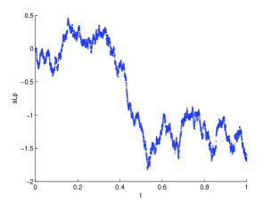
As we can see in Figure 7, the bigger the parameter $\alpha$ is, the more the path looks like Brownian motion. Generally speaking, when we deal with concrete data, we have to choose $\alpha$-stable processes very carefully to get the best estimation. We now discuss how to estimate $\alpha$.

4.2. How to Estimate the Characteristic Exponent $\alpha$

Five different methods about how to estimate the characteristic exponent $\alpha$ of $\alpha-$stable distribution are considered: Characteristic Function Method(CFM), Quantile Method, Maximum Likelihood Method, Extreme Value Method and Moment Method. As in the last section, measurements are given on artificial data and the results of each method are compared in the end of this section.

4.2.1. Characteristic Function Method

Since $\alpha-$stable distributions are uniquely determined by their Characteristic Function (CF), it is natural to consider how to estimate parameter by studying their CF. Press [106] introduced a parameter estimation method based on CF, which gets estimations of parameters by minimizing differences between values of sample CF and the real ones. But this method is only applicable to standard distributions.

Another method which uses the linearity of logarithm of CF was developed by Koutrouvelis [74] and it can be applied to general $\alpha$-stable cases. This method is denoted as Kou-CFM. The idea is as follows: On the one hand, taking the logarithm of real part of CF gives

$$\ln[-Re(\varphi(u))]=\alpha\ln|u|+\alpha\ln\sigma.$$

On the other hand, the sample characteristic function of $\varphi(\theta)$ is given by $\Phi(\theta)=(\sum^{N}_{k=1}e^{i\theta y_{k}})$ where $y_{k}$’s are $n$ independent observations. In [74], a regression technique is applied to gain estimates for all parameters of a observed $\alpha$ stable distribution. In [72], Kogon improved this method by replacing a linear regression fit by a linear least square fit which gave a more accurate estimate and its computational complexity became lower.

4.2.2. Quantile Method

Quantiles are points taken at regular intervals from the cumulative distribution function of a random variable. Suppose we have $n$ independent symmetric $\alpha$-stable random variables with the stable distribution $S_{\alpha}(\sigma,\beta,\mu)$, whose parameters are to be estimated. Let $x_{p}$ be the p-th quantile, so that $S_{\alpha}(x_{p};\sigma,\beta,\mu)=p$. Let $\hat{x_{p}}$ be the corresponding sample quantile, then $\hat{x_{p}}$ is a consistent estimate of $x_{p}$.

In 1971, Fama and Roll [41] discovered that, for some large p (for example, p=0.95),

$$\hat{z}_{p}=\frac{\hat{x}_{p}-\hat{x}_{1-p}}{2\sigma}=(0.827)\frac{\hat{x}_{p}-\hat{x}_{1-p}}{\hat{x}_{0.72}-\hat{x}_{0.28}}$$

is an estimate of the p-quantile of the standardized symmetric stable distribution with exponent $\alpha$. According to this, they proposed a estimate (QM) for symmetric $\alpha$-stable distributions. However, the serious disadvantage of this method is that its estimations are asymptotically biased.
Later on, McCulloch [87] improved and extended this result to general $\alpha$-stable distributions, denoted as McCulloch-QM. Firstly, he defined

$$v_{\alpha} = (x_{-0.95}-x_{-0.05})/(x_{-0.75}-x_{-0.25})$$

$$v_{\beta} = (x_{-0.95}+x_{-0.05}-2x_{0.5})/(x_{-0.95}-x_{-0.05})$$

and let $\hat{v}_{\alpha}$ and $\hat{v}_{\beta}$ be the corresponding sample value:

$$\hat{v}_{\alpha} = (\hat{x}_{-0.95}-\hat{x}_{-0.05})/(\hat{x}_{-0.75}-\hat{x}_{-0.25})$$

$$\hat{v}_{\beta} = (\hat{x}_{-0.95}+\hat{x}_{-0.05}-2\hat{x}_{0.5})/(\hat{x}_{-0.95}-\hat{x}_{-0.05})$$

which are the consistent estimates of the index $v_{\alpha}$ and $v_{\beta}$. Then, he illustrated that estimates of $\alpha$ can be expressed by a function of $\hat{v}_{\alpha}$ and $\hat{v}_{\beta}$. Compared with QM, McCulloch-QM could get consistent and unbiased estimations for the general $\alpha$-stable distribution, and extend the estimation range of parameter $\alpha$ to $0.6\leq\alpha\leq 2$. Despite its computational simplicity, this method has a number of drawbacks, such as, there are no analytical expressions for the value of the fraction, and the evaluation of the tables implies that it is highly dependent on the value of $\alpha$ in a nonlinear way. This technique does not provide any closed-form solutions.

4.2.3. Extreme Value Method

In 1996, based on asymptotic extreme value theory, order statistics and fractional lower order moments, Tsihrintzis and Nikias [119] proposed a new estimate which can be computed fast for symmetric $\alpha$ stable distribution from a set of i.i.d. observations. Five years later, Kuruoglu [76] extended it to the general $\alpha$ stable distributions. The general idea of this method is as follows. Given a data series $\{X_{i}:i=1,2,\ldots,N\}$, divide this into L nonoverlapping blocks of length K such that $K=N/L$. Then the logarithms of the maximum and minimum samples of each segment are computed as follows

$$\overline{Y_{l}} = \log(\max\{X_{lK-K+i}|i=1,2,\ldots,K\}),$$

$$\underline{Y_{l}} = \log(-\min\{X_{lK-K+i}|i=1,2,\ldots,K\}).$$

The sample means and variances of $\overline{Y_{l}}$ and $\underline{Y_{l}}$ are calculated as

$$\overline{Y} = \frac{1}{L}\sum^{L}_{l=1}\overline{Y_{l}},~{}~{}~{}~{}~{}\overline{s^{2}}=\frac{1}{L-1}\sum^{L}_{l=1}(\overline{Y_{l}}-\overline{Y})^{2},$$

$$\underline{Y} = \frac{1}{L}\sum^{L}_{l=1}\underline{Y_{l}},~{}~{}~{}~{}~{}\underline{s^{2}}=\frac{1}{L-1}\sum^{L}_{l=1}(\underline{Y_{l}}-\underline{Y})^{2}.$$

Finally, an estimate for $\alpha$ is given by sample variance as follows

$$\hat{\alpha}=\frac{\pi}{2\sqrt{6}}\left(\frac{1}{\overline{s}}+\frac{1}{\underline{s}}\right).$$

Even though the accuracy and computational complexity decrease, there is now a closed form for the block size which means we have to look-up table to determine the segment size K.

4.2.4. Moment Estimation Method

Another way to estimate parameters of the general $\alpha$-stable distribution is the Logarithmic Moments Methods which was also introduced by Kuruoglu [76]. The advantage of this method relative to the Fractional Lower Order Method is that it does not require the inversion of a sinc function or the choice of a moment exponent p. The main feature is that the estimate of $\alpha$ can be expressed by a function of the second-order moment of the skewed process, i.e.

$$\hat{\alpha}=\left(\frac{L_{2}}{\psi_{1}}-\frac{1}{2}\right)^{-1/2},$$

where $\psi_{1}=\frac{\pi^{2}}{6}$ and, for any $X\sim S_{\alpha}(\sigma,\beta,0)$, $L_{2}$ is defined as follows

$$L_{2}=E[(\log|X|-E[\log|X|])^{2}]=\psi_{1}\left(\frac{1}{2}+\frac{1}{\alpha^{2}}\right)-\frac{\theta^{2}}{\alpha^{2}}.$$

4.2.5. Results on Simulated Data

In this subsection, we would like to use artificial data to check the robustness of the above techniques and compare the results.

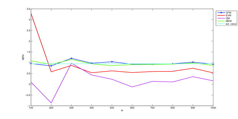
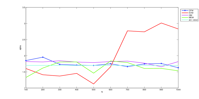
For each of the simulation methods chosen, estimates of $\alpha$ have been generated respectively and each trace is 1,000 points of data. Characteristic exponents of 0.95 and 1.70 have been chosen to represent a low and a high level of the rate at which the tails of the distribution taper off.

From the Figures 8 and 9, we can see that the Characteristic Function Method and the Moment Estimate Method have the most accurate result. The Quantile Method behaved a little better than Extreme Value Method, but both of them still fluctuate too much when $\alpha$ is small. As to the convergence, we can see that all the methods get closer and closer to the real value when the points of data increase except for the Extreme Value Method.

Figure 8. Numerical estimation of the characteristic exponent $\alpha$ in the $\alpha-$stable Lévy motion $L_{t}^{\alpha}$ by 4 different methods: Actual value $\alpha=0.95$

Figure 9. Numerical estimation of the characteristic exponent $\alpha$ in the $\alpha-$stable Lévy motion $L_{t}^{\alpha}$ by 4 different methods: Actual value $\alpha=1.70$

4.3. How to Estimate Parameters in SDEs Driven by Lévy Motion

After we discussed how to estimate the characteristic exponent of $\alpha$-stable Lévy motions, now we consider how to estimate the parameters in stochastic differential equations driven by general Lévy motion. Just as what we discussed about fBM, no general results about the parameter estimation for general cases are available at this time. Some special results will be listed below for different equations.

We consider parameter estimation of the Lévy-driven stationary Ornstein-Uhlenbeck process. Recently, Brockdwell, Davis and Yang [16] studied parameter estimation problems for Lévy-driven Langevin equation (whose solution is called an Ornstein-Uhlenceck process) based on observations made at uniformly and closely-spaced times. The idea is to obtain a highly efficient estimate of the Lévy-driven Ornstein-Uhlenceck process coefficient by estimating the corresponding coefficient of the sampled process. The main feature is discussed below.

Consider a stochastic differential equation driven by the Lévy motion $\{L(t),t\geq 0\}$

$$dY(t)=-\theta Y(t)dt+\sigma dL(t).$$

When $L(t)$ is Brownian motion, the solution of above equation can be expressed as

(25) $$Y(t)=e^{-\theta t}Y(0)+\sigma\int^{t}_{0}e^{-\theta(t-u)}dL(t).$$

For any second-order driving Lévy motion, the process $\{Y(t)\}$ can be defined in the same way, and if $\{L(t)\}$ is non-decreasing, $\{Y(t)\}$ can also be defined pathwise as a Riemann-Stieltjes integral by (25). For the convenience of the simulation, we rewrite solution as follows

(26) $$Y(t)=e^{-\theta(t-s)}Y(s)+\sigma\int^{t}_{s}e^{-\theta(t-u)}dL(u),~{}~{}for~{}all~{}t>s\geq 0.$$

Now we collect all information corresponding to the sampled process in order to get the estimate. Set $t=nh$ and $s=(n-1)h$ in equation (26). Then the sampled process $\{Y^{(h)}_{n},n=0,1,2,\ldots\}$ (or the discrete-time AR(1) process) satisfies

$$Y^{(h)}_{n}=\varphi Y^{(h)}_{n-1}+Z_{n},$$

where

$$\varphi=e^{-\theta h},~{}~{}~{}and~{}~{}~{}Z_{n}=\sigma\int^{nh}_{(n-1)h}e^{-\theta(nh-u)}dL(u).$$

Then, using the highly efficient Davis-McCormick estimate of $\varphi$, namely

$$\hat{\varphi}^{(h)}_{N}=min_{1\leq n\leq N}\frac{Y^{(h)}_{n}}{Y^{(h)}_{n-1}},$$

we can get the estimate of $\theta$ and $\sigma$ as follows

$$\hat{\theta}^{(h)}_{N} = -h^{-1}\log\hat{\varphi}^{(h)}_{N},$$

$$\hat{\sigma}^{(2)}_{N} = \frac{2\hat{\theta}^{(h)}_{N}}{N}\sum^{N}_{i=0}(Y^{(h)}_{i}-\overline{Y}^{(h)}_{N})^{2}.$$

Example 4.5.

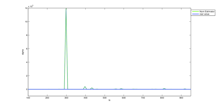
Consider a Lévy-driven Ornstein-Uhlenbeck process satisfying the following SDE

(27) $$dX_{t}=-X_{t}dt+\sigma dL^{\alpha}_{t}.$$

A numerical estimation of the diffusion parameter $\sigma$ is shown in Figure 10.

Figure 10. Numerical estimation of the diffusion parameter $\sigma$ in Lévy-driven Ornstein-Uhlenbeck process $dX_{t}=-X_{t}dt+\sigma dL^{\alpha}_{t}$ with $\alpha=0.95$: Actual value $\sigma=2$

References

- [1] Y. At-Sahalia (2002), Maximum-likelihood estimation of discretely-sampled diffusions: a closed-form approximation approach, Econometrica 70, 223-262.
- [2] Y. At-Sahalia and P. A. Mykland (2004), Estimators of diffusions with randomly spaced discrete observations: a general theory, The Annals of Statistics 32(5), 2186-2222
- [3] Y. At-Sahalia and P. A. Mykland (2003), The effects of random and discrete sampling when estimating continuous-time diffusions, Econometrica 71(2), 483-549.
- [4] S. Albeverrio, B. Rüdiger and J. L. Wu (2000), Invariant measures and symmetry property of Lévy type operators, Potential Analysis 13, 147-168.
- [5] S. Alizadeh, M. W. Brandt and F. X. Diebold (2002), Range-based estimation of stochastic volatility models, The Journal of Finance 57(3), 1047-1091.
- [6] D. Applebaum (2009), Lévy Processes and Stochastic Calculus, 2nd edition, Cambridge University Press, UK.
- [7] L. Arnold (1998), Random Dynamical Systems, Springer, New York.
- [8] O. E. Barndorff-Nielsen, T. Mikosch and S. I. Resnick (Eds.) (2001), Lévy Processes: Theory and Applications, Birkhäuser, Boston.
- [9] C. Bender (2003), An Ito formula for generalized functionals of a Fractional Brownian motion with arbitrary Hurst parameter, Stoch. Proc. Appl. 104, 81-106.
- [10] J. Beran (1994), Statistics for Long-Memory Processes, Chapman and Hall.
- [11] J. Bertoin (1998), Lévy Processes, Cambridge University Press, Cambridge, U.K..
- [12] P. Billingsley (1961), Statistical Inference for Markov Processes, Chicago University Press, Chicago.
- [13] J. P. N. Bishwal (2007), Parameter Estimation in Stochastic Differential Equations, Springer, New York.
- [14] D. Blomker and S. Maier-Paape (2003), Pattern formation below criticality forced by noise, Z. Angew. Math. Phys. 54(1), 1–25.
- [15] J. P. Bouchaud and A. Georges (1990), Anomalous diffusion in disordered media: Statistic mechanics, models and physical applications, Phys. Repts 195, 127-293.
- [16] P. J. Brockwell, R. A. Davis, and Y. Yang (2007), Estimation for nonnegative Lévy-driven Ornstein-Uhlenbeck processes, J. Appl. Probab. 44(4), 977-989.
- [17] T. Caraballo, J. Langa and J. C. Robinson (2001), A stochastic pitchfork bifurcation in a reaction-diffusion equation, R. Soc. Lond. Proc. Ser. A 457, 2041–2061.
- [18] B. Chen (2009), Stochastic dynamics of water vapor in the climate system, Ph.D. Thesis, Illinois Institute of Technology, Chicago, USA.
- [19] B. Chen and J. Duan (2009), Stochastic quantification of missing mechanisms in dynamical systems, In “Recent Development in Stochastic Dynamics and Stochastic Analysis”, Interdisciplinary Math, Sci. 8, 67-76.
- [20] A. Chronopoulou and F. Viens (2009), Hurst index estimation for self-similar processes with long-memory. In “Recent Development in Stochastic Dynamics and Stochastic Analysis”, J. Duan, S. Luo and C. Wang (Eds.), World Scientific.
- [21] J. M. Corcuera, D. Nualart, and J. H. C. Woerner (2006), Power variation of some integral fractional processes, Bernoulli, 12, 713-735.
- [22] J. M. Corcuera, D. Nualart and J. H. C. Woerner (2007), A functional central limit theorem for the realized power variation of integrated stable process, Stochastic Analysis and Applications 25, 169-186.
- [23] J. Coeurjolly (2001), Estimating the parameters of the Fractional Brwonian motion by discrete variations of its sample paths, Statistical Inference for Stochastic Processes 4, 199-227.
- [24] J. Coeurjolly (2000): Simulation and identification of the Fractional Brwonian motion: a bibliographical and comparative study, Journal of Statistical Software, American Statistical Association 5(07).
- [25] H. Crauel and F. Flandoli (1998), Additive noise destroys a pitchfork bifurcation, Journal of Dynamics and Differential Equations 10, 259-274.
- [26] D. Dacunha-Castelle adn D. Florens-Zmirou (1986), Estimation of the coefficients of a diffusion from discrete observations, 19, 263-284.
- [27] G. Da Prato and J. Zabczyk (1992), Stochastic Equations in Infinite Dimensions, Cambridge University Press.
- [28] M. Davis (2001), Pricing weather derivatives by marginal value, Quantitative Finance 1(3), 305-308.
- [29] P. D. Ditlevsen (1999), Observation of stable noise induced millennial climate changes from an ice record, Geophys. Res. Lett. 26, 1441-1444.
- [30] J. L. Doob (1953), Stochastic Processes, John Wiley, New York.
- [31] A. Du and J. Duan (2009), A stochastic approach for parameterizing unresolved scales in a system with memory, Journal of Algorithms & Computational Technology 3, 393-405.
- [32] J. Duan (2009), Stochastic modeling of unresolved scales in complex systems, Frontiers of Math. in China, 4, 425-436.
- [33] J. Duan (2009), Predictability in spatially extended systems with model uncertainty I & II, Engineering Simulation 2, 17-32 & 3 21-35.
- [34] J. Duan (2009), Predictability in nonlinear dynamical systems with model uncertainty, Stochastic Physics and Climate Modeling, T. N. Palmer and P. Williams (eds.), Cambridge Univ. Press, pp.105-132.
- [35] J. Duan, X. Kan and B. Schmalfuss (2009), Canonical sample spaces for stochastic dynamical systems, In “Perspectives in Mathematical Sciences”, Interdisciplinary Math. Sci. 9, 53-70.
- [36] J. Duan, C. Li and and X. Wang (2009), Modeling colored noise by Fractional Brownian motion, Interdisciplinary Math. Sci. 8, 119-130.
- [37] J. Duan and B. Nadiga (2007), Stochastic parameterization of large Eddy simulation of geophysical flows, Proc. American Math. Soc. 135, 1187-1196.
- [38] G. Dohnal (1987), On estimating the diffusion coefficient, J. Appl. Prob. 24, 105-114.
- [39] O. Elerian, S. Chib and N. Shephard (2001), Likelihood inference for discretely observed non-linear diffusions, Econometrica 69(4), 959-993.
- [40] B. Eraker (2001), MCMC analysis of diffusion models with application to finance, Journal of Business and Economic Statistics 19(2), 177-191.
- [41] E. F. Fama, R. Roll (1971), Parameter estimates for symmetric stable distribution Journal of the American Statistical Association, 66, 331-338.
- [42] D. Florens-Zmirou (1989), Approximate discrete-time schemes for statistics of diffusion processes, Statistics 20, 547-557.
- [43] C. W. Gardiner (1985), Handbook of Stochastic Methods, Second Ed., Springer, New York.
- [44] J. Garcia-Ojalvo and J. M. Sancho (1999), Noise in Spatially Extended Systems, Springer-Verlag, 1999.
- [45] V. Genon-Catalot and J. Jacod (1993), On the estimation of the diffusion coefficient for multi-dimensional diffusion processes, Annales de l’I. H. P., section B, tome 29, 1993.
- [46] V. Genon-Catalot and J. Jacod (1993), On the estimation of the diffusion coefficient for multidimensional diffusion processes, Ann. Inst. Henri Poincaré, Probabilités et Statistiques. 29, 119-151.
- [47] V. Genon-Catalot and J. Jacod (1994), On the estimation of the diffusion coefficient for diffusion processes, J. Statist. 21, 193-221.
- [48] V. Genon-Catalot, T. Jeantheau and C. Laredo (1999), Parameter estimation for discretely observed stochastic volatility models, Bernoulli 5(5), 855-872.
- [49] J. Geweke and S. Porter-Hudak (1983), The estimation and application of long memory time series models, Time Ser. Anal. 4, 221-238.
- [50] P. Hanggi and P. Jung (1995), Colored noise in dynamical systems, Advances in Chem. Phys. 89, 239-326.
- [51] L. P. Hansen (1982), Large sample properties of generalized method of moments estimators, Econometrica 63, 767-804.
- [52] C. Hein, P. Imkeller and I. Pavlyukevich (2009), Limit theorems for -variations of solutions of SDEs driven by additive stable Lévy noise and model selection for paleo-climatic data, In “Recent Development in Stochastic Dynamics and Stochastic Analysis”, J. Duan, S. Luo and C. Wang (Eds.), Interdisciplinary Math. Sci. 8.
- [53] M. P. Herrchen (2001), Stochastic Modeling of Dispersive Diffusion by Non-Gaussian Noise, Doctorial Thesis, Swiss Federal Inst. of Tech., Zurich.
- [54] C. C. Heyde (1997), Quasi-Likelihood and its Application: A General Approach to Optimal Parameter Estimation. Springer, New York.
- [55] W. Horsthemke and R. Lefever (1984), Noise-Induced Transitions, Springer-Verlag, Berlin.
- [56] J. E. Hutton and P. I. Nelson (1986), Quasi-likelihood estimation for semimartingales, Stochastic Processes and their Applications 22, 245-257.
- [57] I. A. Ibragimov, R. Z. Has’minskii (1981), Statistical Estimation-Asymptotic Theory. Springer-Verlag.
- [58] N. Ikeda and S. Watanabe (1989), Stochastic Differential Equations and Diffusion Processes, North-Holland Publishing Company, Amsterdam.
- [59] P. Imkeller and I. Pavlyukevich (2002), Model reduction and stochastic resonance, Stochastics and Dynamics 2(4), 463–506.
- [60] P. Imkeller and I. Pavlyukevich (2006), First exit time of SDEs driven by stable Lévy processes, Stoch. Proc. Appl. 116, 611-642.
- [61] P. Imkeller, I. Pavlyukevich and T. Wetzel (2009), First exit times for Lévy-driven diffusions with exponentially light jumps, Annals of Probability 37(2), 530 C564.
- [62] J. Nicolau (2004), Introduction to the Estimation of Stochastic Differential Equations Based on Discrete Observations, Stochastic Finance 2004 (Autumn School and International Conference).
- [63] J. Jacod (2006), Parametric inference for discretely observed non-ergodic diffusions, Bernoulli 12(3), 383-401.
- [64] A. Janicki and A. Weron (1994), Simulation and Chaotic Behavior of Stable Stochastic Processes, Marcel Dekker, Inc..
- [65] W. Just, H. Kantz, C. Rodenbeck and M. Helm (2001), Stochastic modeling: replacing fast degrees of freedom by noise, J. Phys. A: Math. Gen. 34, 3199–3213.
- [66] I. Karatzas and S. E. Shreve (1991), Brownian Motion and Stochastic Calculus 2nd edition, Springer.
- [67] M. Kessler (2000), Simple and explicit estimating functions for a discretely observed diffusion process, Scandinavian Journal of Statistics 27(1), 65-82.
- [68] V. Krishnan (2005), Nonlinear Filtering and Smoothing: An Introduction to Martingales, Stochastic Integrals and Estimation, Dover Publications, Inc., New York.
- [69] M. L. Kleptsyna, A. Le Breton and M. C. Roubaud (2000), Parameter estimation and optimal filtering for fractional type stochastic systems. Statist. Inf. Stochast. Proces. 3, 173-182.
- [70] M. L. Kleptsyna and A. Le Breton (2002), Statistical analysis of the fractional Ornstein-Uhlenbeck type process, Statistical Inference for Stochastic Processes 5(3), 229-242.
- [71] F. Klebaner (2005), Introduction to Stochastic Calculus with Application, Imperial College Press, Second Edition, 2005.
- [72] S. Kogon, D. Williams (1998), Characteristic function based estimation of stable distribution parameters, in A practical guide to heavy tails, M. T. R. Adler R. Feldman, Ed. Berlin: Birkhauser, 311-335.
- [73] A.N. Kolmogorov (1940), Wienersche spiralen und einige andere interessante kurven im hilbertschen raum, C.R.(Doklady) Acad. URSS (N.S) 26, 115-118, 1940.
- [74] I. A. Koutrouvelis (1980), Regression-type estimation of the parameters of stable laws. Journal of the American Statistical Association 75, 918-928.
- [75] H. Kunita (2004), Stochastic differential equations based on Lévy processes and stochastic flows of diffeomorphisms, Real and stochastic analysis (Eds. M. M. Rao), 305–373, Birkhuser, Boston, MA.
- [76] E. E. Kuruoglu (2001), Density parameter estimationof skewed -stable distributions, Singnal Processing, IEEE Transactions on 2001, 49(10): 2192-2201.
- [77] Yu. A. Kutoyants (1984), Parameter estimation for diffusion type processes of observations, Statistics 15(4), 541-551.
- [78] A. Le Breton (1998), Filtering and parameter estimation in a simple linear model driven by a fractional Brownian motion, Stat. Probab. Lett. 38(3), 263-274.
- [79] A. Le Breton (1976), On continuous and discrete sampling for parameter estimation in diffusion type processes, Mathematical Programming Study 5, 124-144.
- [80] R. S. Lipster and A. N. Shiryaev (1977), Statistics of Random Processes, Springer, New York, 1977.
- [81] X. Liu, J. Duan, J. Liu and P. E. Kloeden (2009), Synchronization of systems of Marcus canonical equations driven by -stable noises, Nonlinear Analysis - Real World Applications, to appear, 2009.
- [82] A. W. Lo (1991), Long-term memory in stock market prices, Econometrica 59, 1279-1313.
- [83] B. B. Mandelbrot and J. R. Wallis (1969), Computer experiments with fractional Gaussian noises, Water Resources Research 5, 228-267.
- [84] B. B. Mandelbrot and J. W. Van Ness (1968), Fractional Brownian motions, fractional noises and applications, SIAM Rev. 10, 422-437.
- [85] X. Mao (1995), Stochastic Differential Equations and Applications, Horwood Publishing, Chichester.
- [86] B. Maslowski and B. Schmalfuss (2005), Random dynamical systems and stationary solutions of differential equationsdriven by the fractional Brownian motion, Stoch. Anal. Appl. 22(6), 1577 - 1607.
- [87] J. H. McCulloch (1986), Simple consistent estimators of stable distributions, Communications in Statistics-Simulation and Computation 15, 1109-1136.
- [88] Y. S. Mishura (2008), Stochastic Calculus for Fractional Brownian Motion and Related Processes, Springer, Berlin.
- [89] F. Moss and P. V. E. McClintock (eds.), Noise in Nonlinear Dynamical Systems. Volume 1: Theory of Continuous Fokker-Planck Systems (2007); Volume 2: Theory of Noise Induced Processes in Special Applications (2009); Volume 3: Experiments and Simulations (2009). Cambridge University Press.
- [90] J. P. Nolan (2007), Stable Distributions - Models for Heavy Tailed Data, Birkhäuse, Boston, 2007.
- [91] I. Nourdin and T. Simon (2006), On the absolute continuity of Lévy processes with drift, Ann. Prob. 34(3), 1035-1051.
- [92] I. Norros, E. Valkeila and J. Virtamo (1999), An elementary approach to a Girsanov formula and other analytical results on fractional Brownian motions, Bernoulli 5(4), 571-587.
- [93] D. Nualart (2003), Stochastic calculus with respect to the fractional Brownian motion and applications, Contemporary Mathematics, 336, 3-39.
- [94] B. Oksendal (2005), Applied Stochastic Control Of Jump Diffusions, Springer-Verlag, New York.
- [95] B. Oksendal (2003), Stochastic Differenntial Equations, Sixth Ed., Springer-Verlag, New York.
- [96] B. Oksendal, F. Biagini, T. Zhang and Y. Hu (2008), Stochastic Calculus for Fractional Brownian Motion and Applications. Springer.
- [97] T. N. Palmer, G. J. Shutts, R. Hagedorn, F. J. Doblas-Reyes, T. Jung and M. Leutbecher (2005), Representing model uncertainty in weather and climate prediction, Annu. Rev. Earth Planet. Sci. 33, 163-193.
- [98] A. Papoulis (1984), Probability, Random Variables, and Stochastic Processes, McGraw-Hill Companies, 2nd edition.
- [99] N. D. Pearson and T. Sun (1994), Exploiting the conditional density in estimating the term structure: an application to the Cox, Ingersoll and Ross model, The Journal of Finance 49(4), 1279-1304.
- [100] A. R. Pedersen (1995), Consistency and asymptotic normality of an approximate maximum likelihood estimator for discretely observed diffusion processes, Bernoulli 1(3), 257-279.
- [101] C. K. Peng, V. Buldyrev, S. Havlin, M. Simons, H. E. Stanley, and A. L. Goldberger (1994), Mosaic organization of DNA nucleotides. Phys. Rev. E 49, 1685-1689.
- [102] S. Peszat and J. Zabczyk (2007), Stochastic Partial Differential Equations with Lévy Processes, Cambridge University Press, Cambridge, UK.
- [103] B.L.S. Prakasa Rao (1999), Statistical Inference for Diffusion Type Processes, Arnold, London.
- [104] B.L.S. Prakasa Rao (1999), Semimartingales and their Statistical Inference, Chapman & Hall/CRC.
- [105] B. L. S. Prakasa Rao (2003), Parametric estimation for linear stochastic differential equations driven by fractional Brownian motion. http://www.isid.ac.in/ statmath/eprints
- [106] S. Press (1972), Estimation of univariate and multivariate stable distributions, Journal of the Americal Statistical Association 67, 842-846.
- [107] P. E. Protter (2005), Stochastic Integration and Differential Equations, Springer-Verlag, New York, Second Edition.
- [108] B. L. Rozovskii (1990), Stochastic Evolution Equations, Kluwer Academic Publishers, Boston.
- [109] P. M. Robinson (1977), Estimation of a time series model from unequally spaced data, Stoch. Proc. Appl. 6, 9-24.
- [110] G. Samorodnitsky, M. S. Taqqu (2008), Stable Non-Gaussian Random Processes- Stochastic Models with Infinite Variance. Chapman & Hall/CRC.
- [111] K. Sato (1999), Lévy Processes and Infinitely Divisible Distrributions, Cambridge University Press, Cambridge, UK, 1999
- [112] H. Scher, M. F. Shlesinger and J. T. Bendler (1991), Time-scale invariance in transport and relaxation, Phys. Today 44(1), 26-34.
- [113] D. Schertzer, M. Larcheveque, J. Duan, V. Yanovsky and S. Lovejoy (2000), Fractional Fokker–Planck equation for non-linear stochastic differential equations driven by non-Gaussian Lévy stable noises, J. Math. Phys. 42, 200-212.
- [114] M. F. Shlesinger, G. M. Zaslavsky and U. Frisch (1995), Lévy Flights and Related Topics in Physics, Lecture Notes in Physics, Springer-Verlag, Berlin.
- [115] M. Sorensen (1999), On asymptotics of estimating functions, Brazillian Journal of Probability and Statistics 13, 111-136.
- [116] D. W. Stroock and S. R. S. Varadhan (1979), Multidimensional Diffusion Processes, Springer Verlag, Berlin.
- [117] T. H. Solomon, E. R. Weeks, and H. L. Swinney (1993), Observation of anomalous diffusion and Lévy flights in a two-dimensional rotating flow, Phys. Rev. Lett. 71(24), 3975 - 3978.
- [118] M. S. Taqqu, V. Teverovsky, and W. Willinger (1995), Estimators for long-range dependence: an empirical study, Fractals, 3(4), 785-798.
- [119] G. A. Tsihrintzis and C. L. Nikias (1995), Fast estimation of the parameters of alpha-stable impulsive interference using asymptotic extreme value theory, ICASSP-95, 3, 1840-1843.
- [120] N. G. Van Kampen (1987), How do stochastic processes enter into physics? Lecture Note in Mathe. 1250/1987, 128–137.
- [121] N. G. Van Kampen (1981), Stochastic Processes in Physics and Chemistry, North-Holland, New York.
- [122] E. Waymire and J. Duan (Eds.) (2005), Probability and Partial Differential Equations in Modern Applied Mathematics, Springer-Verlag.
- [123] D. S. Wilks (2005), Effects of stochastic parameterizations in the Lorenz ’96 system, Q. J. R. Meteorol. Soc. 131, 389-407.
- [124] P. D. Williams (2005), Modeling climate change: the role of unresolved processes, Phil. Trans. R. Soc. A 363, 2931-2946.
- [125] E. Wong and B. Hajek (1985), Stochastic Processes in Engineering Systems, Spring-Verlag, New York.
- [126] W. A. Woyczynski (2001), Lévy processes in the physical sciences, In Lévy processes: theory and applications, O. E. Barndorff-Nielsen, T. Mikosch and S. I. Resnick (Eds.), 241-266, Birkhäuser, Boston, 2001.
- [127] A. M. Yaglom (1958), Correlation theory of processes with random stationary nth increments, AMS Transl. 2(8), 87-141.
- [128] Z. Yang and J. Duan (2008), An intermediate regime for exit phenomena driven by non-Gaussian Lévy noises, Stochastics and Dynamics 8(3), 583-591.
- [129] F. Yonezawa (1996), Introduction to focused session on ‘anomalous relaxation, J. Non-Cryst. Solids 198-200, 503-506.
- [130] N. Yoshida (2004), Estimation for diffusion processes from discrete observations, J. Multivariate Anal. 41(2), 220-242.