Single-Agent On-line Path Planning in Continuous, Unpredictable and Highly Dynamic Environments
![[Uncaptioned image]](/html/0912.0270/assets/images/logo_inf.png) |
Universidad Técnica Federico Santa María |
| Departamento de Informática | |
| Valparaíso – Chile |
![[Uncaptioned image]](/html/0912.0270/assets/images/logo_usm.png)
|
SINGLE-AGENT ON-LINE PATH PLANNING IN CONTINUOUS, UNPREDICTABLE AND HIGHLY DYNAMIC ENVIRONMENTS
Tesis presentada como requerimiento parcia
para optar al grado académico de
MAGÍSTER EN CIENCIAS DE LA INGENIERíA INFORMáTICA y al título profesional de INGENIERO CIVIL EN INFORMÁTICA por Nicolás Arturo Barriga Richards
Comisión Evaluadora:
Dr. Mauricio Solar (Guía, UTFSM) Dr. Horst H. von Brand (UTFSM) Dr. John Atkinson (UdeC)
NOV 2009
Departamento de Informática Valparaíso – Chile
TITULO DE LA TESIS: SINGLE-AGENT ON-LINE PATH PLANNING IN CONTINUOUS, UNPREDICTABLE AND HIGHLY DYNAMIC ENVIRONMENTS
AUTOR: NICOLÁS ARTURO BARRIGA RICHARDS
Tesis presentada como requerimiento parcial para optar al grado académico de Magíster en Ciencias de la Ingeniería Informática y al título profesional de Ingeniero Civil en Informática de la Universidad Técnica Federico Santa María.
Dr. Mauricio Solar
Dr. Horst H. von Brand
Dr. John Atkinson
Nov 2009.
Valparaíso, Chile.
Real stupidity beats artificial intelligence every time
Terry Pratchett
Index of Contents
toc
Chapter 1 Introduction
The dynamic path-planning problem consists in finding a suitable plan for each new configuration of the environment by recomputing a collision-free path using the new information available at each time step [HA92]. This kind of problem has to be solved for example by a robot trying to navigate through an area crowded with people, such as a shopping mall or supermarket. The problem has been widely addressed in its several flavors, such as cellular decomposition of the configuration space [Ste95], partial environmental knowledge [Ste94], high-dimensional configuration spaces [KSLO96] or planning with non-holonomic constraints [LKJ99]. However, even simpler variations of this problem are complex enough that they can not be solved with deterministic techniques, and therefore are worthy of study.
This thesis is focused on algorithms for finding and traversing a collision-free path in two dimensional space, for a holonomic robot111A holonomic robot is a robot in which the controllable degrees of freedom is equal to the total degrees of freedom., without kinodynamic restrictions222Kinodynamic planning is a problem in which velocity and acceleration bounds must be satisfied, in a highly dynamic environment, but for comparison purposes three different scenarios will be tested:
-
•
Several unpredictably moving obstacles or adversaries.
-
•
Partially known environment, where some obstacles become visible when the robot approaches each one of them.
-
•
Totally unknown environment, where every obstacle is initially invisible to the planner, and only becomes visible when the robot approaches it.
Besides the obstacles in the second and third scenario we assume that we have perfect information of the environment at all times.
We will focus on continuous space algorithms and will not consider algorithms that use a discretized representation of the configuration space333the space of possible positions that a physical system may attain, such as D* [Ste95], because for high dimensional problems the configuration space becomes intractable in terms of both memory and computation time, and there is the extra difficulty of calculating the discretization size, trading off accuracy versus computational cost. Only single agent algorithms will be considered here. On-line as well as off-line algorithms will be studied. An on-line algorithm is one that is permanently adjusting its solution as the environment changes, while an off-line algorithm computes a solution only once (however, it can be executed many times).
The offline Rapidly-Exploring Random Tree (RRT) is efficient at finding solutions, but the results are far from optimal, and must be post-processed for shortening, smoothing or other qualities that might be desirable in each particular problem. Furthermore, replanning RRTs are costly in terms of computation time, as are evolutionary and cell-decomposition approaches. Therefore, the novelty of this work is the mixture of the feasibility benefits of the RRTs, the repairing capabilities of local search, and the computational inexpensiveness of greedy algorithms, into our lightweight multi-stage algorithm. Our working hypothesis will be that a multi-stage algorithm, using different techniques for initial planning and navigation, outperforms current probabilistic sampling techniques in highly dynamic environments
1.1 Problem Formulation
At each time-step, the problem could be defined as an optimization problem with satisfiability constraints. Therefore, given a path our objective is to minimize an evaluation function (i.e., distance, time, or path-points), with the constraint. Formally, let the path be a sequence of points, where is a -dimensional point (), the set of obstacles positions at time , and an evaluation function of the path depending on the object positions. Our ideal objective is to obtain the optimum path that minimizes our function within a feasibility restriction in the form
| (1.1) |
where is a feasibility function that equals if the path is collision free for the obstacles . For simplicity, we use very naive and functions, but our approach could be extended easily to more complex evaluation and feasibility functions. The function used assumes that the robot is a point object in space, and therefore if no segments of the path collide with any object , we say that the path is in . The function is the length of the path, i.e., the sum of the distances between consecutive points. This could be easily changed to any other metric such as the time it would take to traverse this path, accounting for smoothness, clearness or several other optimization criteria.
1.2 Document Structure
In the following sections we present several path planning methods that can be applied to the problem described above. In section 2.1 we review the basic offline, single-query RRT, a probabilistic method that builds a tree along the free configuration space until it reaches the goal state. Afterwards, we introduce the most popular replanning variants of RRT: Execution Extended RRT (ERRT) in section 2.3, Dynamic RRT (DRRT) in section 2.4 and Multipartite RRT (MP-RRT) in section 2.5. The Evolutionary Planner/Navigator (EP/N), along with some variants, is presented in section 2.8. Then, in section 3.1 we present a mixed approach, using a RRT to find an initial solution and the EP/N to navigate, and finally, in section 3.2 we present our new hybrid multi-stage algorithm, that uses RRT for initial planning and informed local search for navigation, plus a simple greedy heuristic for optimization. Experimental results and comparisons that show that this combination of simple techniques provides better responses to highly dynamic environments than the standard RRT extensions are presented in section 4.3. The conclusions and further work are discussed in section 5.
Chapter 2 State of the Art
In this chapter we present several path planning methods that can be applied to the problem described above. First we will introduce variations of the Rapidly-Exploring Random Tree (RRT), a probabilistic method that builds a tree along the free configuration space until it reaches the goal state. This family of planners is fast at finding solutions, but the solutions are far from optimal, and must be post-processed for shortening, smoothing or other qualities that might be desirable in each particular problem. Furthermore, replanning RRTs are costly in terms of computation time. We then introduce an evolutionary planner with somewhat opposite qualities: It is slow in finding feasible solutions in difficult maps, but efficient at replanning when a feasible solution has already been found. It can also optimize the solution according to any given fitness function without the need for a post-processing step.
2.1 Rapidly-Exploring Random Tree
One of the most successful probabilistic methods for offline path planning currently in use is the Rapidly-Exploring Random Tree (RRT), a single-query planner for static environments, first introduced in [Lav98]. RRTs works towards finding a continuous path from a state to a state in the free configuration space by building a tree rooted at . A new state is uniformly sampled at random from the configuration space . Then the nearest node, , in the tree is located, and if and the shortest path from to are in , then is added to the tree (algorithm 1). The tree growth is stopped when a node is found near . To speed up convergence, the search is usually biased to with a small probability.
In [KL00], two new features are added to RRT. First, the EXTEND function (algorithm 2) is introduced, which instead of trying to add directly to the tree, makes a motion towards and tests for collisions.
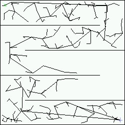
Then a greedier approach is introduced (the CONNECT function, shown in algorithms 3 and 4), which repeats EXTEND until an obstacle is reached. This ensures that most of the time we will be adding states to the tree, instead of just rejecting new random states. The second extension is the use of two trees, rooted at and , which are grown towards each other (see figure 2.1). This significantly decreases the time needed to find a path.
2.2 Retraction-Based RRT Planner
The Retraction-based RRT Planner presented in [ZM08] aims at improving the performance of the standard offline RRT in static environments with narrow passages. The basic idea of the function in algorithm 5 is to iteratively retract a randomly generated configuration that is in to the closest boundary point in . So, instead of using the standard extension that tries to extend in a straight line from to , it extends from to the closest point in to . This gives more samples in narrow passages. This technique could easily be applied to on-line RRT planners.
2.3 Execution Extended RRT
The Execution Extended RRT presented in [BV02] introduces two extensions to RRT to build an on-line planner, the waypoint cache and adaptive cost penalty search, which improve re-planning efficiency and the quality of generated paths. ERRT uses a kd-tree (see section 2.7) to speed nearest neighbor look-up, and does not use bidirectional search. The waypoint cache is implemented by keeping a constant size array of states, and whenever a plan is found, all the states in the plan are placed in the cache with random replacement. Then, when the tree is no longer valid, a new tree must be grown, and there are three possibilities for choosing a new target state, as shown in algorithm 6, which is used instead of in previous algorithms. With probability P[goal], the goal is chosen as the target; with probability P[waypoint], a random waypoint is chosen, and with the remaining probability a uniform state is chosen as before. In [BV02] the values used are P[goal] and P[waypoint].
Another extension is adaptive cost penalty search, where the planner adaptively modified a parameter to help it find shorter paths. A value of 1 for beta will always extend from the root node, while a value of 0 is equivalent to the original algorithm. However, the paper [BV02] lacks implementation details and experimental results on this extension.
2.4 Dynamic RRT
The Dynamic Rapidly-Exploring Random Tree described in [FKS06] is a probabilistic analog to the widely used D* family of algorithms. It works by growing a tree from to , as shown in algorithm 7. This has the advantage that the root of the tree does not have to be moved during the lifetime of the planning and execution. In some problem classes the robot has limited range sensors, thus moving or newly appearing obstacles will be near the robot, not near the goal. In general this strategy attempts to trim smaller branches that are farther away from the root. When new information concerning the configuration space is received, the algorithm removes the newly-invalid branches of the tree (algorithms 9 and 10), and grows the remaining tree, focusing, with a certain probability (empirically tuned to in [FKS06]) to a vicinity of the recently trimmed branches, by using the waypoint cache of the ERRT (algorithm 6). In experiments presented in [FKS06] DRRT vastly outperforms ERRT.
2.5 Multipartite RRT
Multipartite RRT presented in [ZKB07] is another RRT variant which supports planning in unknown or dynamic environments. MP-RRT maintains a forest of disconnected sub-trees which lie in , but which are not connected to the root node of , the main tree. At the start of a given planning iteration, any nodes of and which are no longer valid are deleted, and any disconnected sub-trees which are created as a result are placed into (as seen in algorithms 11 and 12). With given probabilities, the algorithm tries to connect to a new random state, to the goal state, or to the root of a tree in (algorithm 13). In [ZKB07], a simple greedy smoothing heuristic is used, that tries to shorten paths by skipping intermediate nodes. The MP-RRT is compared to an iterated RRT, ERRT and DRRT, in 2D, 3D and 4D problems, with and without smoothing. For most of the experiments, MP-RRT modestly outperforms the other algorithms, but in the 4D case with smoothing, the performance gap in favor of MP-RRT is much larger. The authors explained this fact due to MP-RRT being able to construct much more robust plans in the face of dynamic obstacle motion. Another algorithm that utilizes the concept of forests is Reconfigurable Random Forests (RRF) presented in [LS02], but without the success of MP-RRT.
2.6 Rapidly Exploring Evolutionary Tree
The Rapidly Exploring Evolutionary Tree, introduced in [MWS07] uses a bidirectional RRT and a kd-tree (see section 2.7) for efficient nearest neighbor search. The modifications to the function are shown in algorithm 14. The re-balancing of a kd-tree is costly, and in this paper a simple threshold on the number of nodes added before re-balancing was used. The authors suggest using the method described in [AL02] and used in [BV02] to improve the search speed. The novelty in this algorithm comes from the introduction of an evolutionary algorithm [BFM97] that builds a population of biases for the RRTs. The genotype of the evolutionary algorithm consists of a single robot configuration for each tree. This configuration is sampled instead of the uniform distribution. To balance exploration and exploitation, the evolutionary algorithm was designed with 50% elitism. The fitness function is related to the number of left and right branches traversed during the insertion of a new node in the kd-tree. The goal is to introduce a bias to the RRT algorithm which shows preference to nodes created away from the center of the tree. The authors suggest combining RET with DRRT or MP-RRT.
2.7 Multidimensional Binary Search Trees
The kd-tree, first introduced in [Ben75], is a binary tree in which every node is a k-dimensional point. Every non-leaf node generates a splitting hyperplane that divides the space into two subspaces. In the RRT algorithm, the number of points grows incrementally, unbalancing the tree, thus slowing nearest-neighbor queries. Re-balancing a kd-tree is costly, so in [AL02] the authors present another approach: A vector of trees is constructed, where for points there is a tree that contains points for each in the place of the binary representation of . As bits are cleared in the representation due to increasing , the trees are deleted, and the points are included in a tree that corresponds to the higher-order bit which is changed to . This general scheme incurs in logarithmic-time overhead, regardless of dimension. Experiments show a substantial performance increase compared to a naive brute-force approach.
2.8 Evolutionary Planner/Navigator
An evolutionary algorithm [BFM97] is a generic population-based meta-heuristic optimization algorithm. It is inspired in biological evolution, using methods such as individual selection, reproduction and mutation. The population is composed of candidate solutions and they are evaluated according to a fitness function.
The Evolutionary Planner/Navigator presented in [XMZ96], [XMZT97], and [TX97] is an evolutionary algorithm for path finding in dynamic environments. A high level description is shown in algorithm 15. A difference with RRT is that it can optimize the path according to any fitness function defined (length, smoothness, etc), without the need for a post-processing step. Experimental tests have shown it has good performance for sparse maps, but no so much for difficult maps with narrow passages or too crowded with obstacles. However, when a feasible path is found, it is very efficient at optimizing it and adapting to the dynamic obstacles.
Every individual in the population is a sequence of nodes, representing nodes in a path consisting of straight-line segments. Each node consists of an pair and a state variable with information about the feasibility of the point and the path segment connecting it to the next point. Individuals have variable length.
Since a path can be either feasible or unfeasible, two evaluation functions are used. For feasible paths (equation 2.1), the goal is to minimize distance traveled, maintain a smooth trajectory and satisfy a clearance requirement (the robot should not approach the obstacles too closely). For unfeasible paths, we use equation 2.2, taken from [Xia97], where is the number of intersections of a whole path with obstacles and is the average number of intersections per unfeasible segment.
| (2.1) |
| (2.2) |
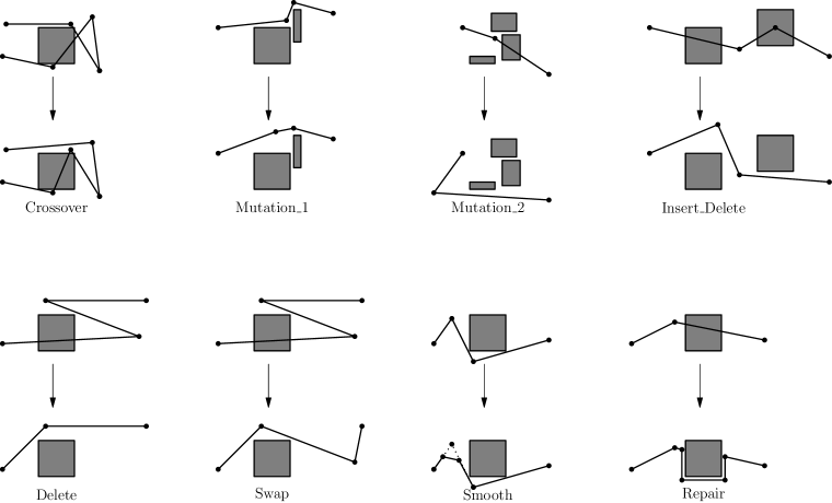
EP/N uses eight different operators, as shown in figure 2.2 (description taken from [XMZ96]):
-
Crossover: Recombines two (parent) paths into two new paths. The parent paths are divided randomly into two parts respectively and recombined: The first part of the first path with the second part of the second path, and the first part of the second path with the second part of the first path. Note that there can be different numbers of nodes in the two parent paths.
-
Mutate_1: Used to fine tune node coordinates in a feasible path for shape adjustment. This operator randomly adjusts node coordinates within some local clearance of the path so that the path remains feasible afterwards.
-
Mutate_2: Used for large random changes of node coordinates in a path, which can be either feasible or unfeasible.
-
Insert-Delete: Operates on an unfeasible path by inserting randomly generated new nodes into unfeasible path segments and deleting unfeasible nodes (i.e., path nodes that are inside obstacles).
-
Delete: Deletes nodes from a path, which can be either feasible or unfeasible. If the path is unfeasible, the deletion is done randomly. Otherwise, the operator decides whether a node should definitely be deleted based on some heuristic knowledge, and if a node is not definitely deletable, its deletion will be random.
-
Swap: Swaps the coordinates of randomly selected adjacent nodes in a path, which can be either feasible or unfeasible.
-
Smooth: Smoothens turns of a feasible path by “cutting corners,” i.e., for a selected node, the operator inserts two new nodes on the two path segments connected to that node respectively and deletes that selected node. The nodes with sharper turns are more likely to be selected.
-
Repair: Repairs a randomly selected unfeasible segment in a path by “pulling” the segment around its intersecting obstacle.
The probabilities of using each operator is set randomly at the beginning, and then are updated according to the success ratio of each operator, so more successful operators are used more often, and automatically chosen according to the instance of the problem, eliminating the difficult problem of hand tuning the probabilities.
In [TX97], the authors include a memory buffer for each individual to store good paths from its ancestors, which gave a small performance gain.
In [EAA04], the authors propose strategies for improving the stability and controlling population diversity for a simplified version of the EP/N. An improvement proposed by the authors in [XMZT97] is using heuristics for the initial population, instead of random initialization. We will consider this improvement in section 3.1.
Chapter 3 Proposed Techniques
3.1 Combining RRT and EP/N
As mentioned in section 2, RRT variants produce suboptimal solutions, which must later be post-processed for shortening, smoothing or other desired characteristics. On the other hand, EP/N, presented in section 2.8, can optimize a solution according to any given fitness function. However, this algorithm is slower at finding a first feasible solution. In this section we propose a combined approach, that uses RRT to find an initial solution to be used as starting point for EP/N, taking advantage of the strong points of both algorithms.
3.1.1 The Combined Strategy
Initial Solution
EP/N as presented in section 2.8 can not find feasible paths in a reasonable amount of time in any but very sparse maps. For this reason, RRT will be used to generate a first initial solution, ignoring the effects produced by dynamic objects. This solution will be in the initial population of the evolutionary algorithm, along with random solutions.
Feasibility and Optimization
EP/N is the responsible of regaining feasibility when it is lost due to a moving obstacle or a new obstacle found in a partially known or totally unknown environment. If a feasible solution can not be found in a given amount of time, the algorithm is restarted, keeping its old population, but adding a new individual generated by RRT.
3.1.2 Algorithm Implementation
The combined RRT-EP/N algorithm proposed here works by alternating environment updates and path planning, as can be seen in algorithm 16. The first stage of the path planning (see algorithm 17) is to find an initial path using a RRT technique, ignoring any cuts that might happen during environment updates. Thus, the RRT ensures that the path found does not collide with static obstacles, but might collide with dynamic obstacles in the future. When a first path is found, the navigation is done by using the standard EP/N as shown in algorithm 15.
3.2 A Simple Multi-stage Probabilistic Algorithm
In highly dynamic environments, with many (or a few but fast) relatively small moving obstacles, regrowing trees are pruned too fast, cutting away important parts of the trees before they can be replaced. This dramatically reduces the performance of the algorithms, making them unsuitable for these classes of problems. We believe that better performance could be obtained by slightly modifying a RRT solution using simple obstacle-avoidance operations on the new colliding points of the path by informed local search. The path could be greedily optimized if the path has reached the feasibility condition.
3.2.1 A Multi-stage Probabilistic Strategy
If solving equation 1.1 is not a simple task in static environments, solving dynamic versions turns out to be even more difficult. In dynamic path planning we cannot wait until reaching the optimal solution because we must deliver a “good enough” plan within some time restriction. Thus, a heuristic approach must be developed to tackle the on-line nature of the problem. The heuristic algorithms presented in sections 2.3, 2.4 and 2.5 extend a method developed for static environments, which produces poor response to highly dynamic environments and unwanted complexity of the algorithms.
We propose a multi-stage combination of simple heuristic and probabilistic techniques to solve each part of the problem: Feasibility, initial solution and optimization.
Feasibility
The key point in this problem is the hard constraint in equation 1.1 which must be met before even thinking about optimizing. The problem is that in highly dynamic environments a path turns rapidly from feasible to unfeasible — and the other way around — even if our path does not change. We propose a simple informed local search to obtain paths in . The idea is to randomly search for a path by modifying the nearest colliding segment of the path. As we include in the search some knowledge of the problem, the informed term is coined to distinguish it from blind local search. The details of the operators used for the modification of the path are described in section 3.2.2. If a feasible solution can not be found in a given amount of time, the algorithm is restarted, with a new starting point generated by a RRT variant.
Initial Solution
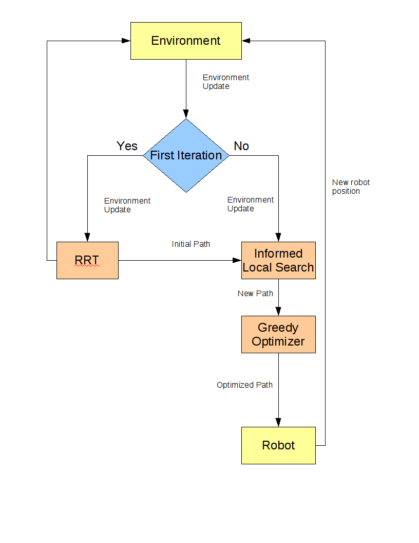
The problem with local search algorithms is that they repair a solution that it is assumed to be near the feasibility condition. Trying to produce feasible paths from scratch with local search (or even with evolutionary algorithms [XMZT97]) is not a good idea due the randomness of the initial solution. Therefore, we propose feeding the informed local search with a standard RRT solution at the start of the planning, as can be seen in figure 3.1.
Optimization
Without an optimization criterion, the path could grow infinitely large in time or size. Therefore, the function must be minimized when a (temporary) feasible path is obtained. A simple greedy technique is used here: We test each point in the solution to check if it can be removed maintaining feasibility; if so, we remove it and check the following point, continuing until reaching the last one.
3.2.2 Algorithm Implementation
The multi-stage algorithm proposed in this thesis works by alternating environment updates and path planning, as can be seen in algorithm 18. The first stage of the path planning (see algorithm 19) is to find an initial path using a RRT technique, ignoring any cuts that might happen during environment updates. Thus, RRT ensures that the path found does not collide with static obstacles, but might collide with dynamic obstacles in the future. When a first path is found, the navigation is done by alternating a simple informed local search and a simple greedy heuristic as shown in figure 3.1.
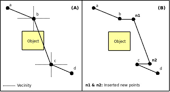
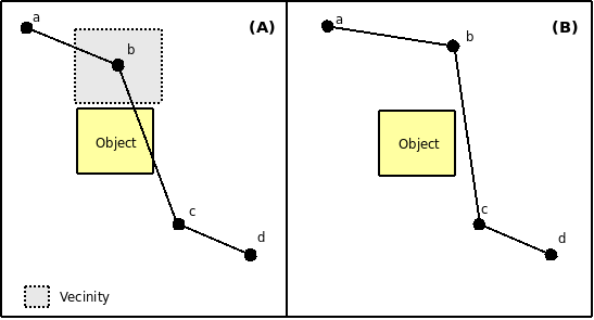
The second stage is the informed local search, which is a two step function composed by the arc and mutate operators (algorithms 20 and 21). The first one tries to build a square arc around an obstacle, by inserting two new points between two points in the path that form a segment colliding with an obstacle, as shown in figure 3.2. The second step in the function is a mutation operator that moves a point close to an obstacle to a random point in the vicinity, as explained graphically in figure 3.3. The mutation operator is inspired by the ones used in the Adaptive Evolutionary Planner/Navigator (EP/N) presented in [XMZT97], while the arc operator is derived from the arc operator in the Evolutionary Algorithm presented in [AR05].
The third and last stage is the greedy optimization heuristic, which can be seen as a post-processing for path shortening, that eliminates intermediate nodes if doing so does not create collisions, as is described in the algorithm 22.
Chapter 4 Experimental Setup and Results
4.1 Experimental Setup
Although the algorithms developed in this thesis are aimed at dynamic environments, for the sake of completeness they will also be compared in partially known environments and in totally unknown environments, where some or all of the obstacles become visible to the planner as the robot approaches each one of them, simulating a robot with limited sensor range.
4.1.1 Dynamic Environment
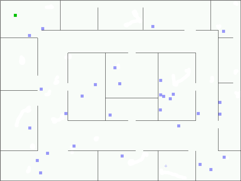
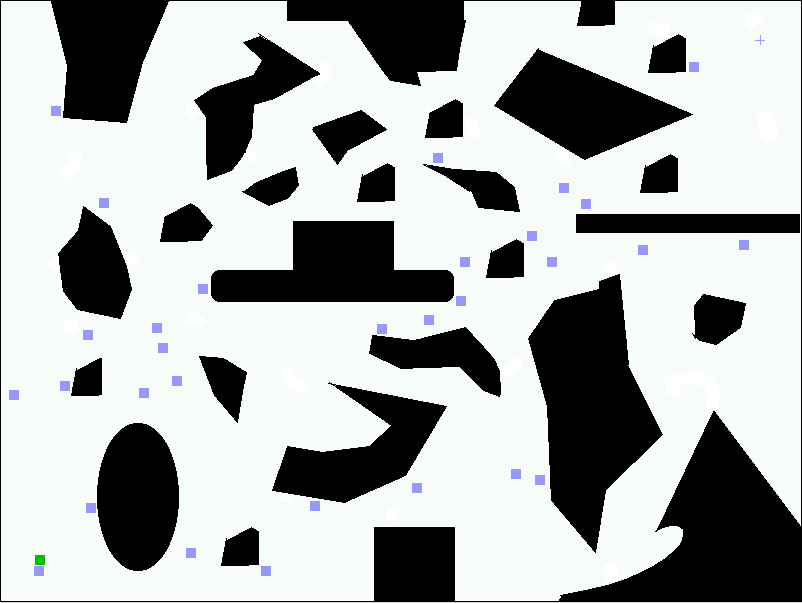
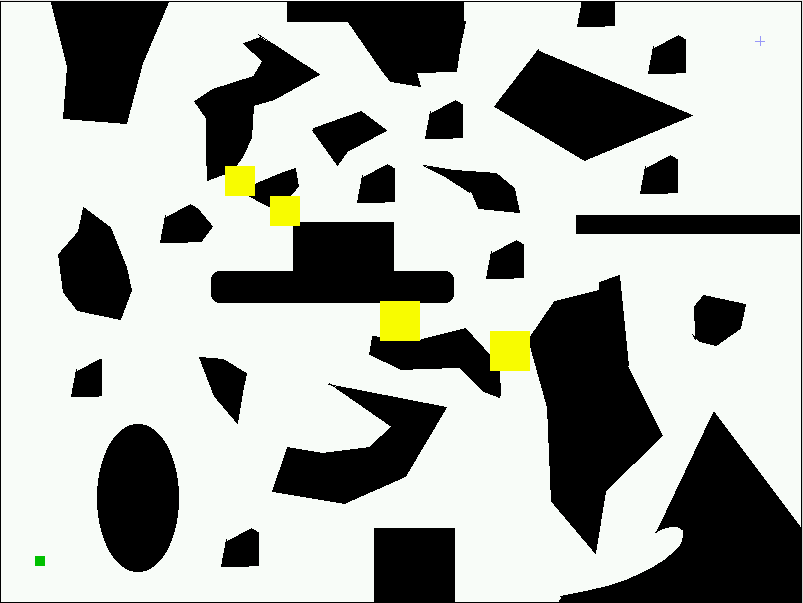
The first environment for our experiments consists on two maps with 30 moving obstacles the same size of the robot, with a random speed between 10% and 55% the speed of the robot. Good performance in this environment is the main focus of this thesis. This dynamic environments are illustrated in figures 4.1 and 4.2.
4.1.2 Partially Known Environment
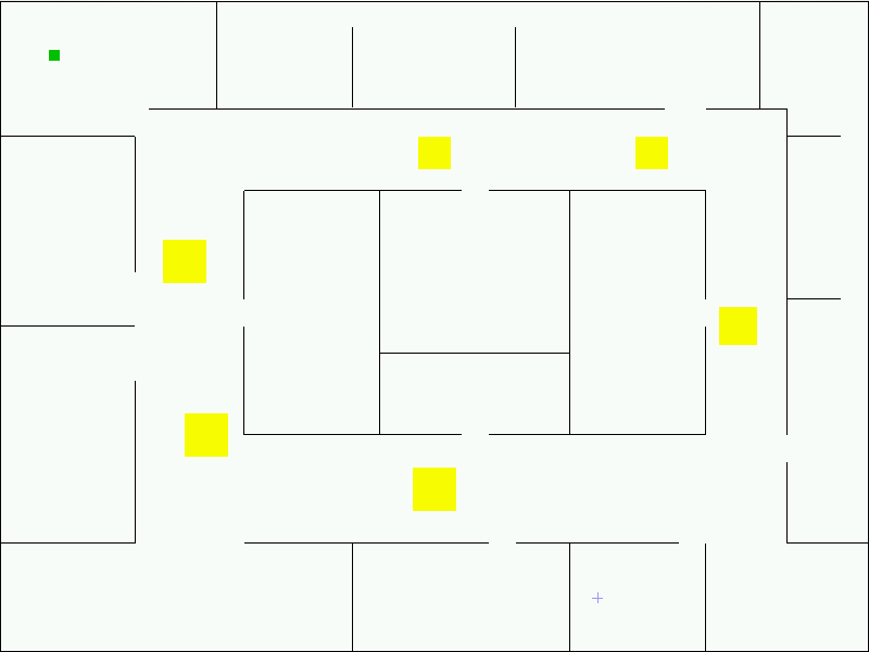
The second environment uses the same maps, but with a few obstacles, three to four times the size of the robot, that become visible when the robot approaches each one of them. This is the kind of environment that most dynamic RRT variants were designed for. The partially known environments are illustrated in figure 4.3 and 4.4.
4.1.3 Unknown Environment
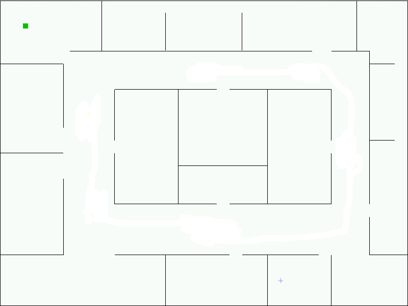
For completeness sake, we will compare the different technique in a third environment, were we use one of the maps presented before, but all the obstacles will initially be unknown to the planners, and will become visible as the robot approaches them, forcing several re-plans. This unknown environment is illustrated in figure 4.5.
4.2 Implementation Details
The algorithms where implemented in C++ using the MoPa framework111MoPa homepage: https://csrg.inf.utfsm.cl/twiki4/bin/view/CSRG/MoPa partly developed by the author. This framework features exact collision detection, three different map formats (including .pbm images from any graphic editor), dynamic, unknown and partially known environments and support for easily adding new planners. One of the biggest downsides is that it only supports rectangular objects, so several objects must be used to represent other geometrical shapes, as in figure 4.4, composed of 1588 rectangular objects.
There are several variations that can be found in the literature when implementing RRT. For all our RRT variants, the following are the details on where we departed from the basics:
-
1.
We always use two trees rooted at and .
-
2.
Our EXTEND function, if the point cannot be added without collisions to a tree, adds the mid point between the nearest tree node and the nearest collision point to it.
-
3.
In each iteration, we try to add the new randomly generated point to both trees, and if successful in both, the trees are merged, as proposed in [KL00].
-
4.
We believe that there might be significant performance differences between allowing or not allowing the robot to advance towards the node nearest to the goal when the trees are disconnected, as proposed in [ZKB07].
In point 4 above, the problem is that the robot would become stuck if it enters a small concave zone of the environment (like a room in a building) while there are moving obstacles inside that zone, but otherwise it can lead to better performance. Therefore we present results for both kinds of behavior: DRRT-adv and MP-RRT-adv move even when the trees are disconnected, while DRRT-noadv and MP-RRT-noadv only move when the trees are connected.
In MP-RRT, the forest was handled by simply replacing the oldest tree in it if the forest had reached the maximum allowed size.
Concerning the parameter selection, the probability for selecting a point in the vicinity of a point in the waypoint cache in DRRT was set to 0.4 as suggested in [FKS06]. The probability for trying to reuse a subtree in MP-RRT was set to 0.1 as suggested in [ZKB07]. Also, the forest size was set to 25 and the minimum size of a tree to be saved in the forest was set to 5 nodes.
For the combined RRT-EP/N, it was considered the planner was stuck after two seconds without a feasible solution in the population, at which point a new solution from a RRT variant is inserted into the population. For the simple multi-stage probabilistic algorithm, the restart is made after one second of encountering the same obstacle along the planned path. This second approach, which seems better, cannot be applied to the RRT-EP/N, because there is no single path to check for collisions, but instead a population of paths. The restart times where manually tuned.
4.3 Results
The three algorithms were run a hundred times in each environment and map combination. The cutoff time was five minutes for all tests, after which the robot was considered not to have reached the goal. Results are presented concerning:
-
•
Success rate (S.R.): The percentage of times the robot arrived at the goal, before reaching the five minutes cutoff time. This does not account for collisions or time the robot was stopped waiting for a plan.
-
•
Number of nearest neighbor lookups performed by each algorithm (N.N.): One of the possible bottlenecks for tree-based algorithms
-
•
Number of collision checks performed (C.C.), which in our specific implementation takes a significant percentage of the running time
-
•
Time it took the robot to reach the goal, the standard deviation.
4.3.1 Dynamic Environment Results
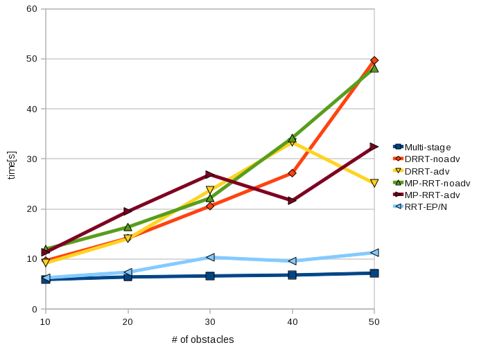
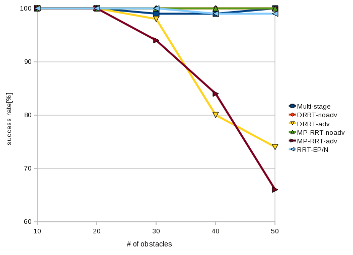
The results in tables 4.1 and 4.2 show that the multi-stage algorithm takes considerably less time than the DRRT and MP-RRT to reach the goal, with far less collision checks. The combined RRT-EP/N is a close second. It was expected that nearest neighbor lookups would be much lower in both combined algorithms than in the RRT variants, because they are only performed in the initial phase and restarts, not during navigation. The combined algorithms produce more consistent results within a map, as shown by their smaller standard deviations, but also across different maps. An interesting fact is that in map 1 DRRT is slightly faster than MP-RRT, and in map 2 MP-RRT is faster than DRRT. However the differences are too small to draw any conclusions. Figures 4.6 and 4.7 show the times and success rates of the different algorithms, when changing the number of dynamic obstacles in map 1. The simple multi-stage algorithm and the mixed RRT-EP/N clearly show the best performance, while the DRRT-adv and MP-RRT-adv significantly reduce their success rate when confronted to more than 30 moving obstacles.
| Algorithm | S.R.[%] | C.C. | N.N. | Time[s] | |
|---|---|---|---|---|---|
| Multi-stage | 99 | 23502 | 1122 | 6.62 | 0.7 |
| RRT-EP/N | 100 | 58870 | 1971 | 10.34 | 14.15 |
| DRRT-noadv | 100 | 91644 | 4609 | 20.57 | 20.91 |
| DRRT-adv | 98 | 107225 | 5961 | 23.72 | 34.33 |
| MP-RRT-noadv | 100 | 97228 | 4563 | 22.18 | 14.71 |
| MP-RRT-adv | 94 | 118799 | 6223 | 26.86 | 41.78 |
| Algorithm | S.R.[%] | C.C. | N.N. | Time[s] | |
|---|---|---|---|---|---|
| Multi-stage | 100 | 10318 | 563 | 8.05 | 1.47 |
| RRT-EP/N | 100 | 21785 | 1849 | 12.69 | 5.75 |
| DRRT-noadv | 99 | 134091 | 4134 | 69.32 | 49.47 |
| DRRT-adv | 100 | 34051 | 2090 | 18.94 | 17.64 |
| MP-RRT-noadv | 100 | 122964 | 4811 | 67.26 | 42.45 |
| MP-RRT-adv | 100 | 25837 | 2138 | 16.34 | 13.92 |
4.3.2 Partially Known Environment Results
Taking both maps into consideration, the results in tables 4.3 and 4.4 show that both combined algorithms are faster and more consistent than the RRT variants, with the simple multi-stage algorithm being faster in both. These results were unexpected, as the combined algorithms were designed for dynamic environments. It is worth to notice though, that in map 1 DRRT-adv is a close second, but in map 2 it is a close last, so its lack of reliability does not make it a good choice in this scenario. In this environment, as in the dynamic environment, in map 1 DRRT is faster than MP-RRT, while the opposite happens in map 2.
| Algorithm | S.R.[%] | C.C. | N.N. | Time[s] | |
|---|---|---|---|---|---|
| Multi-stage | 100 | 12204 | 1225 | 7.96 | 2.93 |
| RRT-EP/N | 99 | 99076 | 1425 | 9.95 | 2.03 |
| DRRT-noadv | 100 | 37618 | 1212 | 11.66 | 15.39 |
| DRRT-adv | 99 | 12131 | 967 | 8.26 | 2.5 |
| MP-RRT-noadv | 99 | 49156 | 1336 | 13.82 | 17.96 |
| MP-RRT-adv | 97 | 26565 | 1117 | 11.12 | 14.55 |
| Algorithm | S.R.[%] | C.C. | N.N. | Time[s] | |
|---|---|---|---|---|---|
| Multi-stage | 100 | 12388 | 1613 | 17.66 | 4.91 |
| RRT-EP/N | 100 | 42845 | 1632 | 22.01 | 6.65 |
| DRRT-noadv | 99 | 54159 | 1281 | 32.67 | 15.25 |
| DRRT-adv | 100 | 53180 | 1612 | 32.54 | 19.81 |
| MP-RRT-noadv | 100 | 48289 | 1607 | 30.64 | 13.97 |
| MP-RRT-adv | 100 | 38901 | 1704 | 25.71 | 12.56 |
4.3.3 Unknown Environment Results
Results in table 4.5 present the combined RRT-EP/N clearly as the faster algorithm in unknown environments, with the multi-stage algorithm in second place. In contrast to dynamic and partially known environments in this same map, MP-RRT is faster than DRRT.
| Algorithm | S.R.[%] | C.C. | N.N. | Time[s] | |
|---|---|---|---|---|---|
| Multi-stage | 100 | 114987 | 2960 | 13.97 | 3.94 |
| RRT-EP/N | 100 | 260688 | 2213 | 10.69 | 2.08 |
| DRRT-noadv | 98 | 89743 | 1943 | 18.38 | 22.01 |
| DRRT-adv | 100 | 104601 | 2161 | 19.64 | 34.87 |
| MP-RRT-noadv | 99 | 129785 | 1906 | 21.82 | 27.23 |
| MP-RRT-adv | 100 | 52426 | 1760 | 16.05 | 10.87 |
Chapter 5 Conclusions and Future Work
The new multi-stage algorithm proposed here has good performance in very dynamic environments. It behaves particularly well when several small obstacles are moving around at random. This is explained by the fact that if the obstacles are constantly moving, they will sometimes move out of the way by themselves, which our algorithm takes advantage of, while RRT based ones do not, they just drop branches of the tree that could prove useful again just a few moments later. The combined RRT-EP/N, although having more operators, and automatic adjustment of the operator probabilities according to their effectiveness, is still better than the RRT variants, but about 55% slower than the simple multi-stage algorithm. This is explained by the number of collision checks performed, more than twice than the multi-stage algorithm, because collision checks must be performed for the entire population, not just a single path.
In the partially known environment, even though the difference in collision checks is even greater than in dynamic environments, the RRT-EP/N performance is about 25% worse than the multi-stage algorithm. Overall, the RRT variants are closer to the performance of both combined algorithms.
In the totally unknown environment, the combined RRT-EP/N is about 30% faster than the simple multi-stage algorithm, and both outperform the RRT variants, with much smaller times and standard deviations.
All things considered, the simple multi-stage algorithm is the best choice in most situations, with faster and more predictable planning times, a higher success rate, fewer collision checks performed and, above all, a much simpler implementation than all the other algorithms compared.
This thesis shows that a multi-stage approach, using different techniques for initial plannning and navigation, outperforms current probabilistic sampling techniques in dynamic, partially known and unknown environments.
Part of the results presented in this thesis are published in [BALS09].
5.1 Future Work
We propose several areas of improvement for the work presented in this thesis.
5.1.1 Algorithms
The most promising area of improvement seems to be to experiment with different on-line planners such as a version of the EvP ([AR05] and [AR08]) modified to work in continuous configuration space or a potential field navigator. Also, the local search presented here could benefit from the use of more sophisticated operators and the parameters for the RRT variants (such as forest size for MP-RRT), and the EP/N (such as population size) could benefit from being tuned specifically for this implementation, and not simply reusing the parameters found in previous work.
Another area of research that could be tackled is extending this algorithm to higher dimensional problems, as RRT variants are known to work well in higher dimensions.
Finally, as RRT variants are suitable for kinodynamic planning, we only need to adapt the on-line stage of the algorithm to have a new multi-stage planner for problems with kinodynamic constraints.
5.1.2 Framework
The MoPa framework could benefit from the integration of a third party logic layer, with support for arbitrary geometrical shapes, a spatial scene graph and hierarchical maps. Some candidates would be OgreODE [Ogr], Spring RTS [Spr] and ORTS [ORT].
Other possible improvements are adding support for other map formats, including discrimination of static and moving obstacles, limited sensor range simulation and integration with external hardware such as the Lego NXT [Leg], to run experiments in a more realistic scenario.
Bibliography
- [AL02] A. Atramentov and S.M. LaValle. Efficient nearest neighbor searching for motion planning. In Proceedings of the IEEE International Conference on Robotics and Automation, volume 1, pages 632–637 vol.1, 2002.
- [Alf05] T. Alfaro. Un algoritmo evolutivo para la resolución del problema de planificación de rutas de un robot móvil. Master’s thesis, Departamento de Informática, Universidad Técnica Federico Santa María, June 2005.
- [AR05] T. Alfaro and M. Riff. An on-the-fly evolutionary algorithm for robot motion planning. Lecture Notes in Computer Science, 3637:119, 2005.
- [AR08] T. Alfaro and M. Riff. An evolutionary navigator for autonomous agents on unknown large-scale environments. Intelligent Automation and Soft Computing, 14(1):105, 2008.
- [BALS09] N.A. Barriga, M. Araya-Lopez, and M. Solar. Combining a probabilistic sampling technique and simple heuristics to solve the dynamic path planning problem. In Proceedings XXVIII International Conference of the Chilean Computing Science Society (SCCC), 2009.
- [Ben75] J.L. Bentley. Multidimensional binary search trees used for associative searching. Communications of the ACM, 18(9):517, 1975.
- [BFM97] T. Bäck, DB Fogel, and Z. Michalewicz. Handbook of Evolutionary Computation. Taylor & Francis, 1997.
- [BV02] J. Bruce and M. Veloso. Real-time randomized path planning for robot navigation. In Proceedings of the IEEE/RSJ International Conference on Intelligent Robots and Systems, volume 3, pages 2383–2388 vol.3, 2002.
- [EAA04] A. Elshamli, HA Abdullah, and S. Areibi. Genetic algorithm for dynamic path planning. In Proceedings of the Canadian Conference on Electrical and Computer Engineering, volume 2, 2004.
- [FKS06] D. Ferguson, N. Kalra, and A. Stentz. Replanning with RRTs. In Proceedings of the IEEE International Conference on Robotics and Automation, pages 1243–1248, 15-19, 2006.
- [HA92] Yong K. Hwang and Narendra Ahuja. Gross motion planning — a survey. ACM Computing Surveys, 24(3):219–291, 1992.
- [KL00] Jr. Kuffner, J.J. and S.M. LaValle. RRT-connect: An efficient approach to single-query path planning. In Proceedings of the IEEE International Conference on Robotics and Automation, volume 2, pages 995–1001 vol.2, 2000.
- [KSLO96] L.E. Kavraki, P. Svestka, J.-C. Latombe, and M.H. Overmars. Probabilistic roadmaps for path planning in high-dimensional configuration spaces. IEEE Transactions on Robotics and Automation, 12(4):566–580, August 1996.
- [Lav98] S.M. Lavalle. Rapidly-Exploring Random Trees: A new tool for path planning. Technical report, Computer Science Department, Iowa State University, 1998.
- [Leg] Lego Mindstorms. http://mindstorms.lego.com/.
- [LKJ99] S.M. LaValle and J.J. Kuffner Jr. Randomized kinodynamic planning. In Proceedings of the IEEE International Conference on Robotics and Automation, volume 1, 1999.
- [LS02] Tsai-Yen Li and Yang-Chuan Shie. An incremental learning approach to motion planning with roadmap management. In Proceedings of the IEEE International Conference on Robotics and Automation, volume 4, pages 3411–3416 vol.4, 2002.
- [MWS07] S.R. Martin, S.E. Wright, and J.W. Sheppard. Offline and online evolutionary bi-directional RRT algorithms for efficient re-planning in dynamic environments. In Proceedings of the IEEE International Conference on Automation Science and Engineering, pages 1131–1136, September 2007.
- [NG04] G. Nagib and W. Gharieb. Path planning for a mobile robot using genetic algorithms. In Proceedings of the International Conference on Electrical, Electronic and Computer Engineering, pages 185–189, 2004.
- [NVTK03] I.K. Nikolos, K.P. Valavanis, N.C. Tsourveloudis, and A.N. Kostaras. Evolutionary algorithm based offline/online path planner for UAV navigation. IEEE Transactions on Systems, Man, and Cybernetics, Part B, 33(6):898–912, December 2003.
- [Ogr] OgreODE. http://www.ogre3d.org/wiki/index.php/OgreODE.
- [ORT] ORTS – A free software RTS game engine. http://www.cs.ualberta.ca/~mburo/orts/.
- [Spr] The Spring Project. http://springrts.com/.
- [Ste94] A. Stentz. Optimal and efficient path planning for partially-known environments. In Proceedings of the IEEE International Conference on Robotics and Automation, pages 3310–3317, 1994.
- [Ste95] A. Stentz. The focussed D* algorithm for real-time replanning. In International Joint Conference on Artificial Intelligence, volume 14, pages 1652–1659. LAWRENCE ERLBAUM ASSOCIATES LTD, 1995.
- [TX97] K.M. Trojanowski and Z.J. Xiao. Adding memory to the Evolutionary Planner/Navigator. In Proceedings of the IEEE International Conference on Evolutionary Computation, pages 483–487, 1997.
- [Xia97] J. Xiao. Handbook of Evolutionary Computation, chapter G3.6 The Evolutionary Planner/Navigator in a Mobile Robot Environment. IOP Publishing Ltd., Bristol, UK, UK, 1997.
- [XMZ96] J. Xiao, Z. Michalewicz, and L. Zhang. Evolutionary Planner/Navigator: Operator performance and self-tuning. In International Conference on Evolutionary Computation, pages 366–371, 1996.
- [XMZT97] J. Xiao, Z. Michalewicz, L. Zhang, and K. Trojanowski. Adaptive Evolutionary Planner/Navigator for mobile robots. Proceedings of the IEEE Transactions on Evolutionary Computation, 1(1):18–28, April 1997.
- [ZKB07] M. Zucker, J. Kuffner, and M. Branicky. Multipartite RRTs for rapid replanning in dynamic environments. In Proceedings of the IEEE International Conference on Robotics and Automation, pages 1603–1609, April 2007.
- [ZM08] Liangjun Zhang and D. Manocha. An efficient retraction-based RRT planner. In Proceedings of the IEEE International Conference on Robotics and Automation, pages 3743–3750, May 2008.