A Multi-stage Probabilistic Algorithm for Dynamic Path-Planning
Abstract
Probabilistic sampling methods have become very popular to solve single-shot path planning problems. Rapidly-exploring Random Trees (RRTs) in particular have been shown to be efficient in solving high dimensional problems. Even though several RRT variants have been proposed for dynamic replanning, these methods only perform well in environments with infrequent changes. This paper addresses the dynamic path planning problem by combining simple techniques in a multi-stage probabilistic algorithm. This algorithm uses RRTs for initial planning and informed local search for navigation. We show that this combination of simple techniques provides better responses to highly dynamic environments than the RRT extensions.
Index Terms:
artificial intelligence; motion planning; RRT; Multi-stage; local search; greedy heuristics;I Introduction
The dynamic path-planning problem consists in finding a suitable plan for each new configuration of the environment by recomputing a free-collision path using the new information available at each time step [5]. This kind of problem can be found for example by a robot trying to navigate through an area crowded with people, such as a shopping mall or supermarket. The problem has been addressed widely in its several flavors, such as cellular decomposition of the configuration space [12], partial environmental knowledge [11], high-dimensional configuration spaces [6] or planning with non-holonomic constraints [8]. However, simpler variations of this problem are complex enough that cannot be solved with deterministic techniques, and therefore they are worthy to study.
This paper is focused on finding and traversing a collision-free path in two dimensional space, for a holonomic robot 111A holonomic robot is a robot in which the controllable degrees of freedom is equal to the total degrees of freedom., without kinodynamic restrictions 222Kinodynamic planning is a problem in which velocity and acceleration bounds must be satisfied, in two different scenarios:
-
•
several unpredictably moving obstacles or adversaries.
-
•
partially known environment, when at some point in time, a new obstacle is found.
Besides from one (or few) new obstacle(s) in the second scenario we assume that we have perfect information of the environment at all times.
We will focus on continuous space algorithms and won’t consider algorithms that use discretized representations of the configuration space, such as D* [12], because for high dimensional problems, the configuration space becomes intractable in terms of both memory and computation time, and there is the extra difficulty of calculating the discretization size, trading off accuracy versus computational cost.
The offline RRT is efficient at finding solutions but they are far from being optimal, and must be post-processed for shortening, smoothing or other qualities that might be desirable in each particular problem. Furthermore, replanning RRTs are costly in terms of computation time, as well as evolutionary and cell-decomposition approaches. Therefore, the novelty of this work is the mixture of the feasibility benefits of the RRTs, the repairing capabilities of local search, and the computational inexpensiveness of greedy algorithms, into our lightweight multi-stage algorithm.
In the following sections, we present several path planning methods that can be applied to the problem described above. In section II-A we review the basic offline, single-query RRT, a probabilistic method that builds a tree along the free configuration space until it reaches the goal state. Afterwards, we introduce the most popular replanning variants of the RRT: ERRT in section II-B, DRRT in section II-C and MP-RRT in section II-D. Then, in section III we present our new hybrid multi-stage algorithm with the experimental results and comparisons in section IV. At last, the conclusions and further work are discussed in section V.
II Previous and Related Work
II-A Rapidly-Exploring Random Tree
One of the most successful probabilistic sampling methods for offline path planning
currently in use, is the Rapidly-exploring Random Tree (RRT), a single-query planner for
static environments, first introduced in
[9]. RRTs work towards finding a continuous path from a state
to a state in the free configuration space , by
building a tree rooted at . A new state is uniformly
sampled at random from the configuration space . Then the nearest node,
, in
the tree is located, and if and the shortest path from to
are in , then is added to the tree.
The tree
growth is stopped when a node is found near . To speed up convergence,
the search is usually biased to with a small probability.
In [7], two new features are added to RRTs. First, the EXTEND
function is introduced, which, instead of trying
to add directly to
the tree, makes a motion towards and tests for collisions.
Then a greedier approach is introduced, which repeats EXTEND until an obstacle is reached. This ensures that most of the time, we will be adding states to the tree, instead of just rejecting new random states. The second extension is the use of two trees, rooted at and , which are grown towards each other. This significantly decreases the time needed to find a path.
II-B ERRT
The execution extended RRT presented in [3] introduces two
RRTs extensions to build an on-line planner: the waypoint cache and
the adaptive cost penalty search, which improves re-planning efficiency
and the quality of generated paths.
The waypoint cache is implemented by keeping a constant
size array of states, and whenever a plan is found, all the states in the plan
are placed in the cache with random replacement. Then, when the tree is no
longer valid, a new tree must be grown, and there are three
possibilities for choosing a new target state. With probability
P[goal], the goal is chosen as the target; With probability
P[waypoint], a random waypoint is chosen, and with remaining
probability a uniform state is chosen as before. Values used in [3]
are P[goal] and P[waypoint].
In the other extension — the adaptive cost penalty search — the planner dynamically
modifies a parameter to help it finding shorter paths. A value of for will
always extend from the root node, while a value of is equivalent to the
original algorithm.
Unfortunately, the solution presented in [3] lacks of
implementation details and experimental results on this extension.
II-C Dynamic RRT
The Dynamic Rapidly-exploring Random Tree (DRRT) described in [4] is a probabilistic analog to the widely used D* family of algorithms. It works by growing a tree from to . The principal advantage is that the root of the tree does not have to be changed during the lifetime of the planning and execution. Also, in some problem classes the robot has limited range sensors, thus moving obstacles (or new ones) are typically near the robot and not near the goal. In general, this strategy attempts to trim smaller branches and farther away from the root. When new information concerning the configuration space is received, the algorithm removes the newly-invalid branches of the tree, and grows the remaining tree, focusing, with a certain probability(empirically tuned to in [4]) to a vicinity of the recently trimmed branches, by using the a similar structure to the waypoint cache of the ERRT. In experimental results DRRT vastly outperforms ERRT.
II-D MP-RRT
The Multipartite RRT presented in [14] is another RRT variant which supports planning in unknown or dynamic environments. The MP-RRT maintains a forest of disconnected sub-trees which lie in , but which are not connected to the root node of , the main tree. At the start of a given planning iteration, any nodes of and which are no longer valid are deleted, and any disconnected sub-trees which are created as a result are placed into . With given probabilities, the algorithm tries to connect to a new random state, to the goal state, or to the root of a tree in . In [14], a simple greedy smoothing heuristic is used, that tries to shorten paths by skipping intermediate nodes. The MP-RRT is compared to an iterated RRT, ERRT and DRRT, in 2D, 3D and 4D problems, with and without smoothing. For most of the experiments, MP-RRT modestly outperforms the other algorithms, but in the 4D case with smoothing, the performance gap in favor of MP-RRT is much larger. The authors explained this fact due to MP-RRT being able to construct much more robust plans in the face of dynamic obstacle motion. Another algorithm that utilizes the concept of forests is the Reconfigurable Random Forests (RRF) presented in [10], but without the success of MP-RRT.
III A Multi-stage Probabilistic Algorithm
In highly dynamic environments, with many (or a few but fast) relatively small moving obstacles, regrowing trees are pruned too fast, cutting away important parts of the trees before they can be replaced. This reduce dramatically the performance of the algorithms, making them unsuitable for these class of problems. We believe that a better performance could be obtained by slightly modifying a RRT solution using simple obstacle-avoidance operations on the new colliding points of the path by informed local search. Then, the path could be greedily optimized if the path has reached the feasibility condition.
III-A Problem Formulation
At each time-step, the proposed problem could be defined as an optimization problem with satisfiability constraints. Therefore, given a path our objective is to minimize an evaluation function (i.e. distance, time, or path-points), with the constraint. Formally, let the path a sequence of points, where a -dimensional point (), the set of obstacles positions at time , and an evaluation function of the path depending on the object positions. Then, our ideal objective is to obtain the optimum path that minimize our function within a feasibility restriction in the form
| (1) |
where is a feasibility function that equals to iff the path is collision free for the obstacles . For simplicity, we use very naive and functions, but this could be extended easily to more complex evaluation and feasibility functions. The used function assumes that the robot is a punctual object (dimensionless) in the space, and therefore, if all segments of the path do not collide with any object , we say that the path is in . The function will be the points count of , assuming that similar paths with less points are shorter. This could be easily changed to the euclidean distance, time, smoothness, clearness or several other optimization criterions.
III-B A Multi-stage Probabilistic Strategy
If solving equation 1 is not a simple task in static environments, solving dynamic versions turns out to be even more difficult. In dynamic path planning we cannot wait until reaching the optimal solution because we must deliver a “good enough” plan within some time quantum. Then, a heuristic approach must be developed to tackle the on-line nature of the problem. The heuristic algorithms presented in sections II-B, II-C and II-D, extend a method developed for static environments, which produce a poor response to highly dynamic environments and an unwanted complexity of the algorithms.
We propose a multi-stage combination of three simple heuristic probabilistic techniques to solve each part of the problem: feasibility, initial solution and optimization.
III-B1 Feasibility
The key point in this problem is the hard constraint in equation 1 which must be met before even thinking about optimizing. The problem is that in highly dynamic environments a path turns rapidly from feasible to unfeasible — and the other way around — even if our path does not change. We propose a simple informed local search to obtain paths in . The idea is to randomly search for a path by modifying the nearest colliding segment of the path. As we include in the search some knowledge of the problem, the informed term is coined to distinguish it from blind local search. The details of the operators used for the modification of the path are described in section III-C.
III-B2 Initial Solution
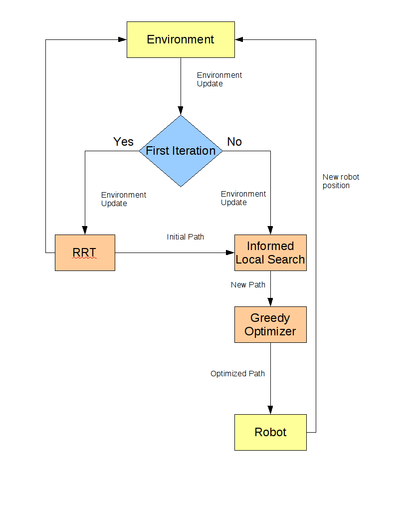
The problem with local search algorithms is that they repair a solution that it is assumed to be near the feasibility condition. Trying to produce feasible paths from scratch with local search (or even with evolutionary algorithms [13]) is not a good idea due the randomness of the initial solution. Therefore, we propose feeding the informed local search with a standard RRT solution at the start of the planning, as can be seen in figure 1.
III-B3 Optimization
Without an optimization criteria, the path could grow infinitely large in time or size. Therefore, the function must be minimized when a (temporary) feasible path is obtained. A simple greedy technique is used here: we test each point in the solution to check if it can be removed maintaining feasibility, if so, we remove it and check the following point, continuing until reaching the last one.
III-C Algorithm Implementation
The multi-stage algorithm proposed in this paper works by alternating environment updates and path planning, as can be seen in Algorithm 1. The first stage of the path planning (see Algorithm 2) is to find an initial path using a RRT technique, ignoring any cuts that might happen during environment updates. Thus, the RRT ensures that the path found does not collide with static obstacles, but might collide with dynamic obstacles in the future. When a first path is found, the navigation is done by alternating a simple informed local search and a simple greedy heuristic as is shown in Figure 1.
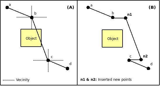
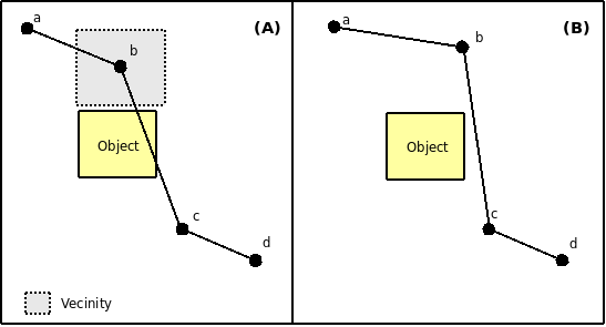
The second stage is the informed local search, which is a two step function composed by the arc and mutate operators (Algorithms 3 and 4). The first one tries to build a square arc around an obstacle, by inserting two new points between two points in the path that form a segment colliding with an obstacle, as is shown in Figure 2. The second step in the function is a mutation operator that moves a point close to an obstacle to a random point in the vicinity, as is graphically explained in Figure 3. The mutation operator is inspired by the ones used in the Adaptive Evolutionary Planner/Navigator(EP/N) presented in [13], while the arc operator is derived from the arc operator in the Evolutionary Algorithm presented in [1].
The third and last stage is the greedy optimization heuristic, which can be seen as a post-processing for path shortening, that eliminates intermediate nodes if doing so does not create collisions, as is described in the Algorithm 5.
IV Experiments and Results
The multi-stage strategy proposed here has been developed to navigate highly-dynamic environments, and therefore, our experiments should be aimed towards that purpose. Therefore, we have tested our algorithm in two highly-dynamic situations, both of them over a map representing an office building or shopping mall (i.e. with some static walls). Also, we have ran the DRRT and MP-RRT algorithms over the same situations in order to compare the performance of our proposal.
IV-A Experimental Setup
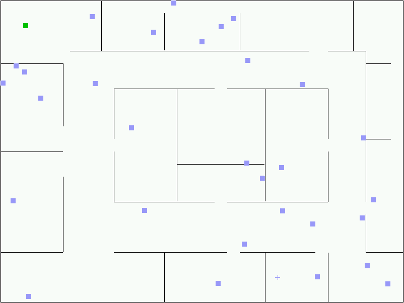
The first environment for our experiments consists on a map with 30 moving
obstacles the same size of the robot, with a random speed between 10% and 55%
the speed of the robot. This dynamic environment is shown in figure 4.
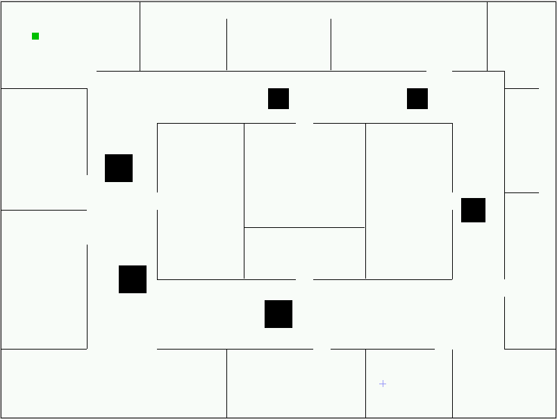
The second environment uses the same map, but with six obstacles, three to four
times the size of the robot, appearing at a predefined time and position. This
partially known environment is shown in figure 5.
The three algorithms were ran a hundred times in each environment. The cutoff time was five minutes for the first environment and one minute for the second, after which, the robot was considered not to have reached the goal.
IV-B Implementation Details
The algorithms where implemented in C++ using a framework
333MoPa homepage: https://csrg.inf.utfsm.cl/twiki4/bin/view/CSRG/MoPa
developed by the same authors.
There are several variations that can be found in the literature when implementing RRTs. For all our RRT variants, the following are the details on where we departed from the basics:
-
•
We always use two trees rooted at and .
-
•
Our EXTEND function, if the point cannot be added without collisions to a tree, adds the mid point between the nearest tree node and the nearest collision point to it.
-
•
In each iteration, we try to add the new randomly generated point to both trees, and if successful in both, the trees are merged, as proposed in [7].
-
•
We found that the success rate was somewhat lower if we allow the robot to advance towards the node nearest to the goal when the trees are disconnected, as proposed in [14]. The problem is that the robot would become stuck if it enters a small concave zone of the environment(like a room in a building) while there are moving obstacles inside that zone. Therefore our robot only moves when the trees are connected.
In MP-RRT, the forest was handled simply replacing the oldest tree in it if the forest had reached the maximum size allowed.
Concerning the parameter selection, the probability for selecting a point in the vicinity of a point in the waypoint cache in DRRT was set to 0.4 as suggested in [4]. The probability for trying to reuse a sub tree in MP-RRT was set to 0.1 as suggested in [14]. Also, the forest size was set to 25 and the minimum size of a tree to be saved in the forest was set to 5 nodes.
IV-C Dynamic Environment Results
The results in table I show that it takes our algorithm around a third of the time it takes the DRRT and MP-RRT to get to the goal, with far less collision checks. It was expected that nearest neighbor lookups would be much lower in the multi-stage algorithm than in the other two, because they are only performed in the RRT phase, not during navigation. However, the multi-stage algorithm seems to be slighty less dependable, as it arrived to the goal 98 out of 100 times, while the other two managed to arrive always.
| Algorithm | Success % | Coll. Checks | Nearest Neigh. | Time[s] |
|---|---|---|---|---|
| Multi-stage | 98 | 24364 | 1468 | 7.08 |
| DRRT | 100 | 92569 | 4536 | 19.81 |
| MP-RRT | 100 | 97517 | 4408 | 21.53 |
IV-D Partially Known Environment Results
The results in table II show that our multi-stage algorithm is very undependable, though faster than the other two when it actually reaches the goal. Due to the simplicity of our local search, and that it basically just avoids obstacles by stepping to the side or letting the obstacle move out of the way, when the changes to the environment are significant and obstacles do not move, it is very prone to getting stuck.
| Algorithm | Success % | Coll. Checks | Nearest Neigh. | Time[s] |
|---|---|---|---|---|
| Multi-stage | 44 | 4856 | 673 | 5.95 |
| DRRT | 100 | 9845 | 1037 | 7.25 |
| MP-RRT | 98 | 17029 | 1156 | 8.13 |
V Conclusions
The new multi-stage algorithm proposed here has a very good performance in very dynamic environments. It behaves particularly well when several small obstacles are moving around seemingly randomly. It’s major shortcoming is that it gets easily stuck when significant changes to the environment are made, such as big static obstacles appearing near the robot, a situation usually considered as a partially known environment.
V-A Future Work
There are several areas of improvement for the work presented in this paper. First of all, the multi-stage algorithm must recognize a situation where it is stuck, and restart an RRT from the current location, before continuing with the navigation phase. The detection could be as simple as recognizing that the robot has not moved out of a certain vicinity for a given period of time, or that the next collision in the planned path has been against the same obstacle during a given period of time, meaning that the local search has been unable to find a path around it. This will yield a much more dependable algorithm in different kinds of environments.
A second area of improvement is to experiment with different on-line planners such as the EP/N presented in [13], a version of the EvP([1] and [2]) modified to work in continuous configuration space or a potential field navigator. Also, the local search presented here, could benefit from the use of more sophisticated operators.
A third area of research that could be tackled is extending this algorithm to other types of environments, ranging from totally known and very dynamic, to static partially known or unknown environments. An extension to higher dimensional problems would be one logical way to go, as RRTs are know to work well in higher dimensions.
Finally, as RRTs are suitable for kinodynamic planning, we only need to adapt the on-line stage of the algorithm to have a new multi-stage planner for problem with kinodynamic constraints.
References
- [1] T. Alfaro and M. Riff. An On-the-fly Evolutionary Algorithm for Robot Motion Planning. Lecture Notes in Computer Science, 3637:119, 2005.
- [2] T. Alfaro and M. Riff. An Evolutionary Navigator for Autonomous Agents on Unknown Large-Scale Environments. INTELLIGENT AUTOMATION AND SOFT COMPUTING, 14(1):105, 2008.
- [3] J. Bruce and M. Veloso. Real-time randomized path planning for robot navigation. Intelligent Robots and System, 2002. IEEE/RSJ International Conference on, 3:2383–2388 vol.3, 2002.
- [4] D. Ferguson, N. Kalra, and A. Stentz. Replanning with rrts. Robotics and Automation, 2006. ICRA 2006. Proceedings 2006 IEEE International Conference on, pages 1243–1248, 15-19, 2006.
- [5] Y. K. Hwang and N. Ahuja. Gross motion planning—a survey. ACM Comput. Surv., 24(3):219–291, 1992.
- [6] L. Kavraki, P. Svestka, J.-C. Latombe, and M. Overmars. Probabilistic roadmaps for path planning in high-dimensional configuration spaces. Robotics and Automation, IEEE Transactions on, 12(4):566–580, Aug 1996.
- [7] J. Kuffner, J.J. and S. LaValle. Rrt-connect: An efficient approach to single-query path planning. Robotics and Automation, 2000. Proceedings. ICRA ’00. IEEE International Conference on, 2:995–1001 vol.2, 2000.
- [8] S. LaValle and J. Ku. Randomized kinodynamic planning, 1999.
- [9] S. M. Lavalle. Rapidly-exploring random trees: A new tool for path planning. Technical report, Computer Science Dept., Iowa State Univ., 1998.
- [10] T.-Y. Li and Y.-C. Shie. An incremental learning approach to motion planning with roadmap management. Robotics and Automation, 2002. Proceedings. ICRA ’02. IEEE International Conference on, 4:3411–3416 vol.4, 2002.
- [11] A. Stentz. Optimal and efficient path planning for partially-knownenvironments. In 1994 IEEE International Conference on Robotics and Automation, 1994. Proceedings., pages 3310–3317, 1994.
- [12] A. Stentz. The Focussed D^* Algorithm for Real-Time Replanning. In International Joint Conference on Artificial Intelligence, volume 14, pages 1652–1659. LAWRENCE ERLBAUM ASSOCIATES LTD, 1995.
- [13] J. Xiao, Z. Michalewicz, L. Zhang, and K. Trojanowski. Adaptive evolutionary planner/navigator for mobile robots. Evolutionary Computation, IEEE Transactions on, 1(1):18–28, Apr 1997.
- [14] M. Zucker, J. Kuffner, and M. Branicky. Multipartite rrts for rapid replanning in dynamic environments. Robotics and Automation, 2007 IEEE International Conference on, pages 1603–1609, April 2007.