The spike train statistics for consonant
and dissonant musical accords

Abstract

The simple system composed of three neural-like noisy elements is considered. Two of them (sensory neurons or sensors) are stimulated by noise and periodic signals with different ratio of frequencies, and the third one (interneuron) receives the output of these two sensors and noise. We propose the analytical approach to analysis of Interspike Intervals (ISI) statistics of the spike train generated by the interneuron. The ISI distributions of the sensory neurons are considered to be known. The frequencies of the input sinusoidal signals are in ratios, which are usual for music. We show that in the case of small integer ratios (musical consonance) the input pair of sinusoids results in the ISI distribution appropriate for more regular output spike train than in a case of large integer ratios (musical dissonance) of input frequencies. These effects are explained from the viewpoint of the proposed theory.

I Introduction

Since 1980-th it is well known that noise in physical systems doesn’t always play a negative role. The phenomena of coherence and stochastic resonance are found in different branches of science Gammaitoni et al. (1998), and the typical field of research regarding the constructive role of noise is a wide class of neural systems. Indeed, it is very difficult to forget about noise, investigating various parts of the central or the peripheral nervous system, even if a study is carried out in a framework of some mathematical model: noise is inherent for the dynamics of the membrane potential (due to ion channels’ noise) of neural fibers and somas; the synaptic junctions exhibit stochastic behavior; each neuron receives on the average $10^{4}$ inputs from its neighbors Gerstner and Kistler (2002) that in itself requires statistical methods of investigation, and etc. The motivating question of the given research is: how a signal survives in such noisy environment?

Looking for an approach to the problem we concentrated our attention to sensory systems Longtin et al. (2008); Fishman et al. (2001). Typically, in sensory systems there is a set of neurons (referred to as sensory neurons or sensors) receiving signals directly from the environment. For example, in a simple approximation of the mammals’ auditory system it is supposed that the basilar membrane performs the Fourier transformation on an input sound signal Helmholtz (1954), and the sensory neurons attached directly to this membrane, percept different sinusoidal components (depending on coordinates of connection along the membrane) of the sound as input. Under driving of these signals and the mentioned noise they generate trains of short impulses (spikes), which are transmitted to other neurons (interneurons) along neural fibers.

In a number of studies regarded to the neurodynamics under the noise influence the interspike intervals (ISI) statistics is of interest. In our model, composed of two sensors (stimulated by sinusoidal signals and noise) and one interneuron, we consider the ISI distribution (ISID) of each sensor to be known (from the previous works Burkitt (2006)) and investigate ISIDs of the output signal of the interneuron driven by a mixture of noise and the sensors’spike trains weighted by coupling coefficients. The system with the similar structure has been investigated in Ref. Balenzuela (2005); Lopera et al. (2006) for the purpose of Ghost Stochastic Resonance (GSR) phenomenon detection. The GSR term denotes existence of the maximum in the system response at some frequency, which is absent in the spectrum of the input signal. The maximum takes place at some optimal intensity of noise, which affects a system as well Chialvo et al. (2002).

Though we have not investigated this phenomenon in the presented work, our topic is closely connected with GSR studies due to high complexity (multimodality) of interneuron’s ISIDs comprising peaks inappropriate to input sinusoids’ periods or their multiples.

We show how the input signal composed of two sinusoids is transformed by the proposed noisy system into different types of spike trains, depending on the ratio of input frequencies. Looking for the differences in the statistical sense, we find out that the output ISIDs for some combinations of frequencies have sharp shapes similar to ISIDs of an interneuron driven by a well recognized (on a noise background) regular signal. Also, there is another type of the output ISID (for the other frequencies combinations), which has a blurred shape similar to an ISID of a neuron driven by randomly distributed impulses.

In fact, the difference between ”sharp” and ”blurred” shapes of ISIDs is more quantitative, than qualitative, but this difference indicates higher stability to noise of one combination of input sinusoids in comparison with another one. Investigation of this phenomenon can help to understand which types of input signals are able to survive in the noisy environment of the brain, which principles control this process, and what it means from the perceptional, cognitive, and other points of view.

On the other hand, in the real life a human deals with relatively simple combinations of sinusoidal signals, when listens to music. It is well known that musical accords (combinations of tones) are classified as consonant (pleasant, harmonious) or dissonant (unpleasant, disharmonious), depending on the ratio between frequencies Plomp and Levelt (1965). Thus, use of musical notations appears to be convenient in the context of our work for input signals classification purposes. However, we should emphasize that our results are obtained using the so-called ”just intonation” musical accords, i.e. frequencies of input sinusoids are related by ratios of whole numbers, that is not appropriate for modern music, but is more suitable in the presentation sense.

It is important also, that the consonance and the dissonance of accords are recognized by animals (which never deal with music) as well Fishman et al. (2001). So, the underlying principles seem to be common and fundamental for the auditory neural system of mammals. This is the good reason to use the neural-like model of the auditory apparatus as the object of research into effects related with simple signals (like simple musical accords) propagation through a noisy nonlinear environment.

It should be emphasized, that the ”noise benefits” phenomena like coherence resonance, stochastic resonance, ghost stochastic resonance, etc. are appropriate candidates for a solution of signal propagation and signal ”survival” problems. But they allow to reveal a very particular peculiarities of signal propagation through the nonlinear noisy environment of neural-like systems and don’t provide a full statistical picture. So, the main goal of the paper is to present an analytical description of principles, which control the statistics transformation process for spike trains propagated from one level of neurons to another one under the influence of noise.

In the paper we first describe the chosen model in details. After that we propose the analytical description applied to the interneuron’s ISI statistics. In order to prove the theoretical conclusions, we compare them with the results of computer simulations. Finally, we discuss an agreement of obtained results with the hypotheses of the consonance and the dissonance in music proposed by Helmholtz (1877) and Boomsliter&Creel (1961).

II Model

As a basis for the investigated neural-like system we have chosen the widely used model called Leaky Integrate-and-Fire (LIF) neuron. The input neurons (sensors) are driven by the external sinusoidal signals, and the output one (interneuron) receives the weighted spikes of the input neurons.

For simplicity we restrict consideration by a case of two sensors. As a result, the set of equations for our system can be written down in the following form:

$$\left\{\begin{array}[]{l}\dot{v}_{1}=-\mu_{1}v_{1}+A_{1}\cos\Omega_{1}t+\sqrt{D_{1}}\xi_{1}(t),\\ \dot{v}_{2}=-\mu_{2}v_{2}+A_{1}\cos\Omega_{2}t+\sqrt{D_{2}}\xi_{2}(t),\\ \dot{v}=-\mu v+k_{1}s_{1}(t)+k_{2}s_{2}(t)+\sqrt{D}\xi(t),\end{array}\right.$$ (1)

Here: $v_{i}(t)$ is the membrane potential of the $i^{th}$ sensory neuron; $\mu_{i}$ is the relaxation parameter; $A_{i}$ and $\Omega_{i}$ are the amplitude and the frequency of the corresponding harmonic input, respectively; $D_{i}$ is the sensor’s noise intensity; $\xi_{i}(t),(i=1,2)$ are the independent sources of the zero-mean $\delta$-correlated ($<\xi_{i}(t)\xi_{j}(t^{\prime})>=\delta(t-t^{\prime})\delta_{ij}$) white Gaussian noise (WGN) of the sensors; $v(t)$, $\mu$, $D$, and $\xi(t)$ are the membrane potential, relaxation parameter, noise intensity, and WGN of the output neuron (the third equation (1)), $<\xi(t)\xi(t^{\prime})>=\delta(t-t^{\prime})$, $<\xi(t)>=0$, and $<\xi(t)\xi_{i}(t^{\prime})>\equiv 0$.

The LIF neuron doesn’t comprise any mechanism of spike generation. So, as soon as the membrane potential of any neuron of the model reaches the threshold value $v_{th}$ we say that the spike is generated at the threshold crossing instant of time. The corresponding membrane potential is reset simultaneously to the initial value: $v_{i}^{0}$ for the sensors and $v^{0}$ for the interneuron.

The spike trains generated by the sensors and received by the interneuron are denoted as $s_{i}(t)=\sum\limits_{j=0}^{N_{i}(t)}\delta(t-t_{ij}),i=1,2$. Each spike train is weighted by the corresponding coupling coefficient $k_{i}$. Spikes are modelled by Dirac $\delta$-functions. The instants of time $t_{ij}$ correspond to threshold crossings by the sensors’ membrane potentials, $N_{i}(t)$ is the number of spikes generated by the $i^{th}$ sensor since the initial time. Obviously, the values $t_{ij}$ and their numbers $N_{i}(t)$ are directly related with amplitudes of input signals that means the system is nonlinear (by the definition of nonlinearity) even though it is not clear from the model Eq.(1).

All simulation and theoretical results presented in the paper are obtained using the following set of constant parameters: $\mu_{1}=\mu_{2}=1$, $\mu=0.3665$, $D_{1}=D_{2}=D=1.6\cdot 10^{-3}$, $k_{1}=k_{2}=0.98$, $v_{1}^{0}=v_{2}^{0}=0$, $v^{0}=-1$, and $v_{th}=1$, unless stated otherwise.

For the output neuron the refractory period ($T_{ref}$) is introduced explicitly: this neuron does not respond on any external signal after reset until the varying potential $v^{0}e^{-\mu(t-t_{res})}$ reaches the level $v=-0.1$. Hence, the refractory period can be written down in the following form:

$$T_{ref}=\frac{1}{\mu}\ln\left(-10v^{0}\right).$$

For the chosen parameters we have $T_{ref}=6.28$.

III Theoretical study

The first two equations of the system (1) are, obviously, independent differential equations, modelling the well-known Ornstein-Uhlenbeck process with the harmonic inhomogeneity and the reset rule. The statistics of interspike intervals in this case can be obtained analytically or numerically Burkitt (2006) and we consider it to be known.

The very important thing is that the spike trains of our sensors are non-Poisson ones. These spike trains are the input into the third neuron, and it means that the dynamics of the output neuron membrane potential is non-Markovian Cox (1967). Hence, we are compelled to investigate the ISI statistics of the output neuron using another analytical approach.

III.1 Solutions and presuppositions

It is possible to obtain analytical solutions for $v_{i}(t)$ and $v(t)$ Gardiner (1985):

$$\begin{array}[]{l}v_{i}(t)=\left[v_{i}(t_{0i})-\frac{A_{i}}{\sqrt{\Omega_{i}^{2}+1}}\cos(\Omega_{i}t_{0i}+\phi_{i})\right]\times\\ \times e^{-\mu_{i}(t-t_{0i})}+\frac{A_{i}}{\sqrt{\Omega_{i}^{2}+1}}\cos(\Omega_{i}t_{i}+\phi_{i})+\sqrt{D_{i}}\zeta_{i}(t),\\ \\ v(t)=v(t_{0})e^{-\mu(t-t_{0})}+\sum\limits_{i=1}^{2}k_{i}S_{i}(t)+\sqrt{D}\zeta(t).\end{array}$$ (2)

Here: $S_{i}(t)=\sum\limits_{j=0}^{N_{i}(t)}e^{-\mu(t-t_{ij})}$ is a sum of decaying impulses evoked by spikes of the $i^{th}$ sensory neuron; $\zeta_{i}(t)=\int\limits_{t_{0}}^{t}e^{-\mu_{i}(t-t^{\prime})}\xi_{i}(t^{\prime})dt^{\prime}$ is the colored Gaussian noise (Ornstein-Uhlenbeck process) with the variance
$\sigma^{2}_{i}(t)=\left<\zeta_{i}^{2}(t)\right>=\frac{1}{2\mu_{i}}\left(1-e^{-2\mu_{i}t}\right)$ and the probability distribution

$$w^{i}_{\zeta}(s)=\frac{1}{\sqrt{2\pi}\sigma_{i}(t)}\exp\left(-\frac{s^{2}}{2\sigma^{2}_{i}(t)}\right).$$

For the output neuron we have the same forms of $\zeta(t)$, $\sigma^{2}(t)$, and $w_{\zeta}(s)$. $t_{0i}$ and $t_{0}$ are the reset (spike generation) instants of time for the sensors or the interneuron, respectively; $\phi_{i}=\arctan\left(\frac{\Omega_{i}}{\mu_{i}}\right)$.

The temporal realizations of membrane potentials of neurons allow us to understand the conditions of spike generation by the output neuron and to establish connections between these events and input signals.

In order to perform the following analysis we utilize three main presuppositions:

1. The input harmonic signals are subthreshold to the sensors, i.e. the amplitude $A_{i}$ and the frequency $\Omega_{i}$ are in such a relation, that the signal $A_{i}\cos(\Omega_{i}t)$ is not able to evoke a spike of the $i^{th}$ sensor without noise ($D_{i}=0$). From the solutions (2) we obtain

   $$\frac{A_{i}}{\sqrt{\Omega_{i}^{2}+1}}<v_{th}.$$ (3)

2. Only one spike can be generated at each period of the harmonic driving force. But, at the same time, the spiking on each period is the most probable situation, and it means the relatively (to $\Omega_{i}$) high relaxation parameter $\mu_{i}$. Formally, the condition can be written down as:

   $$\frac{1}{\mu_{i}}\lesssim\frac{2\pi}{\Omega_{i}}.$$

3. Each of coupling coefficients $k_{i}$ is less than the threshold membrane potential value $v_{th}$. It means that any separate incoming spike evokes also a subthreshold impulse of the output neuron’s membrane potential $v(t)$, i.e. spike generation is impossible without noise. At the same time, the sum of two coefficients is greater than $v_{th}$:

   $$\left\{\begin{array}[]{l}k_{1,2}<v_{th},\\ k_{1}+k_{2}>v_{th}.\end{array}\right.$$

III.2 Probability distribution for the output neuron spike

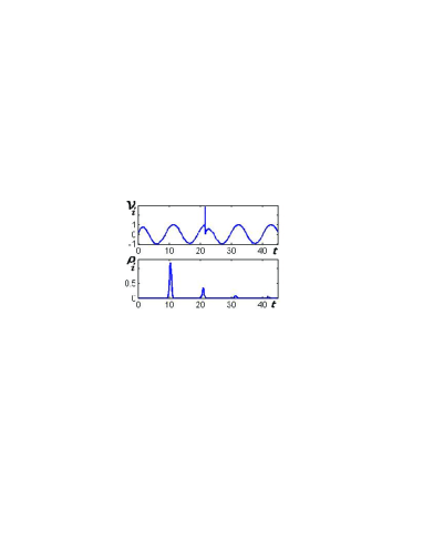
Let’s make some theoretical estimations. Initially all three neurons of the system Eq. (1) are reset, i.e. $v_{1}(0)=v_{1}^{0}$, $v_{2}(0)=v_{2}^{0}$, and $v(0)=v^{0}$. Since the starting time is $t=0$, we measure the first interspike period of the output neuron as the first passage time. The first passage time probability distributions (FPTPD) are considered to be known for the input neurons: $\rho_{1}(t)$ and $\rho_{2}(t)$, respectively. It means once time is started, we know necessary characteristics of a spikes sequence, coming from the $1^{st}$ and the $2^{nd}$ neurons to the $3^{rd}$ (output) one. Spikes of the sensory neurons have a highest probability to appear first time at maxima of harmonic driving force $(A_{i}/\sqrt{\Omega_{i}^{2}+1})\cos(\Omega_{i}t_{i}+\phi_{i})$. They have a narrow probability distribution near each of these maxima, and the probability of skipping one, two, etc. periods decays exponentially (see the Fig. 1).

Figure 1: The typical membrane potential realization $v_{i}(t)$ and the ISI distribution of the sensory neuron ($\Omega_{i}=0.6$, $A_{i}=1.165$). The highest probability of a spike after $t=0$ is near one period of external force ($t=10$). The probability of firing after two, three, etc. periods decreases rapidly.

So, we may analyze a probability $dP_{3}(t)$ to find the $3^{rd}$ neuron spike inside the short time interval $[t,t+dt]$.

For the chosen parameters there are only 4 probable situations in which the output (the $3^{rd}$ one) neuron generates a spike:

1. upon receiving a separate spike of the $1^{st}$ neuron;

2. upon receiving a separate spike of the $2^{nd}$ neuron;

3. upon receiving a $1^{st}$ neuron’s spike on a background of a $2^{nd}$’s one;

4. upon receiving a $2^{nd}$ neuron’s spike on a background of a $1^{st}$’s one.

The ”separate” spike means that at the time of its incoming the $3^{rd}$ neuron’s membrane potential $v(t)$ is driven only by noise, i.e. any previous perturbation over the noise level is relaxed.

The ”background” of some incoming spike means that this spike was not able to make fire the interneuron, but perturbed its membrane potential. This background decays exponentially with the decrement $\mu$ until it becomes hidden by noise.

Four described situations exclude each other, so, we may take them as independent probabilistic hypotheses. The probability of each hypothesis realization is directly connected with probabilities of the $1^{st}$ and $2^{nd}$ neurons’ spikes generation on the same time interval $[t,t+dt]$, and before it.

The probability of the $3^{rd}$ neuron spike generation in each of these 4 cases depends on the coupling coefficients $k_{1,2}$, the noise intensity $D$ and the membrane threshold $v_{th}$.

Hence, we obtain the first term of the contribution into the probability of the $3^{rd}$ neuron spike generation inside the time interval $[t,t+dt]$ in the following form:

$$dP_{1}(t)Prob\left\{k_{1}+\sqrt{D}\zeta(t)\geq v_{th}\right\},$$

where $dP_{1}(t)$ is the probability of the $1^{st}$ neuron spike generation on the interval $[t,t+dt]$.
$Prob\left\{k_{1}+\sqrt{D}\zeta(t)\geq v_{th}\right\}$ is the probability of the output neuron spike generation under the influence of the $1^{st}$ neuron’s spike (the $1^{st}$ hypothesis probability). For example, if $k_{1}$ is too small, then the $1^{st}$ neuron spike is not able in practice to make fire the output neuron.

The same is applicable to the $2^{nd}$ neuron spikes influence, what provides us with the second term.

For the third hypothesis let’s imagine the $2^{nd}$ neuron spike comes to the $3^{rd}$ neuron and doesn’t make it fire. In this case $v(t)$ performs a short ”jump” (its height is equal to $k_{2}$) and decays exponentially towards zero. According to our presuppositions, during this decay we can expect only the $1^{st}$ neuron spike. And it has a real chance to make fire the $3^{rd}$ neuron. This ”real chance” is equal to $Prob\left\{k_{1}+k_{2}e^{-\mu(t-t^{\prime})}+\sqrt{D}\zeta(t)\geq v_{th}\right\}$, where $[t^{\prime},t^{\prime}+dt]$ is a short interval of born of the previous incoming spike. It is obvious, that if the instant of time $t^{\prime}$ is too far from the current one $t$, then there is no effect given by the previous incoming spike, and in this case a spike at the current time $t$ is named the ”separate” one. So, we don’t need to take into account all previous time $t^{\prime}$. If the previous $2^{nd}$ neuron’s spike doesn’t evoke the $3^{rd}$ neuron spike, then the first one is totally forgotten by the interneuron, when

$$k_{2}e^{-\mu(t-t^{\prime})}=\sqrt{D},$$

i.e. when the noise amplitude becomes equal to the decayed impulse (not spike) evoked by the $2^{nd}$ neuron spike. By this way we obtain the meaningful period of time to integrate over:

$$T_{2}=\frac{1}{\mu}\ln\left(\frac{k_{2}}{\sqrt{D}}\right).$$

We also understand, that the whole situation is as seldom as high is the probability of the $3^{rd}$ neuron firing under influence of a separate spike from the $2^{nd}$ neuron. It can be reflected by the factor:

$$\left(1-Prob\left\{k_{2}+\sqrt{D}\zeta(t)\geq v_{th}\right\}\right).$$

This way we obtain the next (third) term of $dP_{3}(t)$:

$$\begin{array}[]{l}dP_{1}(t)\left(1-Prob\left\{k_{2}+\sqrt{D}\zeta(t)\geq v_{th}\right\}\right)\times\\ \times\int\limits_{t-T_{2}}^{t}dP_{2}(t^{\prime})Prob\left\{k_{1}+k_{2}e^{-\mu(t-t^{\prime})}+\sqrt{D}\zeta(t)\geq v_{th}\right\}.\end{array}$$

The opposite order of 2-spikes sequence (the $4^{th}$ hypothesis) contributes the term of the same form with exchanged indexes $2\leftrightarrow 1$. And the whole expression is:

$$\begin{array}[]{l}\rho_{3}(t)=\rho_{1}(t)Prob\left\{k_{1}+\sqrt{D}\zeta(t)\geq v_{th}\right\}+$$\\ \\ +\rho_{2}(t)Prob\left\{k_{2}+\sqrt{D}\zeta(t)\geq v_{th}\right\}+$$\\ \\ +\rho_{1}(t)\left(1-Prob\left\{k_{2}+\sqrt{D}\zeta(t)\geq v_{th}\right\}\right)\times\\ \times\int\limits_{t-T_{2}}^{t}\rho_{2}(t^{\prime})Prob\left\{k_{1}+k_{2}e^{-\mu(t-t^{\prime})}+\right.\\ \qquad\qquad\left.+\sqrt{D}\zeta(t)\geq v_{th}\right\}dt^{\prime}+\\ \\ +\rho_{2}(t)\left(1-Prob\left\{k_{1}+\sqrt{D}\zeta(t)\geq v_{th}\right\}\right)\times\\ \times\int\limits_{t-T_{1}}^{t}\rho_{1}(t^{\prime})Prob\left\{k_{1}e^{-\mu(t-t^{\prime})}+k_{2}+\right.\\ \qquad\qquad\left.+\sqrt{D}\zeta(t)\geq v_{th}\right\}dt^{\prime}.\end{array}$$ (4)

Here we switch our attention to the probability densities: $\rho_{i}(t)=dP_{i}(t)/dt$. And one must remember, that everything is valid only for $t>T_{ref}$.

III.3 Hypotheses’ probabilities

In order to make the expression (4) more clear, we should focus on the coefficients denoted as $Prob\{\dots\}$. The common representation of this factor is:

$$Prob\left\{v(t)\geq v_{th}\right\},$$

i.e. the probability of the threshold crossing by the output neuron membrane potential.

After expiration of the refractory period and before any incoming spike the output neuron membrane potential is equal to the Ornstein-Uhlenbeck process realization: $v(t)=\sqrt{D}\zeta(t)$.

Once an external spike is received (e.g. the $1^{st}$ neuron spike), $v(t)$ performs an immediate jump to the value $k_{1}+\sqrt{D}\zeta(t)$. Obviously, due to the infinity of the derivation of this jump the probability of the $3^{rd}$ neuron spike depends only on a current value of the noise realization. That’s why we may simply write the following:

$$\begin{array}[]{l}Prob\left\{\zeta(t)\geq(v_{th}-k_{1})/\sqrt{D}\right\}=\int\limits_{(v_{th}-k_{1})/\sqrt{D}}^{\infty}w_{\zeta}^{st}(s)ds=\\ \qquad=\frac{1}{2}\mathop{\rm erfc}\nolimits\left\{\sqrt{\frac{\mu}{D}}(v_{th}-k_{1})\right\}.\end{array}$$

Here

$$w_{\zeta}^{st}(s)=\sqrt{\frac{\mu}{\pi}}\exp\left(-\mu s^{2}\right)$$

is the stationary probability distribution of the noise amplitude. $\mathop{\rm erfc}\nolimits(x)$ is the complementary error function. The stationary form is chosen, because the refractory period is long enough, and any ”jump” of $v(t)$ without spike generation does not reset the noise component.

Using the same line of reasoning, it is easy to understand, that in a case of 2 incoming spikes close in time we obtain almost the same result (e.g. the $1^{st}$ neuron spike comes on the background of the decaying ”jump” evoked by the $2^{nd}$ neuron spike):

$$\begin{array}[]{l}Prob\left\{\zeta(t)\geq(v_{th}-k_{1}-k_{2}e^{-\mu(t-t^{\prime})})/\sqrt{D}\right\}=\\ \\ \qquad\qquad=\frac{1}{2}\mathop{\rm erfc}\nolimits\left\{\sqrt{\frac{\mu}{D}}(v_{th}-k_{1}-k_{2}e^{-\mu(t-t^{\prime})})\right\}.\end{array}$$

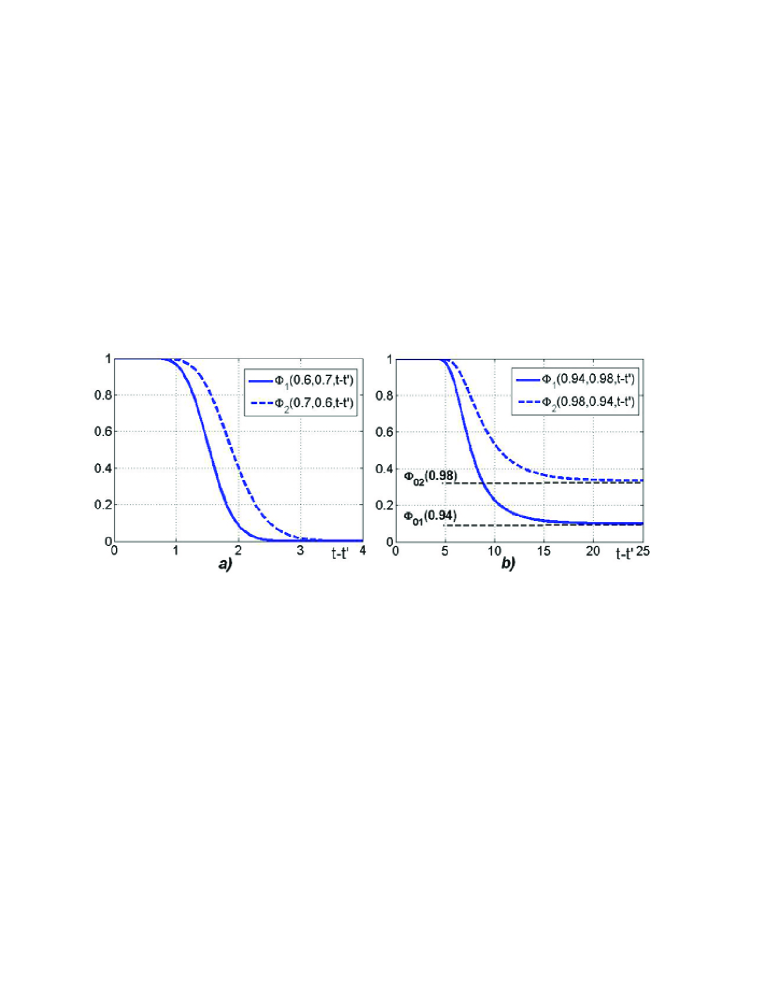
When the previous incoming spike and the current one are close in time to each other, the difference $(t-t^{\prime})$ is very small. It can be almost equal to zero (simultaneous spikes). In such a case we deal with the maximum of $Prob\left\{\zeta(t)\geq(v_{th}-k_{1}-k_{2}e^{-\mu(t-t^{\prime})})/\sqrt{D}\right\}$.

On the other hand, when $(t-t^{\prime})$ is large (long period between the previous and the current incoming spikes), we find, that:

$$\begin{array}[]{l}Prob\left\{\zeta(t)\geq(v_{th}-k_{1}-k_{2}e^{-\mu(t-t^{\prime})})/\sqrt{D}\right\}\to\\ \to Prob\left\{\zeta(t)\geq(v_{th}-k_{1})/\sqrt{D}\right\},\end{array}$$

and this is the minimum of considering probability as a function of difference $t-t^{\prime}$.

Denoting

$$\begin{array}[]{l}Prob\left\{\zeta(t)\geq(v_{th}-k_{i}-k_{j}e^{-\mu(t-t^{\prime})})/\sqrt{D}\right\}=\\ \qquad=\Phi_{i}(k_{i},k_{j},t-t^{\prime})\\ {\rm and}\\ Prob\left\{\zeta(t)\geq(v_{th}-k_{i})/\sqrt{D}\right\}=\Phi_{0i}(k_{i})\end{array}$$ (5)

we can rewrite Eq. (4) as:

$$\begin{array}[]{l}\rho_{3}(t)=\rho_{1}(t)\Phi_{01}(k_{1})+\rho_{2}(t)\Phi_{02}(k_{2})+\\ \\ \qquad+\rho_{1}(t)\left(1-\Phi_{02}(k_{2})\right)\int\limits_{t-T_{2}}^{t}\rho_{2}(t^{\prime})\Phi_{1}(k_{1},k_{2},t-t^{\prime})dt^{\prime}+\\ \\ \qquad+\rho_{2}(t)\left(1-\Phi_{01}(k_{1})\right)\int\limits_{t-T_{1}}^{t}\rho_{1}(t^{\prime})\Phi_{2}(k_{2},k_{1},t-t^{\prime})dt^{\prime},\end{array}$$ (6)

where

$$T_{1,2}=\frac{1}{\mu}\ln\left(\frac{k_{1,2}}{\sqrt{D}}\right).$$

The $\Phi_{1,2}(k_{1,2},k_{2,1},t-t^{\prime})$ factors are depicted at the Fig. 2 as functions of the time difference $t-t^{\prime}$.

Figure 2: Interaction functions introduced in Eq. (5) for weak and strong connections: a) – weak connections: $k_{1}=0.6$, $k_{2}=0.7$. There is a rather sharp boundary of a time period, when the second incoming spike is able to finish the ”work” of the previous one. The separate sensor’s spike is not practically able to fire the output neuron; b) – strong connections: $k_{1}=0.94$, $k_{2}=0.98$. It is easy to see that any separate spike is able to make fire the output neuron.

III.4 One more important multiplier

Regardless of shapes of $\rho_{1,2}(t)$ the FPTPD $\rho_{3}(t)$ must have one important characteristics: if the output neuron spike appears at some earlier time, then this circumstance decreases the probability of the spike in all later moments. We can reflect such a property by multiplying $\rho_{3}(t)$ by

$$\left(1-\int\limits_{0}^{t}\rho_{3}(t^{\prime})dt^{\prime}\right).$$

The problem is that our $\rho_{3}(t)$ may occur to be not normalized after the previous calculations (we explain it below, in the section IV.2). But it is possible (without losing of generality and facing with any contradictions) first to obtain $\rho_{3}(t)$ as described above, then normalize it, and then multiply the result by the mentioned multiplier:

$${\hat{\rho}}_{3}(t)={\tilde{\rho}}_{3}(t)\left(1-\int\limits_{0}^{t}{\tilde{\rho}}_{3}(t^{\prime})dt^{\prime}\right),$$ (7)

where ${\tilde{\rho}}_{3}(t)$ – is the normalized probability distribution.

III.5 A set of the interneuron states

Now we should recall that all previous calculations are valid until the first spike is generated by the $3^{rd}$ neuron. The question is: what happens after?

At the moment of the $3^{rd}$ neuron’s spike generation its membrane potential $v(t)$ is reset to initial value $v^{0}$, and the interneuron ”forgets” all previous history. We suppose that the $3^{rd}$ neuron spike is evoked by a spike of the $1^{st}$ or the $2^{nd}$ sensor exactly at the same moment. Let it be the $1^{st}$ sensor, which makes fire the output neuron. It is also reset to its initial membrane potential value $v_{1}^{0}$. Consequently, after reset FPTPD $\rho_{1}(t)$ has the same shape as it was previously. The other sensor is not reset simultaneously with $v_{1}(t)$ and $v(t)$. Therefore, its FPTPD $\rho_{2}(t)$ is shifted now in comparison with the initial situation. The Eq. (6) is valid, but now it provides us with new FPTPD $\rho_{3}^{(1)}(t)$, where the index $(.)^{(0)}$ is used for the initial situation. The time is measured now since the moment of last spike generation by the interneuron. The same is correct after each reset of the interneuron: one of $\rho_{1,2}(t)$ is similar to its initial form, while another one is shifted to the left or right. Hereafter we say that the output neuron gets into some state after each reset. These states are defined by corresponding shifts of FPTPDs $\rho_{1,2}(t)$ from the ”viewpoint” of the Eq. (6). For detailed description see the section IV.2. In the case of sinusoidal inputs and a finite number of sensors we have a finite number of these states. Hence, the resulting FPTPD of the output neuron should be written as

$$\begin{array}[]{l}\rho_{out}(t)=a_{0}{\hat{\rho}}_{3}^{(0)}(t)+a_{1}{\hat{\rho}}_{3}^{(1)}(t)+\\ \qquad+a_{2}{\hat{\rho}}_{3}^{(2)}(t)+\dots+a_{M-1}{\hat{\rho}}_{3}^{(M-1)}(t),\end{array}$$

where $M$ is a whole number of the interneuron’s states. The coefficients $a_{k}$ denote relative frequencies of switching into according states. We talk about values of these coefficients below in the section IV.2. Since the distribution ${\hat{\rho}}_{3}^{(k)}(t)$ is particular for the $k^{th}$ state, it would be incorrect to use here $\rho_{3}^{(k)}(t)$ (without a hat) and then to perform the same operation as in Eq. (7).

III.6 Example for different frequencies of sinusoidal inputs

Let’s take two sensors with input sinusoidal signals of different frequencies $\Omega_{1}\neq\Omega_{2}$. We only suppose, that these frequencies are in a ratio of some integers $m$ and $n$, i.e. $\Omega_{1}/\Omega_{2}=m/n$. This means that the first $(m-1)$ peaks of $\rho_{1}(t)$ don’t coincide with the first $(n-1)$ peaks of $\rho_{2}(t)$. And the $m^{th}$ peak of $\rho_{1}(t)$ coincides with the $n^{th}$ peak of $\rho_{2}(t)$.

Consequently, the output neuron has $M=(m-1)+(n-1)+1=m+n-1$ different possible states against peaks of $\rho_{1,2}(t)$, i.e. if it is reset together with any spike of the first or the second sensor, then since the reset time there is always only one of $M$ different variants of an incoming spike train (the superposition of spike sequences from both sensors) with a definite probability density in time for each incoming spike.

IV Numerical experiments

IV.1 Consonance and Dissonance in music

The sinusoidal signal is considered to be the simplest one in an investigation of different systems. May be the first level of complication is the linear combination of two sinusoidal signals of different frequencies. And here we face with the set of very old questions related with musical accords.

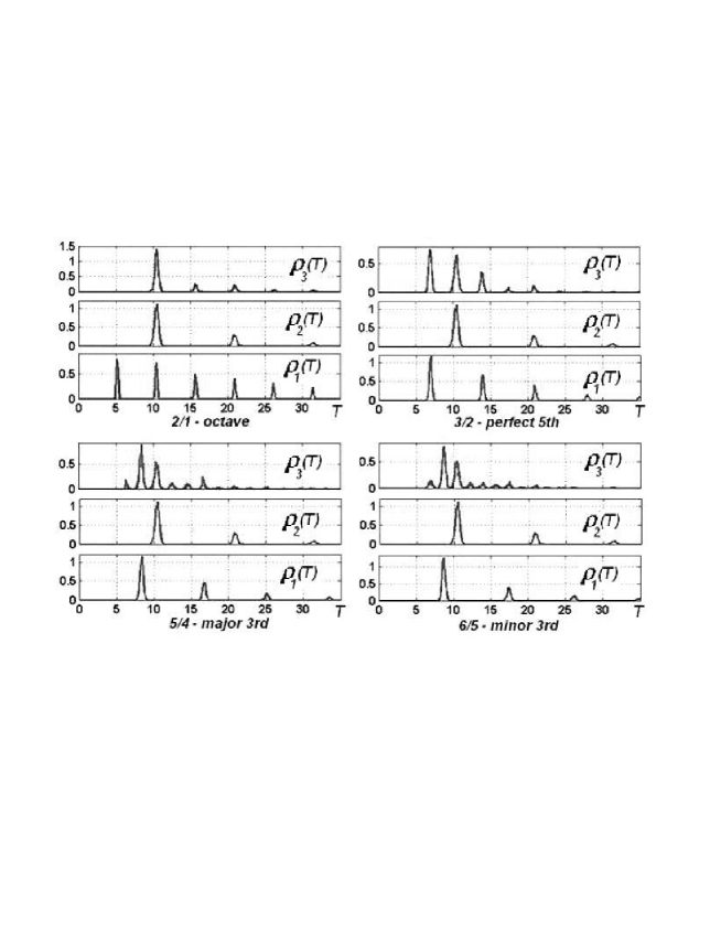
The Pythagoreans discovered that the accord of two sinusoidal signals sounds pleasant (consonant) if their frequencies ratio is $m/n$, where $m$ and $n$ are the small integers (e.g. $2/1$, $3/2$, $4/3$) Plomp and Levelt (1965). Conversely, if $m$ and $n$ are the large numbers (e.g. $45/32$), then the accord sounds dissonant, i.e. unpleasant.

In the context of our investigation it is really interesting, how the dissonance and the consonance are mapped to ISI distributions.

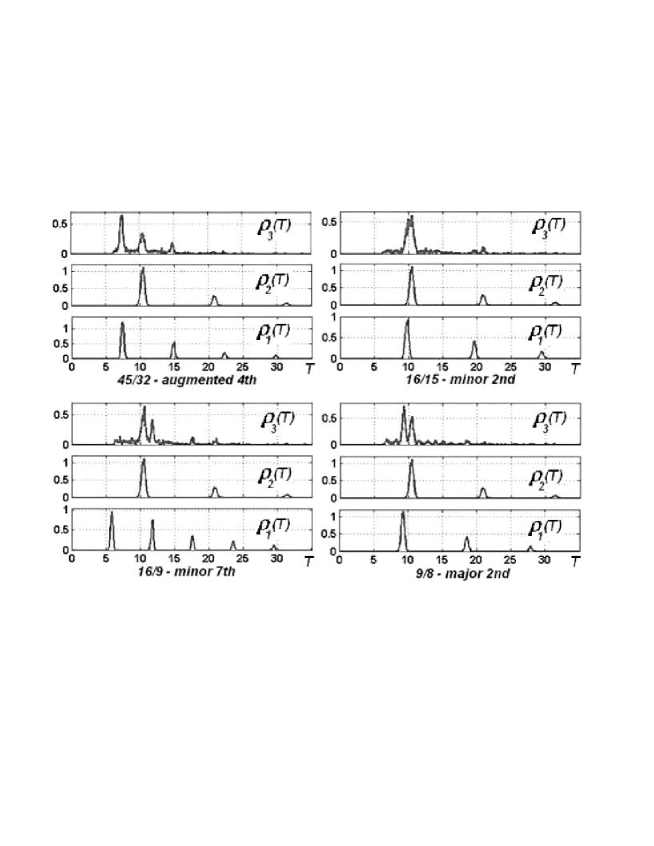
In the Figs. 3 and 4 there are the distributions for consonant and dissonant accords, respectively. It is easy to see the higher integers $m,n$ the regularity less in an appropriate distribution of ISI, although the structure of the input signal is in principal the same: two sinusoids. These curves are obtained through the direct numerical simulations of the system Eq. (1). The theoretical part of our work is focused on building a basis for the simulations results.

Figure 3: The consonant accords: under each picture there is the ratio of frequencies ($m/n$) and the name of the accord used in the common musical terminology. All curves are obtained through the direct numerical simulation of the system Eq. (1) with $\Omega_{2}=0.6$, $A_{2}=1.165$, $\Omega_{1}=(m/n)\Omega_{2}$, and $A_{1}$ according the subthreshold input sinusoidal signal condition Eq. (3).

Figure 4: The dissonant accords: under each picture there is the ratio of frequencies ($m/n$) and the name of the accord used in the common musical terminology. All curves are obtained through the direct numerical simulation of the system Eq. (1) with $\Omega_{2}=0.6$, $A_{2}=1.165$, $\Omega_{1}=(m/n)\Omega_{2}$, and $A_{1}$ specified by the subthreshold input sinusoidal signal condition Eq. (3).

IV.2 Verification of theoretical conclusions

The formula (6) is obtained under a set of assumptions. So, this theoretical result should be compared with the results of numerical experiments. Here we present the idea of usage of the expression and check its validity.

Let’s take, for instance, the ”Perfect $4^{th}$” accord, which consists of 2 sinusoids of frequencies related by the ratio $\Omega_{1}/\Omega_{2}=4/3$.

The FPTPDs $\rho_{1}(t)$ and $\rho_{2}(t)$ are known to us from the numerical simulations of sensors, for example. If the figures of these distributions are placed in a column (Fig. 5, State 0), then it is easy to see, that the $3^{rd}$ peak of $\rho_{2}(t)$ coincides with the $4^{th}$ peak of $\rho_{1}(t)$. All other peaks don’t coincide, and (as it is explained in the section III.6) here we have $4+3-1=6$ different possible states of the $3^{rd}$ neuron: State 0, State 1, …, and State 5. Let’s establish the correspondence between these states and the peaks of $\rho_{1,2}(t)$ as it is shown on the Fig. 5: numbers of the states are placed into circles. Area under each peak means the probability to find an incoming spike at the defined short period of time. If this spike evokes the spike of the $3^{rd}$ neuron, it is switched into the appropriate state.

Figure 5: FPTPDs of three neurons in the states 0 and 1. This is the example of the probable transition between two states for the case of input sinusoids with frequencies related by ratio $4/3$ (the Perfect $4^{th}$ accord). $\rho_{2}(t)$ is shifted in the State 1 in comparison with $\rho_{2}(t)$ in the State 0. As a result, $\rho_{3}^{(0)}(t)$ and $\rho_{3}^{(1)}(t)$ are different. All possible states of the interneuron are: State 0, State 1, …, and State 5. The peaks of $\rho_{1,2}(t)$ are marked by numbers in circles in order to establish the correspondence between them and the interneuron states.

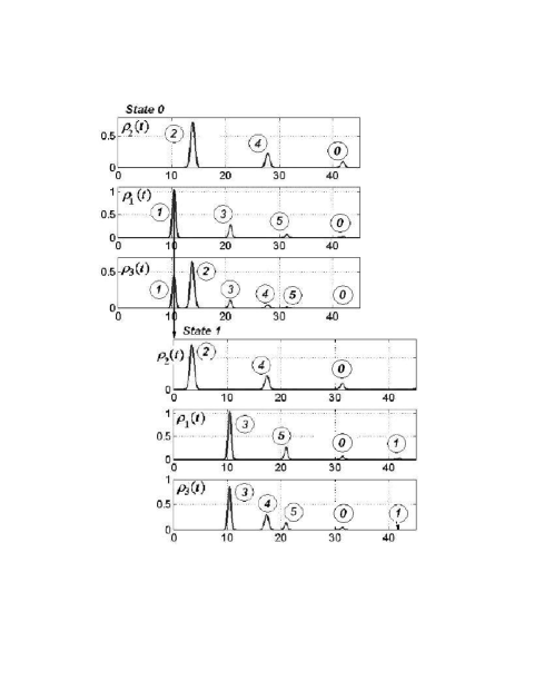
Initially all three neurons are reset. This is the $0^{th}$ state. The most probable and close in time spike comes from the $1^{st}$ sensor (Fig. 5). If this spike makes fire the interneuron, then it is switched into the $1^{st}$ state, where the most probable and close spike comes from the $2^{nd}$ sensor. Obviously, this spike (if it is generated) comes during the refractory period, so, the closest valuable spike in the $1^{st}$ state comes again from the $1^{st}$ sensor and has the possibility to switch the interneuron into the $3^{rd}$ state, and etc.

Here we recall the section III.4 and notice that the peak of $\rho_{1}(t)$ or $\rho_{2}(t)$, which appears during the refractory period, is the main reason why we may find $\rho_{3}(t)$ to be not normalized in Eq. (4). This ”invisible” to the output neuron peak does not contribute into the $\rho_{3}(t)$ peaks, but it is the big meaningful part of an appropriate normalized sensor’s FPTPD.

The analysis of $\rho_{3}(t)$ peaks in each state shows that in the case of musical accords and strong connections the interneuron gets into all possible $m+n-1$ states almost uniformly, i.e. all states make almost equal contributions into the common $\rho_{out}(t)$.

Therefore, the simplest way to obtain the final output distribution is to directly sum all ${\hat{\rho}}_{3}^{(k)}(t)$ and then to normalize this result. In other words, all coefficients $a_{k}$ (see the section III.5) can be set to unit:

$$\rho_{out}(t)=\frac{\sum\limits_{k=1}^{M}{\hat{\rho}}_{3}^{(k)}(t)}{\int\limits_{0}^{\infty}dt^{\prime}\sum\limits_{k=1}^{M}{\hat{\rho}}_{3}^{(k)}(t^{\prime})}.$$ (8)

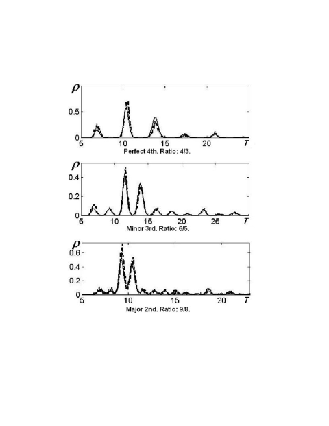
These approximate conclusions provide $\rho_{out}(t)$ curves very similar to ones obtained through direct numerical calculations of the system (1). The examples of compared results are shown in the Fig. 6.

Figure 6: ISI distributions of the output neuron for different accords. Solid line is the theoretical result. Dashed line is the distribution obtained throughout the direct numerical simulation of the system (1). The parameters are $\mu_{1}=\mu_{2}=1$, $\mu=0.3665$, $k_{1}=k_{2}=0.97$, $D_{1}=D_{2}=D=1.6\cdot 10^{-3}$. Perfect 4th: $A_{1}=1.165$, $\Omega_{1}=0.6$, $A_{2}=1.085$, $\Omega_{2}=0.45$. Minor 3rd: $A_{1}=1.125$, $\Omega_{1}=0.54$, $A_{2}=1.085$, $\Omega_{2}=0.45$. Major 2nd: $A_{1}=1.2$, $\Omega_{1}=0.675$, $A_{2}=1.165$, $\Omega_{2}=0.6$.

V The calculation algorithm

Summarizing the previous sections, let’s present the described theoretical approach in the form of the calculation algorithm. Thus, in order to obtain the interneuron’s ISID curve under chosen parameters of the system Eq. (1) we should perform the following steps.

1. To obtain the sensors’ FPTPDs $\rho_{1,2}(t)$ using the direct numerical simulation of the system Eq. (1) without the interneuron, or theoretical approaches described in Ref. Burkitt (2006).

2. To find all possible States of the interneuron against the peaks of $\rho_{1,2}(t)$ (see Fig. 5 for example).

3. To calculate $\hat{\rho}_{3}^{(i)}(t)$ in each State using Eqs. (6, 7).

4. And, finally, to sum and normalize the calculated $\hat{\rho}_{3}^{(i)}(t)$ in accordance with Eq. (8).

Despite of the relative complexity of the algorithm, its usage decreases consumption of resources necessary for smooth interneuron’s ISID obtaining. It allows also to perform fast estimations and provides anyhow the consistent theoretical description of the noisy nonlinear system Eq. (1).

VI Hypotheses of consonance and dissonance

There is a few of main hypotheses explaining why animals, including humans, feel harmony or disharmony listening to different tones combinations. We suppose that the input signals, which are transformed into spike trains with blurred, i.e. noise-like Interspike Intervals Distributions, are felt unpleasant (dissonant, inharmonious) due to the analysis, recognition and survival in noisy environment of the brain problems.

Let’s try to understand the correlation between that viewpoint and some other hypotheses of the dissonance.

Helmholtz (1877) Helmholtz (1954) proposed the notion that dissonance arises due to beating between adjacent harmonics of complex tones. In effect, dissonance arises due to rapid amplitude fluctuations.

It is possible to prove mathematically that, if the input frequencies into our system are in ratio $\Omega_{1}/\Omega_{2}=m/n$ (where $m>n$), then the minimal distance between peaks of $\rho_{3}^{(i)}(t)$ is $T_{min}=(2\pi/\Omega_{2})/m=T_{2}/m$ (see the Fig. 5: the peaks 1, 2 of the $\rho_{3}^{(0)}(t)$, and the peaks 4, 5 of the $\rho_{3}^{(1)}(t)$) that defines the distance between peaks of the final ISID $\rho_{out}(t)$. That’s why the sufficiently high value of $m$ means the blurred ISID, typical for dissonant accords. In such a way, we show that even for pure input tones, and even if they are not close in frequency in order to produce beats, we may feel the dissonance. Hence, the hypothesis by Helmholtz continues to be correct, if we look at the minimal distance among all peaks of $\rho_{1}(t)$ and $\rho_{2}(t)$, and not only the firsts ones, which show the difference between the input tones’ frequencies.

Another theory is the Long Pattern Hypothesis from Boomsliter and Creel (1961) Boomsliter and Creel (1961) which states that a consonance is based on the length of the overall period of a stimulus. They show that consonant intervals, based on simple integer ratios of fundamental frequencies, have shorter overall periods than do dissonant intervals.

Indeed, as we obtain for our model, the higher integers are $m$ and $n$, the higher number of states ($m+n-1$) the interneuron has against the pattern of $\rho_{1,2}(t)$ peaks. In fact, the sequence of the states repeats periodically in time with the period $T_{state}=(2\pi/\Omega_{1})m=(2\pi/\Omega_{2})n$, which is the period of phases coincidences of $\cos\Omega_{1}t$ and $\cos\Omega_{2}t$, i.e. the overall period. But the interneuron gets into each state randomly. So, for the high number of states (dissonance) it is necessary much time in order to recognize some regularity inherent to the output spike train. Conversely, in the case of consonant input, the same amount of the spike train statistics details can be acquired in shorter periods of observation. Thus, the consonant inputs are in the priority against the dissonant ones, from the analysis viewpoint.

VII Discussion and conclusions

In the work we try to follow a signal propagating throughout the neural-like system. The second layer of the system doesn’t allow applying the framework of Markovian processes. Nevertheless, we propose the qualitative analysis yielding the main result of the work: the analytical expressions and the consistent algorithm applicable for an investigation of the ISI statistics and its transformations.

The proposed algorithm is ready to be used for quick estimations of output distributions because of step-like shapes of the functions called ”$\Phi(\dots)$” and narrow peaks of FPTPDs $\rho_{1}(t)$ and $\rho_{2}(t)$.

On the other hand, the found procedure is clear enough to be implemented in the widely used programming environments. In such an implementation it provides a rather precise approximation (see the Fig. 6) of the output ISI distribution (ISID) given by the direct computer simulation of Eq. (1). We should also emphasize that in order to obtain a smooth curve of the ISID, using the direct numerical simulation of the system (1), it is necessary to consume much more temporal, soft- and hard-ware resources than in the case of a program implementation of the proposed algorithm usage.

In the simple case of the auditory system model we are able to discover existence of some accords (a combination of two sinusoidal signals), which evoke ISIDs blurring very fast with propagation from one neural layer to another (Fig. 4). And in our study these accords are the same as the dissonant ones in music, i.e. the dissonant accords are the ones, which are not able to ”survive” in the noisy neural environment after a number of interneurons layers.

We also show that from the perceptional point of view the dissonant accord’s ISI statistics needs more time to be collected in comparison with the consonant accord’s one. The latter one evokes a sharp ISID’s shape, which is able to ”survive” a number of proposed transformations, i.e. the same algorithm is applicable in order to understand what happens to the consonant accords on deeper layers of the neural system.

As it is easy to see the output ISID contains peaks corresponding to quasi-periodical spike generation at frequencies, which are absent in the input signal. So, it is possible and intersting to investigate the Ghost Stochastic Resonance phenomenon Balenzuela (2005); Chialvo et al. (2002) in details for this model. However, the current paper is focused on the theoretical approach to the whole ISID picture shaping. All sophisticated tuning of coupling coefficients, input frequencies, and noise intensities can be performed separately in a sake of resonances investigation, and this analysis can be also augmented by results revealed from the proposed analytical approach.

The obtained results may be applied also in the context of such recent studies as, for example, the stimulus reconstruction from neural spike trains, where the information transmission under the noise influence is investigated Nikitin et al. (2007). The other suitable context of these results application is the continuous investigation of the neuron’s behavior under the influence of a constant bombardment of inhibitory and excitatory postsynaptic potentials somehow resembling a background noise that is typical for functioning conditions of, for example, the neocortical neurons Luccioli et al. (2006).

References

- Gammaitoni et al. (1998) L. Gammaitoni, P. Hanggi, P. Jung, and F. Marchesoni, Rev. Mod. Phys. 70, 228 (1998).
- Gerstner and Kistler (2002) W. Gerstner and W. Kistler, Spiking Neuron Models. Single Neurons, Populations, Plasticity (Cambridge University Press, 2002).
- Longtin et al. (2008) A. Longtin, J. W. Middleton, J. Cieniak, and L. Maler, Mathematical Biosciences 214, 87 (2008).
- Fishman et al. (2001) Y. I. Fishman, I. O. Volkov, M. D. Noh, P. C. Garell, H. Bakken, J. C. Arezzo, M. A. Howard, and M. Steinschneider, J Neurophysiol 86, 2761 (2001).
- Helmholtz (1954) H. L. F. Helmholtz, On the sensations of tone (Dover, New York, 1954).
- Burkitt (2006) A. N. Burkitt, Biol. Cybern. 95, 97 (2006).
- Balenzuela (2005) P. Balenzuela, Chaos 15, 023903 (2005).
- Lopera et al. (2006) A. Lopera, J. Buldu, M. Torrent, D. Chialvo, and J. Garcia-Ojalvo, Phys. Rev. E 73, 021101 (2006).
- Chialvo et al. (2002) D. Chialvo, O. Calvo, D. Gonzalez, O. Piro, and G. Savino, Phys. Rev. E 65, 050902 (2002).
- Plomp and Levelt (1965) R. Plomp and W. J. M. Levelt, Journal of the Acoustical Society of America 38, 548 (1965).
- Cox (1967) D. Cox, Renewal theory (Chapman and Hall, 1967).
- Gardiner (1985) C. W. Gardiner, Handbook of stochastic methods (Springer, 1985), 2nd ed.
- Boomsliter and Creel (1961) P. Boomsliter and W. Creel, J. Music Theory 5, 2 (1961).
- Nikitin et al. (2007) A. Nikitin, N. G. Stocks, and R. P. Morse, Phys. Rev. E 75, 021121 (2007).
- Luccioli et al. (2006) S. Luccioli, T. Kreuz, and A. Torcini, Phys. Rev. E 73, 041902 (2006).