SINGLE MESON PRODUCTION IN PHOTON-PHOTON COLLISIONS AND INFRARED RENORMALONS

Abstract

In this article, we investigate the contribution of the higher-twist Feynman diagrams to the large-$p_{T}$ inclusive single meson production cross section in photon-photon collisions and present the general formulas for the higher-twist differential cross sections in case of the running coupling and frozen coupling approaches. The structure of infrared renormalon singularities of the higher-twist subprocess cross section and the resummed expression (the Borel sum) for it are found. We compared the resummed higher-twist cross sections with the ones obtained in the framework of the frozen coupling approach and leading-twist cross section. We obtain, that ratio $R=(\Sigma_{M^{+}}^{HT})^{res}$/$(\Sigma_{M^{+}}^{HT})^{0}$, for all values of the transverse momentum $p_{T}$ of the meson identically equivalent to ratio $r$=($\Delta_{M}^{HT})^{res}$/$(\Delta_{M}^{HT})^{0}$. It is shown that the resummed result depends on the choice of the meson wave functions used in calculation. Phenomenological effects of the obtained results are discussed.

I Introduction

Exclusive processes involving large momentum transfer are among the most interesting and challenging test of quantum chromodynamics (QCD). The framework for analyzing such processes within the context of perturbative QCD (pQCD) has been developed by Brodsky and Lepage [1,2], Efremov and Radyshkin [3], and Duncan and Mueller [4]. They have demonstrated, to all orders in perturbation theory, that exclusive amplitudes involving large momentum transfer factorize into a convolution of a process-independent and perturbatively incalculable distribution amplitude, one for each hadron involved in the amplitude, with a process-dependent and perturbatively calculable hard-scattering amplitude.

The hadronic wave function in terms of quark and gluon degrees of freedoms plays an important role in QCD process predictions. For example, knowledge of the wave function allows to calculate distribution amplitudes and structure functions or conversely these processes can give phenomenological restrictions on the wave functions.

During the last few years, a great deal of progress has been made in the investigation of the properties of hadronic wave functions[5-17].

The standard approach to distribution amplitudes, which is due to Brodsky and Lepage[14], considers the hadron’s parton decomposition in the infinite momentum frame. A conceptually different, but mathematically equivalent formalism is the light-cone quantization[15]. Either way, power-suppressed contributions to exclusive processes in QCD, which are commonly referred to as higher-twist corrections. The higher-twist approximation describes the multiple scattering of a parton as power corrections to the leading-twist cross section.

Among the fundamental predictions of QCD are asymptotic scaling laws for large-angle exclusive processes [18-22]. QCD counting rules were formalized in Refs.[19,20].

The frozen coupling constant approach can be applied for investigation, not only exclusive processes, but also for the calculation of higher-twist contributions to some inclusive processes, for example as large -$p_{T}$ meson photoproduction [23], two-jet+meson production in the electron-positron annihilation [24]. In the works [24,25] for calculation of integrals, such as

$$I\sim\int\frac{\alpha_{s}(\hat{Q}^{2})\Phi(x,\hat{Q}^{2})}{1-x}dx$$ (1)

the frozen coupling constant approach was used. According to Ref.[25] should be noted that in pQCD calculations the argument of the running coupling constant in both, the renormalization and factorization scale $\hat{Q}^{2}$ should be taken equal to the square of the momentum transfer of a hard gluon in a corresponding Feynman diagram. But defined in this way, $\alpha_{s}(\hat{Q}^{2})$ suffers from infrared singularities. For example in our work [26], $\hat{Q}^{2}$ equals to $x_{2}\hat{s}$ and $-x_{1}\hat{u}$, where $\hat{s}$, $\hat{u}$ are the subprocess’s Mandelstam invariants. Therefore, in the soft regions $x\rightarrow 0$, integrals (1.1) diverge and for their calculation some regularization methods of $\alpha_{s}(Q^{2})$ in these regions are needed. In Ref.[27], the authors investigated the phenomenology of infrared renormalons in inclusive processes. The dispersive approach has been devised to extend properly modified perturbation theory calculations towards the low-energy region [28]. Connections between power corrections for the three Deep Inelastic Scattering sum rules have also been explored in [29].

Investigation of the infrared renormalon effects in various inclusive and exclusive processes is one of the most important and interesting problems in the perturbative QCD. As we know the word ”renormalon” first appeared in Ref.[30]. A singularity in the Borel parameter- is called a renormalon. It is known that infrared renormalons are responsible for factorial growth of coefficients in perturbative series for the physical quantities. But, these divergent series can be resummed by means of the Borel transformation [30] and the principal value prescription [31], and effects of infrared renormalons can be taken into account by a scale-setting procedure $\alpha_{s}(Q^{2})\rightarrow\alpha_{s}(exp(f(Q^{2}))Q^{2})$ at the one-loop order results. Technically, all-order resummation of infrared renormalons corresponds to the calculation of the one-loop Feynman diagrams with the running coupling constant $\alpha_{s}(-k^{2})$ at the vertices or, alternatively, to calculation of the same diagrams with nonzero gluon mass. Studies of infrared renormalon problems have also opened new prospects for evaluation of power-suppressed corrections to processes characteristics [32]. Power corrections can also be obtained by means of the Landau-pole free expression for the QCD coupling constant. The most simple and elaborated variant of the dispersive approach, the Shirkov and Solovtsov analytic perturbation theory, was formulated in Ref.[33]. The $k_{T}$ factorization theorem has been widely applied to inclusive and exclusive processes in perturbative QCD. This theorem holds for simple processes, such as deeply inelastic scattering (DIS) and Drell-Yan production[34].

A full twist 3 treatment of $\rho$-electroproduction in $k_{T}$ -factorisation is possible[35]. It relies on the computation of the $\gamma_{T}^{\ast}-\rho_{T}$ impact factor at twist 3 including consistently all twist 3 contributions, i.e. 2-parton and 3-parton correlators. This gives a gauge invariant impact factor, and an amplitude which is free of end-point singularities due to the presence of $k_{T}$ .

An additional, general property is that the singularities in $B[u]$ occur at integer-and sometimes half integer-values of $u$. This corresponds to the fact that alternative definitions of the sum of the series differ by integer-or half integer-power of $\Lambda^{2}/Q^{2}$. These ambiguities must be cancelled by nonperturbative power corrections, and they can therefore serve as a perturbative probe of such effects. In the absence of an operator product expansion, the renormalon technique often provides a unique window into the nonperturbative regime: by identifying the ambiguities in summing the perturbative series one learns about the parametric dependence of power corrections on the hard scales and about their potential size[36].

By taking these points into account, it may be argued that the analysis of the higher-twist effects on the dependence of the meson wave function in single pseudoscalar and vector meson production at photon-photon collisions by the running coupling (RC) approach are significant from both theoretical and experimental points of view.

In this work we will apply the running coupling approach[37] in order to compute effects of the infrared renormalons on the meson production in photon-photon collisions. This approach was employed also in our work[38] for calculation of the single meson production in proton-proton collisions.

Photon-photon collisions represent a very useful tool for the study of hadron production. Basically, the more attractive feature is the simple, clean initial state, involving only QED interactions, which allows one to concentrates on the final hadronic state. This way, in fact, some of the more clean tests for pQCD models were proposed [14]. It is well known that exclusive $\gamma\gamma\to hadron$ processes can be studied in the $e^{+}e^{-}$ colliders, particularly $\gamma^{*}\gamma^{*}$ processes, play a spesial role in QCD [39], since their analysis is under much better control than the calculation of hadronic processes, which requre the input of non-perturbative hadronic structure functions or wave functions.

A precise measurement of the inclusive charged meson production cross section at $\sqrt{s}=183GeV$ and $\sqrt{s}=209GeV$ is important for the photon-photon collisions program at the International Linear Collider (ILC). The results of our calculations are based on the photon-photon collisions at $\sqrt{s}=183GeV$ and $\sqrt{s}=209GeV$.

The higher-twist contributions to high-$p_{T}$ inclusive meson production in two-photon collisions, a single meson inclusive photoproduction and jet photoproduction cross sections were studied by various authors [40-42]. As experiments examining high-$p_{T}$ particle production in two-photon collisions are improved, it becomes important to reassess the various contributions which arise in quantum chromodynamics. Predicting for the higher-twist contributions, originally obtained in Ref.43, may now be refined using the exclusive-process QCD formalism devoloped in [44]. Another important aspect of this study is the choice of the meson model wave functions. In this respect, the contribution of the higher-twist Feynman diagrams to a single meson production cross section in photon-photon collisions has been computed by using various meson wave functions. Also, the leading and higher-twist contributions have been estimated and compared to each other. Within this context, this paper is organized as follows: in Sec. II, we provide some formulas for the calculation of the contribution of the high twist diagrams. In Sec. III we present formulas and an analysis of the higher-twist effects on the dependence of the meson wave function by the running coupling constant approach. In Sec. IV, we provide the formulas for the calculation of the contribution of the leading-twist diagrams and in Sec. V, we present the numerical results for the cross section and discuss the dependence of the cross section on the meson wave functions. We state our conclusions in section VI.

II CONTRIBUTION OF THE HIGH TWIST DIAGRAMS

The higher-twist Feynman diagrams, which describe the subprocess $\gamma q\to Mq$ contributes to $\gamma\gamma\to MX$ for the meson production in the photon-photon collision are shown in Fig.1(a). The amplitude for this subprocess can be found by means of the Brodsky-Lepage formula [45]

$$M(\hat{s},\hat{t})=\int_{0}^{1}{dx_{1}}\int_{0}^{1}dx_{2}\delta(1-x_{1}-x_{2})\Phi_{M}(x_{1},x_{2},Q^{2})T_{H}(\hat{s},\hat{t};x_{1},x_{2}).$$ (2)

In Eq.(2.1), $T_{H}$ is the sum of the graphs contributing to the hard-scattering part of the subprocess. The hard-scattering part for the subprocess under consideration is $\gamma q_{1}\to(q_{1}\overline{q}_{2})q_{2}$, where a quark and antiquark form a pseudoscalar, color-singlet state $(q_{1}\bar{q}_{2})$. Here $\Phi(x_{1},x_{2},Q^{2})$ is the meson wave function, i.e., the probability amplitude for finding the valence $q_{1}\bar{q}_{2}$ Fock state in the meson carry fractions $x_{1}$ and $x_{2}$, $x_{1}+x_{2}=1$. Remarkably, this factorization is gauge invariant and only requires that the momentum transfers in $T_{H}$ be large compared to the intrinsic mass scales of QCD. Since the distribution amplitude and the hard scattering amplitude are defined without reference to the perturbation theory, the factorization is valid to leading order in $1/Q$, independent of the convergence of perturbative expansions. The Hard-scattering amplitude $T_{H}$ can be calculated in perturbation theory and represented as a series in the QCD running coupling constant $\alpha_{s}(Q^{2})$.

The $q_{1}\overline{q}_{2}$ spin state used in computing $T_{H}$ may be written in the form

$$\sum_{s_{1},s_{2}}\frac{u_{s_{1}}({x}_{1}p_{M})\overline{v}_{s_{2}}({x}_{2}p_{M})}{\sqrt{x_{1}}\sqrt{x_{2}}}\cdot N_{s_{1}s_{2}}^{s}=\left\{\begin{array}[]{ccc}\frac{{\gamma}_{5}\hat{p}_{\pi}}{\sqrt{2}},\,\,\pi,\\ \frac{\hat{p}_{M}}{\sqrt{2}},\,\,\rho_{L}\,\,helicity\,0,\\ \mp\frac{{\varepsilon}_{\mp}\hat{p}_{M}}{\sqrt{2}},\,\,\rho{{}_{T}}\,\,helicity\pm 1,\end{array}\right.$$ (3)

where $\varepsilon_{\pm}=\mp(1/\sqrt{2})(0,1,\pm i,0)$ in a frame with $(p_{M})_{1,2}=0$ and the $N_{s_{1}s_{2}}^{s}$ project out a state of spins $s$, and $p_{M}$ is the four-momentum of the final meson. In our calculation, we have neglected the meson mass. Turning to extracting the contributions of the higher-twist subprocesses, there are many kinds of leading-twist subprocesses in $\gamma\gamma$ collisions as the background of the higher-twist subprocess $\gamma q\to Mq$, such as $\gamma+\gamma\to q+\overline{q}$. The contributions from these leading-twist subprocesses strongly depend on some phenomenological factors, for example, quark and gluon distribution functions in meson and fragmentation functions of various constituents etc. Most of these factors have not been well determined, neither theoretically nor experimentally. Thus they cause very large uncertainty in the computation of the cross section of process $\gamma\gamma\to MX$. In general, the magnitude of this uncertainty is much larger than the sum of all the higher-twist contributions, so it is very difficult to extract the higher-twist contributions.

The Mandelstam invariant variables for subprocesses $\gamma q\to Mq$ are defined as

$$\hat{s}=(p_{1}+p_{\gamma})^{2},\quad\hat{t}=(p_{\gamma}-p_{M})^{2},\quad\hat{u}=(p_{1}-p_{M})^{2}.$$ (4)

We have aimed to calculate the meson production cross section and to fix the differences due to the use of various meson model functions. We have used seven different wave functions: the asymptotic wave function (ASY), the Chernyak-Zhitnitsky wave function [6,9], the wave function in which two nontrivial Gegenbauer coefficients $a_{2}$ and $a_{4}$ have been extracted from the CLEO data on the $\gamma\gamma^{\star}\to\pi^{0}$ transition form factor [46], the Braun-Filyanov pion wave functions [11] and the Bakulev-Mikhailov-Stefanis pion wave function[47]. It should be noted that the wave functions of pions also are developed in Refs.[48-50] by the Dubna group. For $\rho$- meson wave function we used the Ball-Braun wave function[51].

$$\Phi_{asy}(x)=\sqrt{3}f_{\pi}x(1-x),\quad\Phi_{L(T)}^{asy}(x)=\sqrt{6}f_{\rho}^{L(T)}x(1-x),\\$$

$$\Phi_{CZ}(x,\mu_{0}^{2})=\Phi_{asy}(x)\left[C_{0}^{3/2}(2x-1)+\frac{2}{3}C_{2}^{3/2}(2x-1)\right],$$

$$\Phi_{L(T)}^{\rho}(x,\mu_{0}^{2})=\Phi_{L(T)}^{asy}(x)\left[C_{0}^{3/2}(2x-1)+0.18(0.2)\frac{2}{3}C_{2}^{3/2}(2x-1)\right],$$

$$\Phi_{BMS}(x,\mu_{0}^{2})=\Phi_{asy}(x)\left[C_{0}^{3/2}(2x-1)+0.188C_{2}^{3/2}(2x-1)-0.13C_{4}^{3/2}(2x-1)\right],$$

$$\Phi_{CLEO}(x,\mu_{0}^{2})=\Phi_{asy}(x)\left[C_{0}^{3/2}(2x-1)+0.27C_{2}^{3/2}(2x-1)-0.22C_{4}^{3/2}(2x-1)\right],$$

$$\Phi_{BF}(x,\mu_{0}^{2})=\Phi_{asy}(x)\left[C_{0}^{3/2}(2x-1)+0.44C_{2}^{3/2}(2x-1)+0.25C_{4}^{3/2}(2x-1)\right],$$ (5)

$$C_{0}^{3/2}(2x-1)=1,\,\,C_{2}^{3/2}(2x-1)=\frac{3}{2}(5(2x-1)^{2}-1),$$

$$C_{4}^{3/2}(2x-1)=\frac{15}{8}(21(2x-1)^{4}-14(2x-1)^{2}+1).$$

where $f_{\pi}=0.923GeV$, $f_{\rho}^{L}$=0.141 GeV$,f_{\rho}^{T}$=0.16 GeV are the pion and $\rho$ mesons decay constants. Here, we have denoted by $x\equiv x_{1}$, the longitudinal fractional momentum carried by the quark within the meson. Then, $x_{2}=1-x$ and $x_{1}-x_{2}=2x-1$. The pion and $\rho$ meson wave functions is symmetric under the replacement $x_{1}-x_{2}\leftrightarrow x_{2}-x_{1}$.

Several important nonperturbative tools have been developed which allow specific predictions for the hadronic wave functions directly from theory and experiments. The QCD sum-rule technique and lattice gauge theory provide constraints on the moments of the hadronic distribution amplitude. However, the correct meson wave function is still an open problem in QCD. It is known that the meson wave function can be expanded over the eigenfunctions of the one-loop Brodsky-Lepage equation, i.e., in terms of the Gegenbauer polynomials $\{C_{n}^{3/2}(2x-1)\},$

$$\Phi_{M}(x,Q^{2})=\Phi_{asy}(x)\left[1+\sum_{n=2..}^{\infty}a_{n}(Q^{2})C_{n}^{3/2}(2x-1)\right],$$ (6)

In the present work, we take into account the evolution of the meson wave function on the factorization scale. The evolution of the wave function on the factorization scale $Q^{2}$ is governed by the functions $a_{n}(Q^{2})$,

In the case $\pi$ meson,

$$a_{n}(Q^{2})=a_{n}(\mu_{0}^{2})\left[\frac{\alpha_{s}(Q^{2})}{\alpha_{s}(\mu_{0}^{2})}\right]^{\gamma_{n}/\beta_{0}},$$ (7)

$$\frac{\gamma_{2}}{\beta_{0}}=\frac{50}{81},\,\,\,\frac{\gamma_{4}}{\beta_{0}}=\frac{364}{405},\,\,n_{f}=3.$$

In Eq.(2.6), $\{\gamma_{n}\}$ are anomalous dimensions defined by the expression,

$$\gamma_{n}=C_{F}\left[1-\frac{2}{(n+1)(n+2)}+4\sum_{j=2}^{n+1}\frac{1}{j}\right].$$ (8)

In the case $\rho$ meson,

$$a_{n}(Q^{2})^{\|(\bot)}=a_{n}(\mu_{0}^{2})^{\|(\bot)}\left[\frac{\alpha_{s}(Q^{2})}{\alpha_{s}(\mu_{0}^{2})}\right]^{(\gamma_{n}^{\|(\bot)}-\gamma_{0})/(2\beta_{0})},$$ (9)

Here,

$$\gamma_{n}^{\|}=\frac{8}{3}\left[1-\frac{2}{(n+1)(n+2)}+4\sum_{j=2}^{n+1}\frac{1}{j}\right].$$

$$\gamma_{n}^{\bot}=\frac{8}{3}\left[1+4\sum_{j=2}^{n+1}\frac{1}{j}\right].$$

The constants $a_{n}(\mu_{0}^{2})=a_{n}^{0}$ are input parameters that form the shape of the wave functions and which can be extracted from experimental data or obtained from the nonperturbative QCD computations at the normalization point $\mu_{0}^{2}$. The QCD coupling constant $\alpha_{s}(Q^{2})$ at the one-loop approximation is given by the expression

$$\alpha_{s}(Q^{2})=\frac{4\pi}{\beta_{0}ln(Q^{2}/\Lambda^{2})}.$$ (10)

Here, $\Lambda$ is the fundamental QCD scale parameter, $\beta_{0}$ is the QCD beta function one-loop coefficient,

$$\beta_{0}=11-\frac{2}{3}n_{f}.$$

The higher-twist subprocess $\gamma q\to Mq$ contributes to $\gamma\gamma\to MX$ through the diagram of Fig.1(a). We now incorporate the higher-twist(HT) subprocess $\gamma q\to Mq$ into the full inclusive cross section. In this subprocess $\gamma q\to Mq$, photon and the meson may be viewed as an effective current striking the incoming quark line. With this in mind, we write the complete cross section in formal analogy with deep-inelastic scattering,

$$E\frac{d\sigma}{d^{3}p}(\gamma\gamma\to MX)=\frac{3}{\pi}\sum_{q\overline{q}}\int_{0}^{1}dx\delta(\hat{s}+\hat{t}+\hat{u})\hat{s}G_{q/{\gamma}}(x,-\hat{t})\frac{d\sigma}{d\hat{t}}(\gamma q\to Mq)+(t\leftrightarrow u),$$ (11)

Here $G_{q/\gamma}$ is the per color distribution function for a quark in a photon. The subprocess cross section for $\pi,\rho_{L}$ and $\rho_{T}$ production

$$\frac{d\sigma}{d\hat{t}}(\gamma q\to Mq)=\left\{\begin{array}[]{cc}\frac{8\pi^{2}\alpha_{E}C_{F}}{9}[D(\hat{s},\hat{u})]^{2}\frac{1}{\hat{s}^{2}(-\hat{t})}\left[\frac{1}{\hat{s}^{2}}+\frac{1}{\hat{u}^{2}}\right],\,\,\,M=\pi,\rho_{L},\\ \frac{8\pi^{2}\alpha_{E}C_{F}}{9}\left[D(\hat{s},\hat{u})\right]^{2}\frac{8(-\hat{t})}{\hat{s}^{4}\hat{u}^{2}},M=\rho_{T},\end{array}\right.$$ (12)

where

$$D(\hat{s},\hat{u})=e_{1}\hat{u}\int_{0}^{1}dx_{1}\left[\frac{\alpha_{s}(Q_{1}^{2})\Phi_{M}(x_{1},Q_{1}^{2})}{x_{1}(1-x_{1})}\right]+e_{2}\hat{s}\int_{0}^{1}dx_{1}\left[\frac{\alpha_{s}(Q_{2}^{2})\Phi_{M}(x_{1},Q_{2}^{2})}{x_{1}(1-x_{1})}\right].$$ (13)

where $Q_{1}^{2}=\hat{s}/2,\,\,\,\,Q_{2}^{2}=-\hat{u}/2$,   represents the momentum squared carried by the hard gluon in Fig.1(a), $e_{1}(e_{2})$ is the charge of $q_{1}(\overline{q}_{2})$ and $C_{F}=\frac{4}{3}$.

In the running coupling method this cross section was found in Ref.[52]. For pseudoscalar and longitudinally polarized meson

$$\frac{d{\hat{\sigma}}^{HT}(e_{1},e_{2})}{d{\hat{t}}}=\frac{32\pi^{2}C_{F}\alpha_{E}}{9{\hat{s}}^{2}}\left[-{\frac{e_{1}^{2}}{{\hat{s}}^{2}}}[I_{1}^{2}\hat{t}-2I_{1}(I_{1}\hat{s}+I_{2}\hat{u})\frac{\hat{u}}{\hat{t}}+I_{2}^{2}\frac{{\hat{u}}^{2}}{\hat{t}}]-\frac{e_{2}^{2}}{{\hat{u}}^{2}}[K_{1}^{2}\hat{t}-2K_{1}(K_{1}\hat{u}+K_{2}\hat{s})\frac{\hat{s}}{\hat{t}}+\right.$$

$$\left.K_{2}^{2}\frac{{\hat{s}}^{2}}{\hat{t}}]-\frac{2e_{1}e_{2}}{\hat{s}\hat{u}\hat{t}}[I_{1}K_{1}{\hat{t}}^{2}-I_{1}(K_{2}\hat{s}+K_{1}\hat{u})\hat{s}-K_{1}(I_{1}\hat{s}+I_{2}\hat{u})\hat{u}]\right].$$ (14)

for the transversely polarized vector meson,

$$\frac{d{\hat{\sigma}}^{HT}(e_{1},e_{2})}{d{\hat{t}}}=\frac{64\pi^{2}C_{F}\alpha_{E}}{9{\hat{s}}^{4}}\frac{-\hat{t}}{{\hat{u}}^{2}}[e_{1}\hat{u}I_{2}-e_{2}\hat{s}K_{2}]^{2}$$ (15)

Here,

$$I_{1}(\hat{s})=\int_{0}^{1}\int_{0}^{1}\frac{dx_{1}dx_{2}\delta(1-x_{1}-x_{2})\alpha_{s}((1-x_{1})\hat{s})\Phi_{M}(x,Q^{2})}{x_{2}}$$

$$I_{2}(\hat{s})=\int_{0}^{1}\int_{0}^{1}\frac{dx_{1}dx_{2}\delta(1-x_{1}-x_{2})\alpha_{s}((1-x_{1})\hat{s})\Phi_{M}(x,Q^{2})}{x_{1}x_{2}}$$

and

$$K_{1}(\hat{u})=\int_{0}^{1}\int_{0}^{1}\frac{dx_{1}dx_{2}\delta(1-x_{1}-x_{2})\alpha_{s}(-x_{1}\hat{u})\Phi_{M}(x,Q^{2})}{x_{1}}$$

$$K_{2}(\hat{u})=\int_{0}^{1}\int_{0}^{1}\frac{dx_{1}dx_{2}\delta(1-x_{1}-x_{2})\alpha_{s}(-x_{1}\hat{u}))\Phi_{M}(x,Q^{2})}{x_{1}x_{2}}$$

The full cross section for $\pi$ and $\rho_{L}$ production is given by

$$E\frac{d\sigma}{d^{3}p}(\gamma\gamma\to MX)=\frac{s}{s+u}\sum_{q\overline{q}}G_{q/{\gamma}}(x,-\hat{t})\frac{8\pi\alpha_{E}C_{F}}{3}\frac{[D(\hat{s},\hat{u})]^{2}}{{\hat{s}}^{2}(-\hat{t})}\left[\frac{1}{{\hat{s}}^{2}}+\frac{1}{{\hat{u}}^{2}}\right]+$$

$$\frac{s}{s+t}\sum_{q\overline{q}}G_{q/{\gamma}}(x,-\hat{u})\frac{8\pi\alpha_{E}C_{F}}{3}\frac{[D(\hat{s},\hat{t})]^{2}}{{\hat{s}}^{2}(-\hat{u})}\left[\frac{1}{{\hat{s}}^{2}}+\frac{1}{{\hat{t}}^{2}}\right],$$ (16)

In (2.15), the subprocess invariants are

$$\hat{s}=xs,\,\,\,\,\hat{u}=xu,\,\,\,\,\hat{t}=t,$$ (17)

$$t=-\frac{s}{2}(x_{R}-x_{F})=-m_{T}\sqrt{s}e^{-y},$$

$$u=-\frac{s}{2}(x_{R}+x_{F})=-m_{T}\sqrt{s}e^{y},$$

with $x_{R}=(x_{F}^{2}+x_{T}^{2})^{1/2}$. Here $x_{F}=2(p_{M})_{\parallel}/\sqrt{s}$ and $x_{T}=2(p_{M})_{\perp}/\sqrt{s}=2p_{T}/\sqrt{s}$ specify the longitudinal and transverse momentum of the meson. In terms of these the rapidity of $M$ is given by

$$y=\frac{1}{2}[(x_{R}+x_{F})/(x_{R}-x_{F})]$$

where $m_{T}$ is the transverse mass of meson, which is given by

$$m_{T}=\sqrt{m^{2}+p_{T}^{2}}$$

As seen from (2.11) the subprocess cross section for longitudinal $\rho_{L}$ production is very similar to that for $\pi$ production, but the transverse $\rho_{T}$ subprocess cross section has a quite different form.

Let as first consider the frozen coupling approach. In this approach we take equal the four-momentum square $\hat{Q}_{1,2}^{2}$ of the hard gluon to the meson’s transverse momentum square $\hat{Q}_{1,2}^{2}=p_{T}^{2}$. In this case the QCD coupling constant $\alpha_{s}$ in the integral (2.12) does not depend on integration variable. After this substitution, calculation of integral (2.12) becomes easy. Hence, the effective cross section obtained after substitution of the integral (2.12) into the expression (2.15) is referred as the frozen coupling effective cross section. We will denote the higher-twist cross section obtained using the frozen coupling constant approximation by $(\Sigma_{M}^{HT})^{0}$.

For a full discussion, we consider a difference $\Delta^{HT}$ between the higher-twist cross section combinations $\Sigma_{M^{+}}^{HT}$ and $\Sigma_{M^{-}}^{HT}$

$$\Delta_{M}^{HT}=\Sigma_{M^{+}}^{HT}-\Sigma_{M^{-}}^{HT}=E_{{M}^{+}}\frac{d\sigma}{d^{3}p}(\gamma\gamma\to M^{+}X)-E_{{M}^{-}}\frac{d\sigma}{d^{3}p}(\gamma\gamma\to M^{-}X).$$ (18)

We have extracted the following higher-twist subprocesses contributing to the two covariant cross sections in Eq.(2.11)

$$\gamma q_{1}\to(q_{1}\overline{q}_{2})q_{2}\,\,\,\,\,,\gamma\overline{q}_{2}\to(q_{1}\overline{q}_{2})\overline{q}_{2}$$ (19)

As seen from Eq.(2.15), at fixed $p_{T}$, the cross section falls very slowly with $s$. Also, at fixed $s$, the cross section decreases as $1/p_{T}^{5}$, multiplied by a slowly varying logarithmic function which vanishes at the phase-spase boundary. Thus, the $p_{T}$ spectrum is fairly independent of $s$ expect near the kinematic limit.

III THE RUNNING COUPLING APPROACH AND HIGHER-TWIST MECHANISM

In this section we shall calculate the integral (2.12) using the running coupling constant approach and also discuss the problem of normalization of the higher-twist process cross section in the context of the same approach.

As is seen from (2.12), in general, one has to take into account not only the dependence of $\alpha(\hat{Q}_{1,2}^{2})$ on the scale $\hat{Q}_{1,2}^{2}$, but also an evolution of $\Phi(x,\hat{Q}_{1,2}^{2})$ with $\hat{Q}_{1,2}^{2}$. The meson wave function evolves in accordance with a Bethe-Salpeter-type equation. Therefore, it is worth noting that, the renormalization scale (argument of $\alpha_{s}$) should be equal to $Q_{1}^{2}=x_{2}\hat{s}$, $Q_{2}^{2}=-x_{1}\hat{u}$, whereas the factorization scale [$Q^{2}$ in $\Phi_{M}(x,Q^{2})$] is taken independent from $x$, we take $Q^{2}=p_{T}^{2}$. Such approximation does not considerably change the numerical results, but the phenomenon considered in this article (effect of infrared renormalons) becomes transparent. The main problem in our investigation is the calculation of the integral in (2.12) by the running coupling constant approach. The integral in Eq.(2.12) in the framework of the running coupling approach takes the form

$$I(\mu_{R_{0}}^{2})=\int_{0}^{1}\frac{\alpha_{s}(\lambda\mu_{R_{0}}^{2})\Phi_{M}(x,\mu_{F}^{2})dx}{1-x}.$$ (20)

The $\alpha_{s}(\lambda\mu_{R_{0}}^{2})$ has the infrared singularity at $x\rightarrow 1$, if $\lambda=1-x$ or $x\rightarrow 0$, if $\lambda=x$ and as a result integral $(3.1)$ diverges (the pole associated with the denominator of the integrand is fictitious, because $\Phi_{M}\sim(1-x)$, and therefore, the singularity of the integrand at $x=1$ is caused only by $\alpha_{s}((1-x)\mu_{R_{0}}^{2})$). For the regularization of the integral we express the running coupling at scaling variable $\alpha_{s}(\lambda\mu_{R_{0}}^{2})$ with the aid of the renormalization group equation in terms of the fixed one $\alpha_{s}(Q^{2})$. The renormalization group equation for the running coupling $\alpha\equiv\alpha_{s}/\pi$ has the form [31]

$$\frac{\partial\alpha(\lambda Q^{2})}{\partial ln\lambda}\simeq-\frac{\beta_{0}}{4}[\alpha(\lambda Q^{2})]^{2}$$ (21)

where

$$\beta_{0}=11-\frac{2}{3}n_{f}.$$

The solution of Eq.(3.2), with the initial condition

$$\alpha(\lambda)|_{\lambda=1}=\alpha\equiv\alpha_{s}(Q^{2})/\pi,$$

is [31]

$$\frac{\alpha(\lambda)}{\alpha}=\left[1+\alpha\frac{\beta_{0}}{4}ln{\lambda}\right]^{-1}$$ (22)

This transcendental equation can be solved iteratively by keeping the leading $\alpha^{k}ln^{k}\lambda$ order. This term is given by

$$\alpha_{s}(\lambda Q^{2})\simeq\frac{\alpha_{s}(Q^{2})}{1+ln\lambda/t}$$ (23)

After substituting Eq.(3.4) into Eq.(2.12) we get

$$D(\hat{s},\hat{u})=e_{1}\hat{t}\int_{0}^{1}dx\frac{\alpha_{s}(\lambda\mu_{R_{0}}^{2})\Phi_{M}(x,Q^{2})}{x(1-x)}+e_{2}\hat{u}\int_{0}^{1}dx\frac{\alpha_{s}(\lambda\mu_{R_{0}}^{2})\Phi_{M}(x,Q^{2})}{x(1-x)}=$$

$$e_{1}\hat{t}\alpha_{s}(\hat{s})\int_{0}^{1}dx\frac{\Phi_{M}(x,Q^{2})}{x(1-x)(1+ln\lambda/t_{1})}+e_{2}\hat{u}\alpha_{s}(-\hat{u})\int_{0}^{1}dx\frac{\Phi_{M}(x,Q^{2})}{x(1-x)(1+ln\lambda/t_{2})}=$$

$$e_{1}\hat{t}\alpha_{s}(\hat{s})\int_{0}^{1}dx\frac{\Phi_{asy}(x)\left[1+\sum_{2,4,..}^{\infty}a_{n}(\mu_{0}^{2})\left[\frac{\alpha_{s}(Q^{2})}{\alpha_{s}(\mu_{0}^{2})}\right]^{\gamma_{n}/\beta_{0}}C_{n}^{3/2}(2x-1)\right]}{x(1-x)(1+ln\lambda/t_{1})}+$$

$$e_{2}\hat{u}\alpha_{s}(-\hat{u})\int_{0}^{1}dx\frac{\Phi_{asy}(x)\left[1+\sum_{2,4,..}^{\infty}a_{n}(\mu_{0}^{2})\left[\frac{\alpha_{s}(Q^{2})}{\alpha_{s}(\mu_{0}^{2})}\right]^{\gamma_{n}/\beta_{0}}C_{n}^{3/2}(2x-1)\right]}{x(1-x)(1+ln\lambda/t_{2})},$$ (24)

where $t_{1}=4\pi/\alpha_{s}(\hat{s})\beta_{0},t_{2}=4\pi/\alpha_{s}(-\hat{u})\beta_{0}$. The integral (3.5) is common and, of course, still divergent, but now it is recast into a form, which is suitable for calculation. Using the running coupling constant approach, this integral may be found as a perturbative series in $\alpha_{s}$

$$D(\hat{s},\hat{u})\sim\sum_{n=1}^{\infty}\left(\frac{\alpha_{s}}{4\pi}\right)^{n}S_{n}.$$ (25)

The expression coefficients $S_{n}$ can be written as power series in the number of light quark flavors or, equivalently, as a series in power of $\beta_{0}$, as $S_{n}=C_{n}\beta_{0}^{n-1}$. The coefficients $C_{n}$ of this series demonstrate factorial growth $C_{n}\sim(n-1)!$, which might indicate an infrared renormalon nature of divergences in the integral (3.5) and corresponding series (3.6). The procedure for dealing with such ill-defined series is well known; one has to perform the Borel transform of the series [53]

$$B[D](u)=\sum_{n=0}^{\infty}\frac{D_{n}}{n!}u^{n},$$

then invert $B[D](u)$ to obtain the resummed expression (the Borel sum) $D(\hat{s},\hat{u})$. After this we can find directly the resummed expression for $D(\hat{s},\hat{u})$. The change of the variable $x$ to $z=ln(1-x)$, as $ln(1-x)=ln\lambda$. Then,

$$D(\hat{s},\hat{u})=e_{1}\hat{t}\alpha_{s}(\hat{s})t_{1}\int_{0}^{1}\frac{\Phi_{M}(x,Q^{2})dx}{x(1-x)(t_{1}+z)}+e_{2}\hat{u}\alpha_{s}(-\hat{u})t_{2}\int_{0}^{1}\frac{\Phi_{M}(x,Q^{2})dx}{x(1-x)(t_{2}+z)}$$ (26)

For the calculation the expression (3.7) we will apply the integral representation of $1/(t+z)$ [54]. After this operation, formula (3.7) is simplified and we can extract the Borel sum of the perturbative series (3.6) and the corresponding Borel transform in dependence from the wave functions of the meson, respectively. Also after such manipulations the obtained expression can be used for numerical computations.

It is convenient to use the following integral representation for $1/(t+z)$:

$$\frac{1}{t+z}=\int_{0}^{\infty}e^{-(t+z)u}du$$ (27)

After inserting Eq.(3.8) into (3.7), then, we obtain

$$D(\hat{s},\hat{u})=e_{1}\hat{t}\alpha_{s}(\hat{s})t_{1}\int_{0}^{1}\int_{0}^{\infty}\frac{\Phi_{M}(x,Q^{2})e^{-(t_{1}+z)u}dudx}{x(1-x)}+$$

$$e_{2}\hat{u}\alpha_{s}(-\hat{u})t_{2}\int_{0}^{1}\int_{0}^{\infty}\frac{\Phi_{M}(x,Q^{2})e^{-(t_{2}+z)u}dudx}{x(1-x)}.$$ (28)

In the case of $\Phi_{asy}(x)$ for $I_{1}(\hat{s}),I_{2}(\hat{s}),K_{1}(\hat{u}),K_{2}(\hat{u})$, we get

$$I_{1}(\hat{s})=\frac{4\sqrt{3}\pi f_{\pi}}{\beta_{0}}\int_{0}^{\infty}due^{-t_{1}u}\left[\frac{1}{1-u}-\frac{1}{2-u}\right].$$

$$I_{2}(\hat{s})=\frac{4\sqrt{3}\pi f_{\pi}}{\beta_{0}}\int_{0}^{\infty}due^{-t_{1}u}\left[\frac{1}{1-u}\right].$$

$$K_{1}(\hat{u})=\frac{4\sqrt{3}\pi f_{\pi}}{\beta_{0}}\int_{0}^{\infty}due^{-t_{2}u}\left[\frac{1}{1-u}-\frac{1}{2-u}\right].$$

$$K_{2}(\hat{u})=\frac{4\sqrt{3}\pi f_{\pi}}{\beta_{0}}\int_{0}^{\infty}due^{-t_{2}u}\left[\frac{1}{1-u}\right].$$ (29)

In the case of the $\Phi_{L(T)}^{\rho}(x,Q^{2})$ wave function, we find

$$I_{1}(\hat{s})=\frac{4\sqrt{6}\pi f_{\rho}}{\beta_{0}}\int_{0}^{\infty}due^{-t_{1}u}\left[\frac{1}{1-u}-\frac{1}{2-u}+\right.$$

$$0.27(0.3)\left[\frac{\alpha_{s}(Q^{2})}{\alpha_{s}(\mu_{0}^{2})}\right]^{(50/162),(26/162)}\left[\frac{4}{1-u}-\frac{24}{2-u}+\frac{40}{3-u}-\left.\frac{20}{4-u}\right]\right],$$

$$I_{2}(\hat{s})=\frac{4\sqrt{6}\pi f_{\rho}}{\beta_{0}}\int_{0}^{\infty}due^{-t_{1}u}\left[\frac{1}{1-u}+\right.$$

$$0.27(0.3)\left[\frac{\alpha_{s}(Q^{2})}{\alpha_{s}(\mu_{0}^{2})}\right]^{(50/162),(26/162)}\left[\frac{4}{1-u}-\frac{20}{2-u}+\left.\frac{20}{3-u}\right]\right],$$

$$K_{1}(\hat{u})=\frac{4\sqrt{6}\pi f_{\rho}}{\beta_{0}}\int_{0}^{\infty}due^{-t_{2}u}\left[\frac{1}{1-u}-\frac{1}{2-u}+\right.$$

$$0.27(0.3)\left[\frac{\alpha_{s}(Q^{2})}{\alpha_{s}(\mu_{0}^{2})}\right]^{(50/162),(26/162)}\left[\frac{4}{1-u}-\frac{24}{2-u}+\frac{40}{3-u}-\left.\frac{20}{4-u}\right]\right],$$

$$K_{2}(\hat{u})=\frac{4\sqrt{6}\pi f_{\rho}}{\beta_{0}}\int_{0}^{\infty}due^{-t_{2}u}\left[\frac{1}{1-u}+\right.$$

$$0.27(0.3)\left[\frac{\alpha_{s}(Q^{2})}{\alpha_{s}(\mu_{0}^{2})}\right]^{(50/162),(26/162)}\left[\frac{4}{1-u}-\frac{20}{2-u}+\left.\frac{20}{3-u}\right]\right],$$ (30)

In the case of the $\Phi_{CLEO}(x,Q^{2})$ wave function, we get

$$I_{1}(\hat{s})=\frac{4\sqrt{3}\pi f_{\pi}}{\beta_{0}}\int_{0}^{\infty}due^{-t_{1}u}\left[\frac{1}{1-u}-\frac{1}{2-u}+\right.0.405\left[\frac{\alpha_{s}(Q^{2})}{\alpha_{s}(\mu_{0}^{2})}\right]^{50/81}\cdot$$

$$\left[\frac{4}{1-u}-\frac{24}{2-u}+\frac{40}{3-u}-\frac{20}{4-u}\right]-0.4125\left[\frac{\alpha_{s}(Q^{2})}{\alpha_{s}(\mu_{0}^{2})}\right]^{364/405}\cdot$$

$$\left.\left[\frac{8}{1-u}-\frac{120}{2-u}+\frac{560}{3-u}-\frac{1112}{4-u}+\frac{1008}{5-u}-\frac{336}{6-u}\right]\right].$$

$$I_{2}(\hat{s})=\frac{4\sqrt{3}\pi f_{\pi}}{\beta_{0}}\int_{0}^{\infty}due^{-t_{1}u}\left[\frac{1}{1-u}+\right.0.405\left[\frac{\alpha_{s}(Q^{2})}{\alpha_{s}(\mu_{0}^{2})}\right]^{50/81}\cdot$$

$$\left[\frac{4}{1-u}-\frac{20}{2-u}+\frac{20}{3-u}\right]-0.4125\left[\frac{\alpha_{s}(Q^{2})}{\alpha_{s}(\mu_{0}^{2})}\right]^{364/405}\cdot$$

$$\left.\left[\frac{8}{1-u}-\frac{112}{2-u}+\frac{448}{3-u}-\frac{672}{4-u}+\frac{336}{5-u}\right]\right].$$ (31)

$$K_{1}(\hat{u})=\frac{4\sqrt{3}\pi f_{\pi}}{\beta_{0}}\int_{0}^{\infty}due^{-t_{2}u}\left[\frac{1}{1-u}-\frac{1}{2-u}+\right.0.405\left[\frac{\alpha_{s}(Q^{2})}{\alpha_{s}(\mu_{0}^{2})}\right]^{50/81}\cdot$$

$$\left[\frac{4}{1-u}-\frac{24}{2-u}+\frac{40}{3-u}-\frac{20}{4-u}\right]-0.4125\left[\frac{\alpha_{s}(Q^{2})}{\alpha_{s}(\mu_{0}^{2})}\right]^{364/405}\cdot$$

$$\left.\left[\frac{8}{1-u}-\frac{120}{2-u}+\frac{560}{3-u}-\frac{1112}{4-u}+\frac{1008}{5-u}-\frac{336}{6-u}\right]\right].$$

$$K_{2}(\hat{u})=\frac{4\sqrt{3}\pi f_{\pi}}{\beta_{0}}\int_{0}^{\infty}due^{-t_{2}u}\left[\frac{1}{1-u}+\right.0.405\left[\frac{\alpha_{s}(Q^{2})}{\alpha_{s}(\mu_{0}^{2})}\right]^{50/81}\cdot$$

$$\left[\frac{4}{1-u}-\frac{20}{2-u}+\frac{20}{3-u}\right]-0.4125\left[\frac{\alpha_{s}(Q^{2})}{\alpha_{s}(\mu_{0}^{2})}\right]^{364/405}\cdot$$

$$\left.\left[\frac{8}{1-u}-\frac{112}{2-u}+\frac{448}{3-u}-\frac{672}{4-u}+\frac{336}{5-u}\right]\right].$$

Also, in the case of the $\Phi_{BMS}(x,Q^{2})$ wave function, we get

$$I_{1}(\hat{s})=\frac{4\sqrt{3}\pi f_{\pi}}{\beta_{0}}\int_{0}^{\infty}due^{-t_{1}u}\left[\frac{1}{1-u}-\frac{1}{2-u}+\right.0.282\left[\frac{\alpha_{s}(Q^{2})}{\alpha_{s}(\mu_{0}^{2})}\right]^{50/81}\cdot$$

$$\left[\frac{4}{1-u}-\frac{24}{2-u}+\frac{40}{3-u}-\frac{20}{4-u}\right]-0.244\left[\frac{\alpha_{s}(Q^{2})}{\alpha_{s}(\mu_{0}^{2})}\right]^{364/405}\cdot$$

$$\left.\left[\frac{8}{1-u}-\frac{120}{2-u}+\frac{560}{3-u}-\frac{1112}{4-u}+\frac{1008}{5-u}-\frac{336}{6-u}\right]\right].$$

$$I_{2}(\hat{s})=\frac{4\sqrt{3}\pi f_{\pi}}{\beta_{0}}\int_{0}^{\infty}due^{-t_{1}u}\left[\frac{1}{1-u}+\right.0.282\left[\frac{\alpha_{s}(Q^{2})}{\alpha_{s}(\mu_{0}^{2})}\right]^{50/81}\cdot$$

$$\left[\frac{4}{1-u}-\frac{20}{2-u}+\frac{20}{3-u}\right]-0.244\left[\frac{\alpha_{s}(Q^{2})}{\alpha_{s}(\mu_{0}^{2})}\right]^{364/405}\cdot$$

$$\left.\left[\frac{8}{1-u}-\frac{112}{2-u}+\frac{448}{3-u}-\frac{672}{4-u}+\frac{336}{5-u}\right]\right].$$

$$K_{1}(\hat{u})=\frac{4\sqrt{3}\pi f_{\pi}}{\beta_{0}}\int_{0}^{\infty}due^{-t_{2}u}\left[\frac{1}{1-u}-\frac{1}{2-u}+\right.0.282\left[\frac{\alpha_{s}(Q^{2})}{\alpha_{s}(\mu_{0}^{2})}\right]^{50/81}\cdot$$

$$\left[\frac{4}{1-u}-\frac{24}{2-u}+\frac{40}{3-u}-\frac{20}{4-u}\right]-0.244\left[\frac{\alpha_{s}(Q^{2})}{\alpha_{s}(\mu_{0}^{2})}\right]^{364/405}\cdot$$

$$\left.\left[\frac{8}{1-u}-\frac{120}{2-u}+\frac{560}{3-u}-\frac{1112}{4-u}+\frac{1008}{5-u}-\frac{336}{6-u}\right]\right].$$

$$K_{2}(\hat{u})=\frac{4\sqrt{3}\pi f_{\pi}}{\beta_{0}}\int_{0}^{\infty}due^{-t_{2}u}\left[\frac{1}{1-u}+\right.0.282\left[\frac{\alpha_{s}(Q^{2})}{\alpha_{s}(\mu_{0}^{2})}\right]^{50/81}\cdot$$

$$\left[\frac{4}{1-u}-\frac{20}{2-u}+\frac{20}{3-u}\right]-0.244\left[\frac{\alpha_{s}(Q^{2})}{\alpha_{s}(\mu_{0}^{2})}\right]^{364/405}\cdot$$

$$\left.\left[\frac{8}{1-u}-\frac{112}{2-u}+\frac{448}{3-u}-\frac{672}{4-u}+\frac{336}{5-u}\right]\right].$$ (32)

Equation(3.1) and (3.2) is nothing more than the Borel sum of the perturbative series (3.6), and the corresponding Borel transform in the case $\Phi_{asy}(x)$ is

$$B[I_{1}](u)=\frac{1}{1-u}-\frac{1}{2-u},$$

$$B[I_{2}](u)=\frac{1}{1-u},$$

$$B[K_{1}](u)=\frac{1}{1-u}-\frac{1}{2-u},$$

$$B[K_{2}](u)=\frac{1}{1-u},$$ (33)

in the case $\Phi_{L(T)}^{\rho}(x,Q^{2})$ is

$$B[I_{1}](u)=\frac{1}{1-u}-\frac{1}{2-u}+0.27(0.3)\left(\frac{\alpha_{s}(Q^{2})}{\alpha_{s}(\mu_{0}^{2})}\right)^{(50/162),(26/162)}\left(\frac{4}{1-u}-\frac{24}{2-u}+\frac{40}{3-u}-\frac{20}{4-u}\right),$$

$$B[I_{2}](u)=\frac{1}{1-u}+0.27(0.3)\left(\frac{\alpha_{s}(Q^{2})}{\alpha_{s}(\mu_{0}^{2})}\right)^{(50/162),(26/162)}\left(\frac{4}{1-u}-\frac{20}{2-u}+\frac{20}{3-u}\right),$$

$$B[K_{1}](u)=\frac{1}{1-u}-\frac{1}{2-u}+0.27(0.3)\left(\frac{\alpha_{s}(Q^{2})}{\alpha_{s}(\mu_{0}^{2})}\right)^{(50/162),(26/162)}\left(\frac{4}{1-u}-\frac{24}{2-u}+\frac{40}{3-u}-\frac{20}{4-u}\right),$$

$$B[K_{2}](u)=\frac{1}{1-u}+0.27(0.3)\left(\frac{\alpha_{s}(Q^{2})}{\alpha_{s}(\mu_{0}^{2})}\right)^{(50/162),(26/162)}\left(\frac{4}{1-u}-\frac{20}{2-u}+\frac{20}{3-u}\right),$$ (34)

in the case $\Phi_{CLEO}(x,Q^{2})$ is

$$B[I_{1}](u)=\frac{1}{1-u}-\frac{1}{2-u}+0.405\left(\frac{\alpha_{s}(Q^{2})}{\alpha_{s}(\mu_{0}^{2})}\right)^{50/81}\left(\frac{4}{1-u}-\frac{24}{2-u}+\frac{40}{3-u}-\frac{20}{4-u}\right)-$$

$$0.4125\left(\frac{\alpha_{s}(Q^{2})}{\alpha_{s}(\mu_{0}^{2})}\right)^{364/405}\left(\frac{8}{1-u}-\frac{120}{2-u}+\frac{560}{3-u}-\frac{1112}{4-u}+\frac{1008}{5-u}-\frac{336}{6-u}\right).$$

$$B[I_{2}](u)=\frac{1}{1-u}+0.405\left(\frac{\alpha_{s}(Q^{2})}{\alpha_{s}(\mu_{0}^{2})}\right)^{50/81}\left(\frac{4}{1-u}-\frac{20}{2-u}+\frac{20}{3-u}\right)-$$

$$0.4125\left(\frac{\alpha_{s}(Q^{2})}{\alpha_{s}(\mu_{0}^{2})}\right)^{364/405}\left(\frac{8}{1-u}-\frac{112}{2-u}+\frac{448}{3-u}-\frac{672}{4-u}+\frac{336}{5-u}\right).$$

$$B[K_{1}](u)=\frac{1}{1-u}-\frac{1}{2-u}+0.405\left(\frac{\alpha_{s}(Q^{2})}{\alpha_{s}(\mu_{0}^{2})}\right)^{50/81}\left(\frac{4}{1-u}-\frac{24}{2-u}+\frac{40}{3-u}-\frac{20}{4-u}\right)-$$

$$0.4125\left(\frac{\alpha_{s}(Q^{2})}{\alpha_{s}(\mu_{0}^{2})}\right)^{364/405}\left(\frac{8}{1-u}-\frac{120}{2-u}+\frac{560}{3-u}-\frac{1112}{4-u}+\frac{1008}{5-u}-\frac{336}{6-u}\right).$$

$$B[K_{2}](u)=\frac{1}{1-u}+0.405\left(\frac{\alpha_{s}(Q^{2})}{\alpha_{s}(\mu_{0}^{2})}\right)^{50/81}\left(\frac{4}{1-u}-\frac{20}{2-u}+\frac{20}{3-u}\right)-$$

$$0.4125\left(\frac{\alpha_{s}(Q^{2})}{\alpha_{s}(\mu_{0}^{2})}\right)^{364/405}\left(\frac{8}{1-u}-\frac{112}{2-u}+\frac{448}{3-u}-\frac{672}{4-u}+\frac{336}{5-u}\right).$$ (35)

and in the case $\Phi_{BMS}(x,Q^{2})$ is

$$B[I_{1}](u)=\frac{1}{1-u}-\frac{1}{2-u}+0.282\left(\frac{\alpha_{s}(Q^{2})}{\alpha_{s}(\mu_{0}^{2})}\right)^{50/81}\left(\frac{4}{1-u}-\frac{24}{2-u}+\frac{40}{3-u}-\frac{20}{4-u}\right)-$$

$$0.244\left(\frac{\alpha_{s}(Q^{2})}{\alpha_{s}(\mu_{0}^{2})}\right)^{364/405}\left(\frac{8}{1-u}-\frac{120}{2-u}+\frac{560}{3-u}-\frac{1112}{4-u}+\frac{1008}{5-u}-\frac{336}{6-u}\right).$$

$$B[I_{2}](u)=\frac{1}{1-u}+0.282\left(\frac{\alpha_{s}(Q^{2})}{\alpha_{s}(\mu_{0}^{2})}\right)^{50/81}\left(\frac{4}{1-u}-\frac{20}{2-u}+\frac{20}{3-u}\right)-$$

$$0.244\left(\frac{\alpha_{s}(Q^{2})}{\alpha_{s}(\mu_{0}^{2})}\right)^{364/405}\left(\frac{8}{1-u}-\frac{112}{2-u}+\frac{448}{3-u}-\frac{672}{4-u}+\frac{336}{5-u}\right).$$

$$B[K_{1}](u)=\frac{1}{1-u}-\frac{1}{2-u}+0.282\left(\frac{\alpha_{s}(Q^{2})}{\alpha_{s}(\mu_{0}^{2})}\right)^{50/81}\left(\frac{4}{1-u}-\frac{24}{2-u}+\frac{40}{3-u}-\frac{20}{4-u}\right)-$$

$$0.244\left(\frac{\alpha_{s}(Q^{2})}{\alpha_{s}(\mu_{0}^{2})}\right)^{364/405}\left(\frac{8}{1-u}-\frac{120}{2-u}+\frac{560}{3-u}-\frac{1112}{4-u}+\frac{1008}{5-u}-\frac{336}{6-u}\right).$$

$$B[K_{2}](u)=\frac{1}{1-u}+0.282\left(\frac{\alpha_{s}(Q^{2})}{\alpha_{s}(\mu_{0}^{2})}\right)^{50/81}\left(\frac{4}{1-u}-\frac{20}{2-u}+\frac{20}{3-u}\right)-$$

$$0.244\left(\frac{\alpha_{s}(Q^{2})}{\alpha_{s}(\mu_{0}^{2})}\right)^{364/405}\left(\frac{8}{1-u}-\frac{112}{2-u}+\frac{448}{3-u}-\frac{672}{4-u}+\frac{336}{5-u}\right).$$ (36)

The series (3.6) can be recovered by means of the following formula:

$$C_{n}=\left(\frac{d}{du}\right)^{n-1}B[D](u)\mid_{u=0}$$

The Borel transform $B[D](u)$ has poles on the real $u$ axis at $u=1;2;3;4;5;6,$ which confirms our conclusion concerning the infrared renormalon nature of divergences in (3.6). To remove them from Eqs.(3.10-3.20) some regularization methods have to be applied. In this article we adopt the principal value prescription. We obtain: in the case $\Phi_{asy}$

$$[I_{1}(\hat{s})]^{res}=\frac{4\sqrt{3}\pi f_{\pi}}{\beta_{0}}\left[\frac{Li(\lambda_{1})}{\lambda_{1}}-\frac{Li(\lambda_{1}^{2})}{\lambda_{1}^{2}}\right],$$

$$[I_{2}(\hat{s})]^{res}=\frac{4\sqrt{3}\pi f_{\pi}}{\beta_{0}}\left[\frac{Li(\lambda_{1})}{\lambda_{1}}\right],$$

$$[K_{1}(\hat{u})]^{res}=\frac{4\sqrt{3}\pi f_{\pi}}{\beta_{0}}\left[\frac{Li(\lambda_{2})}{\lambda_{2}}-\frac{Li(\lambda_{2}^{2})}{\lambda_{2}^{2}}\right],$$

$$[K_{2}(\hat{u})]^{res}=\frac{4\sqrt{3}\pi f_{\pi}}{\beta_{0}}\left[\frac{Li(\lambda_{2})}{\lambda_{2}}\right],$$ (37)

in the case $\Phi_{L(T)}^{\rho}(x,Q^{2})$

$$[I_{1}(\hat{s})]^{res}=\frac{4\sqrt{6}\pi f_{\rho}}{\beta_{0}}\left[\left[\frac{Li(\lambda_{1})}{\lambda_{1}}-\frac{Li(\lambda_{1}^{2})}{\lambda_{1}^{2}}\right]+0.27(0.3)\left(\frac{\alpha_{s}(Q^{2})}{\alpha_{s}(\mu_{0}^{2})}\right)^{(50/162),(26/162)}.\right.$$

$$\left[4\frac{Li(\lambda_{1})}{\lambda_{1}}-24\frac{Li(\lambda_{1}^{2})}{\lambda_{1}^{2}}+\left.40\frac{Li(\lambda_{1}^{3})}{\lambda_{1}^{3}}-20\frac{Li(\lambda_{1}^{4})}{\lambda_{1}^{4}}\right]\right],$$

$$[I_{2}(\hat{s})]^{res}=\frac{4\sqrt{6}\pi f_{\rho}}{\beta_{0}}\left[\left[\frac{Li(\lambda_{1})}{\lambda_{1}}\right]+0.27(0.3)\left(\frac{\alpha_{s}(Q^{2})}{\alpha_{s}(\mu_{0}^{2})}\right)^{(50/162),(26/162)}.\right.$$

$$\left[4\frac{Li(\lambda_{1})}{\lambda_{1}}-20\frac{Li(\lambda_{1}^{2})}{\lambda_{1}^{2}}+\left.20\frac{Li(\lambda_{1}^{3})}{\lambda_{1}^{3}}\right]\right],$$

$$[K_{1}(\hat{u})]^{res}=\frac{4\sqrt{6}\pi f_{\rho}}{\beta_{0}}\left[\left[\frac{Li(\lambda_{2})}{\lambda_{2}}-\frac{Li(\lambda_{2}^{2})}{\lambda_{2}^{2}}\right]+0.27(0.3)\left(\frac{\alpha_{s}(Q^{2})}{\alpha_{s}(\mu_{0}^{2})}\right)^{(50/162),(26/162)}.\right.$$

$$\left[4\frac{Li(\lambda_{2})}{\lambda_{2}}-24\frac{Li(\lambda_{2}^{2})}{\lambda_{2}^{2}}+\left.40\frac{Li(\lambda_{2}^{3})}{\lambda_{2}^{3}}-20\frac{Li(\lambda_{2}^{4})}{\lambda_{2}^{4}}\right]\right],$$

$$[K_{2}(\hat{u})]^{res}=\frac{4\sqrt{6}\pi f_{\rho}}{\beta_{0}}\left[\left[\frac{Li(\lambda_{2})}{\lambda_{2}}\right]+0.27(0.3)\left(\frac{\alpha_{s}(Q^{2})}{\alpha_{s}(\mu_{0}^{2})}\right)^{(50/162),(26/162)}.\right.$$

$$\left[4\frac{Li(\lambda_{2})}{\lambda_{2}}-20\frac{Li(\lambda_{2}^{2})}{\lambda_{2}^{2}}+\left.20\frac{Li(\lambda_{2}^{3})}{\lambda_{2}^{3}}\right]\right],$$ (38)

in the case $\Phi_{CLEO}(x,Q^{2})$

$$[I_{1}(\hat{s})]^{res}=\frac{4\sqrt{3}\pi f_{\pi}}{\beta_{0}}\left[\left(\frac{Li(\lambda_{1})}{\lambda_{1}}-\frac{Li(\lambda_{1}^{2})}{\lambda_{1}^{2}}\right)+\right.0.405\left(\frac{\alpha_{s}(Q^{2})}{\alpha_{s}(\mu_{0}^{2})}\right)^{50/81}\left(4\frac{Li(\lambda_{1})}{\lambda_{1}}-\right.$$

$$24\frac{Li(\lambda_{1}^{2})}{\lambda_{1}^{2}}+40\frac{Li(\lambda_{1}^{3})}{\lambda_{1}^{3}}-\left.20\frac{Li(\lambda_{1}^{4})}{\lambda_{1}^{4}}\right)-0.4125\left(\frac{\alpha_{s}(Q^{2})}{\alpha_{s}(\mu_{0}^{2})}\right)^{364/405}\left(8\frac{Li(\lambda_{1})}{\lambda_{1}}-\right.120\frac{Li(\lambda_{1}^{2})}{\lambda_{1}^{2}}+560\frac{Li(\lambda_{1}^{3})}{\lambda_{1}^{3}}-$$

$$1112\frac{Li(\lambda_{1}^{4})}{\lambda_{1}^{4}}+1008\frac{Li(\lambda_{1}^{5})}{\lambda_{1}^{5}}-\left.\left.336\frac{Li(\lambda_{1}^{6})}{\lambda_{1}^{6}}\right)\right],$$

$$[I_{2}(\hat{s})]^{res}=\frac{4\sqrt{3}\pi f_{\pi}}{\beta_{0}}\left[\left(\frac{Li(\lambda_{1})}{\lambda_{1}}\right)+\right.0.405\left(\frac{\alpha_{s}(Q^{2})}{\alpha_{s}(\mu_{0}^{2})}\right)^{50/81}\left(4\frac{Li(\lambda_{1})}{\lambda_{1}}-\right.$$

$$\left.20\frac{Li(\lambda_{1}^{2})}{\lambda_{1}^{2}}+20\frac{Li(\lambda_{1}^{3})}{\lambda_{1}^{3}}\right)-0.4125\left(\frac{\alpha_{s}(Q^{2})}{\alpha_{s}(\mu_{0}^{2})}\right)^{364/405}\left(8\frac{Li(\lambda_{1})}{\lambda_{1}}-\right.112\frac{Li(\lambda_{1}^{2})}{\lambda_{1}^{2}}+448\frac{Li(\lambda_{1}^{3})}{\lambda_{1}^{3}}-$$

$$\left.672\frac{Li(\lambda_{1}^{4})}{\lambda_{1}^{4}}+\left.336\frac{Li(\lambda_{1}^{5})}{\lambda_{1}^{5}}\right)\right],$$

$$[K_{1}(\hat{u})]^{res}=\frac{4\sqrt{3}\pi f_{\pi}}{\beta_{0}}\left[\left(\frac{Li(\lambda_{2})}{\lambda_{2}}-\frac{Li(\lambda_{2}^{2})}{\lambda_{2}^{2}}\right)+\right.0.405\left(\frac{\alpha_{s}(Q^{2})}{\alpha_{s}(\mu_{0}^{2})}\right)^{50/81}\left(4\frac{Li(\lambda_{2})}{\lambda_{2}}-\right.$$

$$24\frac{Li(\lambda_{2}^{2})}{\lambda_{2}^{2}}+40\frac{Li(\lambda_{2}^{3})}{\lambda_{2}^{3}}-\left.20\frac{Li(\lambda_{2}^{4})}{\lambda_{2}^{4}}\right)-0.4125\left(\frac{\alpha_{s}(Q^{2})}{\alpha_{s}(\mu_{0}^{2})}\right)^{364/405}\left(8\frac{Li(\lambda_{2})}{\lambda_{2}}-\right.120\frac{Li(\lambda_{2}^{2})}{\lambda_{2}^{2}}+560\frac{Li(\lambda_{2}^{3})}{\lambda_{2}^{3}}-$$

$$1112\frac{Li(\lambda_{2}^{4})}{\lambda_{2}^{4}}+1008\frac{Li(\lambda_{2}^{5})}{\lambda_{2}^{5}}-\left.\left.336\frac{Li(\lambda_{2}^{6})}{\lambda_{2}^{6}}\right)\right],$$

$$[K_{2}(\hat{u})]^{res}=\frac{4\sqrt{3}\pi f_{\pi}}{\beta_{0}}\left[\left(\frac{Li(\lambda_{2})}{\lambda_{2}}\right)+\right.0.405\left(\frac{\alpha_{s}(Q^{2})}{\alpha_{s}(\mu_{0}^{2})}\right)^{50/81}\left(4\frac{Li(\lambda_{2})}{\lambda_{2}}-\right.$$

$$\left.20\frac{Li(\lambda_{2}^{2})}{\lambda_{2}^{2}}+20\frac{Li(\lambda_{2}^{3})}{\lambda_{2}^{3}}\right)-0.4125\left(\frac{\alpha_{s}(Q^{2})}{\alpha_{s}(\mu_{0}^{2})}\right)^{364/405}\left(8\frac{Li(\lambda_{2})}{\lambda_{2}}-\right.112\frac{Li(\lambda_{2}^{2})}{\lambda_{2}^{2}}+448\frac{Li(\lambda_{2}^{3})}{\lambda_{2}^{3}}-$$

$$672\frac{Li(\lambda_{2}^{4})}{\lambda_{2}^{4}}+\left.\left.336\frac{Li(\lambda_{2}^{5})}{\lambda_{2}^{5}}\right)\right],$$ (39)

also in the case $\Phi_{BMS}(x,Q^{2})$

$$[I_{1}(\hat{s})]^{res}=\frac{4\sqrt{3}\pi f_{\pi}}{\beta_{0}}\left[\left(\frac{Li(\lambda_{1})}{\lambda_{1}}-\frac{Li(\lambda_{1}^{2})}{\lambda_{1}^{2}}\right)+\right.0.282\left(\frac{\alpha_{s}(Q^{2})}{\alpha_{s}(\mu_{0}^{2})}\right)^{50/81}\left(4\frac{Li(\lambda_{1})}{\lambda_{1}}-\right.$$

$$24\frac{Li(\lambda_{1}^{2})}{\lambda_{1}^{2}}+40\frac{Li(\lambda_{1}^{3})}{\lambda_{1}^{3}}-\left.20\frac{Li(\lambda_{1}^{4})}{\lambda_{1}^{4}}\right)-0.244\left(\frac{\alpha_{s}(Q^{2})}{\alpha_{s}(\mu_{0}^{2})}\right)^{364/405}\left(8\frac{Li(\lambda_{1})}{\lambda_{1}}-120\frac{Li(\lambda_{1}^{2})}{\lambda_{1}^{2}}+560\frac{Li(\lambda_{1}^{3})}{\lambda_{1}^{3}}-\right.$$

$$1112\frac{Li(\lambda_{1}^{4})}{\lambda_{1}^{4}}+1008\frac{Li(\lambda_{1}^{5})}{\lambda_{1}^{5}}-\left.\left.336\frac{Li(\lambda_{1}^{6})}{\lambda_{1}^{6}}\right)\right],$$

$$[I_{2}(\hat{s})]^{res}=\frac{4\sqrt{3}\pi f_{\pi}}{\beta_{0}}\left[\left(\frac{Li(\lambda_{1})}{\lambda_{1}}\right)+\right.0.282\left(\frac{\alpha_{s}(Q^{2})}{\alpha_{s}(\mu_{0}^{2})}\right)^{50/81}\left(4\frac{Li(\lambda_{1})}{\lambda_{1}}-\right.$$

$$\left.20\frac{Li(\lambda_{1}^{2})}{\lambda_{1}^{2}}+20\frac{Li(\lambda_{1}^{3})}{\lambda_{1}^{3}}\right)-0.244\left(\frac{\alpha_{s}(Q^{2})}{\alpha_{s}(\mu_{0}^{2})}\right)^{364/405}\left(8\frac{Li(\lambda_{1})}{\lambda_{1}}-\right.112\frac{Li(\lambda_{1}^{2})}{\lambda_{1}^{2}}+448\frac{Li(\lambda_{1}^{3})}{\lambda_{1}^{3}}-$$

$$672\frac{Li(\lambda_{1}^{4})}{\lambda_{1}^{4}}+\left.\left.336\frac{Li(\lambda_{1}^{5})}{\lambda_{1}^{5}}\right)\right],$$

$$[K_{1}(\hat{u})]^{res}=\frac{4\sqrt{3}\pi f_{\pi}}{\beta_{0}}\left[\left(\frac{Li(\lambda_{2})}{\lambda_{2}}-\frac{Li(\lambda_{2}^{2})}{\lambda_{2}^{2}}\right)+\right.0.282\left(\frac{\alpha_{s}(Q^{2})}{\alpha_{s}(\mu_{0}^{2})}\right)^{50/81}\left(4\frac{Li(\lambda_{2})}{\lambda_{2}}-\right.$$

$$24\frac{Li(\lambda_{2}^{2})}{\lambda_{2}^{2}}+40\frac{Li(\lambda_{2}^{3})}{\lambda_{2}^{3}}-\left.20\frac{Li(\lambda_{2}^{4})}{\lambda_{2}^{4}}\right)-0.244\left(\frac{\alpha_{s}(Q^{2})}{\alpha_{s}(\mu_{0}^{2})}\right)^{364/405}\left(8\frac{Li(\lambda_{2})}{\lambda_{2}}-\right.120\frac{Li(\lambda_{2}^{2})}{\lambda_{2}^{2}}+560\frac{Li(\lambda_{2}^{3})}{\lambda_{2}^{3}}-$$

$$1112\frac{Li(\lambda_{2}^{4})}{\lambda_{2}^{4}}+1008\frac{Li(\lambda_{2}^{5})}{\lambda_{2}^{5}}-\left.\left.336\frac{Li(\lambda_{2}^{6})}{\lambda_{2}^{6}}\right)\right],$$

$$[K_{2}(\hat{u})]^{res}=\frac{4\sqrt{3}\pi f_{\pi}}{\beta_{0}}\left[\left(\frac{Li(\lambda_{2})}{\lambda_{2}}\right)+\right.0.282\left(\frac{\alpha_{s}(Q^{2})}{\alpha_{s}(\mu_{0}^{2})}\right)^{50/81}\left(4\frac{Li(\lambda_{2})}{\lambda_{2}}-\right.$$

$$20\frac{Li(\lambda_{2}^{2})}{\lambda_{2}^{2}}+20\frac{Li(\lambda_{2}^{3})}{\lambda_{2}^{3}}-\left.20\frac{Li(\lambda_{2}^{4})}{\lambda_{2}^{4}}\right)-0.244\left(\frac{\alpha_{s}(Q^{2})}{\alpha_{s}(\mu_{0}^{2})}\right)^{364/405}\left(8\frac{Li(\lambda_{2})}{\lambda_{2}}-\right.112\frac{Li(\lambda_{2}^{2})}{\lambda_{2}^{2}}+448\frac{Li(\lambda_{2}^{3})}{\lambda_{2}^{3}}-$$

$$672\frac{Li(\lambda_{2}^{4})}{\lambda_{2}^{4}}+\left.\left.336\frac{Li(\lambda_{2}^{5})}{\lambda_{2}^{5}}\right)\right],$$ (40)

where $Li(\lambda)$ is the logarithmic integral for $\lambda>1$ defined as the principal value [55]

$$Li(\lambda)=P.V.\int_{0}^{\lambda}\frac{dx}{lnx},\,\,\,\lambda_{1}=\hat{s}/\Lambda^{2},\lambda_{2}=-\hat{u}/\Lambda^{2}.$$ (41)

Hence, the effective cross section obtained after substitution of the expressions (3.10-3.13) into the expression (2.15) is referred as the running coupling effective cross section. We will denote the higher-twist cross section obtained using the running coupling constant approach by $(\Sigma_{M}^{HT})^{res}$.

IV CONTRIBUTION OF THE LEADING-TWIST DIAGRAMS

Regarding the higher-twist corrections to the meson production cross section, a comparison of our results with leading-twist contributions is crucial. The contribution from the leading-twist subprocess $\gamma\gamma\to q\overline{q}$ is shown in Fig.1(b). The corresponding inclusive cross section for production of a meson $M$ is given by

$$\left[\frac{d\sigma}{d^{3}p}\right]_{\gamma\gamma\to MX}=\frac{3}{\pi}\sum_{q,\overline{q}}\int_{0}^{1}\frac{dz}{z^{2}}\delta(\hat{s}+\hat{t}+\hat{u})\hat{s}D_{q}^{M}(z,-\hat{t})\frac{d\sigma}{d\hat{t}}(\gamma\gamma\to q\overline{q})$$ (42)

where

$$\hat{s}=s,\,\,\hat{t}=\frac{t}{z}\,\,\,\hat{u}=\frac{u}{z}$$

Here $s$, $t$, and $u$ refer to the overall $\gamma\gamma\to MX$ reaction. $D_{q}^{M}(z,-\hat{t})$ represents the quark fragmentation function into a meson containing a quark of the same flavor. For $\pi^{+}$ production we assume $D_{\pi^{+}/u}=D_{\pi^{+}/\overline{d}}$. In the leading-twist subprocess, meson is indirectly emitted from the quark with fractional momentum $z$. The $\delta$ function may be expressed in terms of the parton kinematic variables, and the $z$ integration may then be done. The final form for the leading-twist contribution to the large-$p_{T}$ meson production cross section in the process $\gamma\gamma\to MX$ is

$$\Sigma_{M}^{LT}\equiv E\frac{d\sigma}{d^{3}P}=\frac{3}{\pi}\sum_{q,\overline{q}}\int_{0}^{1}\frac{dz}{z^{2}}\delta(\hat{s}+\hat{t}+\hat{u})\hat{s}D_{q}^{M}(z,-\hat{t})\frac{d\sigma}{d\hat{t}}(\gamma\gamma\to q\overline{q})=$$

$$\frac{3}{\pi}\sum_{q,\overline{q}}\int_{0}^{1}d\frac{1}{z}\delta(s+\frac{1}{z}(t+u))\hat{s}D_{q}^{M}(z,-\hat{t})\frac{d\sigma}{d\hat{t}}(\gamma\gamma\to q\overline{q})=\frac{34}{27}\alpha_{E}^{2}\frac{1}{z}D_{q}^{M}(z)\frac{1}{{\hat{s}}^{2}}\left[\frac{\hat{t}}{\hat{u}}+\frac{\hat{u}}{\hat{t}}\right]$$ (43)

where

$$z=-\frac{t+u}{s}$$

We should note that $D(z,-\hat{t})/z$ behaves as $1/z^{2}$ as $z\rightarrow 0$. For the kinematic range considered in our numerical calculations, $D(z,-\hat{t})/z$ increases even more rapidly. We obtain from the final cross section Eq.(4.2), following conclusion: At fixed $p_{T}$, the cross section decreases with $s$ asymptotically as $1/s$. At fixed $s$, the $D(z,-\hat{t})$ function causes the cross section to decrease rapidly as $p_{T}$ increases towards the phase-spase boundary $(z\rightarrow 1)$. As $s$ increases, the phase-spase boundary moves to higher $p_{T}$, and the $p_{T}$ distribution broadens.

V NUMERICAL RESULTS AND DISCUSSION

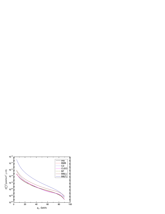
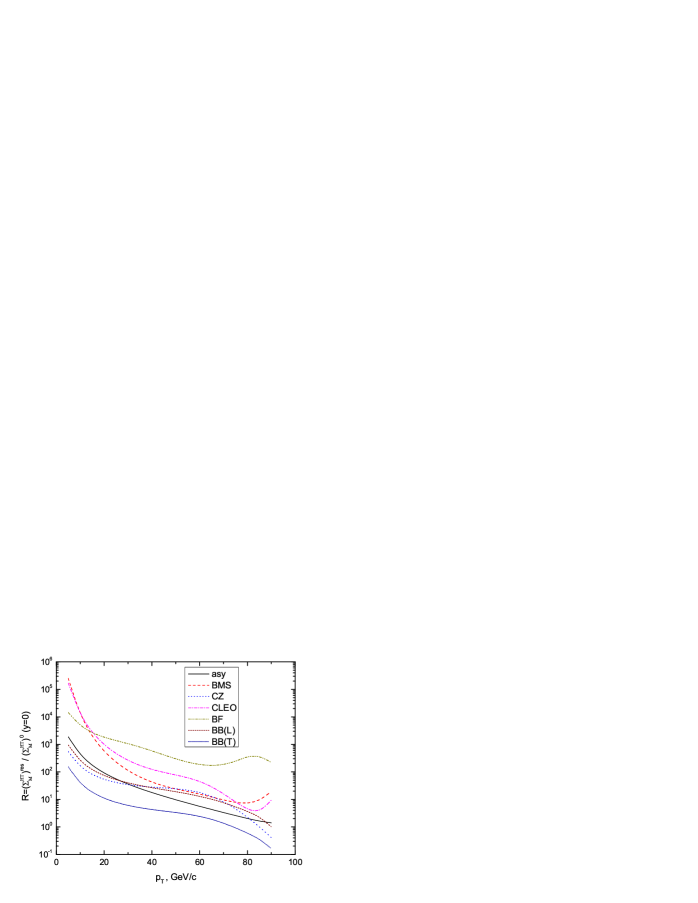
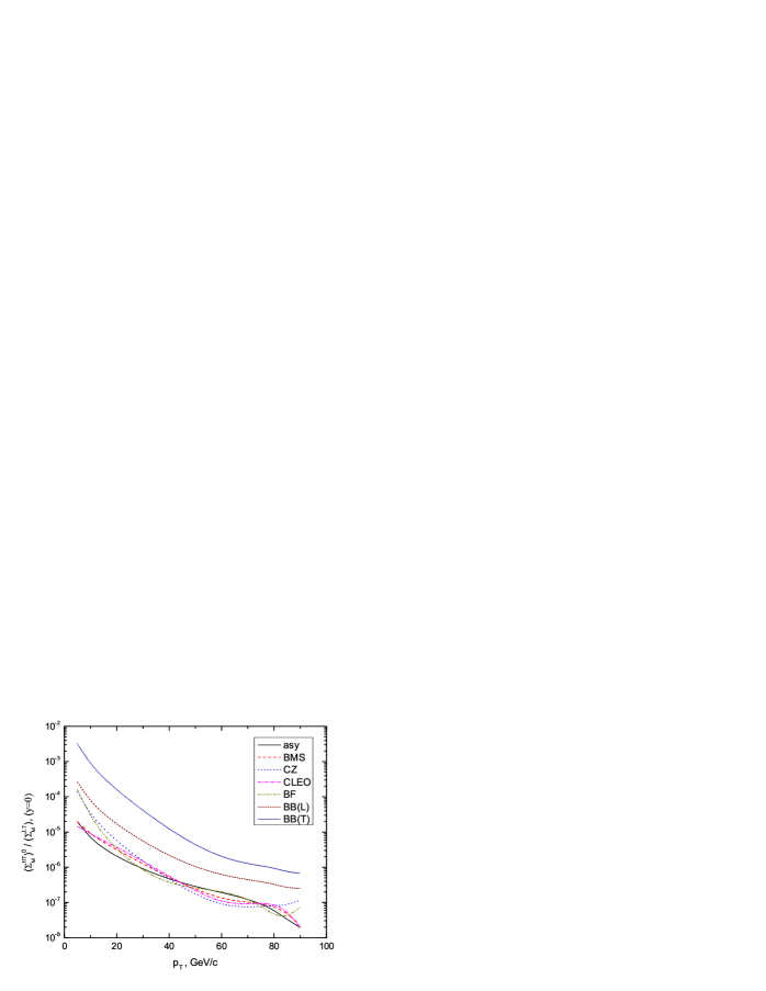
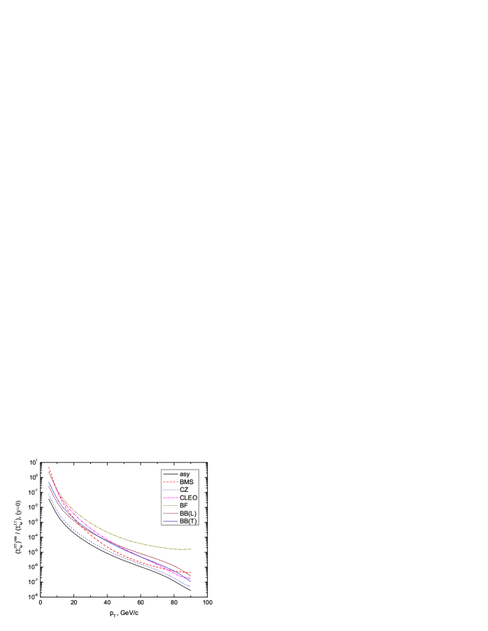
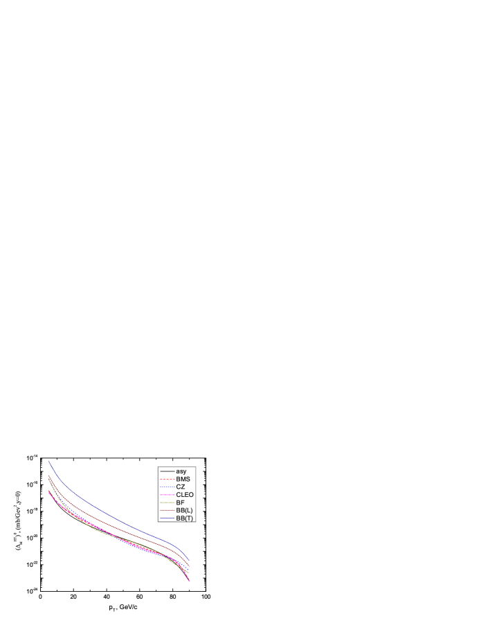
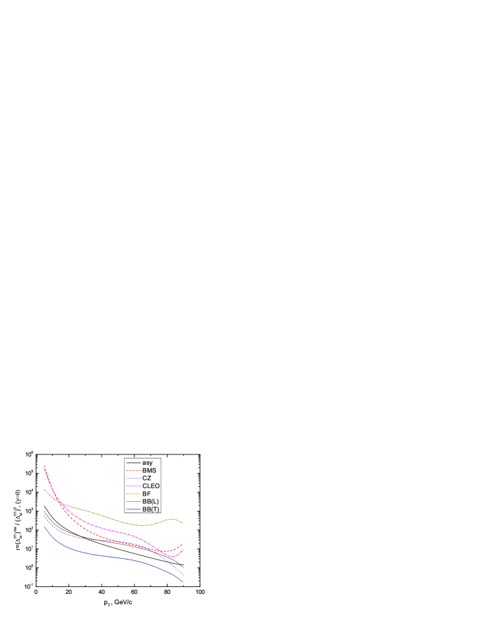
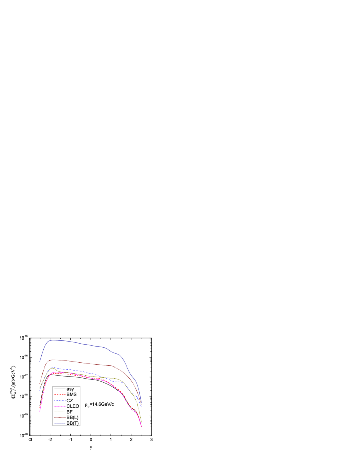
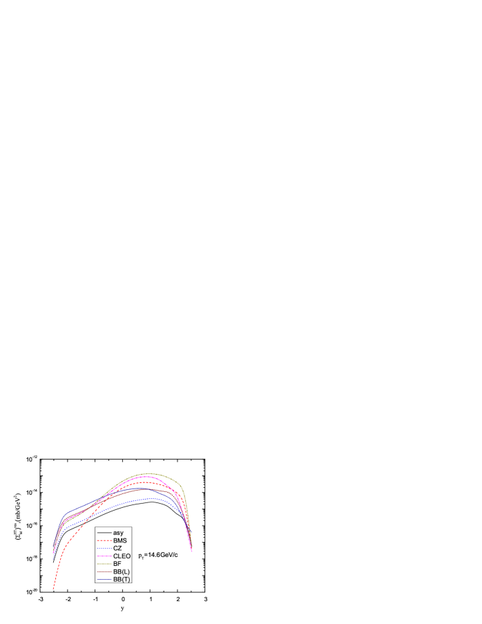
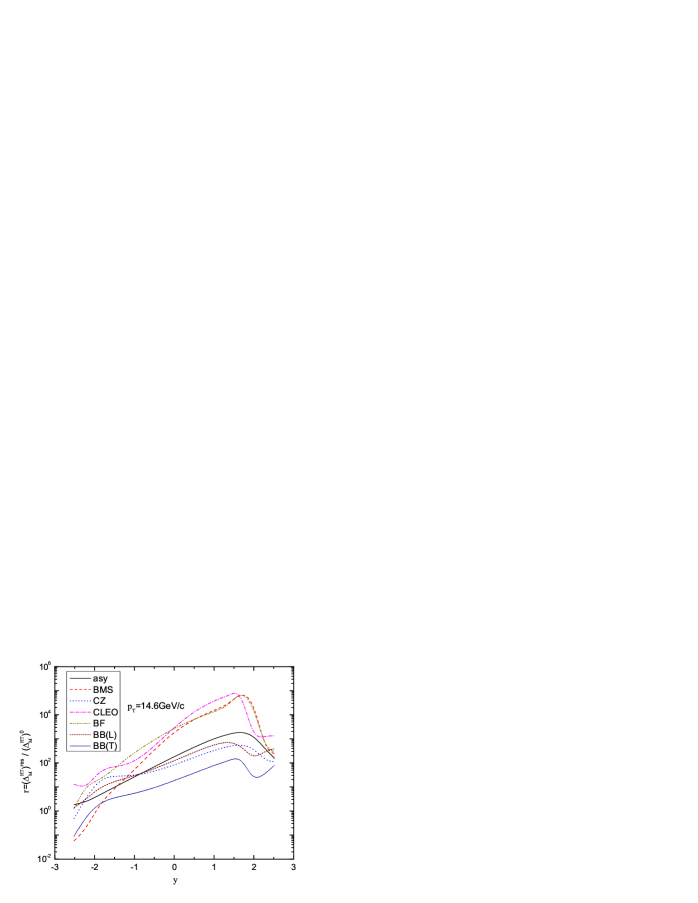
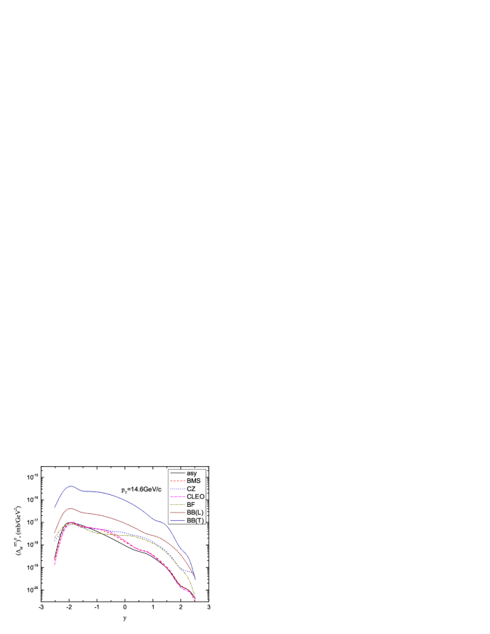
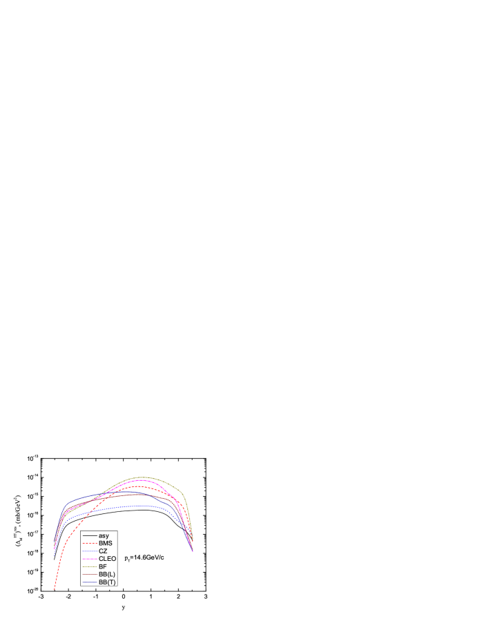
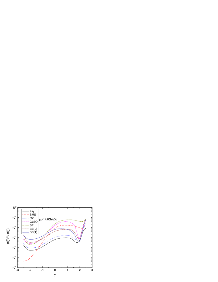
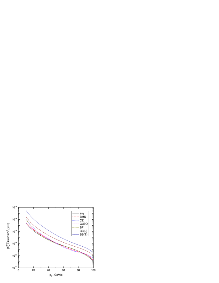
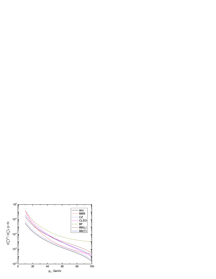
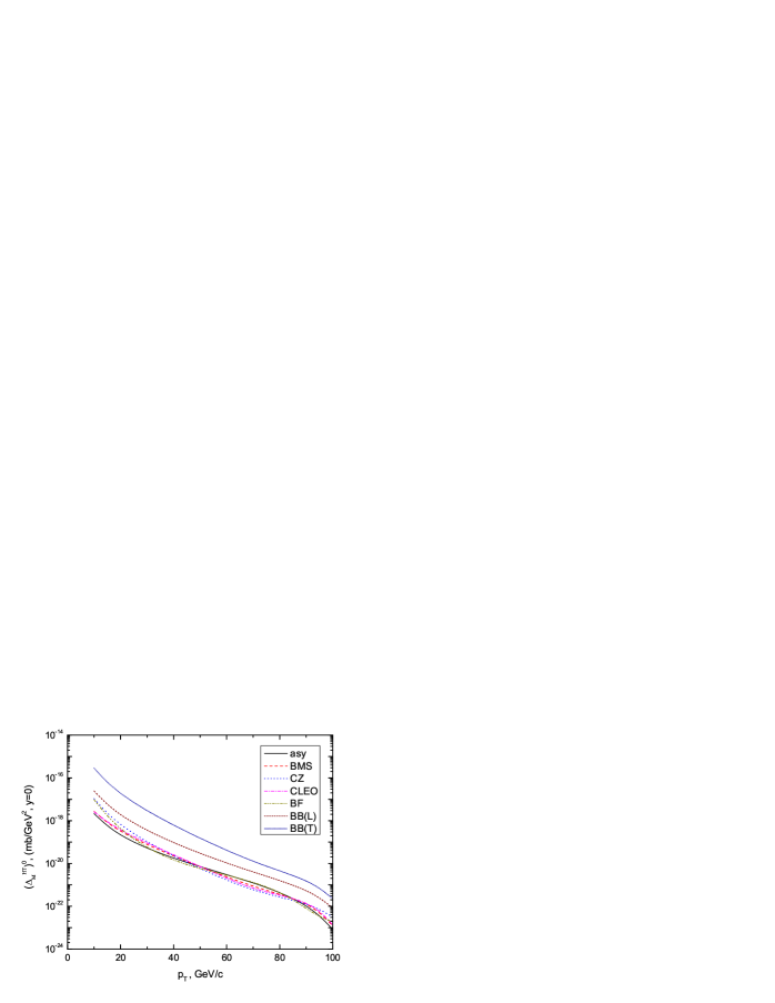
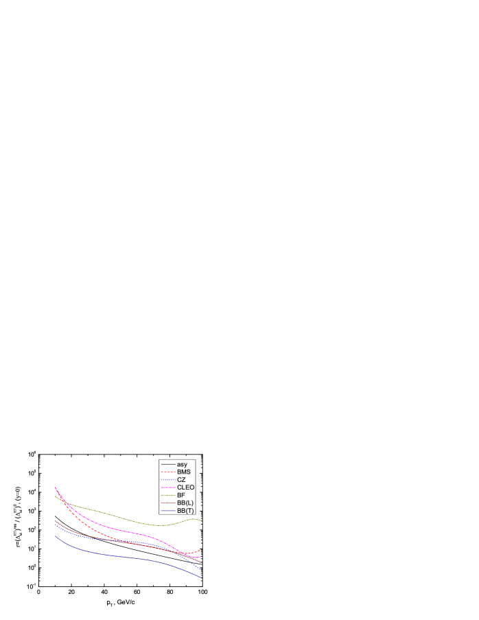
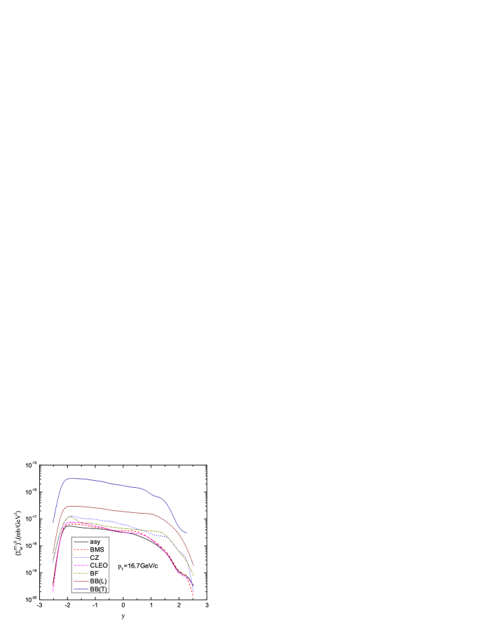
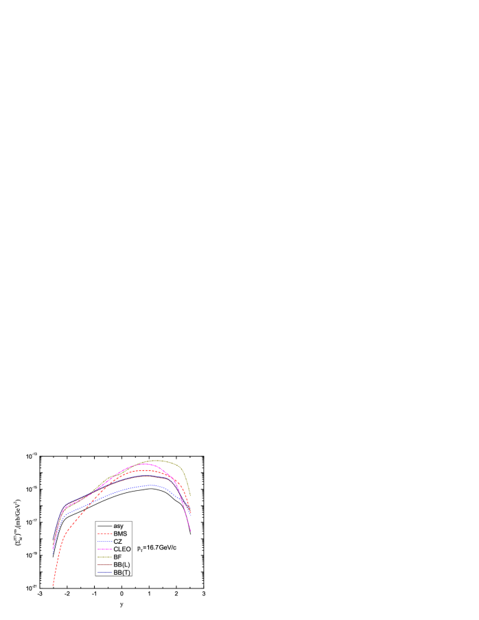
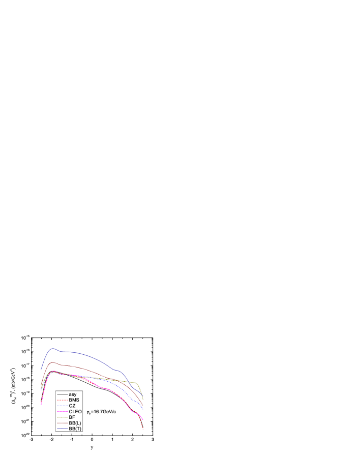
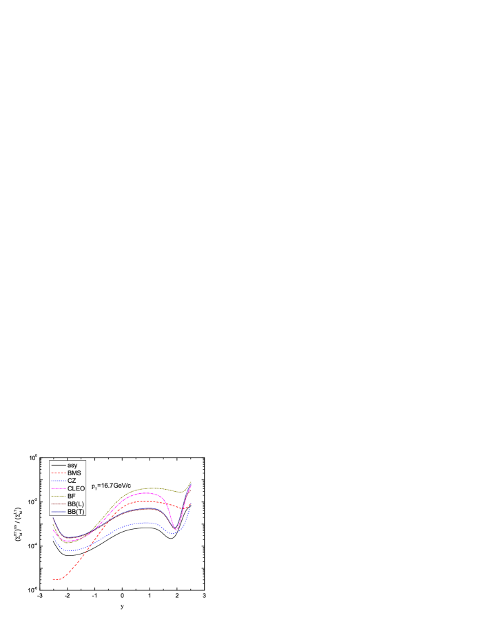
In this section, we discuss the numerical results for higher-twist effects with higher-twist contributions calculated in the context of the running coupling constant and frozen coupling approaches on the dependence of the chosen meson wave functions in the process $\gamma\gamma\to MX$. We have calculated the dependence on the meson wave functions for the higher-twist contribution to the large-$p_{T}$ single pseudoscalar ${\pi^{+}}$ and vector $\rho_{L}^{+}$, $\rho_{T}^{+}$ mesons production cross section in the photon-photon collision. The ${\pi^{-}}$, ${\rho_{L}^{-}}$, ${\rho_{T}^{-}}$ cross sections are, of course, identical. In the calculations, we use the asymptotic wave function $\Phi_{asy}$, the Chernyak-Zhitnitsky $\Phi_{CZ}$, the pion wave function from which two nontrivial Gegenbauer coefficients $a_{2}$ and $a_{4}$ have been extracted from the CLEO data on the $\pi^{0}\gamma$ transition form factor[46], the Braun-Filyanov pion wave functions [11], and the Bakulev-Mikhailov-Stefanis pion wave function[ 47]. For $\rho$-meson we used Ball-Braun wave function[51]. For the higher-twist subprocess, we take $\gamma q_{1}\to(q_{1}\overline{q}_{2})q_{2}$, $\gamma\overline{q}_{2}\to(q_{1}\overline{q}_{2})\overline{q}_{2}$ contributing to $\gamma\gamma\to MX$ cross sections. Inclusive meson photoproduction represents a significant test case in which higher-twist terms dominate those of leading-twist in certain kinematic domains. For the dominant leading-twist subprocess for the meson production, we take the photon-photon annihilation $\gamma\gamma\to q\bar{q}$, in which the $M$ meson is indirectly emitted from the quark. For example, the quark distribution function inside the photon has been used [56]. The higher-twist subprocesses probe the meson wave functions over a large range of $Q^{2}$ squared momentum transfer, carried by the gluon. Therefore, in the diagram given in Fig.1a we take $Q_{1}^{2}=x_{2}{\hat{s}}$, $Q_{2}^{2}=-x_{1}\hat{u}$ , which we have obtained directly from the higher-twist subprocesses diagrams. The same $Q_{1,2}^{2}$ has been used as an argument of $\alpha_{s}(Q_{1,2}^{2})$ in the calculation of diagram.

The results of our numerical calculations are plotted in Figs.2-33. First of all, it is very interesting to compare the resummed higher-twist cross sections with the ones obtained in the framework of the frozen coupling approach. In Figs.2-4 we show the dependence of higher-twist cross sections $(\Sigma_{M^{+}}^{HT})^{0}$ calculated in the context of the frozen coupling, $(\Sigma_{M^{+}}^{HT})^{res}$ in the context of the running coupling constant approaches and also the ratio $R=(\Sigma_{M^{+}}^{HT})^{res}$/$\Sigma_{M^{+}}^{HT})^{0}$ as a function of the meson transverse momentum $p_{T}$ for different meson wave functions at $y=0$. It is seen that the values of cross sections $(\Sigma_{M^{+}}^{HT})^{0}$, $(\Sigma_{M^{+}}^{HT})^{res}$, and $R$ for fixed $y$ and $\sqrt{s}$ depend on the choice of the meson wave function. As seen from Figs.2-3 in both cases, frozen coupling and running coupling constant approaches the higher-twist differential cross section is monotically decreasing with an increase in the transverse momentum of the meson. As is seen from Fig.4, when the transverse momentum of the meson is increasing, the ratio $R$ is decreasing. But, as shown in Fig.4, in the region $5\,\,GeV/c<p_{T}<80\,\,GeV/c$ higher-twist cross section calculated in the context of the running coupling method is suppressed by about 2-4 orders of magnitude relative to the higher-twist cross section calculated in the framework of the frozen coupling method. In Figs.5 and 6, we shows the dependence of the ratio $(\Sigma_{M^{+}}^{HT})^{0}$/$(\Sigma_{M^{+}}^{LT})$ and $(\Sigma_{M^{+}}^{HT})^{res}$/$(\Sigma_{M^{+}}^{LT})$ as a function of the meson transverse momentum $p_{T}$ for different meson wave functions. Here $(\Sigma_{M^{+}}^{LT})$ is the leading-twist cross section, respectively. As seen from Fig.6, in the region $5\,\,GeV/c<p_{T}<10\,\,GeV/c$ higher-twist cross section for $\Phi_{BMS}(x,Q^{2}))$ and $\Phi_{CLEO}(x,Q^{2}))$ wave functions calculated in the context of the running coupling method is suppressed by about one orders of magnitude relative to the leading-twist cross section, but in the region $10\,\,GeV/c<p_{T}\leq 90\,\,GeV/c$ ratio is decreasing with an increase in the transverse momentum of the meson. In Figs.7-9 we show the dependence $(\Delta_{M}^{HT})^{0}$, $(\Delta_{M}^{HT})^{res}$, and the ratio $r$=($\Delta_{M}^{HT})^{res}$/$(\Delta_{M}^{HT})^{0}$, as a function of the meson transverse momentum $p_{T}$ for the different meson wave functions. Here, $(\Delta_{M}^{HT})^{0}=(\Sigma_{M^{+}}^{HT})^{0}-(\Sigma_{M^{-}}^{HT})^{0}$ and $(\Delta_{M}^{HT})^{res}=(\Sigma_{M^{+}}^{HT})^{res}-(\Sigma_{M^{-}}^{HT})^{res}$. As seen from Figs.7 and 8, the difference of the higher-twist differential cross section is decreasing with an increase in the transverse momentum of the meson. The dependence, as shown in Fig.9, is identically equivalent to Fig.4. In Figs.10-17, we have depicted higher-twist cross sections, ratios $(\Sigma_{M^{+}}^{HT})^{0}$, $(\Sigma_{M^{+}}^{HT})^{res}$, $R=(\Sigma_{M^{+}}^{HT})^{res}$/$(\Sigma_{M^{+}}^{HT})^{0}$, $r$=($\Delta_{M}^{HT})^{res}$/$(\Delta_{M}^{HT})^{0}$, $(\Delta_{M}^{HT})^{0}$, $(\Delta_{M}^{HT})^{res}$, $(\Sigma_{M^{+}}^{HT})^{0}$/$(\Sigma_{M^{+}}^{LT})$ and $(\Sigma_{M^{+}}^{HT})^{res}$/$(\Sigma_{M^{+}}^{LT})$ as a function of the rapidity $y$ of the meson at $\sqrt{s}=183\,\,GeV$ and $p_{T}=14.6\,\,GeV/c$. At $\sqrt{s}=183\,\,GeV$ and $p_{T}=14.6\,\,GeV/c$, the meson rapidity lies in the region $-2.52\leq y\leq 2.52$.

As seen from Fig.10 and Fig.14, in the region ($-2.52\leq y\leq-1.92$), the cross section for all wave functions increases with an increase of the $y$ rapidity of the meson and have a maximum approximately at the point $y=-1.92$. Besides that, the cross sections decrease with an increase in the $y$ rapidity of the meson. But, as seen from Figs.12 and 13 in the region ($-2.52\leq y\leq 1.92$) the cross section for all wave functions increases with an increase of the $y$ rapidity of the meson and has a maximum approximately at the point $y=1.92$. But, as seen from Figs.16-17 in the region ($-2.52\leq y\leq 1.92$) the cross section for all wave functions has a minimum approximately at the point $y=1.92$. As is seen from Figs.10-17, cross sections, the ratios $R$ and $r$ are very sensitive to the choice of the meson wave functions. It should be noted that the magnitude of the higher-twist cross section for the pion wave functions $\Phi_{BMS}(x,Q^{2})$ and $\Phi_{CLEO}(x,Q^{2})$ is very close to the asymptotic wave function $\Phi_{asy}(x)$. Also, the distinction between $R(\Phi_{asy}(x))$ with $R(\Phi_{BMS}(x,Q^{2}))$, $R(\Phi_{CZ}(x,Q^{2}))$, $R(\Phi_{CLEO}(x,Q^{2}))$, $R(\Phi_{BF}(x,Q^{2}))$, $R(\Phi_{BB(L)}(x,Q^{2}))$ and $R(\Phi_{BB(T)}(x,Q^{2}))$ have been calculated. For example, in the case of $\sqrt{s}=183\,\,GeV$, $y=0$, the distinction between $R(\Phi_{asy}(x))$ with $R(\Phi_{i}(x,Q^{2}))$  [i=BMS, CZ, CLEO, BF, BB(L), BB(T)] as a function of the meson transverse momentum $p_{T}$ is shown in Table 1. Thus, the distinction between $R(\Phi_{asy}(x))$ with $R(\Phi_{i}(x,Q^{2}))$,  [i=BMS, CLEO] is maximum at $p_{T}=5\,\,GeV/c$, with $R(\Phi_{CZ}(x))$ at $p_{T}=50\,\,GeV/c$; the distinction between $R(\Phi_{asy}(x))$ with $R(\Phi_{BF}(x,Q^{2}))$, is maximum at $p_{T}=90\,\,GeV/c$; but the distinction $R(\Phi_{asy}(x))$ with $R(\Phi_{i}(x,Q^{2}))$,  [i=BB(L), BB(T)] is maximum at $p_{T}=75\,\,GeV/c$, Also, we have calculated the distinction between $R(\Phi_{asy}(x))$ with $R(\Phi_{i}(x,Q^{2}))$  [i=BMS, CZ, CLEO, BF, BB(L), BB(T)] as a function of the rapidity $y$ of the meson. For example, in the case of $\sqrt{s}=183GeV$, $p_{T}=14.6GeV/c$ the distinction between $R(\Phi_{asy}(x))$ with $R(\Phi_{i}(x,Q^{2}))$   [i=BMS, CZ, CLEO, BF, BB(L), BB(T)] as a function of the rapidity $y$ of the meson is presented in Table 2

We have also carried out comparative calculations in the center-of-mass energy $\sqrt{s}=209\,\,GeV$. The results of our numerical calculations in the center-of-mass energies $\sqrt{s}=209\,\,GeV$ are plotted in Figs.18-33. Analysis of our calculations at the center-of-mass energies $\sqrt{s}=183\,\,GeV$ and $\sqrt{s}=209\,\,GeV$, show that with the increase in beam energy values of the cross sections, ratio $R=(\Sigma_{M^{+}}^{HT})^{res}/(\Sigma_{M^{+}}^{HT})^{0}$, and contributions of higher-twist to the cross section decrease by about 1-2 order. Therefore the experimental investigation of higher-twist effects include renormalon effects conveniently in low energy. On the other hand, the higher-twist corrections and ratios $R$ and $r$ are very sensitive to the choice of the meson wave function. Also, the distinction between $R(\Phi_{asy}(x))$ with $R(\Phi_{BMS}(x,Q^{2}))$, $R(\Phi_{CZ}(x,Q^{2}))$, $R(\Phi_{CLEO}(x,Q^{2}))$, $R(\Phi_{BF}(x,Q^{2}))$, $R(\Phi_{BB(L)}(x,Q^{2}))$ and $R(\Phi_{BB(T)}(x,Q^{2}))$ have been calculated. For example, in the case of $\sqrt{s}=209\,\,GeV$, $y=0$, the distinction between $R(\Phi_{asy}(x))$ with $R(\Phi_{i}(x,Q^{2}))$  [i=BMS, CZ, CLEO, BF, BB(L), BB(T)] as a function of the meson transverse momentum $p_{T}$ is shown in Table 3. Thus, the distinction between $R(\Phi_{asy}(x))$ with $R(\Phi_{i}(x,Q^{2}))$,  (i=BMS, CLEO) is maximum at $p_{T}=10\,\,GeV/c$, with $R(\Phi_{CZ}(x))$ at $p_{T}=65\,\,GeV/c$; the distinction between $R(\Phi_{asy}(x))$ with $R(\Phi_{BF}(x,Q^{2}))$, is maximum at $p_{T}=100\,\,GeV/c$; but the distinction $R(\Phi_{asy}(x))$ with $R(\Phi_{i}(x,Q^{2}))$,  (i=BB(L), BB(T)) is maximum at $p_{T}=65\,\,GeV/c$. Also, we have calculated the distinction between $R(\Phi_{asy}(x))$ with $R(\Phi_{i}(x,Q^{2}))$  [i=BMS, CZ, CLEO, BF, BB(L), BB(T)] as a function of the rapidity $y$ of the meson. For example, in the case of $\sqrt{s}=209GeV$, $p_{T}=16.7GeV/c$ the distinction between $R(\Phi_{asy}(x))$ with $R(\Phi_{i}(x,Q^{2}))$   [i=BMS, CZ, CLEO, BF, BB(L), BB(T)] as a function of the rapidity $y$ of the meson is presented in Table 4. The calculations show that the ratio $R(\Phi_{i}(x,Q^{2}))$/$R(\Phi_{asy}(x))$, (i=CLEO, CZ, BF, BMS, BB(L), BB(T)) for all values of the transverse momentum $p_{T}$ of the meson identically equivalent to ratio $r(\Phi_{i}(x,Q^{2}))$/$r(\Phi_{asy}(x))$. Results of our numerical calculations demonstrate that in the renormalon approach there are not difference between results obtained using the cross sections (2.13), (2.14) or (2.11), (2.12).

The total integrated luminosity of LEP is 612.8$pb^{-1}$ and total luminosity of ILC required is 500$fb^{-1}$, also a peak luminosity of ILC is 1000 $fb^{-1}$ during the first phase of operation at $209GeV\div 500GeV$. In our calculations of the higher-twist cross section of the process the dependence of the transverse momentum of meson appears in the range of $(10^{-10}\div 10^{-24})mb/GeV^{2}$, or $(10^{-1}\div 10^{-15})pb/GeV^{2}$. Therefore, higher-twist cross section obtained in our paper should be observable at LEP and ILC.

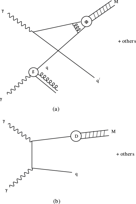
VI Concluding Remarks

In this work we have calculated the single meson inclusive production via higher-twist mechanism and obtained the expressions for the subprocess $\gamma q\to Mq$ cross section for mesons with symmetric wave functions. For calculation of the cross section we have applied the running coupling constant method and revealed infrared renormalon poles in the cross section expression. Infrared renormalon induced divergences have been regularized by means of the principal value prescription and the resummed expression (the Borel sum) for the higher-twist cross section has been found. The higher-twist cross sections were calculated in the frozen coupling and running coupling approaches. The resummed higher-twist cross section differs from that found using the frozen coupling approach, in some regions, considerably. Also we demonstrated that higher-twist contributions to single meson production cross section in the photon-photon collisions have important phenomenological consequences. We have obtained very interesting results. The ratio $R$ for all values of the transverse momentum $p_{T}$ and of the rapidity $y$ of the meson identically equivalent to ratio $r$. Our investigation enables us to conclude that the higher-twist meson production cross section in the photon-photon collisions depends on the form of the meson model wave functions and may be used for their study. Analysis of our calculations shows that the magnitude of cross sections of the leading-twist is larger than the higher-twist cross sections ones calculated in the frozen coupling approach in 2-4 order. But, in some regions of transverse momentum of the meson, the higher-twist cross section calculated in the context of the running coupling method is comparable with the cross sections of leading-twist. Further investigations are needed in order to clarify the role of high twist effects in this process. We have demonstrated that the resummed result depends on the meson model wave functions used in calculations. The production of high-$p_{T}$ meson probes the short-distance dynamics of photon-photon reactions. In addition to providing tests of perturbative QCD, $\gamma\gamma$ processes with real or almost real photons give us information on the photon structure function which is complementary to the information gained from deep inelastic scattering on a real photon. The latter process essentially probes the quark distribution while high-$p_{T}$ meson production is also sensitive to the gluon distribution of the photon. As it is well known high-$p_{T}$ processes induced by real photons have a rather complex structure. This arises from the fact that the photon couples to the hard subprocess either directly or through its quark and gluon content. In particular, meson production in photon-photon collisions takes into account infrared renormalon effects: this opens a window toward new types of photon structure function which can not be measured by the lepton-photon scatterings.

VII References

G. P. Lepage and S. J.  Brodsky, Phys. Lett. 87B, 359 (1979); Phys. Rev. Lett. 43, 545 (1979); 43, 1625(E) (1979);

G. P. Lepage and S. J. Brodsky, Phys. Rev. D22, 2157 (1980).

A. V. Efremov and A. V. Radyushkin, Theor. Mat. Phys. 42, 97 (1980); Phys. Lett. 94B, 245 (1980).

A. Duncan and A. Mueller, Phys. Lett. 90B, 159 (1980); Phys. Rev. D21, 1636 (1980).

A.V. Radyushkin, Dubna Report No. P2-10717, 1977.

V. L. Chernyak and A. R. Zhitnitsky, Nucl. Phys. B201, 492 (1982).

V. L. Chernyak and A. R. Zhitnitsky, Nucl. Phys. B246, 52 (1984).

I. D. King, C. T. Sachrajda, Nucl. Phys. B279, 785 (1987).

V. L. Chernyak, A. R. Zhitnitsky, Phys. Rep. 112, 173 (1984).

S. V. Mikhailov and A. V. Radyushkin, Pis’ma Zh. Eksp. Teor. Fiz. 43, 551 (1986)[JETP Lett. 43, 712 (1986)]; Yad. Fiz. 49, 794 (1988)[Sov. J. Nucl. Phys. 49, 494 (1989)]; Phys. Rev. D45, 1754 (1992).

V. M. Braun and I. E. Filyanov, Z. Phys. C44, 157 (1989).

G. R. Farrar, K. Huleihel and H. Zhang, Nucl. Phys. B349, 655 (1991).

A. V. Radyushkin and R. Ruskov, Phys. Lett. B374, 173 (1996); Nucl. Phys. B481, 625 (1996).

S. J. Brodsky and G. L. Lepage, in Perturbative Quantum Chromodynamics, edited by A. H. Mueller, (World Scientific, Singapore, 1989), p.93.

S. J. Brodsky, H.-C.Pauli and S. S. Pinsky, Phys. Rep. 301, 299 (1998).

J. Gronberg $et.al.$ (The CLEO Collaboration), Phys. Rev. D57, 33 (1998).

V. Yu. Petrov, M. V. Polyakov, R. Ruskov, C. Weiss and K. Goeke, Phys. Rev. D59, 114018 (1999); hep-ph/9807229.

S. V. Mikhailov, J.High Energy Phys. 06 (2007) 009.

V. A. Matveev, R. M. Muradyan, and A. N. Tavkhelidze, Lett. Nuovo Cimento 7, 719 (1973).

S. J. Brodsky and G.R. Farrar, Phys. Rev. Lett. 31, 1153 (1973).

J. F. Gunion, S. J. Brodsky, and R. Blankenbacler,Phys. Rev. D6, 2652 (1972).

V. A. Matveev, L. A. Slepchenko, and A. N. Tavkhelidze, Phys. Lett. 100B, 75 (1981).

J. A. Bagger and J. F. Gunion, Phys. Rev. D25, 2287 (1982).

V. N. Baier and A. G. Grozin, Phys. Lett. 96B, 181 (1980).

S. J. Brodsky, G. P. Lepage and P. B. Mackenzie, Phys. Rev. D28, 228 (1983).

A. I. Ahmadov, I. Boztosun, A. Soylu and E. A. Dadashov, Int. J. Mod. Phys. E17, 1041 (2008); hep-ph/0611365.

M. Maul, E. Stein, A. Schafer, and L. Mankiewich, Phys. Lett. B401, 100 (1997).

Y. L. Dokshitzer, V. A. Khoze and S. I. Troyan, Phys. Rev. D53, 89 (1996).

A. L. Kataev, Mod. Phys. Lett. A 20, 2007 (2005).

G.’t Hooft, in The Whys of Subnuclear Physics, Erice, 1977, edited by A. Zichnichi(Plenum, New York, 1979), p.94.

H. Contopanagos and G. Sterman, Nucl. Phys. B419, 77 (1994).

W. Greiner, S. Schramm, and E. Stein, Quantum Chromodynamics (Springer,Berlin,2002), 2nd ed., p.551.

D. V. Shirkov and I. L. Solovtsov, Phys. Rev. Lett. 79, 1209 (1997).

J.  Botts and G.  Sterman, Nucl.Phys. B325, 62 (1989).

I. V.  Anikin, D. Yu.  Ivanov, B. Pire, L. Szymanowski, and S. Wallon, Nucl. Phys. B828, 1 (2010); Phys. Lett. B682, 413 (2010).

E. Gardi, G. Grunberg and M. Karliner, J. High Energy Phys. 07 (1998) 007.

S. S. Agaev, Phys. Lett. B360, 117 (1995); B369, 379(E) (1996); Mod. Phys. Lett. A10, 2009 (1995);11, 957 (1996)

A. I. Ahmadov, Coskun  Aydin, Sh. M. Nagiyev, Yilmaz A. Hakan, and E. A. Dadashov, Phys. Rev. D80, 016003 (2009).

V. M. Budnev, I. F. Ginzburg, G. V. Meledin, and V. G. Serbo, Phys. Rep. 15, 181 (1975).

J. A. Bagger and J. F. Gunion, Phys. Rev. D29, 40 (1984).

J. A. Bagger and J. F. Gunion, Phys. Rev. D25, 2287 (1982).

J. A. Hassan and J. K. Storrow, Z. Phys. C14, 65 (1982).

S. J. Brodsky, T. A. DeGrand, J. F. Gunion and J. H. Weis, Phys. Rev. Lett 41, 672 (1978); Phys. Rev. D19, 1418 (1979).

G. P. Lepage and S. J.  Brodsky, Phys. Lett. 87B, 359 (1979); Phys. Rev. Lett. 43, 545 (1979); 43, 1625(E) (1979); A. Duncan and A. Mueller, Phys. Rev. D21, 1636 (1980).

G. P. Lepage and S. J. Brodsky, Phys. Rev. D22, 2157 (1980).

A. Schmedding and O. Yakovlev, Phys. Rev. D62, 116002 (2000).

A. P. Bakulev, S. V. Mikhailov and N. G. Stefanis, Phys. Lett, B578, 91 (2004).

S. V. Mikhailov and A. V. Radyushkin, Phys. Rev. D45, 1754 (1992).

A. P. Bakulev, S. V. Mikhailov, Z. Phys. C68, 451 (1995).

A. E. Dorokhov, JETP Lett. 77, 63 (2003).

P. Ball and V. M. Braun, Phys. Rev. D54, 2182 (1996); hep-ph/9602323.

S. S. Agaev, Eur. Phys. J. C 1, 321 (1998).

M. Beneke and V. M. Braun, Phys. Lett. B348, 513 (1995); P. Ball, M. Beneke and V. M. Braun, Nucl. Phys. B452, 563 (1995); M. Beneke, Nucl. Phys. B405, 424 (1993).

J. Zinn-Justin, Phys. Rep. 70, 109 (1981).

A. Erdelyi, Higher Transcendental Functions (McGrow-Hill, New York, 1953), Vol.2.

F. Cornet, Acta Phys. Polon. B37, 663 (2006); hep-ph/0601056.

$p_{T},GeV/c$	$\frac{R(\Phi_{BMS}(x,Q^{2}))}{R(\Phi_{asy}(x))}$	$\frac{R(\Phi_{CZ}(x,Q^{2}))}{R(\Phi_{asy}(x))}$	$\frac{R(\Phi_{CLEO}(x,Q^{2}))}{R(\Phi_{asy}(x))}$	$\frac{R(\Phi_{BF}(x,Q^{2}))}{R(\Phi_{asy}(x))}$	$\frac{R(\Phi_{BB(L)}(x,Q^{2}))}{R(\Phi_{asy}(x))}$	$\frac{R(\Phi_{BB(T)}(x,Q^{2}))}{R(\Phi_{asy}(x))}$
5	132.678	0.288	89.019	7.621	0.499	0.0808
30	3.064	0.949	7.24	29.651	1.103	0.167
50	2.46	2.516	7.955	30.635	1.962	0.343
75	2.992	1.778	3.12	92.936	2.091	0.359
90	13.888	0.293	6.744	157.748	0.712	0.116

Table 1: The distinction between $R(\Phi_{asy}(x))$ with $R(\Phi_{i}(x,Q^{2}))$ (i=BMS, CZ, CLEO, BF, BB(L), BB(T) ) at c.m. energy $\sqrt{s}=183GeV$.

$y$	$\frac{R(\Phi_{BMS}(x,Q^{2}))}{R(\Phi_{asy}(x))}$	$\frac{R(\Phi_{CZ}(x,Q^{2}))}{R(\Phi_{asy}(x))}$	$\frac{R(\Phi_{CLEO}(x,Q^{2}))}{R(\Phi_{asy}(x))}$	$\frac{R(\Phi_{BF}(x,Q^{2}))}{R(\Phi_{asy}(x))}$	$\frac{R(\Phi_{BB(L)}(x,Q^{2}))}{R(\Phi_{asy}(x))}$	$\frac{R(\Phi_{BB(T)}(x,Q^{2}))}{R(\Phi_{asy}(x))}$
-2.52	0.0307	0.259	7.091	0.6706	0.751	0.048
-1.92	0.338	4.052	9.741	4.327	1.965	0.448
0.78	14.858	0.344	34.922	13.642	0.586	0.0794
1.38	18.125	0.309	40.788	15.9209	0.477	0.0792
2.28	0.9125	0.327	3.3298	1.0724	0.8047	0.0895

Table 2: The distinction between $R(\Phi_{asy}(x))$ with $R(\Phi_{i}(x,Q^{2}))$ (i=BMS, CZ, CLEO, BF, BB(L), BB(T)) at c.m. energy $\sqrt{s}=183GeV$.

$p_{T},GeV/c$	$\frac{R(\Phi_{BMS}(x,Q^{2}))}{R(\Phi_{asy}(x))}$	$\frac{R(\Phi_{CZ}(x,Q^{2}))}{R(\Phi_{asy}(x))}$	$\frac{R(\Phi_{CLEO}(x,Q^{2}))}{R(\Phi_{asy}(x))}$	$\frac{R(\Phi_{BF}(x,Q^{2}))}{R(\Phi_{asy}(x))}$	$\frac{R(\Phi_{BB(L)}(x,Q^{2}))}{R(\Phi_{asy}(x))}$	$\frac{R(\Phi_{BB(T)}(x,Q^{2}))}{R(\Phi_{asy}(x))}$
10	33.874	0.352	33.404	11.184	0.568	0.08812
35	2.537	0.9789	6.7409	29.866	1.1213	0.1704
65	2.167	3.0311	7.7455	30.915	2.2177	0.4091
85	2.358	1.841	3.0529	86.0547	2.0994	0.3638
100	6.5605	0.4398	3.0772	194.339	1.1648	0.1833

Table 3: The distinction between $R(\Phi_{asy}(x))$ with $R(\Phi_{i}(x,Q^{2}))$ (i=BMS, CZ, CLEO, BF, BB(L), BB(T)) at c.m. energy $\sqrt{s}=209GeV$.

$y$	$\frac{R(\Phi_{BMS}(x,Q^{2}))}{R(\Phi_{asy}(x))}$	$\frac{R(\Phi_{CZ}(x,Q^{2}))}{R(\Phi_{asy}(x))}$	$\frac{R(\Phi_{CLEO}(x,Q^{2}))}{R(\Phi_{asy}(x))}$	$\frac{R(\Phi_{BF}(x,Q^{2}))}{R(\Phi_{asy}(x))}$	$\frac{R(\Phi_{BB(L)}(x,Q^{2}))}{R(\Phi_{asy}(x))}$	$\frac{R(\Phi_{BB(T)}(x,Q^{2}))}{R(\Phi_{asy}(x))}$
-2.25	0.0223	0.2596	6.0611	0.7024	0.7847	0.0639
-1.92	0.2747	3.8857	8.6517	4.122	1.9435	0.2391
0.78	12.9913	0.3491	32.4146	7.0045	0.5867	0.07707
1.38	15.879	0.3138	37.443	2.7794	0.475	0.1251
2.28	0.7783	0.3323	2.9838	0.4545	0.8104	0.2131

Table 4: The distinction between $R(\Phi_{asy}(x))$ with $R(\Phi_{i}(x,Q^{2}))$ (i=BMS, CZ, CLEO, BF, BB(L), BB(T)) at c.m. energy $\sqrt{s}=209GeV$.

Figure 1: (a): The higher-twist contribution to $\gamma\gamma\to MX$;   (b): The leading-twist contribution to $\gamma\gamma\to MX$

Figure 2: Higher-twist $M$ production cross section $(\Sigma^{HT})^{0}$ as a function of the $p_{T}$ transverse momentum of the meson at the c.m.energy $\sqrt{s}=183\,\,GeV$.

Figure 3: Higher-twist $M$ production cross section $(\Sigma^{HT})^{res}$ as a function of the $p_{T}$ transverse momentum of the meson at the c.m.energy $\sqrt{s}=183\,\,GeV$.

Figure 4: Ratio $R=(\Sigma_{M}^{HT})^{res}/(\Sigma_{M}^{HT})^{0}$, where higher-twist contribution are calculated for the meson rapidity $y=0$ at the c.m.energy $\sqrt{s}=183\,\,GeV$ as a function of the meson transverse momentum, $p_{T}$.

Figure 5: Ratio $(\Sigma_{M}^{HT})^{0}/(\Sigma_{M}^{LT})$, as a function of the $p_{T}$ transverse momentum of the meson at the c.m. energy $\sqrt{s}=183\,\,GeV$.

Figure 6: Ratio $(\Sigma_{M}^{HT})^{res}/(\Sigma_{M}^{LT})$, as a function of the $p_{T}$ transverse momentum of the meson at the c.m. energy $\sqrt{s}=183\,\,GeV$.

Figure 7: The difference of the higher-twist cross section, $(\Delta_{M}^{HT})^{0}=(\Sigma_{M^{+}}^{HT})^{0}-(\Sigma_{M^{-}}^{HT})^{0}$, as a function of the meson transverse momentum, $p_{T}$, at the c.m.energy $\sqrt{s}=183\,\,GeV$.

Figure 8: The difference of the higher-twist cross section, $(\Delta_{M}^{HT})^{res}=(\Sigma_{M^{+}}^{HT})^{res}-(\Sigma_{M^{-}}^{HT})^{res}$, as a function of the meson transverse momentum, $p_{T}$, at the c.m.energy $\sqrt{s}=183\,\,GeV$.

Figure 9: Ratio $r=(\Delta_{M}^{HT})^{res}/(\Delta_{M}^{HT})^{0}$, where higher-twist contributions are calculated for the meson rapidity $y=0$ at the c.m. energy $\sqrt{s}=183\,\,GeV$, as a function of the meson transverse momentum, $p_{T}$.

Figure 10: Higher-twist $M$ production cross section $(\Sigma_{M}^{HT})^{0}$, as a function of the $y$ rapidity of the meson at the transverse momentum of the meson $p_{T}=14.6\,\,GeV/c$, at the c.m. energy $\sqrt{s}=183\,\,GeV$.

Figure 11: Higher-twist $M$ production cross section $(\Sigma_{M}^{HT})^{res}$, as a function of the $y$ rapidity of the meson at the transverse momentum of the meson $p_{T}=14.6\,\,GeV/c$, at the c.m. energy $\sqrt{s}=183\,\,GeV$.

Figure 12: Ratio $R=(\Sigma_{M}^{HT})^{res}/(\Sigma_{M}^{HT})^{0}$, as a function of the $y$ rapidity of the meson at the transverse momentum of the meson $p_{T}=14.6\,\,GeV/c$, at the c.m. energy $\sqrt{s}=183\,\,GeV$.

Figure 13: Ratio $r=(\Delta_{M}^{HT})^{res}/(\Delta_{M}^{HT})^{0}$, as a function of the $y$ rapidity of the meson at the transverse momentum of the meson $p_{T}=14.6\,\,GeV/c$, at the c.m. energy $\sqrt{s}=183\,\,GeV$

Figure 14: The difference of the higher-twist cross section, $(\Delta_{M}^{HT})^{0}=(\Sigma_{M^{+}}^{HT})^{0}-(\Sigma_{M^{-}}^{HT})^{0}$, as a function of the $y$ rapidity of the meson at the transverse momentum of the meson $p_{T}=14.6\,\,GeV/c$, at the c.m. energy $\sqrt{s}=183\,\,GeV$.

Figure 15: The difference of the higher-twist cross section, $(\Delta_{M}^{HT})^{res}=(\Sigma_{M^{+}}^{HT})^{res}-(\Sigma_{M^{-}}^{HT})^{res}$, as a function of the $y$ rapidity of the meson at the transverse momentum of the meson $p_{T}=14.6\,\,GeV/c$, at the c.m. energy $\sqrt{s}=183\,\,GeV$.

Figure 16: Ratio $(\Sigma_{M}^{HT})^{0}/(\Sigma_{M}^{LT})$, as a function of the $y$ rapidity of the meson at the transverse momentum of the meson $p_{T}=14.6\,\,GeV/c$, at the c.m. energy $\sqrt{s}=183\,\,GeV$.

Figure 17: Ratio $(\Sigma_{M}^{HT})^{res}/(\Sigma_{M}^{LT})$, as a function of the $y$ rapidity of the meson at the transverse momentum of the meson $p_{T}=14.6\,\,GeV/c$, at the c.m. energy $\sqrt{s}=183\,\,GeV$.

Figure 18: Higher-twist $M$ production cross section $(\Sigma_{M}^{HT})^{o}$ as a function of the $p_{T}$ transverse momentum of the meson at the c.m.energy $\sqrt{s}=209\,\,GeV$.

Figure 19: Higher-twist $M$ production cross section $(\Sigma_{M}^{HT})^{res}$ as a function of the $p_{T}$ transverse momentum of the meson at the c.m.energy $\sqrt{s}=209\,\,GeV$.

Figure 20: Ratio $R=(\Sigma_{M}^{HT})^{res}/(\Sigma_{M}^{HT})^{0}$, where higher-twist contribution are calculated for the meson rapidity $y=0$ at the c.m.energy $\sqrt{s}=209\,\,GeV$ as a function of the meson transverse momentum, $p_{T}$.

Figure 21: Ratio $(\Sigma_{M}^{HT})^{0}/(\Sigma_{M}^{LT})$, as a function of the $p_{T}$ transverse momentum of the meson at the c.m. energy $\sqrt{s}=209\,\,GeV$.

Figure 22: Ratio $(\Sigma_{M}^{HT})^{res}/(\Sigma_{M}^{LT})$, as a function of the $p_{T}$ transverse momentum of the meson at the c.m. energy $\sqrt{s}=209\,\,GeV$..

Figure 23: The difference of the higher-twist cross section, $(\Delta_{M}^{HT})^{0}=(\Sigma_{M^{+}}^{HT})^{0}-(\Sigma_{M^{-}}^{HT})^{0}$, as a function of the meson transverse momentum, $p_{T}$, at the c.m.energy $\sqrt{s}=209\,\,GeV$.

Figure 24: The difference of the higher-twist cross section, $(\Delta_{M}^{HT})^{res}=(\Sigma_{M^{+}}^{HT})^{res}-(\Sigma_{M^{-}}^{HT})^{res}$,
as a function of the meson transverse momentum, $p_{T}$, at the c.m.energy $\sqrt{s}=209\,\,GeV$.

Figure 25: Ratio $r=(\Delta_{M}^{HT})^{res}/(\Delta_{M}^{HT})^{0}$, where higher-twist contributions are calculated for the meson rapidity $y=0$ at the c.m. energy $\sqrt{s}=209\,\,GeV$, as a function of the meson transverse momentum, $p_{T}$.

Figure 26: Higher-twist $M$ production cross section $(\Sigma_{M}^{HT})^{0}$, as a function of the $y$ rapidity of the meson at the transverse momentum of the meson $p_{T}=16.7\,\,GeV/c$, at the c.m. energy $\sqrt{s}=209\,\,GeV$.

Figure 27: Higher-twist $M$ production cross section $(\Sigma_{M}^{HT})^{res}$, as a function of the $y$ rapidity of the meson at the transverse momentum of the meson $p_{T}=16.7\,\,GeV/c$, at the c.m. energy $\sqrt{s}=209\,\,GeV$.

Figure 28: The difference of the higher-twist cross section, $(\Delta_{M}^{HT})^{0}=(\Sigma_{M^{+}}^{HT})^{0}-(\Sigma_{M^{-}}^{HT})^{0}$, as a function of the $y$ rapidity of the meson at the transverse momentum of the meson $p_{T}=16.7\,\,GeV/c$, at the c.m. energy $\sqrt{s}=183\,\,GeV$.

Figure 29: The difference of the higher-twist cross section, $(\Delta_{M}^{HT})^{res}=(\Sigma_{M^{+}}^{HT})^{res}-(\Sigma_{M^{-}}^{HT})^{res}$, as a function of the $y$ rapidity of the meson at the transverse momentum of the meson $p_{T}=16.7\,\,GeV/c$, at the c.m. energy $\sqrt{s}=209\,\,GeV$.

Figure 30: Ratio $R=(\Sigma_{M}^{HT})^{res}/(\Sigma_{M}^{HT})^{0}$, as a function of the $y$ rapidity of the meson at the transverse momentum of the meson $p_{T}=16.7\,\,GeV/c$, at the c.m. energy $\sqrt{s}=209\,\,GeV$.

Figure 31: Ratio $(\Sigma_{M}^{HT})^{0}/(\Sigma_{M}^{LT})$, as a function of the $y$ rapidity of the meson at the transverse momentum of the meson $p_{T}=16.7\,\,GeV/c$, at the c.m. energy $\sqrt{s}=209\,\,GeV$.

Figure 32: Ratio $(\Sigma_{M}^{HT})^{0}/(\Sigma_{M}^{LT})$, as a function of the $y$ rapidity of the meson at the transverse momentum of the meson $p_{T}=16.7\,\,GeV/c$, at the c.m. energy $\sqrt{s}=209\,\,GeV$

.

Figure 33: Ratio $r=(\Delta_{M}^{HT})^{res}/(\Delta_{M}^{HT})^{0}$, as a function of the $y$ rapidity of the meson at the transverse momentum of the meson $p_{T}=16.7\,\,GeV/c$, at the c.m. energy $\sqrt{s}=209\,\,GeV$