An algorithm for the direct reconstruction of the dark matter correlation function
from weak lensing and galaxy clustering

Abstract

The clustering of matter on cosmological scales is an essential probe for studying the physical origin and composition of our Universe. To date, most of the direct studies have focused on shear-shear weak lensing correlations, but it is also possible to extract the dark matter clustering by combining galaxy-clustering and galaxy-galaxy-lensing measurements. In order to extract the required information, one must relate the observable galaxy distribution to the underlying dark matter distribution. In this study we develop in detail a method that can constrain the dark matter correlation function from galaxy clustering and galaxy-galaxy-lensing measurements, by focusing on the correlation coefficient between the galaxy and matter overdensity fields. Our goal is to develop an estimator that maximally correlates the two. To generate a mock galaxy catalogue for testing purposes, we use the Halo Occupation Distribution approach applied to a large ensemble of $N$-body simulations to model pre-existing SDSS Luminous Red Galaxy sample observations. Using this mock catalogue, we show that a direct comparison between the excess surface mass density measured by lensing and its corresponding galaxy clustering quantity is not optimal. We develop a new statistic that suppresses the small-scale contributions to these observations and show that this new statistic leads to a cross-correlation coefficient that is within a few percent of unity down to $5\ h^{-1}\text{Mpc}$. Furthermore, the residual incoherence between the galaxy and matter fields can be explained using a theoretical model for scale-dependent galaxy bias, giving us a final estimator that is unbiased to within 1%, so that we can reconstruct the dark matter clustering power spectrum at this accuracy up to $k\sim 1\ h\text{Mpc}^{-1}$. We also perform a comprehensive study of other physical effects that can affect the analysis, such as redshift space distortions and differences in radial windows between galaxy clustering and weak lensing observations. We apply the method to a range of cosmological models and explicitly show the viability of our new statistic to distinguish between cosmological models.

I Introduction

The current paradigm for the history of our Universe, also known as the $\Lambda$CDM cosmology, comes along with dark ingredients that have not yet been directly detected: Cold Dark Matter (hereafter CDM) and Dark Energy Komatsu2008 . CDM particles constitute about 20% of the total energy budget of the Universe, and whilst there is no confirmed direct detection of them in a laboratory experiment, the indirect astrophysical evidence supporting their existence is substantial. However, even more puzzling is the existence and true physical nature of Dark Energy, which contributes roughly 75% of the total energy budget of the Universe and is responsible for driving the late-time accelerated expansion of spacetime.

The dark matter power spectrum and its real space equivalent, the correlation function, contain a wealth of cosmological information, e. g. on neutrino mass, dark energy equation of state and the initial conditions of the Universe. Thus it is a key goal of cosmology to infer these quantities from observables. However, to achieve this requires a solid understanding of the galaxy bias – the relation between the observable galaxies and the underlying dark matter density field. This understanding is especially important for the interpretation of ongoing and upcoming surveys, such as SDSS, DES, PanSTARRS and EUCLID Refregier2008 .

The reconstruction of the CDM distribution is usually based on the assumption, that galaxies trace the matter density field, i. e. that on large scales the galaxy density field equals the matter density field times a parameter known as the bias. The resulting galaxy correlation function can then be expressed as

$$\xi_{\text{gg}}(r)=b^{2}\xi_{\text{mm}}(r),$$ (1)

and similarly for the power spectrum in $k$-space. The subtlety in the standard approach is that the bias has to be determined empirically, leading to uncertainties in the amplitude of the matter correlation, which finally complicates studies of the rate of change of matter fluctuations with time (the growth factor). Furthermore there is evidence for a non-trivial scale dependence of galaxy bias Cole2005 ; Smith2007 ; Sanchez2008 . Hence it is of great importance to devise methods that allow a direct reconstruction of the dark matter correlation function from observables. One of the most promising observational probes of dark matter on cosmological scales is the gravitational lensing.

We will focus our attention on a specific weak lensing technique, halo-galaxy lensing, which involves measurement of the shape distortions around foreground dark matter haloes in which galaxies form. Often the foreground object (lens) will be an individual galaxy, in which case this technique is called galaxy-galaxy lensing, but it can also be applied to groups and clusters. Since the first attempts to detect galaxy-galaxy lensing by Tyson1984 , the quality of the data has been improved vastly by deeper and wider surveys. Halo-galaxy lensing has now been measured with relatively high signal-to-noise and as a function of a wide variety of properties of the lens galaxies, groups and clusters Guzik2002 ; Hoekstra2003 ; Seljak2005 ; Mandelbaum2006 . It has become clear in these studies that galaxy-galaxy lensing contains much information about the mass distribution around galaxies, and has the potential to measure dark matter halo radii, shapes, concentrations and masses Mandelbaum2006b ; Mandelbaum2008 ; Evans2009 ; Okabe2009 as well as the distribution of matter within the Universe McKay2001 ; Sheldon2004 ; Schneider2005 ; Sheldon2009a ; Sheldon2009b .

The interpretation of the signal in terms of the link between galaxies and dark matter is, however, complicated by the fact that (except for galaxy clusters) galaxy-galaxy lensing is only detectable by stacking the signal from many lenses. Theoretical modelling of the galaxy-galaxy lensing has been done both with numerical simulations Hayashi2007 ; Hilbert2009 and with the halo model Guzik2001 ; Mandelbaum2005 . The combination of lensing and clustering seems to hold the potential to put constraints on cosmological parameters Yoo2006 ; Cacciato2008 .

In this paper our main objective is to develop a method that recovers a statistic closely related to the matter correlation function from a joint analysis of lensing and clustering observations. This method is presented together with a theoretical motivation and tests on simulated galaxy samples.

The starting point for these simulated galaxy samples are cosmological $N$-body simulations, which are a standard tool to investigate the non-linear evolution of the CDM density field. Despite their statistical power for describing the large scale structure of the Universe, pure dark matter simulations have the disadvantage that one must supplement them with a prescription for galaxy formation in order to reproduce the surveyed galaxy distributions. We work in the standard paradigm of hierarchical galaxy formation: galaxies only form in dark matter haloes WhiteRees1978 . Hence, the problem is reduced to that of relating galaxies to dark matter haloes, and we do this using the Halo Model approach and in particular the Halo Occupation Distribution (for a review see Cooray2002 ). Here we are focused on obtaining mock galaxy catalogues for the Luminous Red Galaxies (LRGs), a subset of galaxies observed with the Sloan Digital Sky Survey (SDSS). Our modelling builds on earlier approaches by Zheng2008 ; Reid2008 .

The paper breaks down as follows: in §II we review the basics of weak gravitational lensing, an important probe of the dark matter on cosmological scales. Then in in §III we introduce our main analysis tool, the cross-correlation coefficient. Theoretical modelling of the latter is carried out in §IV. In §V we describe the simulations and the mock galaxy catalogues that we use to test our new method. The results of the numerical studies on the cross-correlation coefficient and the reconstructed matter statistic are discussed in §VI. The effect of redshift space distortions and radial window functions on the observational implementation of our method are explored in §VII. §VIII is devoted to the cosmology-dependence of our results. Finally, in §IX we will summarise and discuss our findings.

II Observables

II.1 Halo-Galaxy Lensing

Weak gravitational lensing is one of the main probes for the dark matter distribution in the Universe (see Bartelmann2001 ; Schneider2006 ; Schneider2006a for reviews). In this study we focus on a specific weak lensing technique known as halo-galaxy or galaxy-galaxy lensing. In this technique, one infers the tangential shear $\gamma_{\text{t}}$ around foreground objects from the deformation of background galaxy images. Since the shear is weak, one must average over a large number of background galaxies to obtain good signal to noise. The estimated $\gamma_{\text{t}}$ can then be related to the projected mass distribution around the foreground lens galaxies. The key quantity is the differential excess surface mass density SquiresKaiser1996 ; Schneider2006a ,

$$\Delta\Sigma_{\text{gm}}(R)=\overline{\Sigma}_{\text{gm}}(R)-\Sigma_{\text{gm}}(R)=\Sigma_{\text{crit}}\left\langle\gamma_{\text{t}}(R,\varphi)\right\rangle_{\varphi},$$ (2)

where $\Sigma_{\rm gm}$ is the projected surface mass density, $R\approx\theta D_{\text{l}}$ is the comoving transverse distance between lens and source galaxies with angular separation $\theta$, and subscripts g and m refer to galaxies and mass, respectively . In the above equation we also introduced the comoving angular diameter distance to the lens galaxy $D_{\text{l}}$ and the mean surface mass density within a circular aperture,

$$\overline{\Sigma}_{\rm gm}(R)=\frac{2}{R^{2}}\int_{0}^{R}\Sigma_{\rm gm}(R^{\prime})R^{\prime}\,\mathrm{d}R^{\prime}\ .$$ (3)

The critical surface mass density

$$\Sigma_{\text{crit}}=\frac{c^{2}}{4\pi G}\frac{D_{\text{s}}}{D_{\text{ls}}D_{\text{l}}}$$ (4)

is a geometrical factor with $D_{\text{s}},D_{\text{l}},D_{\text{ls}}$ being the angular diameter distances to the source, the lens and between lens and source, respectively. Galaxy-galaxy lensing stacks the signal of large numbers of foreground and background galaxies and thus $\Sigma_{\text{crit}}$ has to be understood as an effective quantity for the lens and source distribution. It is sensitive to the cosmological model, including the matter density parameter $\Omega_{\text{m}}$.

Since the deflections are measured around foreground galaxies, the mass profile is directly related to the galaxy-matter cross-correlation function

$$\Sigma_{\text{gm}}(R)=\Omega_{\text{m}}\rho_{\text{crit}}\int_{-\infty}^{+\infty}g_{\text{l}}(\chi)\left[1+\xi_{\text{gm}}(\sqrt{R^{2}+\chi^{2}})\right]\mathrm{d}\chi\ ,$$ (5)

with integration along the line of sight $\chi$. The critical density is defined as $\rho_{\text{crit}}(a)=3H^{2}(a)/8\pi G$, where $H(a)\equiv\dot{a}/a$ is the Hubble parameter. Here we include the radial window function $g_{\text{l}}(\chi)$ (see e. g. Guzik2001 ) that describes the dependence of lensing strength on the distribution of the lens mass and depends on the lens and source positions. Note that the additional constant $1$ in the integrand drops out on computing $\Delta\Sigma_{\text{gm}}(R)$ with Eq. (2).

In principle the excess surface mass density $\Delta\Sigma(R)$ could be integrated to yield the projected galaxy-matter correlation function $w(R)$, which in turn can be deprojected to $\xi(r)$ using an Abel formula. Lensing observations are, however, subject to noise, that is amplified when reconstructing the correlation function $\xi_{\text{gm}}(r)$. Consequently, we try to minimise the manipulations on the data, and rather transform theoretical predictions accordingly.

II.2 Projected correlation functions

In addition to the mass distribution around galaxies one may also observe the distribution of galaxies themselves. A convenient way to quantify the clustering between the tracer fields A and B is the projected correlation function DavisPeebles1983 ,

$$w_{\text{AB}}(R)=\int_{-\infty}^{+\infty}g_{\rm g}(\chi)\xi_{\text{AB}}\bigl{(}\sqrt{\chi^{2}+R^{2}}\bigr{)}\mathrm{d}\chi,$$ (6)

where $g_{\rm g}(\chi)$ is a window function and where for instance we are interested in: $\text{AB}=\left\{\text{gg},\text{gm},\text{mm}\right\}$. The line of sight integration partially removes redshift space distortions, which are an issue in the three dimensional correlation function $\xi(r)$ (see §VII for a discussion of the residual effects). Based on the projected galaxy clustering $w_{\text{gg}}(R)$, we now define two statistics that correspond more closely to the lensing observable $\gamma_{t}$:

$$\Delta\Sigma_{\rm gg}(R) \equiv \rho_{\text{crit}}\left[\overline{w}_{\text{gg}}(R)-w_{\text{gg}}(R)\right]\ ;$$ (7)

$$\Delta\Sigma_{\rm mm}(R) \equiv \Omega_{\text{m}}^{2}\rho_{\text{crit}}\left[\overline{w}_{\text{mm}}(R)-w_{\text{mm}}(R)\right]\ ,$$ (8)

In these equations, we have multiplied by the critical density in order to achieve the same dimensions as $\Delta\Sigma_{\text{gm}}$. The prefactor $\Omega_{\text{m}}^{2}$ in the definition of $\Delta\Sigma_{\text{mm}}$ accounts for the fact that it is a two-point statistic of matter density. Lensing is sensitive to the total density of matter $\rho_{\text{m}}$ (which is proportional to $\Omega_{\text{m}}$), while for galaxy clustering we usually remove the dependence on the mean density of galaxies and work only with the density contrasts $\delta_{\text{g}}=(\rho_{\text{g}}-\overline{\rho_{\text{g}}})/\overline{\rho_{\text{g}}}$.

So far we have not specified the window functions for the line of sight integrations in Eqs. (5) and (6), $g_{l}(\chi)$ and $g_{\rm g}(\chi)$. In galaxy-galaxy lensing the inhomogeneous mass distribution between the observer and the source contributes to the final distortion. Consequently the window for lensing is typically very broad and is fixed by the geometrical setup of the source-lens-observer system, i. e. the radial distribution of the lens and source samples. For galaxy clustering studies, when provided with accurate redshifts, the window function can be constructed straightforwardly and we shall assume a narrow top-hat around the lens positions. We take the thickness of the top-hat to be $\Delta\chi\approx 100\ h^{-1}\text{Mpc}$, which is a compromise between adding uncorrelated noise and increasing the signal.

To simplify our investigations further we measure $\{\Delta\Sigma_{\rm gg}(R),\Delta\Sigma_{\rm gm}(R),\Delta\Sigma_{\rm mm}(R)\}$ from our simulations with top-hat window functions of the same length. The estimates are obtained in real space and we quantify the effects of window functions, integration lengths and redshift space distortions on the result separately in §VII. This approach enables us to disentangle the intrinsic properties of the mass and tracer fields and the systematic effects induced by the measurement technique.

Note that since our main goal is to develop an algorithm for reconstructing the mass clustering, we have also assumed that the correlation function is estimated over a region of space where the galaxy selection function does not vary significantly, hence one must be careful when applying it to the galaxies close to the edge of the survey.

III Cross-Correlation Coefficient

The cross-correlation coefficient between two density fields A and B may be defined using the correlation function $\xi$ as

$$r_{\text{cc,AB}}^{(\xi)}(r)=\frac{\xi_{\text{AB}}(r)}{\sqrt{\xi_{\text{AA}}(r)\xi_{\text{BB}}(r)}}\ ,$$ (9)

and is a measure of the statistical coherence of the two fields Tegmark1998 ; Pen1998 ; Dekel1999 ; Seljak2004 ; Bonoli2008 . If $r_{\text{cc}}=1$ then the fields are fully correlated and there exists a deterministic mapping between the fields. This behaviour would be expected for any scale-dependent, deterministic, linear bias model of haloes or galaxies: $\xi_{\text{gm}}(r)=b(r)\xi_{\text{mm}}(r)$, $\xi_{\text{gg}}(r)=b^{2}(r)\xi_{\text{mm}}(r)$. On the other hand, if $r_{\text{cc}}\neq 1$ then the fields are incoherent, and for the local model of galaxy formation, this may arise due to stochasticity and non-linearity in the bias relation Dekel1999 . The $r_{\text{cc}}$ constructed from real-space statistics can be $>1$ (unlike in Fourier space), since $\xi_{\text{gg}}$ has the shot noise subtracted off; this behaviour will be seen in several places in this work.

Studying the cross-correlation coefficient $r_{\text{cc,hm}}^{(\xi)}$ of the haloes in the numerical simulations used for this work we find that the cross-correlation coefficient of haloes is close to unity on large scales and decreases below unity on scales below $10\ h^{-1}\text{Mpc}$ similarly for a large range of halo masses $1.3\times 10^{13}\ h^{-1}M_{\odot}\leq M\leq 3\times 10^{15}\ h^{-1}M_{\odot}$ Smith2009 ; Seljak2009 .

As was already mentioned, it is a key goal of cosmology to recover the dark matter correlation function from the observations. In this context it is important to quantify how well galaxies trace the underlying dark matter density field, which inspires us to examine the cross-correlation coefficient between the matter and galaxy fields. One approach is to measure the excess surface mass density from galaxy-galaxy lensing using Eq. (5). In this case, we define cross-correlation coefficient by replacing the correlation functions in Eq. (9) with the corresponding excess surface mass densities,

$$r_{\text{cc,gm}}^{(\Delta\Sigma)}(R)=\frac{\Delta\Sigma_{\text{gm}}(R)}{\sqrt{\Delta\Sigma_{\text{gg}}(R)\Delta\Sigma_{\text{mm}}(R)}}.$$ (10)

Due to our definition of $\Delta\Sigma_{\text{mm}}$ and $\Delta\Sigma_{\text{gg}}$ the prefactors $\Omega_{\text{m}}$ cancel and the resulting statistic is only dependent on the ratio of the correlation functions. Thus $r_{\text{cc,gm}}^{(\Delta\Sigma)}(R)$ is expected to approach unity on linear scales.

The excess surface mass density $\Delta\Sigma(R)$ measures the difference between the surface mass density averaged over an aperture of radius $R$ and the actual value at the boundary of the aperture. Consequently it combines information from small scales, which are highly non-linear and stochastic, and larger, linear scales, where stochasticity is believed to be small. To remove part of the incoherence introduced by the non-linear clustering process we introduce a new statistic $\Upsilon(R)$, that we call the Annular Differential Surface Density (hereafter ADSD). This statistic eliminates the contributions to $\Delta\Sigma(R)$ from small scales as follows:

$$\Upsilon(R;R_{0}) \equiv \Delta\Sigma(R)-\frac{R_{0}^{2}}{R^{2}}\Delta\Sigma(R_{0})\ ;$$ (12)

$$= \frac{2}{R^{2}}\int_{R_{0}}^{R}\mathrm{d}R^{\prime}R^{\prime}\Sigma(R^{\prime})$$

$$-\frac{1}{R^{2}}\Bigl{[}R^{2}\Sigma(R)-R_{0}^{2}\Sigma(R_{0})\Bigr{]}.$$

Setting the cutoff radius to $R_{0}=0$ the new statistic $\Upsilon$ reduces to $\Delta\Sigma$. Note that $\Upsilon$ is completely independent of the correlation function on scales below $R_{0}$. Our motivation in subtracting out small-scale contributions was to recover a statistic that does not mix small and large scales. Thus we suggest the choice $R_{0}\approx 2r_{\text{vir}}$, where $r_{\text{vir}}$ is the average virial radius of the host haloes of the galaxy sample under consideration. On scales below two virial radii, the intra-halo non-linear clustering dominates, whereas the weakly non-linear scales exceeding $2r_{\text{vir}}$ can be modelled by simulations and perturbation theory. We suggest a conservative choice of $R_{0}$ to avoid problems in the transition region between small and large scales even if the signal-to-noise ratio is slightly degraded. The virial radii have to be inferred from a mass estimator such as X-ray or gravitational lensing. The latter has the advantage that the same observation can be used to infer the mass and the ADSD statistic. In a companion paper Mandelbaum2009 we show that the ADSD, with a cutoff radius $R_{0}\approx 0.25r_{\text{vir}}$, can also be used to avoid statistical and systematical uncertainties about the inner parts of the halo profiles and thus is a viable tool to calculate cluster masses using an iterative procedure.

One may calculate the cross-correlation coefficient of the ADSD

$$r_{\text{cc}}^{(\Upsilon)}(R)=\frac{\Upsilon_{\text{gm}}(R)}{\sqrt{\Upsilon_{\text{gg}}(R)\Upsilon_{\text{mm}}(R)}}.$$ (13)

Figure 1: Top panel: Excess surface mass density $\Delta\Sigma(R)$ (solid) and ADSD $\Upsilon(R;R_{0})$ (dashed) with $R_{0}=3\ h^{-1}\text{Mpc}$ for our fiducial cosmological model and the luminosity-threshold LRG sample. We show the statistics for the galaxy auto-correlation (top red), the galaxy-matter cross-correlation (central green) and the matter auto-correlation (bottom blue). The upturn of the cross-correlation towards small scales leads to a cross-correlation coefficient in excess of unity as we will see later. Bottom panel: Cross-correlation coefficient of the clustering statistics shown in the top panel. The bare excess surface mass density (solid) leads to strong deviations from unity, whereas the ADSD with $R_{0}=3\ h^{-1}\text{Mpc}$ (dashed) recovers a cross-correlation close to unity.

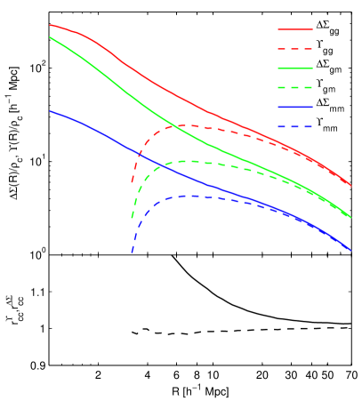
In Fig. 1, we plot both the excess surface mass density and the ADSD $\Upsilon$ defined from the galaxy auto-correlation, matter auto-correlation and their cross-correlation. As galaxies we choose a model for Luminous Red Galaxies (LRGs), as discussed in more detail in §V. We observe that the galaxy-galaxy and galaxy-matter excess surface mass densities are not multiples of the matter correlation function on small scales, so that we expect a cross-correlation different from unity for the bare statistic. This result is seen in the bottom panel of Fig. 1, where the deviations from unity extend to scales above $10\ h^{-1}\text{Mpc}$. Subtracting the signal at $R_{0}=3\ h^{-1}\text{Mpc}$ as in Eq. 12 to get $\Upsilon$, we remove these non-linearities and recover similar shapes for all three functions. As a result, the cross-correlation coefficient is now much closer to unity on all scales above $R_{0}$, as seen in the bottom of Fig. 1.

Figure 2: Left panel: Window functions for $\Upsilon(R;R_{0})$ with $R_{0}=3\ h^{-1}\text{Mpc}$ in real space. We show the window function for $R=5,10,20\ h^{-1}\text{Mpc}$ as green solid, orange dashed and red dash-dotted lines respectively. Right panel: Window functions for $\Upsilon(R;R_{0})$ with $R_{0}=3\ h^{-1}\text{Mpc}$ in $k$-space. We show the products of window function and power spectrum for $R=5,10,20\ h^{-1}\text{Mpc}$ as green solid, orange dashed and red dash-dotted line respectively. For reference we also plot the window for the correlation function as thin lines. Note that we multiplied with $x$ and $k$ respectively to account for the logarithmic scale on the ordinate axis.

Both the projected correlation function and the ADSD are defined by integrals of the correlation function weighted by a kernel. The projected correlation function can be written as

$$w(R)=\int_{0}^{+\infty}\xi(x)W_{w}(x;R)x\,\mathrm{d}\ln{x}\ ,$$ (14)

where the window function is written,

$$W_{w}(x)=\frac{2x}{\sqrt{x^{2}-R^{2}}}\Theta(x-R)\Theta(\sqrt{\chi_{\text{max}}^{2}+R^{2}}-x)\ .$$ (15)

Here $\Theta(x)$ is the Heaviside step function. Thus $w(R)$ has contributions only from scales $x\geq R$, and the window function is peaked at $x=R$.

The ADSD defined in Eq. (12) involves a radial average and subtraction of $w(R)$. Both operations can be included in the integration kernel, and we may write the ADSD as

$$\frac{\Upsilon(R;R_{0})}{\rho_{\text{crit}}}=\int_{0}^{+\infty}\xi(x)W_{\Upsilon}(x;R,R_{0})x\,\mathrm{d}\ln{x}\ .$$ (16)

where the window function for $\Upsilon(R,R_{0})$ is written,

$$W_{\Upsilon}(x;R,R_{0})=\frac{4x}{R^{2}}\left[\sqrt{x^{2}-R_{0}^{2}}\Theta(x-R_{0})-\sqrt{x^{2}-R^{2}}\Theta(x-R)\right]-\frac{2x}{R^{2}}\left[\frac{R^{2}\Theta(x-R)}{\sqrt{x^{2}-R^{2}}}-\frac{R_{0}^{2}\Theta(x-R_{0})}{\sqrt{x^{2}-R_{0}^{2}}}\right]\ .$$ (17)

The scale dependence of the integration kernels reveals the scales in the correlation function that are dominating.

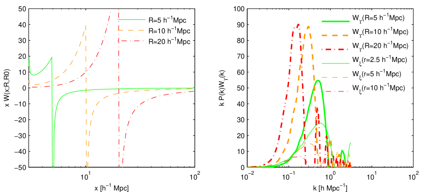
In Fig. 2 we show the window function $W_{\Upsilon}(x;R,R_{0})$ for three different radii and $R_{0}=3\ h^{-1}\text{Mpc}$. Since $\xi(x)$ approximately follows a decreasing power-law, the leading contribution is at the scale $R$, where the sign changes. This sign-change is due to the subtraction $\Delta\Sigma_{\text{AB}}=\rho\left[\overline{w}_{\text{AB}}(R)-w_{\text{AB}}(R)\right]$ and is the same as for $\Delta\Sigma$. For $\Delta\Sigma$ the window is exactly compensated, meaning that it integrates to zero, hence $\Delta\Sigma$ is insensitive to adding a mean density component, the so called mass sheet degeneracy. This compensation is fortunate, since it means that this statistic is insensitive to the long wavelength modes that can move $w(R)$ up and down, i. e. the long wavelength sampling variance affects $w(R)$ on all scales. The compensated window also makes $\Delta\Sigma$ less sensitive to the redshift space distortions, as discussed in §VII. The statistic $\Upsilon$, though not exactly compensated, retains most of these beneficial properties, while at the same time eliminating small scale clustering information.

The scales probed by the statistic $\Upsilon$ are however more obvious in the power spectrum. The conversion from $P(k)\to\Upsilon(R;R_{0})$ can be written as

$$\Upsilon(R;R_{0})=\int P(k)kW_{\Upsilon}(k;R,R_{0})\,\mathrm{d}\ln{k},$$ (18)

where the window function is no longer given by a simple analytical form due to the spherical Bessel functions occurring in the Fourier transform. In Figure 2 we show this window function multiplied with the power spectrum. From this plot we see that for a cutoff radius $R_{0}=3\ h^{-1}\text{Mpc}$, $\Upsilon$ essentially probes scales down to $k\approx 1\ h\ \text{Mpc}^{-1}$. The integrand in (18) is peaked at the scale $k\approx\pi/R$, and is strongly oscillatory on small scales.

For later use we plot the window function for the correlation function $W_{\xi}(k;r)=k^{2}\sin{kr}/{kr}$ that relates $P(k)$ and $\xi(r)$ via $\xi(r)=V/(2\pi)^{3}\int kP(k)W_{\xi}(k;r)\,\mathrm{d}\ln{k}$.

IV Theoretical Modelling of scale dependent bias

Figure 3: Left panel: Non-linear corrections to the real space correlation function as function of radial separation calculated for redshift $z=0.23$. We show the linear (black dotted) and non-linear matter correlation function (thick blue solid) as well as the $B$ (red dash-dotted) and $A$ (green solid and dashed) correction terms. The dashed portion of the graph of $A(r)$ denotes the range where it is negative. Right panel: Perturbation theory fit (dashed) over scales $6\ h^{-1}\text{Mpc}\leq r\leq 80\ h^{-1}\text{Mpc}$ to the measured galaxy-correlation functions (solid) of the luminosity-threshold sample. The fits to $\xi_{\text{gg}}$ (upper green), $\xi_{\text{gm}}$ (central blue) and a joint fit provide consistent results. We are not expecting a good agreement on scales below $r\approx 3\ h^{-1}\text{Mpc}$, where the correlation function is dominated by non-linear clustering.

Figure 4: Left panel: Perturbation terms for the projected surface mass density $w$. We show the non-linear matter correlation function (black dotted) as well as the $w_{\text{B}}$ (red dash-dotted) and $w_{\text{A}}$ (green dashed and solid) terms. Note that the dashed part of the latter curve is negative. Right panel: Perturbation terms for the ADSD and $R_{0}=3\ h^{-1}\text{Mpc}$. Again we show the non-linear matter statistic (black dotted) together with the $\Upsilon_{\text{A}}$ (green dashed and solid) and $\Upsilon_{\text{B}}$ (red dash-dotted) terms. Note that the scale at which the $\Upsilon_{\text{B}}$ term becomes comparable to the non-linear correlation is shifted further out to $R\approx 9\ h^{-1}\text{Mpc}$.

In this section we will use cosmological perturbation theory (for a review see Bernardeau2002 ) to predict the cross-correlation coefficient. Our discussion is based on a Taylor expansion of the galaxy density field in terms of the matter overdensity $\delta$

$$\rho_{\text{g}}=\rho_{0}+\rho_{0}^{\prime}\delta+\frac{1}{2}\rho_{0}^{\prime\prime}\delta^{2}+\frac{1}{6}\rho_{0}^{\prime\prime\prime}\delta^{3}+\epsilon+\mathcal{O}(\delta^{4})$$ (19)

Such an expansion is only valid on scales exceeding the virial radius of dark matter haloes, since it contains no mechanism of halo exclusion or the radial distribution of galaxies within their host halo. Absorbing potentially divergent terms into the bias and shot noise parameters, Smith2007 ; McDonald2006 showed that the auto- and cross-power spectrum of a biased tracer field can be written up to fourth order in the matter density field as

$$P_{\text{gm}}(k) = b_{1}P_{\text{NL}}(k)+b_{2}A(k),$$ (20)

$$P_{\text{gg}}(k) = b_{1}^{2}P_{\text{NL}}(k)+2b_{1}b_{2}A(k)+\frac{b_{2}^{2}}{2}B(k)+N,$$ (21)

where $N$ is the renormalized shot noise, $b_{1}$ and $b_{2}$ are the renormalized bias parameters and $P_{\text{NL}}$ is the non-linear power spectrum. The calculation of the latter can be carried out with any perturbative technique, e. g. standard perturbation theory Bernardeau2002 , renormalized perturbation theory Crocce2006 ; Crocce2006b or Lagrangian perturbation theory. The advantage of this renormalisation of the bias parameters is that there is no artificial smoothing scale involved in the above expansion. However this comes at a price: the bias and shot noise are no longer given ab-initio from theory, but have to be determined empirically.

The correction terms $A(k)$ and $B(k)$ introduced in the above equation are defined as

$$A(k)\!\! = \!\!\int\frac{\mathrm{d}^{3}q}{(2\pi)^{3}}P_{\text{lin}}(q)P_{\text{lin}}(|\bm{k}-\bm{q}|)F_{2}(\bm{q},\bm{k}-\bm{q}),$$ (22)

$$B(k)\!\! = \!\!\int\frac{\mathrm{d}^{3}q}{(2\pi)^{3}}P_{\text{lin}}(|\bm{q}|)\left[P_{\text{lin}}(|\bm{k}-\bm{q}|)-P_{\text{lin}}(q)\right],$$ (23)

where

$$F_{2}(\bm{k}_{1},\bm{k}_{2})=\frac{5}{7}+\frac{1}{2}\frac{\bm{k}_{1}\cdot\bm{k}_{2}}{k_{1}k_{2}}\left(\frac{k_{1}}{k_{2}}+\frac{k_{2}}{k_{1}}\right)+\frac{2}{7}\left(\frac{\bm{k}_{1}\cdot\bm{k}_{2}}{k_{1}k_{2}}\right)^{2}$$ (24)

is the second order standard mode coupling kernel. In the above integrals, one can use the linear power spectrum, because the integrals are already fourth order in the matter density field $\delta$.

Due to the linearity of the expressions in Eqs. (20) and (21) the transformation to real space is straightforward

$$\xi_{\text{gm}}(r)= b_{1}\xi_{\text{NL}}(r)+b_{2}A(r)\ ,$$ (25)

$$\xi_{\text{gg}}(r)= b_{1}^{2}\xi_{\text{NL}}(r)+2b_{1}b_{2}A(r)+\frac{b_{2}^{2}}{2}B(r)\,$$ (26)

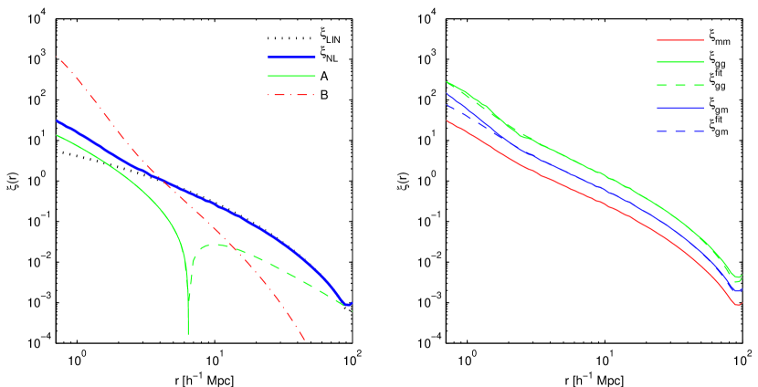
with $\xi_{\text{mm}}(r)=\xi(r)$, and $A(r)$, $B(r)$ being the Fourier transforms of $A(k)$, $B(k)$ respectively. It is easy to show that $B(r)=\xi^{2}-\sigma^{2}\delta^{\text{D}}(\bm{r})$, where $\sigma$ is the variance of the power spectrum. Figure 4 shows the terms contributing to the galaxy auto- and cross-correlation functions as well as a fit to the correlation functions measured in our numerical simulations. The $A(r)$ term is positive on small scales and changes sign at $r\approx 6\ h^{-1}\text{Mpc}$. The $B(r)$ term affecting the auto-correlation dominates over the matter correlation function on scales below $r\lesssim 4\ h^{-1}\text{Mpc}$.

Let us for later convenience define the parameter combination

$$\alpha\equiv\frac{b_{2}}{b_{1}},$$ (27)

As shown by Seljak2009 in the regime where $A(r)\ll\xi(r)$ and $B(r)\ll\xi(r)$ the cross-correlation coefficient can be written as:

$$r_{\text{cc}}^{(\xi)}= \frac{\xi+\alpha A}{\sqrt{\xi(\xi+2\alpha A+\alpha^{2}B/2)}}\ ;$$ (28)

$$\approx 1-\frac{1}{4}\alpha^{2}\frac{B}{\xi}-\alpha^{2}\frac{A^{2}}{\xi^{2}}-\frac{1}{4}\alpha^{3}\frac{AB}{\xi^{2}}\ ;$$ (29)

$$\approx 1-\frac{1}{4}\alpha^{2}\frac{B(r)}{\xi(r)}\ ;$$ (30)

$$\approx 1-\frac{1}{4}\alpha^{2}\xi(r)\ .$$ (31)

Obviously the model predicts a scale dependent cross-correlation that is below unity on small scales and asymptotically approaches unity for increasing $r$. As shown in Seljak2009 , the shape of the cross-correlation coefficient of haloes measured in the simulations is well described by the functional form of the above equation, and the prefactor $\alpha$ is a weak function of halo mass. Clearly this simple theoretical model is not able to cover the non-linear behaviour inside the virial radius after shell-crossing. Qualitatively similar predictions were presented by Matsubara1999 for the peak model of BBKS1986 .

We will now proceed to develop the results repeated here for the readers’ convenience for use in our investigations. A result similar to Eq. (31) remains valid if we consider the projected correlation function, since the integration along the line of sight is a linear operation. We therefore have:

$$w(R)= \int_{-\chi_{\text{max}}}^{+\chi_{\text{max}}}\xi\bigl{(}\sqrt{R^{2}+\chi^{2}}\bigr{)}\mathrm{d}\chi\ ;$$ (32)

$$w_{A}(R)= \int_{-\chi_{\text{max}}}^{+\chi_{\text{max}}}A\bigl{(}\sqrt{R^{2}+\chi^{2}}\bigr{)}\mathrm{d}\chi\ ;$$ (33)

$$w_{B}(R)= \int_{-\chi_{\text{max}}}^{+\chi_{\text{max}}}B\bigl{(}\sqrt{R^{2}+\chi^{2}}\bigr{)}\mathrm{d}\chi\ .$$ (34)

Furthermore, the manipulations that lead to the excess surface mass density, or more generally to the ADSD $\xi(r)\to\Delta\Sigma(R)\to\Upsilon(R)$ are linear in the fields $A$, $B$ and $\xi$. Consequently the corresponding terms have the same order as their underlying statistic and we can write,

$$r_{\text{cc}}^{(\Upsilon)}(R)=1-\frac{1}{4}\alpha^{2}\frac{\Upsilon_{\text{B}}(R)}{\Upsilon_{\text{mm}}(R)}\ .$$ (35)

Note that to evaluate the term $\Upsilon_{\text{B}}(R)$ we only need to replace $\xi(r)$ with $\xi^{2}(r)$ in Eq. (16). The effective value of $\alpha=\left\langle b_{2}\right\rangle/\left\langle b_{1}\right\rangle$ for our galaxy catalogues can be estimated using the mean bias parameters from the peak-background-split Sheth1999 ; Scoccimarro2001 ,

$$\left\langle b_{i}\right\rangle=\frac{\int n(M)\left\langle N(M)\right\rangle b_{i}(M)dM}{\int n(M)\left\langle N(M)\right\rangle\mathrm{d}M}\ \ i=1,2,$$ (36)

where $n(M)$ is the halo mass-function and $\left\langle N(M)\right\rangle$ is the halo occupation number. For the rest of this work we will adopt $\alpha=0.26$, which is close to peak-background split predictions Seljak2009 . An alternative approach, accounting for the renormalised nature of the parameters, would be to fit for the model parameters by matching theoretical and measured correlation functions as shown in the right panel of Figure 4. This second approach provides results that are consistent with the peak-background-split result.

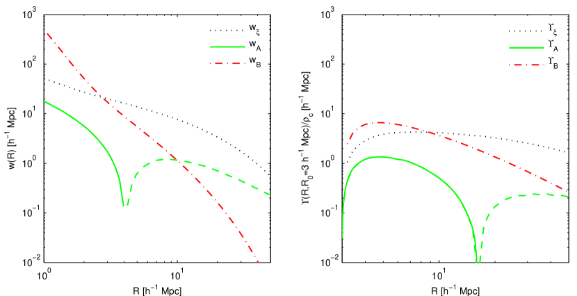
In Figure 4 we plot the correction terms contributing to the projected correlation function and the ADSD. The prerequisite for the Taylor expansion to be applicable is that the correction terms $w_{\text{A}}/w_{\text{mm}}\ll 1$ and $w_{\text{B}}/w_{\text{mm}}\ll 1$ or $\Upsilon_{\text{A}}/\Upsilon_{\text{mm}}\ll 1$ and $\Upsilon_{\text{B}}/\Upsilon_{\text{mm}}\ll 1$. We see that these assumptions are violated below $R=3\ h^{-1}\text{Mpc}$ for the projected correlation function and below $R=9\ h^{-1}\text{Mpc}$ for the ADSD. For the non-linear correlation function $\xi$ we use the matter correlation function measured in the simulations.

V Numerical Modelling

With modern large supercomputers and well developed algorithms it is now possible to model the evolution of the dark matter density field on cosmological scales reasonably well. However, what one observes are not dark matter haloes but galaxies. Supplementing the distribution of dark matter in a simulation box with the galaxy distribution corresponding to a particular galaxy sample would in principle require an understanding of the process of galaxy formation. An ab initio treatment of all the baryonic processes is difficult, and requires, e. g. full treatment of the hydrodynamics, atomic and radiative heating and cooling of gas at high resolution. Owing to the large computational cost, state of the art simulations are restricted to relatively small scales and lack sufficient volume to extract statistically relevant information on cosmological scales Agertzetal2009 . Thus we pursue a statistical approach to populate the haloes identified in a suite of large-scale $N$-body simulations with galaxies.

V.1 The Simulations

Our numerical results are based on the Zürich horizon “zHORIZON” simulations, a suite of $30$ pure dissipationless dark matter simulations of the $\Lambda$CDM cosmology in which the matter density field is sampled by $N_{p}=750^{3}$ dark matter particles. The box length of $1500\ h^{-1}\text{Mpc}$, together with the cosmological parameters given in Table 1, then implies a particle mass of $M_{\text{dm}}=5.55\times 10^{11}\ h^{-1}M_{\odot}$. This simulation volume enables high precision studies of the fluctuations in the $\Lambda$CDM model on scales up to a few hundred comoving megaparsecs Smith2008a .

The simulations were carried out on the ZBOX2 and ZBOX3 computer-clusters of the Institute for Theoretical Physics at the University of Zurich using the publicly available GADGET-II code Springel2005 . The force softening length of the simulations used for this work was set to $60\ h^{-1}\text{kpc}$, consequently limiting our considerations to larger scales. The transfer function at redshift $z=0$ was calculated using the CMBFAST code of Seljak1996 and then rescaled to the initial redshift $z_{i}=50$ using the linear growth factor. For each simulation, a realisation of the power spectrum and the corresponding gravitational potential were calculated. Particles were then placed on a Cartesian grid of spacing $\Delta x=2\ h^{-1}\text{Mpc}$ and displaced according to a second order Lagrangian perturbation theory. The displacements and initial conditions were computed with the 2LPT code of Scoccimarro1998 ; Crocceetal2006 .

The cosmological parameters for the simulations were inspired by the best fit values released by the WMAP3 analysis of the cosmic microwave background Spergel2003 ; Spergel2007 , and can be taken from Table 1. Throughout the paper we adopt this parameter set as our fiducial cosmological model.

Our effective volume is $V=27\ h^{-3}\text{Gpc}^{3}$. For each of the simulation outputs, gravitationally bound structures were identified using the B-FoF algorithm kindly provided by Volker Springel. The linking length in this Friends-of-Friends halo finder was set to $0.2$ of the mean inter-particle spacings, and haloes with less than $20$ particles were rejected. All together we resolve haloes with $M>1.2\times 10^{13}\ h^{-1}M_{\odot}$.

	$\Omega_{\text{m}}$	$\Omega_{\Lambda}$	$h$	$\sigma_{8}$	$n_{s}$	$w$	$N_{\text{e}}$
FID	$0.25$	$0.75$	$0.7$	$0.8$	$1.0$	$-1$	8
C1	$0.25$	$0.75$	$0.7$	$0.8$	$0.95$	$-1$	4
C2	$0.25$	$0.75$	$0.7$	$0.9$	$1.0$	$-1$	4
C3	$0.2$	$0.8$	$0.7$	$0.8$	$1.0$	$-1$	4
C4	$0.3$	$0.7$	$0.7$	$0.8$	$1.0$	$-1$	4

Table 1: Cosmological parameters adopted for our investigations. Matter density parameter, dark energy density parameter, dimensionless Hubble parameter $H_{0}=100h\ \text{km}\ \text{s}^{-1}\ \text{Mpc}^{-1}$, power spectrum normalisation, primordial power spectrum slope, dark energy equation of state $p=\omega\rho$, number of simulation outputs. The first line is our fiducial model. In order to evaluate the cosmology dependence of our results we use four other cosmologies denoted as C1-C4.

V.2 HOD Modelling I - Luminosity Threshold Sample

The statistical model used to populate the haloes with galaxies is known as the Halo Occupation Distribution (HOD), which is closely related to the Halo Model of Large Scale Structure (for a review see Cooray2002 ). The HOD assumes that galaxies form in the dark matter potential wells, because only there can baryons cool with sufficient efficiency. To translate this idea into a quantitative model, one must fix the following ingredients:

1. Number of galaxies that occupy a halo of mass $M$

2. Radial distribution of galaxies within the halo

Theories of galaxy formation suggest a division into central and satellite galaxies. Central galaxies are those that reside at the minimum of the potential well for host dark matter haloes. In contrast, satellite galaxies orbit the central galaxy and are presumed to have their own associated subhalo within the larger host halo. Furthermore we will assume that the number of satellite galaxies is a function of host halo mass only and neglect any environmental influences. The basic assumption of the model is that bright galaxies will not be able to live in low mass haloes, since there is not enough cold gas to form such galaxies. Equivalently, the halo mass can be represented by the virial radius $r_{\text{vir}}$, defined by the condition that the density within $r_{\text{vir}}$ equals 200 times the critical density $\rho_{\text{crit}}$.

Let us start by considering the HOD required to model a luminosity-threshold sample of galaxies, and later in §V.3 we will describe the necessary adaptations required for the more complex luminosity bin sample.

First, we decide whether a halo of given mass contains a central galaxy at its potential minimum. It is reasonable to assume that a threshold in galaxy luminosity corresponds to a threshold in halo mass, but in practice it is necessary to take into account the scatter in the luminosity-mass relationship. We do this by appropriately smoothing the mass threshold. Following Reid2008 ; Padmanabhan2008 , we take the mean number of central galaxies occupying a mass $M$ halo to be:

$$\left\langle N_{\text{cen}}\right\rangle=\text{erfc}\left[-\frac{\ln\left(M/M_{\text{cut}}\right)}{\sqrt{2}\sigma}\right],$$ (37)

where $\text{erfc}(x)=1-\text{erf}(x)$ is the complementary error function, and $M_{\rm cut}$ and $\sigma$ are parameters to be determined from the data. This relationship is then used as a sampling probability for the Bernoulli distribution: operationally this amounts to drawing a random number, $T\in[0,1]$, and if $T<\left<N_{\rm cen}\right>$ then we place a central. This central galaxy is assumed to be formed by the baryons cooling in the dark matter potential well and subsequent collisions with satellite galaxies that approach the halo centre due to dynamical friction.

Satellite galaxies that orbit the halo center mostly originate from the merging of haloes already containing a central galaxy. Subhalo counts in high resolution $N$-body dark matter simulations have shown that the number of satellite galaxies follows a Poisson distribution around an asymptotic power law Kravtsov2004 . Hence we take,

$$\left\langle N_{\text{sat}}\right\rangle_{\text{c}}(M)=\begin{cases}\left(\frac{M-M_{\text{min}}}{M_{1}}\right)^{\alpha},&\text{if }M>M_{\text{min}}\wedge N_{\text{cen}}\neq 0\\ 0,&\text{otherwise}\ ,\end{cases}$$ (38)

which introduces another three parameters to be determined: $M_{\rm min}$, $M_{1}$ and $\alpha$. Finally, as a further constraint we impose the condition that satellite galaxies can only reside in haloes already containing a central galaxy.

The satellite galaxies are expected to be situated in the subhaloes orbiting the halo centre. Our simulations lack sufficient resolution to identify such dark matter substructures, so we instead sample the galaxy positions from the dark matter particle positions. Compared to a galaxy distribution following a profile this approach has several advantages. Firstly, we avoid the assumption of a functional form for the halo profile, instead profiting from the full triaxial dark matter distribution. Secondly, we can assign the dark matter particle velocities to the galaxies, which is useful for studies of the redshift space distortions.

All together, we have five-dimensional parameter space spanned by $\{M_{\text{cut}},\sigma,M_{\text{min}},M_{1},\alpha\}$. We vary these five parameters in order to generate galaxy catalogues that can reproduce observed galaxy clustering and galaxy-galaxy lensing measurements for the two LRG samples described in Mandelbaum2005 and §V.4 below. For each point in parameter space, we generate four galaxy catalogues per simulation using different random seeds. We then calculate the average of the clustering statistics of these four catalogues to remove some of the stochasticity intrinsic to the HOD model, and finally compare to the data. To reduce the dimension of the parameter space and thus the computational costs, we use the observed abundance of the LRG sample to impose a further constraint on the cutoff mass $M_{\text{cut}}$ by demanding

$$\overline{n}_{\text{obs}}=\int\mathrm{d}Mn(M)\left\langle N_{\text{tot}}\right\rangle,$$ (39)

where $n(M)$ is the halo mass-function and the mean total number of galaxies per halo is given by

$$\left\langle N_{\text{tot}}\right\rangle=\left\langle N_{\text{cen}}\right\rangle\bigl{[}\left\langle N_{\text{sat}}\right\rangle+1\bigr{]},$$ (40)

where the form of $\left\langle N_{\text{cen}}\right\rangle$ accounts for the scatter in the luminosity-mass relationship. Finally, we end up with a 4-dimensional parameter space, which is sampled on a grid of points, for each of which we calculate $M_{\text{cut}}$.

Figure 5: Mean galaxy number per halo as a function of halo mass for the luminosity-threshold sample and our best fit parameters from Table 2. We show the number of central galaxies (blue dash-dotted), satellite galaxies (red dashed) and the total number of galaxies (black solid). Note that the satellite number exceeds unity only for haloes with $M>6\times 10^{14}\ h^{-1}M_{\odot}$, corresponding to virial radii exceeding $r_{\text{vir}}\gtrsim 2\ h^{-1}\text{Mpc}$.

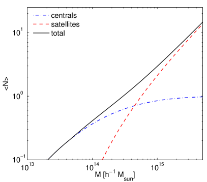
Figure (5) shows the mass dependence of the central, satellite and total halo occupation number for our best fit luminosity-threshold galaxy samples. The total occupation number is dominated by the central galaxies residing in the highly abundant low-mass haloes. Satellite galaxies start to dominate only for masses of $M\approx 4\times 10^{14}\ h^{-1}M_{\odot}$.

V.3 HOD Modelling II - Luminosity Bin Sample

To model a luminosity binned galaxy sample it is necessary to apply some minor changes to our HOD modelling. Firstly, the halo mass of the central galaxies will be a window rather than a threshold. Secondly, we must drop the constraint that satellite galaxies live only in haloes already hosting a central galaxy, because faint galaxies may orbit in heavier haloes (that already host a central above the luminosity cutoff) as satellites. For simplicity, we do not use the information about central LRGs from the bright sample, but rather model the two samples independently. Again the number of central galaxies is assumed to follow a Bernoulli distribution, but with mean given by

$$\left\langle N_{\text{cen}}\right\rangle=\frac{1}{4}\text{erfc}\left[-\frac{\ln{M/M_{\text{cut},1}}}{\sqrt{2}\sigma}\right]\text{erfc}\left[\frac{\ln{M/M_{\text{cut},2}}}{\sqrt{2}\sigma}\right]\ ,$$ (41)

where we have assumed that the central galaxy distribution is symmetric in $\log M$ and that the mass-luminosity scatter is independent of mass. This parametrisation introduces three free parameters: $[M_{\text{cut,1}},M_{\text{cut,2}}]$ with a smoothing parameter $\sigma$. One may of course conceive more complicated window functions, however this approach introduces the least number of additional free parameters into the modelling procedure whilst being flexible enough to describe the data.

For the satellite galaxy distribution, we again assume that the number follows a Poisson distribution, with mean specified by

$$\left\langle N_{\text{sat}}\right\rangle_{\text{c}}(M)=\begin{cases}\left(\frac{M-M_{\text{min}}}{M_{1}}\right)^{\alpha},&\text{if }M>M_{\text{min}}\\ 0,&\text{otherwise}\ .\end{cases}$$ (42)

Thus in total we must constrain six free parameters. However, we may reduce the dimensionality of the problem by calculating the appropriate lower mass cutoff $M_{\text{cut,1}}$ for each of the points in the five-dimensional space spanned by $\{M_{\text{cut,2}},\sigma,M_{1},M_{\text{min}},\alpha\}$ according to Eq. (39).

V.4 Reference Sample

In this study, we develop our analysis for application to the SDSS spectroscopic LRG sample York2000 ; Eisenstein2001 . The LRGs are typically bright red ellipticals that are volume-limited within a much larger volume than the main galaxy sample of the SDSS. Thus they are frequently used as an efficient tracer of large scale structure. Furthermore, since the LRGs have been shown to live in the most massive haloes of the Universe Mandelbaum2006 ; Reid2008 ; Reid2008a ; Zheng2008 , they can be effectively probed with our $N$-body simulations.

The specific LRG samples that we tune our HODs to are presented in Mandelbaum2006 . We model the galaxy-galaxy lensing from that study, along with new projected correlation function measurements of the same samples. In Mandelbaum2006 , the LRG samples were split into two sub-samples, LRGbright and LRGfaint, based on the $r$-band luminosities $k+e$-corrected to $z=0$. LRGbright is a luminosity-threshold sample with a number density of $\overline{n}=4\times 10^{-5}h^{3}\ \text{Mpc}^{-3}$, whereas LRGfaint is a luminosity-bin sample with a number density of $\overline{n}=8\times 10^{-5}h^{3}\ \text{Mpc}^{-3}$. As a result, different strategies must be applied when modelling the sub-samples, as discussed in the previous two subsections. The LRG sample under consideration spans a redshift range $0.15\leq z\leq 0.35$ with an effective redshift of $z_{\text{eff}}=0.24$. This effective redshift was derived from the lensing analysis, since higher redshift lens galaxies are downweighted by the lower number of source galaxies behind them. As shown in Tegmark2006 ; Padmanabhan2008 , the clustering amplitude of LRGs is independent of redshift due to a subtle balance between the redshift evolutions of bias and growth. Therefore we use the simulation outputs at $z_{\text{sim}}=0.23$, very close to the effective lensing redshift, for our numerical analysis.

V.5 Fit results

In Table 2, we quote the inferred HOD parameters for the bright and faint samples when using the fiducial cosmological model. We decided to use the full covariance matrix for the fitting since there are non-negligible correlations between $R$-bins, both in the lensing and clustering measurements. The noise in the covariance matrix increases the inferred $\chi^{2}$, an effect that has previously been investigated by Hirata2004 and we think that theoretical covariance predictions could improve the analysis. Imperfect modelling might of course also arise from the fact that our simulation cosmology is not a perfect representation of the real Universe. Due to the computational costs per model and the high dimensionality of the parameter space we have to restrict to coarse sampling of parameter space. It is however not our goal to precisely constrain the HOD parameters, but rather to obtain reasonable galaxy catalogues for the two LRG samples under consideration and use them to test the $\Upsilon$ statistics. We compare to the HOD parameters obtained by Reid2008 , who used an equivalent model, finding a reasonable agreement, once we account for the fact that they model the full LRG sample.

The galaxy catalogues have relatively low satellite fractions of $\sim 4.5\%$ for the threshold sample and $\sim 10\%$ for the bin sample. Fitting for the bias on linear scales ($18\ h^{-1}\text{Mpc}\leq r\leq 90\ h^{-1}\text{Mpc}$) we obtain $b=2.20\pm 0.03$ and $b=1.97\pm 0.03$ for the threshold and bin sample, respectively.

	$\overline{n}$	$M_{1}$	$M_{\text{cut,l}}$	$M_{\text{cut,u}}$	$\alpha$	$\sigma$	$M_{\text{min}}$
LRGbright	$4.0$	$40.0$	$17.8$	—	$1.05$	$1.68$	$4.6$
LRGfaint	$8.0$	$45.0$	$5.0$	$12.4$	$0.40$	$1.55$	$5.7$

Table 2: Best fit HOD parameters for the faint (f) and bright (b) sample: comoving number density, power law normalisation, low mass cutoff, high mass cutoff, power law exponent, smoothing and lower satellite cutoff. The number densities are in units of $1\times 10^{-5}\ h^{3}\ \text{Mpc}^{-3}$, and masses are in units of $10^{13}\ h^{-1}M_{\odot}$.

Figure 6: Cross-correlation coefficient of the ADSD $\Upsilon$ for the luminosity-threshold (left panel) and luminosity bin sample (right panel). The trivial case $R_{0}=0$ (black with errorbars), corresponding to bare $\Delta\Sigma$, leads to a cross-correlation coefficient that is far from unity and furthermore strongly scale dependent. If we instead choose $R_{0}=3\ h^{-1}\text{Mpc}$ (blue with errorbars), inspired by the virial radii of the haloes under consideration, we restore a cross-correlation coefficient close to unity on the $4\%$ level for all scales $R>R_{0}$. Furthermore, we can model the residual scale dependence reasonably well using the perturbation theory expression of Eq. (35) (solid blue line), whereas the the bare $\Delta\Sigma$ deviates from the corresponding perturbation theory result (black dash-dotted). Since the Taylor expansion is no longer justified for scales below $R=8\ h^{-1}\text{Mpc}$, we also plot the full expression according to Equation (43) (red dashed) for $\Upsilon$.

Figure 7: Reconstructed matter ADSD for the luminosity-threshold (left panel) and luminosity-bin sample (right panel). We plot the inferred value from the simulations including corrections for $r_{\text{cc}}\neq 1$ as well as the non-linear prediction derived from the measured matter-correlation of the simulations (red solid line) and the linear theory value (black dashed line). The non-linear correlation is well reproduced by the reconstruction, whereas there are remarkable deviations from linear theory on small scales.

VI Numerical Results

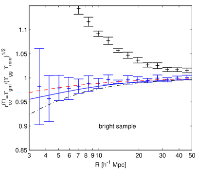
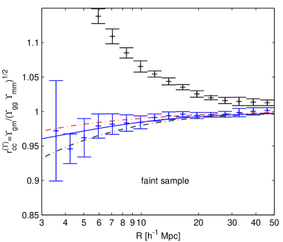
To replicate the cross-correlation coefficient between galaxies and matter that would be expected from real observational data, we use the artificial galaxy catalogues described in the previous section to measure all of the statistics of interest. Figure 7 shows the resulting cross-correlation coefficients of the luminosity-threshold (left panel) and luminosity-bin (right panel) galaxy catalogues and two values of $R_{0}$. The ADSD is measured by counting the number of pairs in cylinders with length $2\chi_{\text{max}}=100\ h^{-1}\text{Mpc}$ in real space. The errorbars shown in these figures are derived from the standard-deviation between the eight simulation volumes and thus represent the cosmic variance. We again see that $\Delta\Sigma$ (black), corresponding to $R_{0}=0$, leads to a cross-correlation coefficient that is strongly scale dependent and different from unity, with 5–10% deviations at $10\ h^{-1}\text{Mpc}$. However, if we choose $R_{0}=3\ h^{-1}\text{Mpc}$, then we find that a cross-correlation coefficient close to unity (blue with errorbars), with $r_{\text{cc}}=0.96$ at $4\ h^{-1}\text{Mpc}$, as predicted by perturbation theory for biased tracers Seljak2009 . Furthermore, we observe this behaviour for both the luminosity-bin sample and the luminosity-threshold sample. This consistency suggests that the cross-correlation coefficient is largely independent of the specific choice of the HOD used to generate the galaxy catalogues, which is again consistent with the arguments in Seljak2009 that the cross-correlation coefficient is nearly universal in the sense of being only weakly dependent on the halo mass. The theoretical prediction of Eq. (35) is plotted in Figure 7 as the blue solid line. For the latter we use $\xi_{\text{NL}}$ to predict $\Upsilon_{\text{mm}}=\Upsilon_{\xi}$ and $\Upsilon_{\text{B}}=\Upsilon_{\xi^{2}}$. We furthermore compare to the full, non-expanded expression

$$r_{\text{cc}}^{(\Upsilon)}(R)=\frac{\Upsilon_{\xi}+\alpha\Upsilon_{\text{A}}}{\sqrt{\Upsilon_{\xi}(\Upsilon_{\xi}+2\alpha\Upsilon_{\text{A}}+\alpha^{2}\Upsilon_{\text{B}}/2})},$$ (43)

shown as the red-dash dotted line, whose range of validity is bounded by the breakdown of perturbation theory rather than the relative magnitude of the perturbation terms. Given the statistical uncertainties of the direct simulation measurements, both expressions are viable because the difference is $\sim 2\%$ on the smallest scales considered.

The results discussed above suggest, that we may invert Eq. (13) through the following,

$$\Upsilon_{\text{mm}}(R)=\frac{\Upsilon_{\text{gm}}^{2}(R)}{\Upsilon_{\text{gg}}(R)r_{\text{cc}}^{2}}\propto\Omega_{\text{m}}^{2}\sigma_{8}^{2}\ .$$ (44)

The resulting statistic depends on the matter correlation function and squared matter density, which is the usual parameter dependence of weak lensing measurements. This dependence enables us to constrain cosmological parameters. Our theoretical model provides us with the scale dependent correction factor $r_{\text{cc}}^{(\Upsilon)}$. Note that the cross-correlation coefficient is very close to unity on all scales shown and even using $r_{\text{cc}}=1$ is acceptable given current observational constraints. However, future observations will measure galaxy-galaxy lensing with much higher statistical precision. The extraction of the full amount of information contained in these measurements will require an accurate modelling of $r_{\text{cc}}$. As argued in Seljak2009 this can be done in a relatively robust and model independent way.

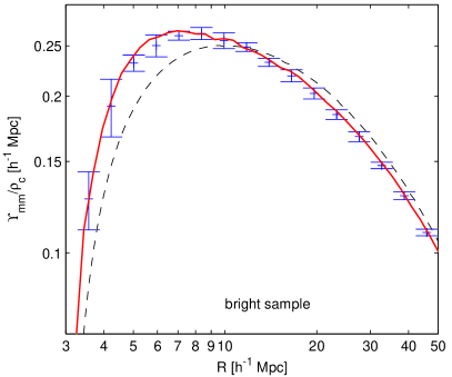
In Figure 7, we show the results of such a reconstruction based on eight galaxy catalogues with the corresponding cosmic variance errors. This reconstruction includes the correction for the deviations of the cross-correlation coefficient from unity. We see that the non-linear $\Upsilon_{\text{mm}}^{\text{(nl)}}$ is reproduced with high accuracy, whereas the linear theory prediction $\Upsilon_{\text{mm}}^{\text{(lin)}}$ deviates from our simulation result. This finding is expected, because in Eq. (12) we subtract $\Delta\Sigma(R_{0})$ at $R_{0}=3\ h^{-1}\text{Mpc}$, which is already at a non-linear scale. As we go to larger scales this contribution is suppressed by $R_{0}^{2}/R^{2}$ and we slowly approach the linear theory predictions.

Our numerical study implicitly uses the distant observer approximation, since we project the density field in the simulation along one of the three Cartesian coordinate axes. In a real observation, the lines of sight to two nearby galaxies or to a foreground lens and a background source galaxy are inclined. The question of whether the two statistics agree is related to the extent to which the angular and the 2D projected power spectra agree. As discussed in LoVerde2008 , the angular power spectrum corresponds to the 2D power spectrum if the Limber approximation Limber1953 is valid. The LRG sample under consideration in our study has a median redshift of $z=0.23$ corresponding to a comoving distance $\chi_{\text{l}}=650\ h^{-1}\text{Mpc}$. Together with the maximum projection length $\chi_{\text{max}}=\pm 100\ h^{-1}\text{Mpc}$ and the maximum transverse distance to the galaxy $R_{\text{max}}=70\ h^{-1}\text{Mpc}$, this corresponds to a maximum angle of $\theta_{\text{max}}=7.3^{\circ}$. The Limber approximation is typically precise to $<1\%$ for $l\approx\pi/\theta>10$ Smith2009b , corresponding to $\theta<18^{\circ}$, and thus we can safely use the Cartesian analysis as an approximation for the observations.

VII Sources of Errors

Accurate studies of cosmological parameters require a careful consideration of all effects that might change the signal. In this section, we explore how large-scale redshift space distortions and the difference between lensing and galaxy clustering window functions impacts the reconstruction of the matter clustering. Finally, we will discuss how strongly the radial bins are correlated.

VII.1 Influence of Redshift Space Distortions

Figure 8: Left panel: Residual effect of redshift space distortions on the projected galaxy-galaxy auto-correlation function $w_{\text{gg}}$. We show the simulation measurements for the bright sample as crosses with errorbars for $\chi_{\text{max}}=50\ h^{-1}\text{Mpc}$ (upper blue) and $\chi_{\text{max}}=100\ h^{-1}\text{Mpc}$ (lower red) and the corresponding linear theory predictions. Right panel: Residual effect on the annular differential surface density $\Upsilon_{\text{gg}}(R;R_{0}=3\ h^{-1}\text{Mpc})$ for the same integration lengths. As on the left panel, the upper blue curve and points correspond to $\chi_{\text{max}}=50\ h^{-1}\text{Mpc}$ whereas the lower red curve and points correspond to $\chi_{\text{max}}=100\ h^{-1}\text{Mpc}$.

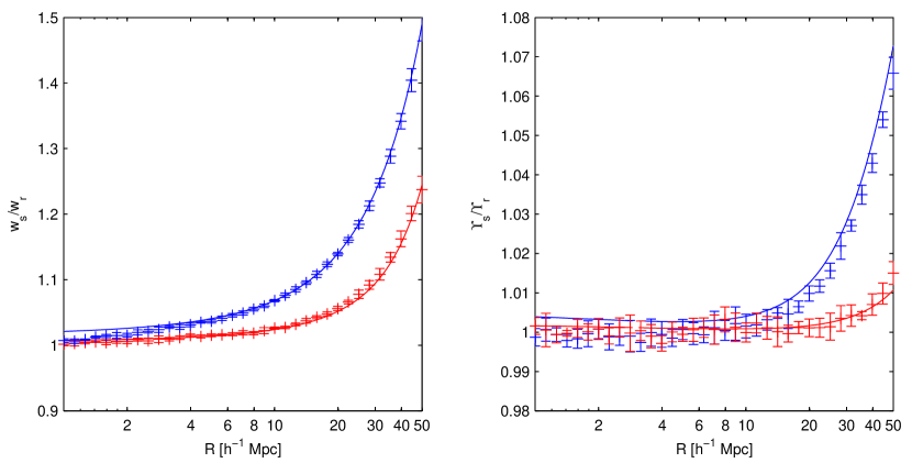
In large redshift surveys, such as the SDSS York2000 or 2dF Colless2001 , the radial distance to a galaxy is inferred from the recession velocity, under the assumption of a perfect Hubble law. In reality, the coherent motions of galaxies and their virial motions inside haloes will add to the redshift and thus distort the inferred distance. In the linear regime, on large scales these redshift space distortions can be quantified using linear theory, neglecting virial motions within the bound structures (for a review see Hamilton1998 ). Following Kaiser1987 we can write the galaxy power spectrum in redshift space in the plane parallel projection as

$$P_{\text{s}}(k)=P_{\text{r}}(k)\left[1+\beta\mu^{2}\right]^{2}\ ,$$ (45)

where $P_{\text{r}}(k)$ is the real space power spectrum of the tracer, $\mu=\bm{k}\cdot\hat{\bm{x}}/k$ is the position angle with respect to the redshift axis $\hat{\bm{x}}$ and $\beta=f(a)/b_{1}(a)$, where $f(a)\equiv\mathrm{d}\ln D/\mathrm{d}\ln a$ is the logarithmic growth rate of fluctuations. We obtain this directly by numerically evaluating the exact expression:

$$f(a)=\frac{\mathrm{d}\ln{H(a)}}{\mathrm{d}\ln{a}}+\frac{a}{(aH(a))^{3}}\frac{1}{\int_{0}^{a}\mathrm{d}a^{\prime}(a^{\prime}H(a^{\prime}))^{-3}}\ .$$ (46)

In what follows it will be convenient to rewrite Eq. (45) in terms of the Legendre polynomials $L_{l}(\mu)$

$$P_{\text{s}}(k)=P_{\text{r}}(k)\left[\alpha_{0}L_{0}(\mu)+\alpha_{2}L_{2}(\mu)+\alpha_{4}L_{4}(\mu)\right]\ ,$$ (47)

where the coefficients are given by:

$$\alpha_{0}(\beta)= 1+\frac{2}{3}\beta+\frac{1}{5}\beta^{2}\ ;$$ (48)

$$\alpha_{2}(\beta)= \frac{4}{3}\beta+\frac{4}{7}\beta^{2}\ ;$$ (49)

$$\alpha_{4}(\beta)= \frac{8}{35}\beta^{2}\ .$$ (50)

The redshift space correlation function is then obtained by a Fourier transform of the power spectrum:

$$\xi_{\rm gg,s}(r,\nu) = \frac{V}{(2\pi)^{3}}\int_{0}^{\infty}\mathrm{d}kk^{2}P_{\text{r}}(k)\int_{-1}^{1}\mathrm{d}\mu\left[1+\beta\mu^{2}\right]^{2}$$ (51)

$$\times\int_{0}^{2\pi}\mathrm{d}\varphi\exp{\left[i\bm{k}\cdot\bm{x}\right]}\ ;$$

$$= \sum_{l=0}^{2}\alpha_{2l}(\beta)\xi_{2l}(r)L_{2l}(\nu),$$ (52)

where $\nu$ is the angle between $\bm{r}$ and the axis along which the redshift space distortion is present, i.e. $\nu=\hat{\bm{x}}\cdot\hat{\bm{r}}=x/r$. The correlation function multipoles in the above equation are defined as

$$\xi_{2l}(r)=(-1)^{l}\frac{V}{2\pi^{2}}\int_{0}^{\infty}\mathrm{d}kk^{2}P_{\text{r}}(k)j_{2l}(kr)\ ,$$ (53)

where the $j_{l}$ are the spherical Bessel functions: $j_{l}(x)=J_{l+1/2}(x)/\sqrt{2x}$. We note that the above formulae are equivalent to the formulation of Hamilton1992 .

For our investigations, we are mainly concerned with the projected correlation function or the closely related excess surface mass density. The common assumption is that the integration along the line of sight removes redshift space distortions. This assumption, however, would only be correct in the limit of an infinite radial projection window, which is not used in practice. Integrating Eq. (52) along the line of sight, we obtain

$$w_{\text{gg,s}}(R) = \int_{-\chi_{\text{max}}}^{\chi_{\text{max}}}\xi_{\rm gg,s}(r,\nu)\mathrm{d}\chi$$ (54)

$$= 2\sum_{l=0}^{2}\alpha_{2l}(\beta)\int_{0}^{\chi_{\text{max}}}\!\!d\chi\,\xi_{2l}\left(\sqrt{\chi^{2}+R^{2}}\right)$$

$$\times\ L_{2l}\left(\frac{\chi}{\sqrt{\chi^{2}+R^{2}}}\right)\ .$$

We shall use the above result to calculate the linear theory predictions for the projected correlation functions in redshift space.

Figure 9: Correction factors that must be applied to the galaxy clustering measurements in order to remove redshift space distortions and to construct a quantity equivalent to the lensing signal. The total correction (red solid) is a product of a window correction (blue dashed) and a redshift correction (green dash-dotted). Left panel: Projected galaxy-galaxy auto-correlation function $w_{\text{gg}}$. The size of the corrections is quite remarkable on the largest scales. The apparent effects on scales below $10\ h^{-1}\text{Mpc}$ arise from the flattening of the linear power spectrum on these scales. Furthermore the correlation on these scales would be affected by the finger-of-god effects not included in our analysis. Right panel: Annular differential surface density for $R_{0}=3\ h^{-1}\text{Mpc}$. The residual correction is much smaller, $3\%$ on the typical scales probed by galaxy-galaxy lensing.

In Figure 8, we plot the ratio of the real to redshift space projected correlation functions for the bright LRG galaxy sample with $b=2.2$. We clearly see that the commonly used integration length of $\chi_{\text{max}}=50\ h^{-1}\text{Mpc}$ leads to residual distortions of about $40\%$ on scales $R\approx 50\ h^{-1}\text{Mpc}$. These residual redshift space effects on the projected correlation function were previously discussed by Tinker2006 ; Tinker2007 (see also Padmanabhan2007 ). Moreover, we see that on these scales the linear theory prediction is a very good description to the effects that we observe in our simulations. The difference between linear theory and simulation, on small scales, arises from the fact that we do not model the virial motions, which cause the fingers-of-god. Furthermore, the non-linear correlation function is more cuspy than the linear correlation function on small scales. Therefore the linear predictions in redshift space are boosted in amplitude by the compression along the line of sight. The non-linear projected correlation function is however much more influenced by the increased small-scale clustering, and thus at small separations transverse to the line of sight, it is less sensitive to the compression.

Even though the linear prediction is a good description of the effect, removing it requires knowledge of the redshift space distortion parameter $\beta$, which requires knowledge of both the cosmological model and bias. Since these are not known a priory but instead they must be determined from the data. To do this accurately an iterative approach is needed, which complicates the analysis and ultimately limits the precision. Thus, it is advantageous if these corrections can be made as small as possible from the onset. As we show in the right panel of Fig. 8, for the ADSD statistic $\Upsilon$ much smaller residual corrections are required. The reduction is dramatic, with an order of magnitude smaller effect at the same scale and for the same radial window. As discussed above, this reduction results from the compensated nature of these statistics, which makes them much less sensitive to the long wavelength fluctuations, so that the limit $\chi_{\text{max}}\rightarrow\infty$ is approached faster. This makes these statistics more attractive for practical applications than the projected correlation function $w$. In the context of galaxy clustering, similar compensated statistics have been proposed in Padmanabhan2007 . Note that for lensing the typical radial window is hundreds of $\ h^{-1}\text{Mpc}$ wide, and for $\Delta\Sigma_{\text{gm}}$ or $\Upsilon_{\text{gm}}$ the effects of redshift space distortions can be completely neglected on scales below $R\approx 100\ h^{-1}\text{Mpc}$.

The analytical predictions for the impact of redshift space distortions on $\Upsilon$ and $w$ are based on the Kaiser model and thus make use of the flat sky and distant observer approximation. However, as we showed above, the ADSD is very robust to redshift space distortions with residual corrections on the $\mathcal{O}(1\%)$ level. Due to the smallness of the correction and since our study is restricted to transverse separations that are small compared to the line of sight distance to the galaxies, our treatment is justified.

VII.2 Dependence on projection length

Figure 10: Columns extracted from the correlation matrix of the bright LRG sample Left panel: $\text{Corr}(w)$ Central panel: $\text{Corr}(\Delta\Sigma)$ Right panel: $\text{Corr}(\Upsilon)$, where the vertical dashed line shows the cutoff radius $R_{0}$. Comparing the correlation matrices for $w$ and $\Delta\Sigma$ it is clear that the width of the off-diagonal contributions is larger for the projected correlation function than for the excess surface mass density. The same remains true if one compares the correlation of the ADSD and the projected correlation function.

Our final goal is to compare a galaxy-matter cross-correlation corresponding to a very broad lensing window and a galaxy-galaxy auto-correlation that is calculated from a narrow top-hat window and thus, in contrast to the lensing, subject to redshift space distortions. In this context it is necessary to devise a correction that accounts for both the redshift space distortions and the different window functions. We already discussed the redshift space effects and saw that they can be described by a scale dependent factor $\Upsilon_{\text{gg,r}}^{\text{(clust)}}/\Upsilon_{\text{gg,s}}^{\text{(clust)}}$ given by linear theory. Here we use the superscript “clust” to denote that this statistic is measured with the top-hat window. A similar numerical factor can be used to transfer from the clustering to the lensing window $\Upsilon_{\text{gg,r}}^{\text{(lens)}}/\Upsilon_{\text{gg,r}}^{\text{(clust)}}$. The corrected galaxy correlation function corresponding to the lensing measurements then reads as:

$$\Upsilon_{\text{gg,r}}^{\text{(lens)}} = \Upsilon_{\text{gg,s}}^{\text{(clust)}}\frac{\Upsilon_{\text{gg,s}}^{\text{(lens)}}}{\Upsilon_{\text{gg,s}}^{\text{(clust)}}}\ ;$$ (55)

$$= \Upsilon_{\text{gg,s}}^{\text{(clust)}}\underbrace{\frac{\Upsilon_{\text{gg,r}}^{\text{(clust)}}}{\Upsilon_{\text{gg,s}}^{\text{(clust)}}}}_{\text{redshift}}\underbrace{\frac{\Upsilon_{\text{gg,r}}^{\text{(lens)}}}{\Upsilon_{\text{gg,r}}^{\text{(clust)}}}}_{\text{integration length}},$$ (56)

where $\Upsilon_{\text{gg,s}}^{\text{(clust)}}$ is the statistic that is measured in the clustering survey and $\Upsilon_{\text{gg,r}}^{\text{(lens)}}$ can be compared to $\Upsilon_{\text{gm,r}}^{\text{(lens)}}$ measured from lensing.

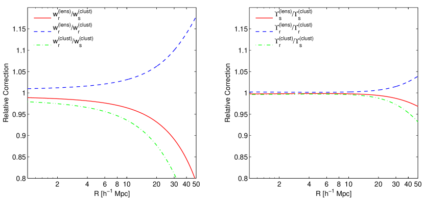
Figure 9 shows the correction terms for the bright LRG $(b=2.2)$ sample both for the projected correlation function $w$ and the ADSD $\Upsilon$. The integration length correction is shown as a blue dashed line. The window correction was obtained from comparing the linear theory predictions for $\Upsilon_{\text{gg,r}}^{\text{(\text{lens})}}$ and $\Upsilon_{\text{gg,r}}^{\text{(\text{clust})}}$. Again we see that the resulting corrections are much smaller for $\Upsilon$ than for $w$. This occurs for the same reason as discussed above in the context of redshift space distortions: by using a compensated window the sensitivity to long wavelength modes is removed and the limit $\chi_{\text{max}}\rightarrow\infty$ is approached faster, at which point the differences between different radial integration lengths disappear.

Figure 9 also shows the redshift factor as a green dash-dotted line and the final correction as a solid red line. The redshift correction is the inverse of the curve plotted in Fig. 8. We see that the projection length and redshift space effects go in the opposite direction. This partial cancellation further minimises their effect, so that for the ADSD $\Upsilon$, their combined effect is less than $3\%$ even at $R\approx 50\ h^{-1}\text{Mpc}$.

VII.3 Covariance matrix

Another benefit of the compensated ADSD is that its correlation matrix $\text{Corr}_{ij}=\left\langle\Upsilon_{i}\Upsilon_{j}\right\rangle/\sqrt{\left\langle\Upsilon_{i}\Upsilon_{i}\right\rangle\left\langle\Upsilon_{j}\Upsilon_{j}\right\rangle}$ has weaker off-diagonal contributions than that for the projected correlation function. Usually two point statistics such as the correlation function show strong correlations between different radial bins, i. e. important off-diagonal entries in the covariance matrix. The compensated window Eq. (17) relating the ADSD to the correlation function reduces these off-diagonal contributions remarkably. This statement refers to the cosmic variance contribution to the covariance matrix only. The shape noise adds predominantly to the diagonal error and thus further reduces the off-diagonals of the correlation matrix.

In Figure 10 we show columns extracted from the correlation matrices of $w$, $\Delta\Sigma$ and $\Upsilon$, respectively, for the bright LRG sample. The covariance matrix is estimated by calculating the variance over $160$ subvolumes of $750\times 750\times 300\ h^{-3}\text{Mpc}^{3}$. From this plot it is obvious that the off-diagonal contributions to the covariance matrix are reduced as one transitions from the projected correlation to the excess surface mass density and ADSD. One would expect some additional covariance due to the subtraction of $\Delta\Sigma(R_{0})$ in $\Upsilon$, but it turns out that the reduced off-diagonal covariance remains for the ADSD. We compare the signal-to-noise $(S/N)^{2}_{\Delta\Sigma}=\sum_{i,j}\Delta\Sigma_{i}C^{-1}_{ij}\Delta\Sigma_{j}$ and $(S/N)^{2}_{\Upsilon}=\sum_{i,j}\Upsilon_{i}C^{-1}_{ij}\Upsilon_{j}$, where $C$ are the covariance matrices of $\Delta\Sigma$ and $\Upsilon$, respectively. The sum runs over radial bins with $R_{i}>1\ h^{-1}\text{Mpc}$ for $\Delta\Sigma$ and $R_{i}>R_{0}$ for $\Upsilon$. We see that the signal-to-noise ratio is degraded by a factor $0.38<(S/N)_{\Upsilon}/(S/N)_{\Delta\Sigma}<0.45$ over a range of cutoff radii $5\ h^{-1}\text{Mpc}>R_{0}>1\ h^{-1}\text{Mpc}$. So the advantage of being able to interpret the result in terms of perturbation theory just has to be paid by a factor $2-3$ decrease in signal-to-noise.

VIII Variant Cosmologies

Figure 11: Cross-correlation coefficient of the ADSD $\Upsilon$ for the full galaxy sample. The panels show simulation output as circles with errorbars and theoretical predictions of Eq. (35) for $R_{0}=5\ h^{-1}\text{Mpc}$ (red solid lines). Top left panel: Reduced spectral index $n_{\text{s}}=0.95$ Top right panel: Increased normalisation $\sigma_{8}=0.9$ Bottom left panel: Reduced matter density $\Omega_{\text{m}}=0.2,\ \Omega_{\Lambda}=0.8$ Bottom right panel: Increased matter density $\Omega_{\text{m}}=0.3,\ \Omega_{\Lambda}=0.7$ We see that the increased number of high mass haloes in the $\Omega_{\text{m}}=0.3$ and $\sigma_{8}=0.9$ models leads to a higher number of satellite galaxies and thus partially compensates the drop of the cross-correlation coefficient for haloes on small scales.

Figure 12: Same as Fig. 12 but for the central LRGs. The central LRGs are a cleaner representation of a halo sample and thus better reproduce our theoretical expectations.

Figure 13: Same as Fig. 12, but for $R_{0}=3\ h^{-1}\text{Mpc}$ and for LRG sample from which the clusters with mass exceeding $M=3\times 10^{14}\ h^{-1}M_{\odot}$ and all satellites were removed. Due to the cluster subtraction the bias ratio changes to $\alpha=0.41$. In addition to the usual correction (red solid line) we also plot the phenomenological correction $r_{\text{cc}}\approx 1-\alpha^{2}\xi(R/2)/4$ (blue dashed line) The cluster subtraction also allowed us to reduce the cutoff radius to $R_{0}=3\ h^{-1}\text{Mpc}$.

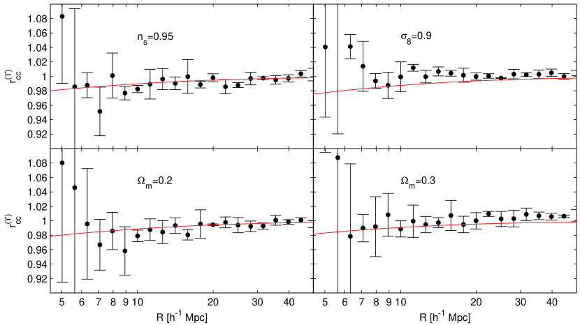
In the previous sections, we presented results for our mass clustering reconstruction for one specific cosmological model. In this section, we explore how well the $\Upsilon_{\text{mm}}$ reconstruction performs for four variations to our fiducial model.

The four variations are presented in Table 1, and we denote them by C1-C4. Each of these models differs from the fiducial model in exactly one parameter, and for each variation we have performed four simulations providing a volume of $V=13.5\ h^{-3}\ \text{Gpc}^{3}$. We populate these simulations using the same HOD parameters inferred for the luminosity-threshold LRG sample as described in §V.

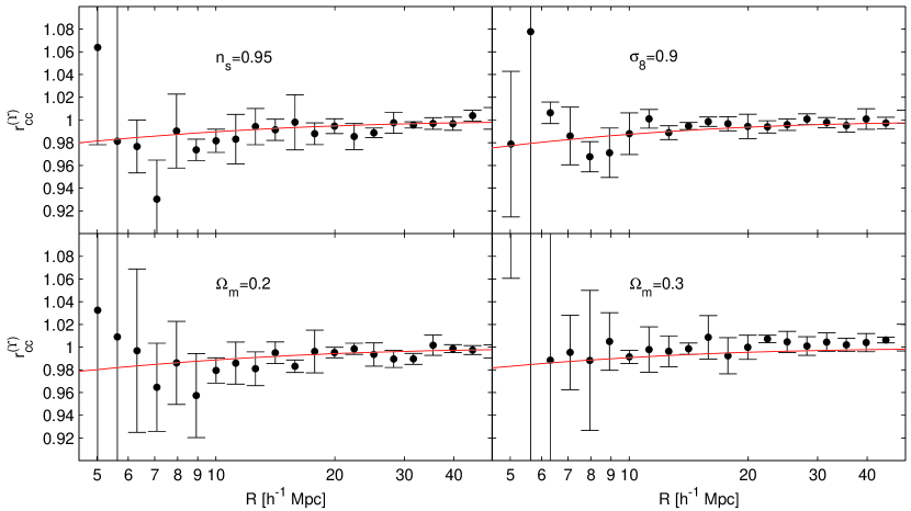
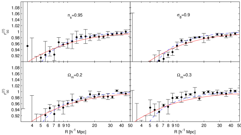
Figure 12 shows the cross-correlation coefficient inferred from the statistic $\Upsilon$, for $R_{0}=5\ h^{-1}\text{Mpc}$ for the full LRG sample. The reason for increasing the cutoff radius is that the cluster masses for some of the variant cosmologies are increased and thus we apply this more conservative cutoff radius to ensure $r_{\text{cc}}\approx 1$. We then see that the variation of cosmology does not significantly change the general trends observed for our fiducial model. We notice that there is a weak scale dependence, and in all cases the trend to lower $r_{\text{cc}}$ is well described by the theoretical model given by Eq. (43), which is over-plotted as a green line. There appears to be some small $(\sim 5\%)$ discrepancy for the higher $\sigma_{8}$ model at smaller scales $R<10\ h^{-1}\text{Mpc}$, where we see an increase in the cross-correlation coefficient. This is likely due to the fact that the cut-off scale $R_{0}$, is actually less than twice the virial radius of the most massive haloes, and so the statistics are still sensitive to the internal structure of the haloes.

We examined whether the agreement might be further improved through using only the central LRG galaxies in the reconstruction. The results of this test are presented in Figure 12, and we indeed find better agreement. We believe that this is due to the fact that the influence of satellite-satellite pairs from massive clusters has been removed. This means that the central galaxy sample is closer to a mass-selected halo sample and is thus less influenced by the details of how galaxies populate haloes.

A simple way to further reduce this sensitivity is to eliminate the most massive haloes from the data. Since these contain many galaxies, they are easy to identify in an observation. In Figure 13, we plot the cross-correlation coefficient of a halo sample, from which we removed all the clusters with mass exceeding $M\geq 3\times 10^{14}\ h^{-1}M_{\odot}$ and all the central galaxies. Having removed the clusters, we can lower the cutoff radius to $R_{0}=3\ h^{-1}\text{Mpc}$. Clearly the cross-correlation coefficient shows stronger deviations from unity. These are, however, better reproduced by our model than the full or central sample. To achieve this agreement we needed to change the bias ratio $\alpha$ accounting for the new upper mass threshold. The corrections in Figure 13 use $\alpha=0.41$ instead of our fiducial choice of $\alpha=0.26$.

Figure 14: Top panel: Reconstructed matter ADSD of the variant cosmologies for $R_{0}=5\ h^{-1}\text{Mpc}$. The points with errorbars show the simulation results for the four variant cosmologies as measured in the simulations, whereas the solid lines show the corresponding non-linear matter correlation function. From top to bottom: $\Omega_{\text{m}}=0.3$ (black stars), $\sigma_{8}=0.9$ (green squares), $n_{\text{s}}=0.95$ (red circles) and $\Omega_{\text{m}}=0.2$ (blue diamonds). The thick black line is the non-linear matter correlation function of our fiducial model plotted here for reference. Bottom panel: Fractional difference of the reconstructed matter statistics with respect to the fiducial model. From top to bottom we show $\Omega_{\text{m}}=0.3$ (solid black), $\sigma_{8}=0.9$ (green dotted), $n_{\text{s}}=0.95$ (red dash dotted) and $\Omega_{\text{m}}=0.2$ (blue dashed). For the $\Omega_{\text{m}}=0.2$ and $\Omega_{\text{m}}=0.3$ cosmologies we also include the effect of wrong a priori cosmology as thin lines with corresponding line style (for further discussion see text).

Another way to improve agreement between theory and simulation is to use a phenomenological correction factor. Inspired by the fact that the correction for the cross correlation coefficient $r_{\text{cc}}^{(\xi)}$ in Equation (31) is proportional to the correlation function, we can simplify our correction factor using the approximation $r_{\text{cc}}^{(\Upsilon)}(R)\approx 1-\alpha^{2}\xi(R/2)$/4. The argument $R/2$ in the correlation function can be motivated considering the window for the correlation function plotted in the right panel of Figure 2. There we see that the windows for $\xi(R/2)$ and $\Upsilon(R)$ peak at approximately the same scale in k-space. We over-plot the phenomenological correction as the red dashed line in Figure 13. With this replacement we can slightly improve the agreement between theory and measurement.

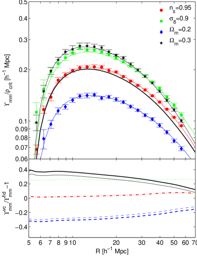
In Figure 14 we reconstruct the matter correlation $\Upsilon_{\text{mm}}(R)$ from the simulation measurements of $\Upsilon_{\text{gm}}(R)$ and $\Upsilon_{\text{gg}}(R)$ as the points with errorbars. For this plot we use the full galaxy samples, whose cross-correlation coefficient was shown in Figure 12. We see that the non-linear matter correlation function is reproduced for all the four variant cosmologies. Furthermore, there are clear differences both in shape and amplitude between the different cosmologies, so that inference of cosmological parameters should be feasible. Differences in $\Omega_{\text{m}}$ and $\sigma_{8}$ are more prominent than the effect of changing the slope of the primordial spectrum $n_{\text{s}}$. The small discrepancy between the simulations and the theoretical prediction for the high $\sigma_{8}$ model in Fig. 12 translates into a tension between inferred and real matter ADSD.

The lower panel of Figure 14 emphasises the possibility of inferring cosmological parameters by showing the fractional differences in the recovered ADSD for the different cosmologies C1 – C4 with respect to the fiducial model. Variations in the slope of the power spectrum differ from the fiducial model only on the $5\%$ level at $R=30\ h^{-1}\text{Mpc}$, whereas the quadratic dependence of the estimator on $\sigma_{8}\Omega_{\text{m}}$ leads to a clear separation of the variant $\sigma_{8}$ and $\Omega_{\text{m}}$ models from the fiducial model ($25\%$ at $R=30\ h^{-1}\text{Mpc}$). If the lensing study extends to sufficiently large scales $\sigma_{8}$ and $\Omega_{\text{m}}$ are separable by their shape. Here we are using the fact that a change in $\Omega_{m}$ or $\sigma_{8}$ affects the amplitude as well as the shape of the correlation function.

One caveat is that the inference of $\Upsilon_{\text{mm}}$ requires the assumption of an a priori cosmology. This assumption enters the reconstruction in three places. Firstly, we are using the clustering and lensing measurements as a function of the distance transverse to the line of sight. The observation, however, provides both clustering and tangential shear distortions as a function of angular separation. To relate the two, one needs to calculate the angular diameter distance to the foreground galaxy sample, which depends on $\Omega_{\text{m}}$. A wrong prior on the cosmological model would thus cause a horizontal shift in the inferred statistic. Secondly, the definition of the excess surface mass density includes the critical surface mass density, a ratio of the angular diameter distances to the lens, the source and between the two. The latter affects the amplitude of $\Upsilon_{\text{mm}}$ in quadrature. Thirdly, we use cosmology to compute the cross-correlation coefficient (Eq. 35). This also only has a weak dependence on cosmology, since the cross-correlation coefficient is close to unity to start with.

In order to estimate the magnitude of the first two effects we pose the following question: How is the inferred statistic for $\Omega_{\text{m}}=0.2$ or $\Omega_{\text{m}}=0.3$ affected if we wrongly assume the fiducial cosmology, $\Omega_{\text{m}}=0.25$, for the measurement? As a reasonable example, we take $z_{\text{l}}=0.25$ and $z_{\text{s}}=0.5$, for the lens and source redshifts. For these cases, we obtain a $2\%$ increase (decrease) in $\Sigma_{\text{crit}}$ for $\Omega_{\text{m}}=0.2$ ($\Omega_{\text{m}}=0.3$) with respect to the fiducial $\Omega_{\text{m}}=0.25$. These results are shown as the thin lines in the lower panel of Fig. 14. The shift caused by the cosmology dependence of the angular diameter distance to the lens galaxy has a smaller effect and is on the order of $\sim 1\%$. One route to remove part of this dependence from the measurement is to change the estimator $\Upsilon_{\text{mm}}\to\Upsilon_{\text{mm}}/\Sigma_{\text{crit}}^{2}$. This can be done by writing $\Upsilon_{\text{gm}}=\Sigma_{\text{crit}}\left[\overline{\gamma}_{\text{t}}(R)-R_{0}^{2}/R^{2}\gamma_{\text{t}}(R_{0})\right]$ and substituting this expression into Eq. (44)

$$\frac{\Upsilon_{\text{mm}}(R)}{\Sigma_{\text{crit}}(\Omega_{\text{m}})^{2}}=\frac{\left[\overline{\gamma}_{\text{t}}(R)-R_{0}^{2}/R^{2}\gamma_{\text{t}}(R_{0})\right]^{2}}{\Upsilon_{\text{gg}}(R)r_{\text{cc}}^{2}}\ .$$ (57)

The benefit of this redefinition is that the quantity we compare to theory has one cosmology dependence less, and $\Sigma_{\text{crit}}$ can be calculated for each tested cosmological model. However, the angular diameter distance still depends on $\Omega_{\text{m}}$. We could introduce another factor that takes care of this dependence, but for SDSS data at low redshift the effect is small. In general one can use an iterative procedure or check whether within the errors on $\Omega_{\text{m}}$ the effects exceed observational errors. A similar iterative procedure can be used to verify the sensitivity to the assumed value of the cross-correlation coefficient in the reconstruction.

Reconstruction Procedure

To conclude, we summarise our procedure for inferring the matter clustering from lensing and clustering measurements in terms of the following five steps:

1. Measure galaxy-galaxy lensing signal $\gamma_{\text{t}}$ for a certain lens galaxy sample, and calculate $\Delta\Sigma_{\text{gm}}(R)$ from the tangential shear. This first step requires the assumption of an a priori cosmological model that has to be confirmed or refuted by the final result.

2. Measure the galaxy-galaxy clustering of the lens galaxy sample and calculate the projected correlation function $w_{\text{gg}}(R)$. Integrate the result to obtain $\Delta\Sigma_{\text{gg}}(R)$.

3. Estimate the typical host halo virial radius of the galaxy sample under consideration. Use this estimated $R_{0}$ to correct for the central contributions in $\Delta\Sigma_{\text{AB}}(R)$ by calculating $\Upsilon_{\text{AB}}(R)=\Delta\Sigma_{\text{AB}}(R)-\Delta\Sigma_{\text{AB}}(R_{0})R_{0}^{2}/R^{2}$.

4. Make predictions for the transfer function and resulting matter auto-correlation functions for a set of cosmological parameters and/or modifications of gravity. Use these to calculate $\Upsilon_{\text{mm}}^{(\text{theo})}$ and find the best fit parameters by comparison to the empirical result.

5. Iterate until convergence.

IX Conclusions

In our study, we examined how well can one reconstruct the dark matter clustering from observations of galaxy clustering combined with galaxy-galaxy lensing. This reconstruction procedure could for instance be applied to the SDSS galaxy survey, in particular the Luminous Red Galaxies. In a first step, we generated realistic LRG galaxy catalogues for both a luminosity-threshold and a luminosity bin sub-sample of the LRGs. We then used these galaxy catalogues to extract information about the cross-correlation coefficient between galaxies and matter.

We introduced a new statistic $\Upsilon(R)$, which we termed the Annular Differential Surface Density (ADSD), that removes the influence of small, non-linear scales on the excess surface mass density. This subtraction is necessary since the scales smaller than the virial radius of the haloes are dominated by the halo profile rather than the pre-shell-crossing evolution of the large scale cosmological fluid. Both numerical studies and theoretical calculations indicate that the cross-correlation coefficient of the ADSD is close to unity and that the residual scale dependence is well described by an analytic correction. Having focused our investigations on the excess surface mass density $\Delta\Sigma_{\text{gm}}$, our results can be directly applied to measurements of galaxy-galaxy lensing and the projected galaxy correlation function.

We also studied systematic effects that might bias the comparison of lensing and galaxy clustering measurements. In terms of the projected correlation function, both numerical studies and a linear theory treatment, following Kaiser1987 , show that the common integration over $\pm 50\ h^{-1}\text{Mpc}$ along the line of sight is still biased by redshift space distortions. We have shown the necessity of correcting for the large scale peculiar motions in any such clustering measurement. We also investigated the effect of different window functions used for lensing and clustering. These introduce additional effects, that must be accounted for in the final analysis. We have found that the ADSD statistic $\Upsilon(R)$ is much less sensitive to both of the effects, and to long wavelength modes in general, than the usual projected correlation function $w(R)$, because of the (partially) compensated nature of its transverse window.

As our key result, we devised a method to recover the dark matter clustering from galaxy-galaxy lensing and galaxy clustering measurements using the cross-correlation coefficient for the ADSD. Assuming $r_{\text{cc}}=1$ for simplicity leads to at most $8\%$ bias on scales below $R\approx 5\ h^{-1}\text{Mpc}$ in the recovered statistic $\Upsilon_{\text{mm}}(R)$. We can however remove this bias based on our theoretical modelling of the scale dependence of the cross-correlation coefficient. The main advantage of our method is that the galaxy dependence is scaled out of the equations, since the theoretical model predictions for the cross-correlation coefficient between haloes and dark matter are relatively independent of the halo mass over a wide range of mass. Thus, we believe that the method devised here is more robust than the methods which are based on HOD fitting (e. g. Yoo2009 ), which fit for the cosmological parameters and the HOD parameters jointly, marginalising over the uncertainties in the HOD parameters.

A study on four other cosmological models verified the robustness of the new estimator. Varying one parameter of the fiducial $\Lambda$CDM model at a time, we found that the cross-correlation coefficient shows a scale dependence consistent with the fiducial model. We were able to reconstruct the ADSD of the matter correlation function, and the inferred statistic $\Upsilon_{\text{mm}}$ can be used to distinguish cosmological models both, from the shape and the amplitude of the recovered statistic. This study also showed that, if one is capable of accurately distinguishing central from satellite galaxies and/or remove clusters, then one can eliminate the influence of satellite galaxies and so render the cross-correlation coefficient closer to theoretical predictions for haloes in numerical simulations. These advantages make it worthwhile to define a clean central galaxy sample and to remove the clusters. While the non-linear matter correlation can be recovered with high fidelity, the linear correlation is only recovered at large scales. This fact strengthens the need for a well developed and tested perturbation theory of large-scale clustering that extends into the weakly non-linear regime and which can thus provide us with an estimator of $\xi_{\text{NL}}$ without having to carry out simulations for each cosmological model.

The ADSD statistic subtracts out a lensing signal at $R_{0}$ (Eq. 12). This subtraction procedure decreases the signal-to-noise on the inferred statistic $\Upsilon$ as compared to $\Delta\Sigma$. This price seems worth paying, since it brings the cross-correlation coefficient much closer to unity with residual deviations from unity that are well understood theoretically. An application of this method to observational data will have to address the problem of estimating $\Delta\Sigma(R_{0})$. The cubic spline fit used for our numerical studies will not be appropriate given the large statistical fluctuations in observed lensing signal. Several alternatives to estimate $\Delta\Sigma(R_{0})$ are explored in Mandelbaum2009 , with the most successful being a fit with a running power-law (three parameters) to the radial bins around $R_{0}$.

Our numerical results are based on the SDSS spectroscopic LRG sample, i. e. on the galaxies living in the most massive haloes. Based on the success and generality of the theoretical model we expect that a similar behaviour for the Main spectroscopic sample galaxies in the SDSS, which live predominantly in lower mass haloes. The lower halo masses may also enable a lower cutoff radius $R_{0}$, especially if haloes with higher mass are effectively removed from the sample. If the halo sample spans a wide range of masses, it should be split into mass bins and $R_{0}$ should be chosen appropriately for each of the mass bins. We shall reserve this topic for future investigation.