Quantum Chaotic Scattering in Microwave Resonators
Abstract
In a frequency range where a microwave resonator simulates a chaotic quantum billiard, we have measured moduli and phases of reflection and transmission amplitudes in the regimes of both isolated and of weakly overlapping resonances and for resonators with and without time-reversal invariance. Statistical measures for -matrix fluctuations were determined from the data and compared with extant and/or newly derived theoretical results obtained from the random-matrix approach to quantum chaotic scattering. The latter contained a small number of fit parameters. The large data sets taken made it possible to test the theoretical expressions with unprecedented accuracy. The theory is confirmed by both, a goodness-of-fit-test and the agreement of predicted values for those statistical measures that were not used for the fits, with the data.
pacs:
05.45.Mt,24.60.Ky,11.30.Er,85.70.GeIntroduction
Microwave resonators, also known as “microwave billiards”, are ideal systems to study properties of chaotic quantum systems Sto90 ; Sri91 ; Gra92 ; mw:chaos ; richter:playing . Most studies have focused on the statistical properties of eigenvalues and eigenfunctions, especially on tests of the Bohigas-Giannoni-Schmit BGS ; Boh84 ; heusler ; QC conjecture. According to that conjecture, the spectral fluctuation properties of quantum systems with chaotic classical dynamics coincide with those of random-matrix ensembles belonging to the same symmetry class. That statement holds up to level spacings determined by the period of the shortest periodic orbit of the system. We comment on that point below. Data are taken by coupling the resonators via one or several antennas to sources or sinks of a microwave power supply. Because of this arrangement, microwave resonators can also be viewed as open quantum systems, and measurements of the reflected and transmitted intensity amplitudes provide generic information on chaotic quantum scattering, each antenna acting as a single scattering channel scattering .
In this paper we report on measurements of the complex transmission and reflection amplitudes of chaotic microwave billiards, and on the theoretical analysis of such data. For the latter we use the generic approach to chaotic quantum scattering based on random-matrix theory (RMT). We have used two types of microwave resonators. In the first one, time-reversal () invariance holds and in the second one, it is violated by placing a magnetized ferrite within the cavity. The large set of scattering data taken with either device (considerably larger than data sets collected, for instance, in nuclear physics) allows us to test the RMT approach to chaotic scattering with unprecedented accuracy, both for systems that are invariant and for those that are not. Most experimental investigations of chaotic scattering have been restricted to measure cross sections rather than individual elements of the scattering matrix . In our setup we use a vector network analyzer to actually measure modulus and phase of the reflected and of the transmitted amplitudes and, thus, of individual -matrix elements. The additional information garnered in this way increases the significance of our tests. In addition to testing the RMT approach to chaotic scattering, we propose and test a method for the determination of the strength of violation from data on -matrix correlation functions. This is of particular significance for those chaotic quantum scattering systems for which the relevant parameters cannot be determined easily by dynamical calculations such as the semiclassical approximation Bluemel1998 . Some of our results have already briefly been reported in Refs. Friedrich2008 ; Schaefer2009 .
For -invariant systems statistical cross-section fluctuations have been thoroughly investigated experimentally and compared with theoretical predictions in the regime of isolated nuclear resonances Lyn68 (average resonance spacing very large compared to average resonance width ) and in the Ericson regime Ericson (), especially in nuclei Eri63 , but also in several other systems Blu88 ; Lawniczak2008 ; Schaefer2003 . We are not aware of similarly extended and precise tests of the RMT approach to chaotic scattering in the regime of weakly overlapping resonances (). Our work is intended to fill that gap. -invariance violation was tested in nuclear spectra Fre85 and for the Ericson regime in compound-nuclear reactions Ericson:66 ; mahaux:66 ; Witsch1967 ; Boose ; Harney90 . Upper bounds on the strength of the -invariance-violating interaction were deduced in both cases. -invariance violation caused by an external magnetic field has also been studied in electron transport through quantum dots Pluhar1995 and other devices Bergman and in ultrasound transmission in rotational flows Rosny . The RMT approach to -invariance violation Boose ; Pluhar1995 used in some of these papers is likewise tested very precisely in the present paper.
The theoretical approach to chaotic scattering is based on an expression for the -matrix originally derived in the context of nuclear physics mahaux:69 . That expression contains explicitly the Hamiltonian matrix of the system. Replacing the actual Hamiltonian by a -invariant random-matrix ensemble, one generates an ensemble of -matrices which describes generic features of chaotic scattering. Analytical expressions for the -matrix correlation functions of that ensemble which apply for all values of have been derived Ver85 . These are used in our analysis. Replacing the Hamiltonian by an ensemble of random matrices with partially broken invariance Pandey , one similarly generates an ensemble of -matrices that describes generic features of chaotic scattering with broken invariance. Some properties of that ensemble have been worked out previously Pluhar1995 ; Fyodorov2005 . To compare with our data we had to extend the theoretical results. This work is also reported in the present paper.
The paper is organized as follows. In Sec. I we describe the experimental setup and some typical results. In Sec. II we define the statistical measures in terms of -matrix elements and use these to analyze the data. In particular, we define a measure that quantifies the strength of -invariance violation. In Sec. III and in the Appendix we sketch the derivation of analytic expressions for the statistical measures. We use the method of Ref. Pluhar1995 . The theory contains a number of parameters. These are fitted to data. We test the theory with the help of a goodness-of-fit (GOF) test in Sec. IV.4. The basic assumption for the applicability of the GOF test is that the distribution of the Fourier-transformed -matrix elements are Gaussian and uncorrelated. In Sec. IV we demonstrate the validity of that assumption for chaotic scattering systems. In the case of -invariance violation, we test the theory further by comparing experimental values for the elastic enhancement factor and for the distribution of the diagonal -matrix elements with theoretical predictions based on parameter fits to other observables.
I Experiment
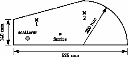
For an experimental study of universal fluctuation properties of chaotic scattering systems we used flat, cylindrical microwave resonators with the emitting and receiving antennas acting as single scattering channels. As long as the excitation frequency is chosen below , where is the height of the resonator and is the speed of light, only transverse magnetic TM0 modes can be excited, and the electrical field vector is perpendicular to the top and the bottom plates of the resonator. Then, the associated Helmholtz equation for the electric field strength is scalar and mathematically identical to the two-dimensional Schrödinger equation of a particle elastically reflected by the contour of the microwave resonator, i.e., of a quantum billiard Sto90 . The experiments were performed with resonators whose contour has the shape of a tilted stadium billiard Primack1994 . That shape was chosen to avoid bouncing-ball orbits. Each microwave resonator was constructed from three metallic plates. The bottom and the top of the resonator are formed by two 5 mm thick high-purity copper plates. The center plate had a hole in the shape of a tilted quarter stadium. The thickness of that plate determined the height of the resonator and differed for the two experiments. The quality factor Q increases with the height of the resonator. Thus, to ensure a high Q value the center plate for the -invariant case had a thickness of 14.6 mm (so that ). The plate was made of brass Friedrich2008 to technically permit the cutting-out of the hole. For the case with broken invariance a copper plate with a thickness of 5.0 mm, which coincided with the height of the ferrite described below, was used (so that ), see Ref. Schaefer2009 . In order to make sure that only TM0 modes are excited, the excitation frequency was actually chosen . Screws through the top, middle and bottom plates ensured the good electrical contact needed to achieve high-quality values of the resonator. Two thin wires (diameter about 0.5 mm) intrude 2.5 mm into the cavity through small holes (diameter about 2 mm) drilled into the lid of the resonator. They act as dipole antennas to couple the rf power into and out of the resonator. A vector network analyzer (VNA) provided the rf signal at a variable frequency and recorded the signal received at the same (other) antenna for reflection (transmission) measurements. The two signals were compared by the VNA in amplitude and phase to determine the complex-valued -matrix elements. These formed the data set for our analysis. The cavity is schematically shown in Fig. 1.
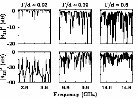
For a precise experimental determination of the elements of the -matrix all systematic and statistical errors must be minimized. The coaxial lines connecting the VNA with the cavity are the dominant source for systematic errors. They attenuate and reflect the rf signal. Both effects were removed by a proper calibration of the VNA. Systematic errors are also caused by the transmission properties of the two antennas. To account for these, the reflection spectrum of a small cylindrical resonator (diameter 5 mm, depth 20 mm) was measured using the same antenna geometry as in the actual experiment. The first resonance is located well above 30 GHz. Thus, in the frequency range of interest and for an ideal coupling of the antennas to the resonator all rf power would be reflected. Any deviation from this expectation was attributed to the antennas. The resulting correction was applied to the measured spectra in the actual experiments. The corrected values of the reflection and transmission spectra with the two antennas and provided the elements and of the complex -matrix as functions of the frequency . The frequency step size was . Typical measured reflection and transmission spectra are shown in Fig. 2. For the measurement of the -matrix element antenna 1 was used as emitting and receiving antenna, for that of antenna 2 was used as emitting, antenna 1 as receiving antenna, etc.. Figure 2 shows that at low excitation frequencies the resonances of the billiard are isolated, i.e. the mean resonance width and the correlation width , is small compared to the mean level spacing . Since it is a difficult if not impossible task to determine the resonance widths in the regime of overlapping resonances whereas the correlation width can be well estimated from the data using the Weisskopf formula Bla52 given in Eq. (28) below (for more details see Sec. III.2), we refer to the latter in the following.
As increases, so does the ratio , and the resonances begin to overlap.
The statistical errors of a single measurement caused by thermal fluctuations were reduced by an internal averaging routine of the VNA. The resulting errors were several orders of magnitude smaller than the signal and, thus, negligible. The data were analyzed in frequency intervals of GHz length yielding data points each. The limited number of statistically independent data points in every such frequency interval causes finite-range-of-data (FRD) errors. To increase the number of data points and to reduce the FRD errors Gibbs1965 ; Dallimore1966 , in some of the experiments a small scatterer (an iron disc, 20 mm diameter) was introduced into the microwave resonator (see Fig. 1) and moved to six different positions. We then speak of different realizations of the scattering system.
Experiments with violated invariance were done with a magnetized ferrite embedded within the resonator. Such induced Time-Reversal-Invariance Violation (TRIV) has been studied in numerous works So1995 ; Stoffregen1995 ; Wu1998 ; Hul2004 ; Schaefer2007 ; Schaefer2009 ; Vranicar . The ferrite has a cylindrical shape (4 mm diameter, 5 mm height), a saturation magnetization , and a linewidth , with 1 Oe=1000/4 A/m. It was provided by courtesy of AFT Materials GmbH (Backnang, Germany). Two NdFeB magnets (cylindrical shape, 20 mm diameter and 10 mm height) were placed outside the billiard at the position of the ferrite to provide the required magnetic fields perpendicular to the top and bottom plates of the resonator. The distance between the magnets and the ferrite could be adjusted by a screw thread mechanism, and field strengths of up to 360 mT could be achieved at the position of the ferrite. With this setup TRIV is induced via the following mechanism. Because of the external magnetic field the ferrite effectively acquires a macroscopic magnetization that precesses with the Larmor frequency around . This is the origin of the ferromagnetic resonance. The rf magnetic field inside the cavity is elliptically polarized and can be decomposed into two field components of opposite circular polarization with, in general, different amplitudes. Due to the Larmor precession of the magnetization the spins of the ferrite couple differently to the two magnetic field components. A reversal of time, simulated by an interchange of the input and output channels, swaps the rotational sense of the two field components and thus, due to their different amplitudes, effectively changes the coupling of the ferrite to the resonator mode. The induced TRIV is strongest if the frequency is close to that of the ferromagnetic resonance. The experiments with the embedded ferrite demanded a reduction of the height of the resonator to 5.0 mm, as the ferrite itself was only 5 mm in height.
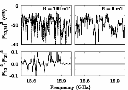
In a -invariant system, the scattering matrix is symmetric, . We refer to that property as reciprocity. Violation of reciprocity is the hallmark of TRIV. In the setup without ferrite the transmission spectrum for is indistinguishable from that for and reciprocity holds within the limits given by thermal noise (see left panels of Fig. 3). Typical transmission spectra of the billiard with ferrite and an external magnetic field of are shown in the right panel Fig. 3. The two graphs in the upper panels correspond to and , in the lower panel their difference is shown. Figure 3 demonstrates that reciprocity is violated.
II Statistical measures
In the present Section we define the statistical measures and use them to analyze the data. As pointed out in the Introduction, it is our aim to use the data for a detailed and accurate test of random-matrix theory. Our measures are tailored to this objective. They do not address properties of individual resonances but instead correlation properties of the fluctuating part of -matrix elements where and take either of the values and .
II.1 -Matrix Correlation Functions
We decompose the frequency-dependent -matrix into an average and a fluctuating part,
| (1) |
Here and in what follows, the angular brackets denote an average over a suitable frequency interval. In order to ensure a more or less constant coupling of the electric field modes to the antennas and to the walls of the resonator we have always used intervals of GHz length.
The autocorrelation function of is defined by
| (2) | |||||
This function quantifies the correlation between and at two different frequencies and . Figure 4 shows three examples of autocorrelation functions all obtained from data for the billiard without ferrite. The rate of decrease of the functions with increasing depends on the ratio . None of the functions has the Lorentzian shape predicted by Ericson Ericson for the regime of strongly overlapping resonances . We show later that the rate of decrease agrees with random-matrix predictions for the relevant values of .
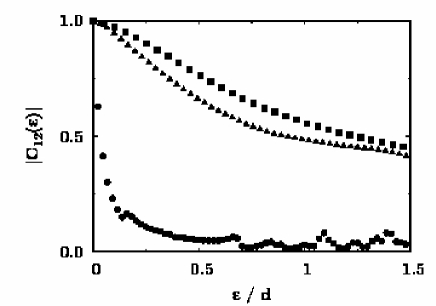
To quantify TRIV we measure the violation of reciprocity by the cross-correlation function of and ,
| (3) |
For a -invariant system, reciprocity holds, and . In case of complete TRIV we expect that and are completely uncorrelated, for all values of . (This expectation is borne out in Sec. III, see also Ref. Schaefer2007 for a treatment of the two-level case). In summary we have
| (4) |
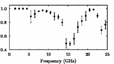
As explained in Sec. I, we have used six realizations to increase the statistical significance of the data. For each realization the cross-correlation coefficient was computed and the average over all realizations was taken. For an external magnetic field of 190 mT the resulting averaged cross-correlation coefficient is shown in Fig. 5. This coefficient deviates noticeably from unity around 6, 16 and 24 GHz, indicating TRIV. The first dip can be attributed to the ferromagnetic resonance which in our case is located at 6.6 GHz. We assume that the other two dips arise from an enhancement of the influence of the ferromagnetic resonance by standing rf magnetic fields inside the ferrite. Yet, the smallest values () obtained are well above zero. Hence, at a field strength of 190 mT the ferrite induces only a partial violation of invariance. This is also found at the other investigated field strengths up to 340 mT. In Sec. III we show that the strength of TRIV can be deduced from .
II.2 Fourier Transformation
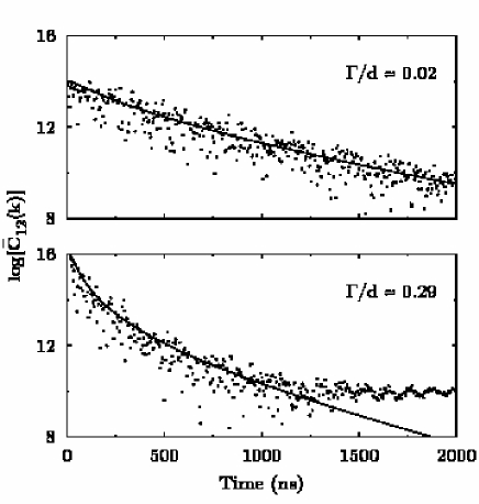
The measured scattering matrix elements are correlated for neighboring frequencies . The correlations result in a non-zero value of the autocorrelation function defined in Eq. (2) and depicted in Fig. 4. We show in Sec. IV.2 that after a Fourier transformation the correlations between data points at different times can be removed. This facilitates a statistically sound analysis and is our motivation for using that transformation. Since is measured at a discrete set of frequencies, the Fourier coefficients are likewise obtained at discrete time points , and the same is true of the autocorrelation function and its Fourier transform . Here, GHz is the length of the frequency interval and , see Section IV.1. We simplify the notation by using as argument of the Fourier transforms the integer . According to the Wiener-Khinchin theorem we have . Figure 6 shows two examples of at different values of for the -invariant system. The solid lines in Fig. 6 show a fit of the random-matrix expression defined in Sec. III to the data (the fit procedure is described in Sec. IV.1) and correspond to the local-in-time mean values of the Fourier coefficients. The data are seen to scatter about their time-dependent mean. In Sec. IV.2 it is shown that the data points divided by their local mean value at different times are indeed uncorrelated and that the distribution of the rescaled Fourier coefficients of the autocorrelation function is exponential. The decay of the average function (solid line in Fig. 6) is faster for (lower panel, frequency interval 9–10 GHz) than for (upper panel, frequency interval 3–4 GHz). This is due to stronger absorptive losses. In both cases the decay is non-exponential (and the autocorrelation function is, therefore, not Lorentzian). At and for times larger than about 1000 ns the decay is dominated by noise. Nevertheless, a decay over 5 orders of magnitude is experimentally well established.
II.3 Elastic Enhancement Factor
In chaotic scattering, elastic processes are known to be systematically enhanced over inelastic ones. The effect was first found in nuclear physics Satchler1963 ; EHK1969 ; Kretschmer1978 but plays a role also in mesoscopic physics Bergman . The enhancement depends on the degree of violation. The elastic enhancement factor is defined as
| (5) | |||||
where the second equality results from Eq. (2). In the limits of isolated resonances with many weakly coupled open channels and of strongly overlapping resonances the values for are Savin2006
| (6) |
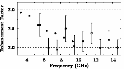
Here, for -invariant systems and for complete TRIV. The elastic enhancement factor was determined in two ways: (i) Using the first of Eqs. (5) we calculated the averages over frequency directly from the experimental values for . This amounts to determine from a single experimental value for each of the autocorrelation functions . (ii) In the second of Eqs. (5) we used the values of the autocorrelation functions obtained by a best fit of the analytical expression given in Eq. (26) below to the experimental one. These are the solid lines in Fig. 6. The method of fit (described in Sec. IV.1) uses the entire data set and is, therefore, expected to give more reliable values for . This is indeed borne out by the results shown in Figs. 7 and 8. For the -invariant case shown in Fig. 7 the elastic enhancement factor decreases from at low frequencies () to at high frequencies (), in qualitative agreement with Eq. (6).
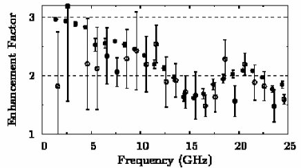
Results for the billiard with violated invariance are shown in Fig. 8. Although was obtained from a data set of 6 realizations, the values obtained with method (i) still show large uncertainties while method (ii) yields reliable results. Again displays an overall decrease from to with increasing . However, at frequencies of about 6, 16 and 24 GHz dips are observed. Around 16 and 24 GHz the values of drop below 2. This is not possible for a -invariant system. These features are similar to those of the cross-correlation coefficient in Fig. 5. Both measures indicate a substantial violation of -invariance at about 6, 16 and 24 GHz.
III Theory
As stated in the Introduction, it is the aim of the experiments reported and analyzed in this paper to test random-matrix theory as applied to chaotic scattering systems. According to the Bohigas-Giannoni-Schmit conjecture Boh84 , the spectral fluctuation properties of chaotic -invariant quantum systems coincide with those of the Gaussian orthogonal ensemble [GOE], those of quantum systems with complete TRIV with those of the Gaussian unitary ensemble [GUE] of random matrices. Systems with partial violation of invariance are accordingly described by a crossover from orthogonal to unitary symmetry. For such systems, analytical expressions for central statistical measures of scattering processes (i.e., the autocorrelation function (2) and the cross-correlation coefficient (3)) have not been worked out before. We fill that gap in Sec. III.1.
III.1 Crossover from Orthogonal to Unitary Symmetry: the Autocorrelation function and the Cross-Correlation Coefficient
For chaotic scattering processes, the GOE GUE crossover was extensively investigated in Ref. Pluhar1995 . There the destruction of weak localization by an external magnetic field in the transmission of electrons through a few-channel disordered microstructure was determined. The connection between the conductance and the -matrix is given by the Landauer formula,
| (7) |
where counts the total number of open channels and an equal number of incoming and outgoing channels is assumed. Efetov’s supersymmetry method Efetov was used to calculate ensemble averages of squares of -matrix elements for . The -matrix embodies the GOE GUE crossover in the manner described below. Here we describe the extension of that approach to the calculation of the autocorrelation function (2) and the cross-correlation coefficient (3). These observables were not considered in Ref. Pluhar1995 .
We write the unitary scattering matrix in the general form mahaux:69
| (8) |
where the inverse propagator is given by
| (9) |
The matrix elements and describe the coupling of antennas and with the resonator mode Schaefer2007 . The sum over in Eq. (9) extends over the two antennas but includes also a number of fictitious channels. The latter describe Ohmic absorption in the cavity Schaefer2003 . The matrix is the Hamiltonian of the closed billiard. It has dimension and the limit is eventually taken.
The coupling matrix elements are chosen real, for all , and a violation of invariance by an external magnetic field is taken into account only in . We also assume that the are independent of frequency . That assumption holds within frequency intervals of GHz width. The experiment was designed such that direct power transmission between the antennas is excluded so that the average -matrix is diagonal. We have verified that fact experimentally. A diagonal average -matrix is implied by the relation
| (10) |
The parameter measures the average strength of the coupling of the resonances to channel . The Hamiltonian is a member of a random-matrix ensemble describing partial violation of invariance. In random-matrix theory, the GOE GUE crossover is written as Pandey
| (11) |
The real and symmetric matrix is a member of the GOE, and the elements of the real and antisymmetric matrix are uncorrelated Gaussian-distributed random variables. Thus,
| (12) |
Here has the dimension energy and for the GOE denotes half the radius of Wigner’s semicircle. The parameter measures the strength of -invariance violation. For the matrix is a member of the GUE. However, on the local level (energy intervals measured in units of the mean level spacing of the GOE) the transition from GOE to GUE already takes place when the typical matrix element of the TRIV term becomes comparable to , i.e. when
| (13) |
or when . The -matrix (8) is symmetric only for , and reciprocity does not hold for .
Starting with Eq. (1) we have used angular brackets to denote the running average over (parts of) the experimental spectra. The averages were actually taken over 1 GHz frequency intervals. Now we consider an ensemble of -matrix elements of the form of Eq. (8) obtained by inserting many realizations of the random Hamiltonian in Eq. (11). We denote averages over that ensemble also by angular brackets. This is legitimate because ergodicity guarantees the equality of ensemble average and of the running average over a single realization of the ensemble, see Sec. II C3 of HWM2009 .
The autocorrelation function for the -matrix defined in Eq. (8) is known for the case of invariance () Ver85 , for the case of complete TRIV () Fyodorov2005 and had to be calculated for the case of partial TRIV (). For the first case it reads
| (14) | |||||
The upper index of indicates that an average over the GOE was taken. The integration measure is given by
| (15) | |||||
and we have
| (16) | |||||
Here and in Eqs. (19) and (24) below the input parameters are the mean level spacing and the transmission coefficients in all channels , defined as
| (17) |
We observe that . For all three cases the matrix elements occur in the final expression for the correlation functions only via the transmission coefficients. Using the analytical result for Ver85 and Eq. (10) one finds that
| (18) |
The choice of the parameters is described in Section IV.1. The threefold integrals in Eq. (14) and in Eq. (24) below are numerically computed most conveniently in terms of the integration variables introduced in Ref. Verbaarschot1986 .
For the second case, the -matrix autocorrelation function was worked out in Ref. Fyodorov2005 ,
| (19) | |||||
The upper index of now indicates the average over the GUE.
In our experiments we deal with partial TRIV, i.e. with the third case and the -matrix autocorrelation function had to be calculated for all values of the parameter introduced in Eq. (11). To this end we generalized the work of Ref. Pluhar1995 . We present here only the result and defer details to the Appendix. The autocorrelation function is given in terms of a threefold integral over integration variables and , see Eq. (2) of Ref. Gerland1996 . However, the integrals are evaluated numerically more conveniently in terms of the integration variables given in Sec. 5 of Ref. Verbaarschot1986 . For the transformation to these one needs to distinguish in the integrations over and the case where and the case where . For instance, for the case the transformation to integration variables is given by
| (20) |
where
Then both, the -matrix autocorrelation function and the cross-correlation coefficient are obtained as special cases of a function . With the notations
| (21) |
and
| (22) | |||||
| (23) | |||||
the function reads
| (24) | |||||
Here,
The integration measure and the function are given explicitly in Eqs. (15) and Eq. (16). Setting () in Eq. (24) yields the autocorrelation function (the cross-correlation coefficient),
| (26) | |||||
| (27) |
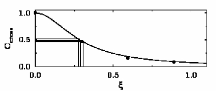
We observe that for , i.e. , the function defined in Eq. (III.1) vanishes and in Eq. (24) turns into the autocorrelation function of the GOE given in Eq. (14). We checked our analytical results by comparison with RMT simulations. In Fig. 9 we show the cross-correlation coefficient versus as obtained analytically and by RMT simulation for a typical set of transmission coefficients. We also indicate how the analytical result is used to determine the value of from a measured value of the cross-correlation coefficient. To test the validity of Eq. (24) we compare in Figs. 10 and 11 analytic results for the autocorrelation functions with numerical simulations, both in the frequency and in the time domains. The parameter measures absorption and is defined in Sec. III.2 below. In all cases, the agreement is very good.

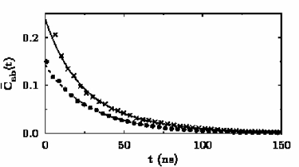
The theoretical expressions given in Eqs. (14), (19) and (24) are obtained as averages over the ensemble of Hamiltonian matrices defined in Eq. (11) in the limit and directly yield the autocorrelation function. In contrast, Fig. 4 shows autocorrelation functions obtained by averaging the data in a frequency interval of GHz width. For conceptual clarity we distinguish both cases by referring to the theoretical and to the experimental autocorrelation functions, respectively.
III.2 Parameters
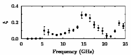
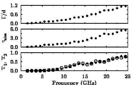
The parameters in Eqs. (14), (19) and (24) are the average level spacing , the transmission coefficients for all channels , and the parameter for TRIV. We have calculated from the Weyl formula Bal76 . A starting value for the parameter was determined from the experimental cross-correlation coefficients shown in Fig. 5 as described in the caption of Fig. 9. Here we use that the cross-correlation coefficient depends only weakly on the transmission coefficients in the frequency range 1–25 GHz. Results are shown in Fig. 12.
The largest value of is . In determining by fitting the theoretical expressions for the autocorrelation function to the data, we also use as fit parameter, with starting value as just described. For the channels and , i.e. for the antennas, we also have determined starting values from the definition Eq. (17) and from the measured values of and . The fits discussed in Sec. IV yielded , within 5 % of these starting values. The remaining transmission coefficients describe Ohmic absorption in the walls of the resonator and the ferrite. If for all absorbing channels, the products over these channels appearing in Eqs. (14), (19) and (24) simplify so that each of the three theoretical autocorrelation functions depends only on the sum of the transmission coefficients for the absorbing channels. Accordingly, in addition to , and the parameter was used as fitting parameter. To estimate the correlation width of the resonances, we have used the Weisskopf formula Bla52
| (28) |
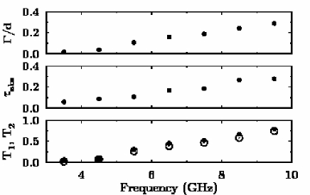
and the fitted values for , , and . Using numerical simulations and with help of the analytic result Eq. (14) for the autocorrelation function we checked that this formula indeed yields a very good estimate for the correlation length even in the regime of weakly overlapping resonances and for a few open channels. The results of our fits (each done in a frequency interval of GHz length) are displayed in Figs. 13 and 14. We show as obtained from Eq. (28) (top panel), (middle panel) and and (bottom panel) versus frequency for the case without and with TRIV, respectively. The transmission coefficients and generally increase with frequency. We note that without the ferrite never exceeds the value (regime of weakly overlapping resonances) since the excitation frequency must be chosen below GHz, whereas in the system with ferrite we have GHz and thus attains values as large as .
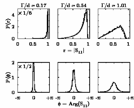
III.3 Distribution of -Matrix Elements
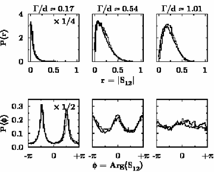
The distribution of -matrix elements is not known completely in analytical form, neither for the -invariant system nor for TRIV. The most complete information is available in the regime of strongly overlapping resonances (). In a basis in channel space where is diagonal, the inelastic -matrix elements with have a bivariate Gaussian distribution Aga75 . Thus the phase of is uniformly distributed in the interval . The distribution function of the modulus depends only on the ratio and is given by
| (29) |
The diagonal elements have a bivariate Gaussian distribution only for and only if . Otherwise, unitarity constraints cause the distribution to differ from the Gaussian form Dav88 ; Dav89 ; Dietz2009a .
In Ref. Fyodorov2005 an analytic expression for the distribution of the elastic elements of the scattering matrix of a generic chaotic system without or with partially violated invariance was derived. It applies for cases with many open channels. With the notation
| (30) |
the distribution of is given by
| (31) | |||||
With the help of the transformation Eq. (20), the definitions (23) and with the analytic expression for the function given in Ref. Fyodorov2005 may be cast into the form
For -invariant systems the threefold integral can be simplified, and takes the form
| (33) | |||||
Here, for and otherwise, is the number of open channels and
| (34) | |||||
The corresponding functions with index 2 are given by the same expression except that the integration limits have to be replaced by .
These analytic results were previously tested experimentally for the case of a single open channel plus absorption in Refs. Mendez2003 ; Kuhl2005 ; Hul2005 ; Lawniczak2008 ; HarmInv . In Fig. 15 we compare for several frequency intervals the experimental distributions of the elastic -matrix element with the theoretical predictions for the case of two open channels with absorption. The data were taken with the billiard used for the experiments with partial TRIV but without the ferrite. This was done because that billiard has a smaller height so that the range where only a single vertical mode is excited, extends up to GHz. Higher values of the frequency result in larger absorption and in larger values of . It is here that the theoretical result (33) is expected to apply. The value of was determined from the Weisskopf formula given in Eq. (28) and from the values of obtained from a fit of the Fourier transform of the -matrix autocorrelation function as described in Sec. IV. The very good agreement corroborates the precision of the fitting procedure and of the GOF test discussed below. Note that the distributions are very far from a bivariate Gaussian distribution.
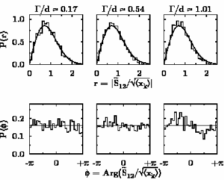
An analytic expression for the distribution of the off-diagonal elements of the -matrix exists in the Ericson regime , however not in the range of achieved in the experiments. In Fig. 16 we, therefore, compare experimental distributions to RMT simulations. We note again the good agreement. In the frequency range 23–24 GHz (where ) the distribution of is well described by Eq. (29), and the distribution of the phases is nearly uniform. Thus, in this frequency range the distribution of the non-diagonal -matrix elements is already close to that expected in the Ericson regime while that of the diagonal elements is still far from Gaussian.
IV Data Fits and Distribution of Fourier Coefficients
In the present Section we test predictions of random-matrix theory with the experimental data. We proceed as follows. Using the results of Sec. II.2, we fit the parameters of the Fourier transforms of the theoretical expressions for the autocorrelation functions (Eqs. (14) and (24)) to the data. We show that within the accuracy of the data and after rescaling, the distribution of the Fourier-transformed -matrix elements is Gaussian. This property is used to develop a goodness-of-fit (GOF) test that quantitatively tests the quality of RMT predictions. As a second test of RMT we compare predicted values of the elastic enhancement factors with the data.
In Sec. III.3 we have shown that the real and imaginary parts of the -matrix elements in general do not have a Gaussian distribution. How can this fact be reconciled with the statement just made that the Fourier-transformed -matrix elements do have such a distribution? The Fourier transform is a linear transformation, after all. We answer that question as we proceed.
IV.1 Fits
We focus attention on the fluctuating part of the -matrix elements (see Eq. (1)) and omit the indices and for brevity. By definition we have . Data are taken at frequency increments . The mean level spacing , the transmission coefficients and , and the absorption coefficient are typically constant in frequency intervals of GHz width. In every such interval we have measured values of for all combinations of channel indices . We write where is the frequency at the lower end of the interval and . We use discrete Fourier transformation and define
| (35) |
so that
| (36) |
We fit the parameters in the theoretical expressions (14) and (24) to the distribution of the squares of these Fourier coefficients. The Wiener-Khinchin theorem states that the latter are equal to the Fourier coefficients of the experimental autocorrelation functions . We accordingly calculate the Fourier transforms of the theoretical autocorrelation functions in Eqs. (14) and (24) at the same discrete values of as occur in the discrete Fourier transformation in Eq. (35). The parameters are the transmission coefficients , , and . For the transmission coefficients and we used Eq. (17) with experimental values for and as starting points but allowed the values of and to vary. The best-fit values differed by no more than % from the starting values. For a starting value was obtained from a comparison of the experimental and the analytic cross-correlation coefficients as outlined in Sec. III.2. For the fit parameter no starting values could be computed from the measured data. The fit yields the solid lines shown in Fig. 6 and defines . We observe that decreases by several orders of magnitude over the available range of values. We also observe that for the Fourier coefficients and are uncorrelated. This follows from the fact that the autocorrelation functions depend only on the difference of the two frequency arguments and is shown below in Eq. (39).
As stated in the Introduction, the use of generic expressions derived from RMT is justified only for energy spacings bounded from above by the period of the shortest periodic orbit in the classical microwave billiard. Therefore, Fourier coefficients are generic only for times larger than the repetition time of the shortest periodic orbit We have estimated that time and found it to be smaller than the time-index of in Eq. (35). We note, however, that the average -matrix elements (which correspond to ) are not generic. This is mirrored by the fact that these are used as input parameters in our analysis.
IV.2 Gaussian Distribution
We ask: How are the distributed about their mean values determined by the fits? In order to study the distribution of the and of the coefficients with good statistics, we must sample all data points shown in Fig. 6. To this end we remove the strong and systematic dependence by rescaling: We divide by and by and find that the renormalized -matrix elements have a bivariate Gaussian distribution both for the elastic (case shown in Fig. 17) and the inelastic one (shown in Fig. 18). The left-hand side of Fig. 19 shows that after rescaling of the the logarithms of the rescaled coefficients scatter about zero. Moreover we find that the distribution of the is stationary in . By this we mean that the distribution of the determined from sampling their values within some interval of length does not depend on the choice or length of that interval. The statistical accuracy of that statement is obviously limited by the fact that the number of data points contained in the interval decreases with decreasing length . Stationarity allows us to study the joint distribution function of all obtained from -matrix data that lie within a frequency interval of length GHz. That step improves the statistical accuracy of the result.
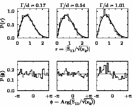
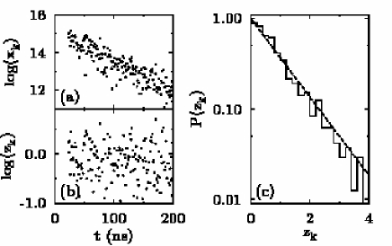
The right-hand side of Fig. 19 shows that the coefficients have an exponential distribution, as expected for the absolute squares of variables with a bivariate Gaussian distribution. To test this statement quantitatively we observe that for an exponential distribution the ratio should have the value two. For our finite data set we define
| (37) |
and obtain for the variance of
| (38) |
Evaluation of that ratio for the data set in the range 16–17 GHz shown in Fig. 19 with 6 realizations gives , which is within the defined error limits () for the contributing data points. A systematic analysis of our data ensemble for all frequency intervals between and GHz yields 13 accepted and 11 rejected ratios, i.e. 54 % of all frequency intervals are within the 1- range defined by Eq. (38). In the range 10–25 GHz the acceptance ratio increases to 80 %. This is well above the expected 1- value of approximately .
IV.3 Analysis
The results displayed in Fig. 19 are puzzling. The elements of are correlated over a frequency range . They do not follow a Gaussian distribution. There are non-trivial higher-order correlations. On the other hand, there exists no discernible correlation among the rescaled Fourier coefficients , and these are consistent with a bivariate Gaussian distribution for . How is it possible that a non-Gaussian distribution becomes Gaussian after Fourier transformation and rescaling?
We first show that rescaling removes binary correlations. For simplicity, we do so for the case of a continuous frequency ranging over the entire real axis. For clarity, we distinguish the ensemble average (indicated by an overbar) from the running average over the spectrum of a single realization (indicated by angular brackets).
Without rescaling, the distribution of would obviously not be Gaussian. Moreover, rescaling does indeed remove all correlations between pairs of -matrix elements. To see this, we calculate the correlation function of two Fourier-transformed -matrix elements, using the translational invariance of the two–point correlation function [ for all real ]. That gives
| (39) |
The Fourier transform of determines only the average value of ; pairs of Fourier-transformed -matrix elements with different arguments are uncorrelated. We Fourier-transform back to the frequency domain and find that the correlation function of a pair of Fourier-back-transforms is a delta function in frequency. Thus, the binary correlation has been removed by rescaling. Put differently, we may consider the quantities as Fourier transforms of -matrix elements that are pairwise uncorrelated.
Correlations of higher order (involving more than two –matrix elements) imply correlations of higher order of the elements of and of . Such correlations are not removed by rescaling. But they are made irrelevant by the way in which the distribution of the is sampled. That is done by considering the index as a label only. Any relation to the time scale originally inherent in the Fourier transformation is lost. We simply order the by size, asking how many occur in each size interval. That yields the distribution in Fig. 19. The dependence on is scrambled. It is not possible from that distribution to reconstruct correlations that may have existed among its elements.
These arguments do not explain why the distribution of is Gaussian. (For that we must resort to the law of large numbers). But they show why correlations that are known to exist among the do not prevent a Gaussian to emerge for the distribution of the .
IV.4 Goodness-of-Fit Test
To test the quality of the fit of the theoretical autocorrelation functions in Eqs. (14) and Eq. (24) to the data, we developed a goodness-of-fit test. The test applies to uncorrelated data with an exponential distribution. As shown in Sec. IV.3 that condition is met by the rescaled experimental Fourier coefficients . We recall that the mean values are determined by fitting a small number of parameters. This renders the decision non-trivial whether the fit is compatible with the data. As a measure for the goodness of the fit we used the expression
| (40) |
which quantifies the difference between the data points and the best-fit value for the theoretical expressions. The quantity is non-negative and vanishes exactly if for all . The expression Eq. (40) is a generalization of the test used for Gaussian data, see Chaps. 14 and 16 of Ref. Harney2003 . If has an exponential distribution then the distribution of is given by
| (41) |
For our test we approximated by a chi-squared distribution with degrees of freedom
| (42) |
Here, is the expectation value of and is given by
| (43) |
where is Euler’s constant. The agreement between and is better than 2 %. The same measure was used for a goodness-of-fit test in Ref. Friedrich2008 .
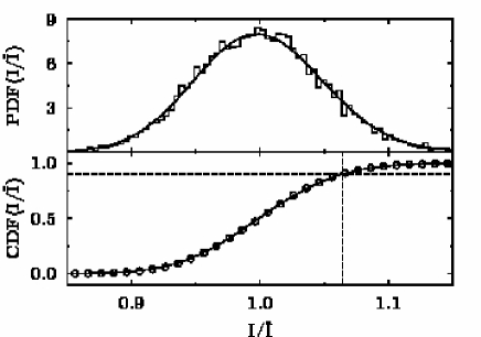
The test procedure is illustrated in Fig. 20. Upon the definition of a certain threshold (in the Figure: ) on the cumulative distribution function a limit is obtained (in the Figure: ) which may not be exceeded by if the GOF test is to accept the model. The limit is defined by
| (44) |
The value of quantifies the confidence into the test in the sense that is the probability to make a wrong decision by rejecting a valid theory. We choose .
In the fitting procedure the Fourier transforms of the theoretical autocorrelation functions of the GOE (Eq. (14)), of the GUE (Eq. (19)), and for the case of partial -invariance violation (Eq. (26)), respectively, were fitted to the experimental Fourier coefficients. One example of such a fit is shown in Fig. 21. In the upper four panels the results are compared to the data (dots) in the frequency domain. The lower panel shows the experimental Fourier coefficients (dots) together with the best fits of the GOE (solid) and the partial TRIV (dash-dotted) result.
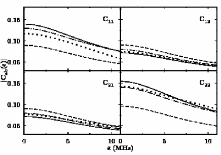
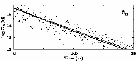
We observe that the experimental Fourier coefficients scatter widely around their average; the scatter is too large to directly arrive at a conclusive decision using the GOF test described above. Therefore data were taken from a total of six different realizations of the experiment. Moreover, the theoretical curves lie very close to each other. This corroborates the need of a goodness-of-fit test. This GOF test in conjunction with the enlarged data basis leads to the decision that within the confidence threshold only the expression for partial TRIV describes the data. The GOE and GUE expressions are ruled out.
V Summary
We have measured reflection and transmission amplitudes in chaotic microwave billiards with two antennas. The measurements were performed in the regimes of isolated and of weakly overlapping resonances. Both a -invariant system and a system with partially violated invariance were investigated. The latter was realized by placing a magnetized ferrite within the microwave billiard. The measurements yielded the moduli and phases of all four elements of the scattering matrix in a range of frequencies limited by the requirement that only one vertical mode be excited in the billiard. The frequency range was divided into intervals of 1 GHz width. Within each interval, statistical measures for -matrix fluctuations like the Fourier transform of the -matrix autocorrelation function, the distribution of -matrix elements, or the elastic enhancement factor were determined from the data.
We compared the results with theoretical expressions based on random-matrix theory. For -invariant systems and for systems with full violation of invariance these were given in Refs. Ver85 ; Pluhar1995 ; Fyodorov2005 while for systems with partial -invariance violation they had to be calculated. This was done by extending the existing supersymmetry approach. The parameters of the theory are the transmission coefficients and for the two antennas, the parameter describing absorption in the billiard, and the parameter for the strength of -invariance violation. Starting values for these were partly obtained directly from the data, but final values were always determined from fits of the RMT expressions to some of the experimental measures.
The large data sets taken made it possible to test the theoretical expressions with unprecedented accuracy. The outcome of these tests is recapitulated in Table 1. In particular, we used the following stringent tests.
(i) Goodness-of-fit (GOF) test. For the -invariant system, that test accepted the fit of the theoretical result for the Fourier-transformed autocorrelation function to the experimental data in all 1 GHz intervals. In the case of -invariance violation, the GOF test was applied to data fits of RMT expressions for all three cases, i.e., the one for -invariant systems, the one for systems with complete and the one for systems with partial -invariance violation. The results of these fits are summarized in Table 1. The fit is accepted in just 7 frequency intervals for the first case, it is rejected in all but two intervals for the second case, and it is accepted in all but one interval for the third case. In each 1 GHz window the fitted values of agree with the values determined in Sec. III.2. We conclude that the GOF test is a powerful tool to uncover the small effects of partial -invariance violation on -matrix fluctuation properties.
| (GHz) | 1 | 2 | 3 | 4 | 5 | 6 | 7 | 8 | 9 | 10 | 11 | 12 |
|---|---|---|---|---|---|---|---|---|---|---|---|---|
| no TRIV | ||||||||||||
| TRIV | ||||||||||||
| partial |
| (GHz) | 13 | 14 | 15 | 16 | 17 | 18 | 19 | 20 | 21 | 22 | 23 | 24 |
|---|---|---|---|---|---|---|---|---|---|---|---|---|
| no TRIV | ||||||||||||
| TRIV | ||||||||||||
| partial |
(ii) We inserted the fitted parameters into theoretical expressions for the distribution of the diagonal -matrix elements and, in the case of violation, for the elastic enhancement factor. The results agreed well with the data. To the best of our knowledge, this is the first time that the elastic enhancement factor as function of the parameter has been investigated in such detail over such a large frequency range.
As an additional test, we extended our measurements beyond the frequency range where only one vertical electric mode in the resonator is excited. When two such modes are excited, the resonator does not simulate a quantum billiard. The fit of the theoretical result based on random-matrix theory to the experimental data is rejected by the GOF test. That was shown in Ref. Friedrich2008 and is not reproduced here. We have numerically simulated the -matrix correlations for that case under the assumption that the two modes of vertical excitation do not interact, using for the random Hamiltonian ensemble sets of real symmetric matrices consisting of two diagonal blocks. Such matrices are commonly used to mimic spectral properties of -invariant chaotic systems with some underlying symmetry. It was shown in Ref. Friedrich2008 that our simulations qualitatively reproduce the experimental autocorrelation function. The failure of the GOF test shows that our testing procedure is sensitive to the existence of such symmetries.
We conclude that the theoretical expressions for the -matrix correlation functions, for the distribution of -matrix elements, and for the elastic enhancement factor based on random-matrix theory, are in excellent agreement with data measured on chaotic microwave billiards, both for the -invariant case and for the case with partial -invariance violation. Our work constitutes the most stringent test of the statistical theory of quantum chaotic scattering yet done. The success in the case of partial -invariance violation shows that the strength parameter can be determined reliably from scattering data. This is important in cases where that parameter cannot be reliably obtained theoretically from a dynamical calculation like, for instance, the semiclassical approximation. The largest achieved values for the -invariance violation strength parameter equals 0.3. Numerical calculations show that for this value the spectral fluctuations of the Hamiltonian for the closed resonator defined in Eq. (11) almost coincide with those of the GUE Bohigas1995 . We also found that for they do not differ significantly from those presented in Ref. So1995 , where the conclusion was drawn, that complete breaking is achieved. However, even for the value of is still far from zero. This shows that is a particularly suitable measure of the strength of violation.
Acknowledgements.
We would like to thank J. Verbaarschot for his initial help concerning the analytic description of systems with -violation. Moreover we would like to thank D. Savin and Y. Fyodorov for discussions on the distribution of the -matrix elements. F. S. is grateful for the financial support from the Deutsche Telekom Foundation. This work was supported by the DFG within SFB 634.Appendix
For the derivation of the analytic expressions for the autocorrelation function and the cross correlation coefficient in Eqs. (24), (26) and (27), we used Efetov’s supersymmetry approach in the form of Ref. Pluhar1995 . Due to the symmetry-breaking term in Eq. (11), the integration over the Grassmann variables which involves determining terms of highest (in our case eighth) order in the anticommuting variables, is rather difficult. In Ref. Pluhar1995 the integration was done with Efetov’s original parametrization for the integration measure and a method first developed in Ref. Altland1992 . The starting point was the generating functional
| (45) | |||||
Here, Detg and Trg denote the graded determinant and trace as defined in the supersymmetry formalism of Ref. Ver85 . The inverse propagator and the matrix are matrices. Introducing the matrix
| (46) |
we have for the inverse propagator
| (47) |
Here and with and is the diagonal supermatrix that distinguishes between the advanced () and retarded () parts of . The index denotes the commuting, the anticommuting components. The quantity equals the difference of the arguments of the -matrix elements and . The matrix is given as
| (48) |
where the matrix with entries
| (49) |
is the projector onto the block. With Eq. (8) we obtain
| (50) |
where denotes the trace over the index of the resonator modes, and it can be checked that
| (51) |
Averaging over the ensemble becomes feasible when we write the generating functional as a Gaussian superintegral
| (52) |
over an eight-dimensional supervector . The matrices and have been extended to supermatrices,
| (53) |
and
| (56) | ||||
| (59) |
where and are the parts of that are symmetric and antisymmetric in the indices and , respectively. The indices in Eq. (52) arise due to the doubling of dimension. The eight-component supervector is given in terms of the four-component supervector and its adjoint , where as
| (60) |
The symmetrized form of the autocorrelation function, , is obtained by choosing the plus sign, that of the unnormalized cross-correlation coefficient by setting and choosing the minus sign in
| (61) |
Ensemble averaging over the Hamiltonian of the generating functional Eq. (52) yields
| (62) |
where
| (63) |
with the supermatrix and . The matrix is eight-dimensional. It results from the doubling of dimension, . The quartic dependence of on is eliminated with help of a Hubbard-Stratonovich transformation. After expanding the resulting exponent in the large limit in the small quantities and the remaining integral reads
| (64) |
where and with (c.f. Eq. (10))
| (65) |
Here, trg denotes the supertrace over the indices , and Trg includes the summation over the level index . The supermatrix contains the commuting and the Grassmannian integration variables. For the integration Efetov’s original parametrization of the matrix was used.
Before performing the integration needs to be differentiated twice with respect to and at and for , c.f. Eq. (61). Only terms of second order in and survive. Since is linear in , these are obtained from the second order term in of which equals with . Then we finally obtain (see Eq. (61))
| (66) |
For the integration over the Grassmann variables, we proceeded as in appendix B of Ref. Pluhar1995 . The result is a threefold integral. For arbitrary values of the transmission coefficients , the expression for the autocorrelation function for the case is obtained from that given in Eq. (2) of Ref. Gerland1996 by including in the integrand the factor arising for non-vanishing from the last term in the first line of Eq. (65). Here, are the integration variables. It is straightforward to compute the autocorrelation function for the case by proceeding as in appendix B of Pluhar1995 . The result for the cross-correlation coefficient is obtained by multiplying the second and the third rectangular bracket in Eq. (2) of Gerland1996 by . All this yields for the autocorrelation function and the cross-correlation coefficient the expressions given in Eqs. (24), (26) and (27).
References
- (1) H.-J. Stöckmann and J. Stein, Phys. Rev. Lett. 64, 2215 (1990).
- (2) S. Sridhar, Phys. Rev. Lett. 67, 785 (1991).
- (3) H.-D. Gräf, H. L. Harney, H. Lengeler, C. H. Lewenkopf, C. Rangacharyulu, A. Richter, P. Schardt, and H. A. Weidenmüller, Phys. Rev. Lett. 69, 1296 (1992).
- (4) C. Dembowski, H.-D. Gräf, A. Heine, R. Hofferbert, H. Rehfeld, and A. Richter, Phys. Rev. Lett. 84, 867 (2000); C. Dembowski, B. Dietz, T. Friedrich, H.-D. Gräf, A. Heine, C. Mejía-Monasterio, M. Miski-Oglu, A. Richter, and T. H. Seligman, Phys. Rev. Lett. 93, 134102 (2004); R. Hofferbert, H. Alt, C. Dembowski, H.-D. Gräf, H. L. Harney, A. Heine, H. Rehfeld, and A. Richter, Phys. Rev. E 71, 046201 (2005); C. Dembowski, B. Dietz, T. Friedrich, H.-D. Gräf, H. L. Harney, A. Heine, M. Miski-Oglu, and A. Richter, Phys. Rev. E 71, 046202 (2005).
- (5) A. Richter: Playing Billiard with Microwaves - Quantum Manifestations of Classical Chaos, in Emerging Applications of Number Theory, 109, The IMA Volumes in Mathematics and its Applications, Ed.: D. A. Hejhal, J. Friedmann, M. C. Gutzwiller and A. M. Odlyzko (Springer, New York, 1999), S. 479.
- (6) G. Casati, F. Valz-Gris, and I. Guarneri, Lett. Nuovo Cimento 28, 279 (1980), M.V. Berry, Ann. Phys. (N.Y.) 131, 163 (1981).
- (7) O. Bohigas, M. J. Giannoni, and C. Schmit, Phys. Rev. Lett. 52 1 (1984).
- (8) S. Heusler, S. Müller, A. Altland, P. Braun, and F. Haake, Phys. Rev. Lett. 98, 044103 (2007).
- (9) H.- J. Stöckmann, Quantum Chaos - An Introduction, (Cambridge University Press, Cambridge, 1999); F. Haake, Quantum Signatures of Chaos, 2nd edition, (Springer Verlag, Berlin 2001); Chaos and Quantum Physics, edited by M.-J. Giannoni, A. Voros, and J. Zinn-Justin (Elsevier, Amsterdam,1991).
- (10) S. Albeverio, F. Haake, P. Kurasov, M. Kuś, and P. Šeba, J. Math. Phys. 37, 4888 (1996); F. Haake, M. Kuś, P. Šeba, H.-J. Stöckmann, and U. Stoffregen, J. Phys. A 29, 5745 (1996); H.-J. Stöckmann and P. S̆eba, J. Phys. A 31, 3439 (1998); X. Zheng, T. M. Antonsen, and E. Ott, Electromagnetics 26(1), 3 (2006); B. Dietz, A. Heine, A. Richter, O. Bohigas, and P. Leboeuf, 035201R (2006).
- (11) R. Blümel and U. Smilansky, Phys. Rev. Lett. 60, 477 (1988).
- (12) B. Dietz, T. Friedrich, H. L. Harney, M. Miski-Oglu, A. Richter, F. Schäfer, and H. A. Weidenmüller, Phys. Rev. E 78, 055204(R) (2008).
- (13) B. Dietz, T. Friedrich, H. L. Harney, M. Miski-Oglu, A. Richter, F. Schäfer, J. Verbaarschot, and H. A. Weidenmüller, Phys. Rev. Lett. 103, 064101 (2009).
- (14) J. E. Lynn, The Theory of Neutron Resonance Reactions (Clarendon Press, Oxford, 1968).
- (15) T. Ericson, Phys. Rev. Lett. 5, 430 (1960).
- (16) T. E. O. Ericson and T. Mayer-Kuckuk, Ann. Rev. Nucl. Sci. 16, 183 (1966); A. Richter, in: Nuclear Spectroscopy and Nuclear Reactions, Part B, ed. J. Cerny, 343 (Academic Press, New York, 1974).
- (17) R. Blümel and U. Smilansky, Phys. Rev. Lett. 60, 477 (1988); G. Stania and H. Walther, Phys. Rev. Lett. 95, 194101 (2005); J. Madronero and A. Buchleitner, Phys. Rev. Lett. 95, 263601 (2005); G. L. Celardo, F. M. Izrailev, V. G. Zelevinsky, and G. P. Berman, Phys. Rev. E 76, 031119 (2007).
- (18) M. Lawniczak, O. Hul, S. Bauch, P. Šeba, and L. Sirko, Phys. Rev. E 77, 056210 (2008).
- (19) R. Schäfer, T. Gorin, T. H. Seligman, and H.-J. Stöckmann, J. Phys. A 36, 3289 (2003).
- (20) J. B. French, V. K. B. Kota, A. Pandey, and S. Tomsovic, Phys. Rev. Lett. 54, 2313 (1985).
- (21) T.E.O. Ericson, Phys. Lett. 23, 97 (1966).
- (22) C. Mahaux and H. A. Weidenmüller, Phys. Lett. 23, 100 (1966).
- (23) W. von Witsch, A. Richter, and P. von Brentano, Phys. Rev. Lett. 19, 524 (1967); E. Blanke, H. Driller, W. Glöckle, H. Genz, A. Richter, and G. Schrieder, Phys. Rev. Lett. 51, 355 (1983).
- (24) D. Boosé, H. L. Harney, and H. A. Weidenmüller, Phys. Rev. Lett. 56, 2012 (1986); Z. Phys. A 325, 363 (1995).
- (25) H. L. Harney, A. Hüpper, and A. Richter, Nucl. Phys. A 518, 35 (1990).
- (26) Z. Pluhař, H. A. Weidenmüller, J. A. Zuk, C. H. Lewenkopf, and F. J. Wegner, Ann. Phys. 243, 1 (1995).
- (27) G. Bergman, Phys. Rep. 107, 1 (1984).
- (28) J. de Rosny, A. Tourin, A. Derode, P. Roux, and M. Fink, Phys. Lett. 95, 074301 (2005).
- (29) C. Mahaux and H. A. Weidenmüller, Shell Model Approach to Nuclear Reactions (North Holland, Amsterdam, 1969).
- (30) J. J. M. Verbaarschot, H. A. Weidenmüller, and M. R. Zirnbauer, Phys. Lett. 149B, 263 (1984); Phys. Rep. 129, 367 (1985).
- (31) A. Pandey, Ann. Phys. (N.Y.) 134, 110 (1981).
- (32) Y. V. Fyodorov, D. V. Savin, and H.-J. Sommers, J. Phys. A: Math. Gen. 38, 10731 (2005).
- (33) H. Primack and U. Smilansky, J. Phys. A 27, 4439 (1994).
- (34) W. R. Gibbs, Phys. Rev. 139, B1185 (1965).
- (35) P. J. Dallimore and I. Hall, Nucl. Phys. 88, 193 (1966).
- (36) J. M. Blatt and V. F. Weisskopf, Theoretical Nuclear Physics, Wiley and Sons, New York, 1952.
- (37) P. So, S. M. Anlage, E. Ott, and R. N. Oerter, Phys. Rev. Lett. 74, 2662 (1995).
- (38) U. Stoffregen, J. Stein, H.-J. Stöckmann, M. Kuś, and F. Haake, Phys. Rev. Lett. 74, 2666 (1995).
- (39) D. H. Wu, J. S. A. Bridgewater, A. Gokirmak, and S. M. Anlage, Phys. Rev. Lett. 81, 2890 (1998).
- (40) O. Hul, S. Bauch, P. Pakonski, N. Savytskyy, K. Zyczkowski, and L. Sirko, Phys. Rev. E 69, 056205 (2004).
- (41) M. Vranic̆ar, M. Barth, G. Veble, M. Robnik, and H.-J. Stöckmann, J. Phys. A 35, 4929 (2002).
- (42) B. Dietz, T. Friedrich, H. L. Harney, M. Miski-Oglu, A. Richter, F. Schäfer, and H. A. Weidenmüller, Phys. Rev. Lett. 98, 074103 (2007).
- (43) H. P. Baltes and E. R. Hilf, Spectra of Finite Systems, Wissenschaftsverlag, Mannheim, 1976.
- (44) G. R. Satchler, Phys. Lett. 7, 55 (1963).
- (45) J. Ernst, H. L. Harney, and K. Kotajima, Nucl. Phys. A 136, 87 (1969).
- (46) W. Kretschmer and M. Wangler, Phys. Rev. Lett. 41, 1224 (1978).
- (47) H. A. Weidenmüller and G. Mitchell, Rev. Mod. Phys. 81, 539 (2009).
- (48) D. V. Savin, Y. V. Fyodorov, and H. J. Sommers, Acta Phys. Pol. A 109, 53 (2006), proceedings of the 2nd Workshop on Quantum Chaos and Localisation Phenomena, Warsaw, Poland, May 19-22.
- (49) K. B. Efetov, Adv. Phys. 32, 53 (1983).
- (50) J. J. M. Verbaarschot, Ann. Phys. (N.Y.) 168 368 (1986).
- (51) U. Gerland and H. A. Weidenmüller, Europhys. Lett. 35, 701 (1996).
- (52) D. Agassi, H. A. Weidenmüller, and G. Mantzouranis, Phys. Rep. 22 (1975) 145.
- (53) E. D. Davis and D. Boosé, Phys. Lett. B 211, 379 (1988).
- (54) E. D. Davis and D. Boosé, Z. Physik A 332, 427 (1989).
- (55) B. Dietz, H. L. Harney, A. Richter, F. Schäfer, and H. A. Weidenmüller, Phys. Lett. B, in press.
- (56) R. A. Méndez-Sánchez, U. Kuhl, M. Barth, C. H. Lewenkopf, and H.-J. Stöckmann, Phys. Rev. Lett. 91 174102 (2003).
- (57) U. Kuhl, M. Martínez-Mares, R. A. Méndez-Sánchez, and H.-J. Stöckmann, Phys. Rev. Lett. 94 144101 (2005).
- (58) O. Hul, O. Tymoshchuk, S. Bauch, P. M. Koch, and L. Sirko, J. Phys. A 38 10489 (2005).
- (59) U. Kuhl, R. Höhmann, J. Main, and H.-J. Stöckmann, Phys. Rev. Lett. 100, 254101 (2008).
- (60) F. M. Dittes, H. L. Harney, and A. Müller, Phys. Rev. A 45, 701 (1992).
- (61) H. L. Harney, F. M. Dittes, and A. Müller, Ann. Phys. (N.Y.) 220, 159 (1992).
- (62) H. L. Harney, Bayesian Statistics — Parameter Estimation and Decisions, Springer Verlag, Heidelberg, 2003.
- (63) O. Bohigas, M. J. Giannoni, A. M. Ozorio de Almeida, and C. Schmit, Nonlinearity 8, 203 (1995).
- (64) A. Altland, S. Iida, A. Müller-Groeling, and H. A. Weidenmüller, Ann. Phys. 219, 148 (1992).