Universal power laws in the threshold network model:
A theoretical analysis based on extreme value theory

Abstract

We theoretically and numerically investigated the threshold network model with a generic weight function where there were a large number of nodes and a high threshold. Our analysis was based on extreme value theory, which gave us a theoretical understanding of the distribution of independent and identically distributed random variables within a sufficiently high range. Specifically, the distribution could be generally expressed by a generalized Pareto distribution, which enabled us to formulate the generic weight distribution function. By using the theorem, we obtained the exact expressions of degree distribution and clustering coefficient which behaved as universal power laws within certain ranges of degrees. We also compared the theoretical predictions with numerical results and found that they were extremely consistent.

1 Introduction

Many researchers during the last decade have enthusiastically investigated the structure of real networks that have emerged from various disciplines, such as information science, sociology, and biology. As a result of these investigations, some have found two features inherent in their networks, i.e., small-world [1] and scale-free [2], which were vastly different from those of the regular and random networks already known. The term “small-world” means that the clustering coefficient remains large and that there are very short paths between every two nodes, and “scale-free” means that the degree distribution has a long tail, which usually obeys a power law. All networks having both (or either) of these are often called complex networks. Many physicists have tried to theoretically understand their features by using mathematical models.

The threshold network model is a non-growing network model that explains the properties of complex networks. Each node in this model has an intrinsic weight that is randomly distributed according to a certain probability distribution function. Every pair of nodes satisfying the condition that the sum of their weights is over a certain given threshold is linked. When the weights are generated from various types of restricted distribution (specifically, exponential or power-law type distributions), both the degrees of nodes and the degree-wise clustering coefficient obey universal power laws at the high tails of the degrees [3, 4, 5]. We investigated the scale-free feature for both the degrees and clustering coefficient in a wider variety of weight distribution functions using extreme value theory[6, 7, 8]. Extreme value theory provides an explanation of the distribution of independent and identically distributed (iid) random variables within a sufficiently high range. According to this theory, the distribution is universally expressed with a generalized Pareto distribution (GPD). This gives the expression of a generic weight distribution function, which finally results in universal power laws, which is the main contribution of this paper.

This paper is organized as follows. We briefly explain the threshold network model in Sec. 2, then give the formulas for the distributions of degrees and clustering coefficient. In Sec. 3, we briefly review extreme value theory. We present the theoretical results of universal power laws in Sec. 4 and compare the theory with numerical results in Sec. 5. We finally conclude with a summary and a discussion in Sec. 6.

2 Threshold Network Model

First, we will explain the threshold network model [3, 4, 5] with $n(>1)$ nodes. We assign a weight, $w_{i}\ (1\leq i\leq n)$, to each node by using an iid random variable from a certain weight distribution function, $f(w)$. When the sum of two weights $w_{i},w_{j}$ ($i\neq j$) in every pair of nodes is more than or equal to a given threshold, $\theta$, i.e.,

$$w_{i}+w_{j}\geq\theta.$$ (1)

an edge is formed between them. Going through this procedure, we can finally obtain a threshold network.

Let

$$F(w)=\int_{-\infty}^{w}f(w^{\prime})dw^{\prime}$$ (2)

be a weight function. Here, we assumed that the threshold network had a large number of nodes, $n$. From the definition of the threshold network, nodes with the same weight values have an equal number of degrees, and the degrees of nodes monotonically increase as their weight values increase. Due to these features, the degree of the threshold model is specifically described in the continuous limit of $n$ as

$$k=n\int_{\theta-w}^{\infty}f(w^{\prime})dw^{\prime}=n\{1-F(\theta-w)\},$$ (3)

where $0\leq k\leq n$. This equality gives a one-to-one correspondence between the degree, $k$, and the weight, $w$. Using Eq. (3), the degree distribution, $p(k)$ ($0\leq k\leq n$), naturally follows

$$p(k)\equiv f(w)\frac{dw}{dk}=\frac{f\biggl{(}\theta-F^{-1}\biggl{(}1-\frac{k}{n}\biggr{)}\biggr{)}}{nf\biggl{(}F^{-1}\biggr{(}1-\frac{k}{n}\biggr{)}\biggr{)}}.$$ (4)

The degree-wise clustering coefficient, $C(k)$, means that the clustering coefficient of nodes with degree $k$ also leads to

$$C(k)\equiv \frac{1}{k(k-1)}\biggl{\{}\int_{w}^{\infty}dw^{\prime}nf(w^{\prime})\int_{\theta-w}^{\infty}dw^{\prime\prime}nf(w^{\prime\prime})$$

$$+\int_{\theta-w}^{w}dw^{\prime}nf(w^{\prime})\int_{\theta-w^{\prime}}^{\infty}dw^{\prime\prime}nf(w^{\prime\prime})\biggl{\}}$$

$$= \frac{n^{2}}{k(k-1)}\biggl{\{}-1+2\frac{k}{n}+\biggl{(}1-\frac{k}{n}\biggr{)}F\biggl{(}\theta-F^{-1}\biggl{(}1-\frac{k}{n}\biggr{)}\biggr{)}$$ (5)

$$-\int_{n[1-F(\theta-F^{-1}(1-\frac{k}{n}))]}^{k}\biggl{(}1-\frac{k^{\prime}}{n}\biggr{)}p(k^{\prime})dk^{\prime}\biggr{\}}.$$

3 Extreme Value Theory

Next, let us review the essence of extreme value theory. This theory mathematically treats the statistical behavior of the maximum

$$M_{n}=\max\{X_{1},\cdots,X_{n}\},$$ (6)

where $X_{i}$ ($1\leq i\leq n$) is an ensemble of iid random variables given by a common distribution function, $F(x)$. In a linearly renormalized maximum, there exists the following limit distribution

$$G(z)=\exp\left\{-\left[1+\xi\left(\frac{z-\mu}{\sigma}\right)\right]^{-1/\xi}\right\},$$ (7)

where $z$ is defined as $\{z:1+\xi(z-\mu)/\sigma>0\}$, $-\infty<\mu<\infty$ is a location parameter, $\sigma>0$ is a scale parameter, and $-\infty<\xi<\infty$ is a shape parameter. This is called a distribution of generalized extreme values (GEVs). Note that the GEV distribution includes three statistical distributions: Fréchet ($\xi>0$), Gumbel ($\xi=0$), and (reversed, meaning $x\to-x$) Weibull ($\xi<0$). As listed in Table 1, the maxima of various types of distribution function converge to a GEV distribution (for more details, see pp. $153$–$157$ in Embrechts et al. [6]).

Table 1: Relation between types of distribution function $F(x)$ and shape parameter $\xi$.

Name	Distribution Function $F(x)$	Shape Parameter $\xi$
Beta	$\frac{\Gamma(a+b)}{\Gamma(a)\Gamma(b+1)}\int_{0}^{x}x^{\prime a-1}(1-x^{\prime})^{b-1}dx^{\prime},$	$-1/b$
	$0<x<1,\ \ a,b>0$.
Uniform	$x,\ \ \ \ \ 0<x<1.$	$-1$
Exponential	$1-\exp(-\lambda x),\ \ \ \ \ x>0,\ \ \lambda>0.$	$0$
Normal	$\int_{-\infty}^{x}\frac{1}{s\sqrt{2\pi}}\exp\{-(x^{\prime}-m)^{2}/2s^{2}\}dx^{\prime},$	$0$
	$-\infty<x<\infty,\ \ -\infty<m<\infty,\ \ s>0$.
Lognormal	$\int_{0}^{x}\frac{1}{S\sqrt{2\pi}}\exp\{-(\ln x^{\prime}-M)^{2}/2S^{2}\}dx^{\prime}/x^{\prime},$	$0$
	$x>0,\ \ -\infty<M<\infty,\ \ S>0$.
Pareto	$1-x^{-\alpha},\ \ \ \ \ x>1,\ \ \alpha>0.$	$1/\alpha$

It is well known in extreme value theory that the following theorem is satisfied using $G(x)$.

Theorem 1

Assume that the sample maxima of $F(x)$ converge to $G(x)$. Then, for sufficiently large $u$, a distribution function $H$ of $Y=X-u$, conditional on $X>u$, yields

$$H_{u}(y) \equiv \textrm{Pr}\{X\leq y+u\ |\ X>u\}$$ (8)

$$= \frac{F(u+y)-F(u)}{1-F(u)}\sim 1-\left(1+\frac{\xi y}{\tilde{\sigma}}\right)^{-1/\xi},$$

on $\{z:1+\xi y/\tilde{\sigma}>0\}$, where $\tilde{\sigma}=\sigma+\xi(u-\mu)$.

The last equality in Eq. (8) is called a generalized Pareto distribution (GPD). For details of the proof, see pp. $76$–$77$ in Coles [7] or pp. $10$–$11$ in de Haan and Ferreira [8].

We rearrange Eq. (8) with respect to $F(x)$, where $x=y+u$. It then follows that

$$F(x) = (1-F(u))H_{u}(x-u)+F(u),$$ (9)

$$\sim 1-(1-F(u))\left(1+\frac{\xi(x-u)}{\tilde{\sigma}}\right)^{-1/\xi},$$

for $x\geq u$. Here, assume $F(x)$ in Eq. (9) is a weight distribution function of the threshold network in Eq. (2). Then, Eq. (9) represents a generic weight distribution function under the conditions where the number of nodes $n$ and the lower bound, $u$, in Eq. (9) are sufficiently large.

4 Main Results

4.1 Degree Distribution

To calculate the degree distribution in Eq. (4) with the generic weight function in Eq. (9), we first need to derive $f(x)$ and $F^{-1}(1-k/n)$. The former can easily be calculated by differentiating Eq. (9) :

$$f(x)\equiv F^{\prime}(x)=\frac{1-F(u)}{\tilde{\sigma}}\left(1+\frac{\xi(x-u)}{\tilde{\sigma}}\right)^{-\frac{1}{\xi}-1},$$ (10)

for $x\geq u$. The latter can also be calculated by using Eqs. (3) and (9). Rearranging Eq. (3) with respect to $\theta-w$, we have

$$F^{-1}\left(1-\frac{k}{n}\right)=\theta-w.$$ (11)

Here, substituting Eq. (9) with $x=\theta-w\ (\geq u)$ into Eq. (3), it follows that

$$\frac{k}{n} = 1-F(\theta-w)$$ (12)

$$= (1-F(u))\left(1+\frac{\xi}{\tilde{\sigma}}(\theta-w-u)\right)^{-\frac{1}{\xi}},$$

where $\theta-w\geq u$. Rearranging the last equality in Eq. (12) with respect to $\theta-w$, and then substituting this resulting equation into the right-hand side of Eq. (11), it follows that

$$F^{-1}\left(1-\frac{k}{n}\right)=\frac{\tilde{\sigma}}{\xi}\left\{\left(\frac{k/n}{1-F(u)}\right)^{-\xi}-1\right\}+u.$$ (13)

Therefore, by using Eqs. (10) and (13), the degree distribution of the generic weight function is finally given by

$$p(k)=\frac{1}{n}\left[\left\{2+(\theta-2u)\frac{\xi}{\tilde{\sigma}}\right\}\left(\frac{k/n}{1-F(u)}\right)^{\xi}-1\right]^{-\frac{1}{\xi}-1}.$$ (14)

As we can see from Eq. (14), the degree distribution obeys a power law, $p(k)\sim k^{-(1+\xi)}$ when $\xi\neq 0$. For $\xi=0$, the distribution becomes

$$p(k) = d(k)\exp\{-c(k)\},$$ (15)

$$\to \frac{n(1-F(u))^{2}\exp\left\{-\frac{\theta-2u}{\tilde{\sigma}}\right\}}{k^{2}}\sim k^{-2},$$

for $\xi\to 0$, where

$$c(k) = \frac{1}{\xi}\ln\left[\left\{2+(\theta-2u)\frac{\xi}{\tilde{\sigma}}\right\}\left(\frac{k/n}{1-F(u)}\right)^{\xi}-1\right],$$

$$d(k) = \frac{1}{n}\left[\left\{2+(\theta-2u)\frac{\xi}{\tilde{\sigma}}\right\}\left(\frac{k/n}{1-F(u)}\right)^{\xi}-1\right]^{-1}.$$

To summarize, we analytically obtain the universal power law for the range of large degree,

$$p(k) \sim k^{-(1+\xi)}\hskip 14.22636pt(\xi\neq 0),$$ (16)

$$\sim k^{-2}\hskip 31.29802pt(\xi=0).$$ (17)

Here, note that Eqs. (10) and  (12) that we used to obtain the power law are satisfied for $x\geq u$ and $\theta-w\geq u$, respectively. Therefore, the applicable range of weight in the power law is given by

$$u\leq w\leq\theta-u.$$ (18)

Equivalently, that of degrees is also obtained by using Eq. (3)

$$n\{1-F(\theta-u)\}\leq k\leq n\{1-F(u)\}.$$ (19)

These inequalities indicate the applicable range of degree-distribution scales with the number of nodes, $n$. To keep the inequalities in Eq. (18) unbroken, threshold $\theta$ must satisfy $\theta\geq 2u$, where $u$ is sufficiently large. This indicates that we have to implicitly assume a high threshold to universally observe the power laws.

4.2 Clustering Coefficient

We next calculate the clustering coefficient in Eq. (5) with the generic weight function in Eq. (9). This automatically means that the clustering coefficient is also restricted in the range of Eqs. (19) and  (18), resulting in a high threshold. First, we need to check whether the lower bound of the integral range in Eq. (5) is within the range in Eq. (19). Using Eqs. (11) and  (18), it follows that

$$n\left[1-F\left(\theta-F^{-1}\left(1-\frac{k}{n}\right)\right)\right] = n\{1-F(w)\}$$

$$\geq n\{1-F(\theta-u)\},$$

This means that the lower bound is inside the domain in Eq. (19), and therefore the integral can successfully be calculated without violating the requirements of extreme value theory. Combining Eqs. (9) and  (13), it follows that

$$F\left(\theta-F^{-1}\left(1-\frac{k}{n}\right)\right)=1-(1-F(u))D,$$ (20)

where

$$D=\left\{2+\frac{\xi}{\tilde{\sigma}}(\theta-2u)-\left(\frac{k/n}{1-F(u)}\right)^{-\xi}\right\}^{-\frac{1}{\xi}}.$$ (21)

Therefore, the clustering coefficient is given by

$$C(k) = \frac{n^{2}}{k(k-1)}\left\{\frac{k}{n}-\left(1-\frac{k}{n}\right)(1-F(u))D\right.$$

$$-\left.\int_{n(1-F(u))D}^{k}\left(1-\frac{k^{\prime}}{n}\right)p(k^{\prime})dk^{\prime}\right\},$$

$$\sim k^{-1},$$

for large $k$, where $p(k)$ is the same as in Eq. (14). When $\xi=0$, Eq. (20) with Eq. (21) can be explicitly calculated as

$$F\left(\theta-F^{-1}\left(1-\frac{k}{n}\right)\right)$$

$$=1-\frac{(1-F(u))^{2}n\exp\left\{-\frac{\theta-2u}{\tilde{\sigma}}\right\}}{k}.$$ (23)

When $\xi=0$, therefore,

$$C(k) = \frac{n^{2}}{k(k-1)}(1-F(u))^{2}\exp\left(\frac{2u-\theta}{\tilde{\sigma}}\right)$$ (24)

$$\times\left(1+\frac{\theta-2u}{\tilde{\sigma}}+2\log\frac{k}{n(1-F(u))}\right),$$

$$\sim k^{-2}.$$

To sum up, the clustering coefficient also obeys a universal power law expressed by

$$C(k) \sim k^{-1}\hskip 14.22636pt(\xi\neq 0),$$ (25)

$$\sim k^{-2}\hskip 14.22636pt(\xi=0).$$ (26)

Finally, we should mention $C(k)=1$ is always satisfied in the range of degree $k\leq n\{1-F(\theta/2)\}$ or equivalently when the weight $w\leq\theta/2$. Since $u\leq\theta/2\leq\theta-u$, it immediately follows that $\theta\geq 2u$. Therefore,

$$n\{1-F(\theta-u)\}\leq n\{1-F(\theta/2)\}\leq n\{1-F(u)\}.$$ (27)

These results mean that $C(k)=1$ for $n\{1-F(\theta-u)\}\leq k\leq n\{1-F(\theta/2)\}$, and more importantly, the range of the clustering coefficients in Eqs. (25) and  (26) is modified by

$$n\{1-F(\theta/2)\}\leq k\leq n\{1-F(u)\}.$$ (28)

As well as the case of the degree distribution, the applicable range of the clustering coefficients is also scaled with the number of nodes, $n$.

5 Numerical results

Figure 1: Numerical results for the degree distribution $p(k)$. (a) Weights are given by the normal distribution with $m=0$, $s=1$ in Table 1 ($\xi=0$) and $n=10^{5}$, $\theta=5$, $u=1.65$, and $\tilde{\sigma}=0.47$. (b) Lognormal distribution with $M=0$, $S=1$ in Table 1 ($\xi=0$) and $n=10^{5}$, $\theta=30$, $u=5.19$, and $\tilde{\sigma}=2.55$. (c) Standard Fréchet distribution $F(w)=\exp(-1/x)$ ($\xi=1$) and $n=10^{5}$, $\theta=1000$, $u=19.7$, and $\tilde{\sigma}=20.34$. (d) Uniform distribution in Table 1 ($\xi=-1$) and $n=10^{4}$, $\theta=0.95$, $u=0.05$, and $\tilde{\sigma}=0.95$. The two vertical dotted lines in each figure indicate the lower and upper bounds of the applicable range in Eq. (19). The theoretical prediction in Eq. (14) or (15) is indicated by the solid curves, and power laws $k^{-s}$ with $s=0$ or $2$ are indicated by the dashed lines.

Figure 2: Numerical results for the degree-wise clustering coefficient $C(k)$. (a) Weights are given by normal distribution with $m=0$, $s=1$ in Table 1 ($\xi=0$) and $n=10^{4}$, $\theta=4.9$, $u=1.64$, and $\tilde{\sigma}=0.50$. (b) Lognormal distribution with $M=0$, $S=1$ in Table 1 ($\xi=0$) and $n=10^{4}$, $\theta=20$, $u=5.18$, and $\tilde{\sigma}=2.69$. (c) Standard Fréchet distribution $F(w)=\exp(-1/x)$ ($\xi=1$) and $n=10^{4}$, $\theta=100$, $u=19$, and $\tilde{\sigma}=20.20$. (d) Uniform distribution in Table 1 ($\xi=-1$) and $n=10^{4}$, $\theta=0.95$, $u=0.05$, and $\tilde{\sigma}=0.95$. The two vertical dotted lines in each figure indicate the lower and upper bounds of the applicable range in Eq. (28). The theoretical prediction in Eq. (4.2) or (24) is indicated by the solid curves, and the power laws $k^{-s}$ with $s=1$ or $2$ are indicated by the dashed lines.

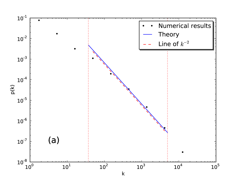
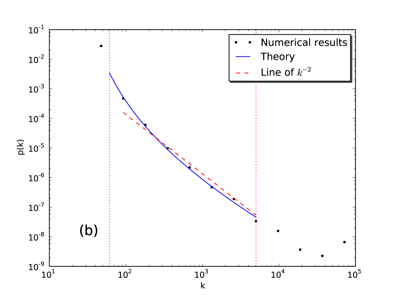
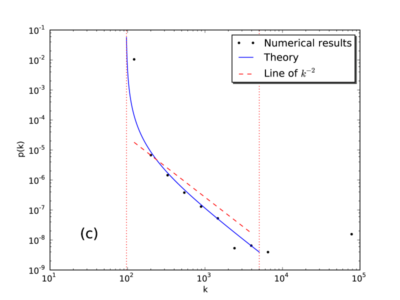
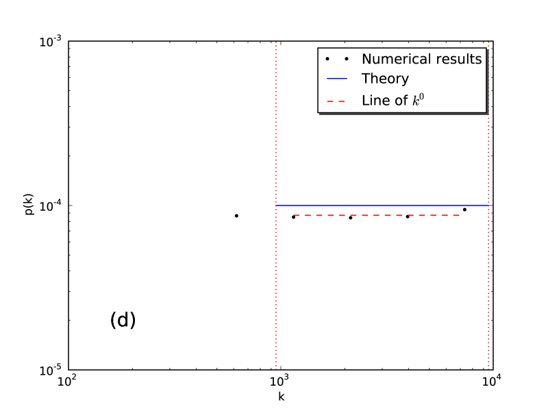
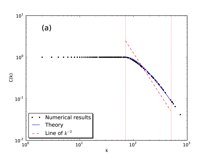
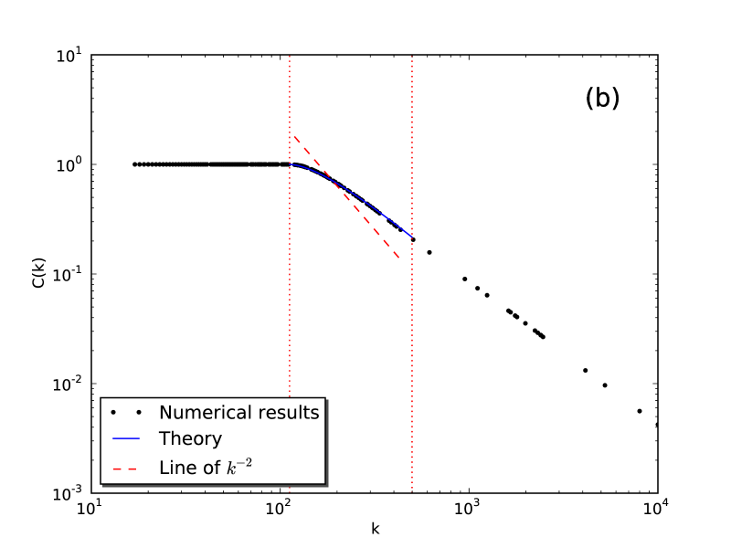
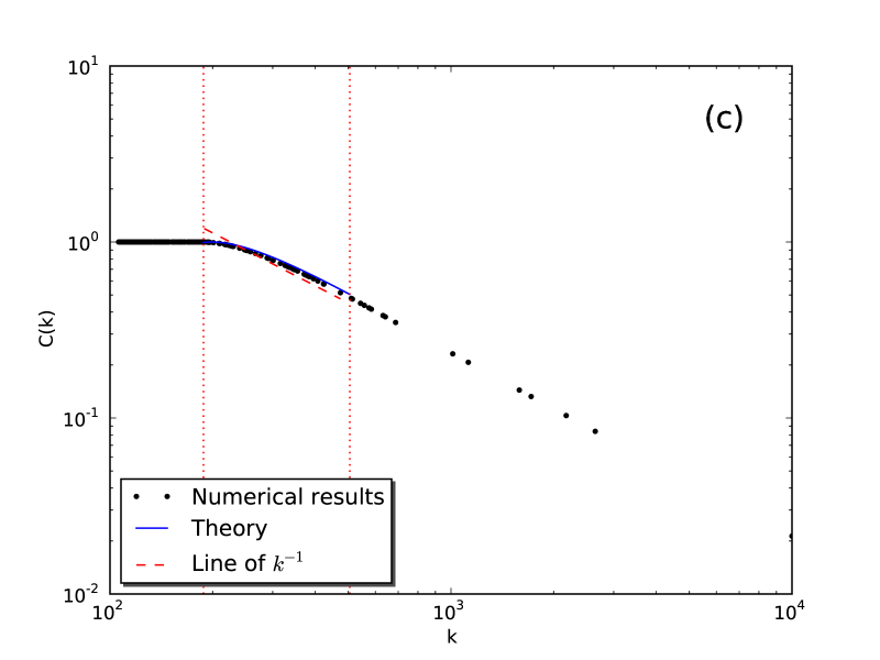
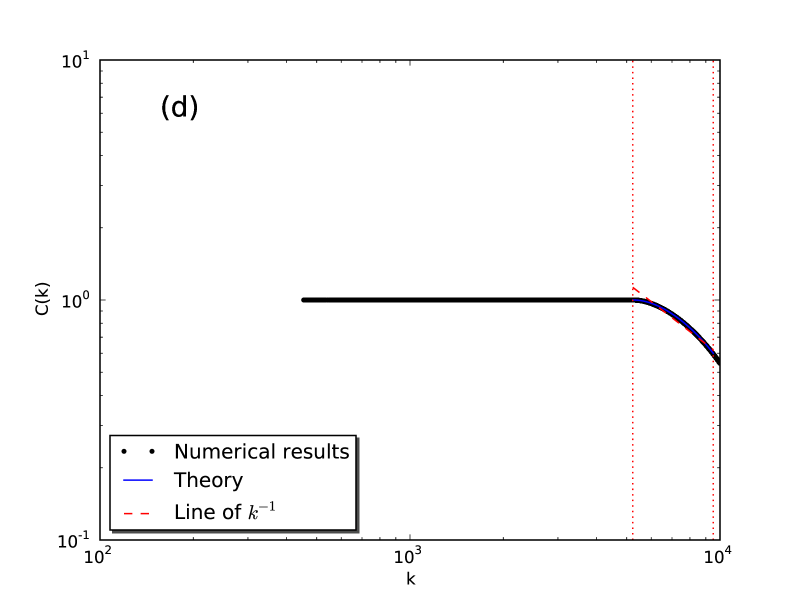
This section presents numerical results for the distributions of degrees and clustering coefficients to compare them with the theoretical results obtained in the previous section. To observe power laws, we must select the values of parameters $n$, $\theta$, and $u$ optimally with the next two items in mind. First, $\theta$ and $u$ are satisfied by the implicit condition, $\theta\geq 2u$, that prevents the applicable ranges in Eqs. (19) and  (28) from diminishing. Second, as the ranges increase as $n$ and $\theta-u$ increase, we need to give them as numerically large values as possible to identify the theoretical curves in Eqs. (14), (15), (4.2), and (24) clearly in the corresponding ranges. We determine the three parameters $n$, $\theta$, and $u$ using the following procedures. From the shape of the weight distribution function, appropriate $u$ and $\tilde{\sigma}$ are calculated using the fExtremes package [9] in R language [10]. When the value of $u$ is fixed, we give a large $\theta$ while retaining the condition $\theta\geq 2u$ and gradually increase $n$ until the universal power laws can be observed widely as well. Typical results where the weights are given by the normal and the lognormal distributions ($\xi=0$), the standard Fréchet distribution ($\xi>0$), and the uniform distribution ($\xi<0$) are given in Figs. 1 and  2. As can be seen from these figures, the theoretically predicted curves nicely fit the numerical results, meaning Eqs. (14),  (15),  (4.2), and  (24) are all accurate. Each line of power law $k^{-s}$ with $s=0$, $1$, and $2$ in the figure indicates the universal power law in Eqs. (16),  (17),  (25), and  (26). These lines are also extremely consistent with the numerical results. The plots of the numerical results around the lower bounds of the ranges appear to deviate from being linear, i.e., the power laws, because the original formulas for the degree distribution in Eq. (14) and the clustering coefficient in Eq. (4.2) are only valid in large-degree regions. Therefore, all the deviations result from small-degree effects.

Consequently, we evaluated the theoretical predictions in Sec. 4 and found they were in good agreement with the results obtained from numerical experiments in both the distributions of degrees and clustering coefficients.

6 Summary and Discussion

We analyzed the threshold network model based on extreme value theory. Where the number of nodes, $n$, and threshold $\theta$ were sufficiently large, the weight distribution function, $F(w)$, could be assumed to belong to a family of the generic weight function in Eq. (9) for $x>u$ as long as the limit distribution of maximum values for $F(w)$ converged to the distribution of GEVs in Eq. (7). As previously mentioned, many important weight functions are classified into this family; therefore, we could comprehensively treat the model with various weight functions. We then calculated the exact forms of the distributions of degrees and clustering coefficients by applying the generic weight function in Eq. (9). As a result, we found theoretical evidence for the universal power laws in Eqs. (19) and  (28), which was extremely consistent with the results obtained by Masuda et al. [4]. We also demonstrated that even though the theoretical prediction assumed a sufficiently large number of nodes, $n$, threshold value, $\theta$, and degree, $k$, the theoretical results could be reproduced through numerical experiments. This fact could explain that real complex networks with a large number of nodes and a high threshold (if they exist) could universally appear with scale-free properties.

We conclude by referring to recent mathematical studies on threshold network models [11, 12, 13]. We think that our investigation was important as a prototype to apply extreme value theory to various other models of complex networks. In future work, it would be interesting to reformulate our method mathematically to find the possibilities of extending its range of applications.

References

- [1] D. J. Watts and S. H. Strogatz, Nature 393, 440 (1998).
- [2] A. -L. Barabási and R. Albert, Science 286, 509 (1999).
- [3] G. Caldarelli, A. Capocci, P. De Los Rios, and M. A. Muñoz, Phys. Rev. Lett. 89, 258702 (2002).
- [4] N. Masuda, H. Miwa, and N. Konno, Phys. Rev. E 70, 036124 (2004).
- [5] N. Masuda, H. Miwa, and N. Konno, Phys. Rev. E 71, 036108 (2005).
- [6] P. Embrechts, C. Klüppelberg, and T. Mikosch, Modelling Extremal Events for Insurance and Finance, (Springer, Berlin, 1997).
- [7] S. Coles, An Introduction to Statistical Modeling of Extreme Values, (Springer, London, 2001).
- [8] L. de Haan and A. Ferreira, Extreme Value Theory: An Introduction, (Springer, New York, 2006).
- [9] D. Wuertz, and many others, fExtremes: Rmetrics - Extreme Financial Market Data. R package version 260.73. (2007). See the SOURCE file at http://www.rmetrics.org.
- [10] R Development Core Team, R: A language and environment for statistical computing. R Foundation for Statistical Computing, Vienna, Austria (2008). ISBN 3-900051-07-0. URL http://www.R-project.org.
- [11] N. Konno, N. Masuda, R. Roy, and A. Sarkar, Journal of Physics A: Mathematical and General, 38 6277 (2005).
- [12] Y. Ide, N. Konno, and N. Masuda, RIMS Kokyuroku, No.1551, Theory of Biomathematics and its Applications III, 81 (2007).
- [13] Y. Ide, N. Konno, and N. Masuda, Statistical Properties of a Generalized Threshold Network Model, Methodology and Computing in Applied Probability (Springer, Netherlands, 2009).